Testing for the presence of measurement error in Stata

Abstract

In this article, we describe how to test for the presence of measurement error in explanatory variables. First, we discuss the test of such hypotheses in parametric models such as linear regressions and then introduce a new command, dgmtest, for a nonparametric test proposed in Wilhelm (2018, Working Paper CWP45/18, Centre for Microdata Methods and Practice, Institute for Fiscal Studies). To illustrate the new command, we provide Monte Carlo simulations and an empirical application to testing for measurement error in administrative earnings data.

Keywords

st0600 dgmtest nonparametric test measurement error measurement error bias

1 Introduction

In this article, we describe how to test for the presence of measurement error in explanatory variables. Specifically, consider an outcome Y (for example, earnings) that depends on an explanatory variable X ^∗ (for example, schooling). We do not observe X ^∗ directly, but only two variables, X and Z, that are related to X ^∗. We suspect X is an error-contaminated measurement of X ^∗ (for example, schooling as reported in a survey) and Z is a variable related to X ^∗, perhaps an instrument (for example, distance to college) or a repeated measurement (for example, schooling as reported in another survey). The hypothesis of no measurement error in X is

H_{0} : P (X = X^{*}) = 1

In the schooling example, testing H ₀ could be useful as a first-step model specification test to tell the researcher whether measurement error is an important feature of the data that should be modeled. However, testing H ₀ may be of direct economic interest because, for example, the null of no measurement error can often be shown to be implied by the absence of frictions in a structural economic model (for example, Chetty [2012]; Wilhelm [2018]). Therefore, a test of H ₀ can be interpreted as a test of the absence of such frictions.

In a finite sample, we may not be able to detect measurement error even though X is in fact mismeasured, because measurement errors might be small relative to the overall sampling noise. In this sense, we can interpret the test of H ₀ as finding out whether measurement error is severe enough for the data to tell the difference between models with and without measurement error.

In this article, we describe how to test for the presence of measurement error without imposing any parametric restrictions and, in fact, without requiring the model to be identified. Both of these aspects are important for empirical practice. First, when one tests for measurement error, it is important to allow for nonlinearities in the relationship of Y and X ^∗ because measurement error in X can make the relationship appear nonlinear when it is not and make it appear linear when it is not (Chesher 1991). Therefore, to disentangle measurement error from nonlinearities requires a procedure that can allow for nonlinearities. Second, nonparametric measurement error models are identified only under fairly strong conditions, and their estimation involves complicated procedures such as Fourier transforms and operator inversions (Schennach 2013, 2016; Hu 2017). However, Wilhelm (2018) shows that testing for the presence of measurement error does not require identification of the model and is thus possible without such strong assumptions. In particular, the test can detect many nonclassical measurement error models, that is, models in which the measurement error depends on the true latent variable. Another by-product of avoiding identification of the model is that complicated estimation techniques are not necessary. In fact, the test we describe employs only standard nonparametric regression techniques.

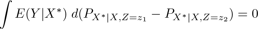
The null hypothesis depends on the latent variable X ^∗ and thus cannot directly be tested. In section 2, therefore, we first describe how to convert the null hypothesis into a testable restriction in terms of the observable variables Y, X, Z in a simple example, a linear regression model. In this model, H ₀ can easily be tested using existing Stata commands following Hausman (1978). Section 3 then describes the extension of such ideas to the nonparametric framework as recently proposed by Wilhelm (2018). We also introduce a new command, dgmtest, that implements a test of H ₀ without imposing any parametric restrictions. Section 4 reports the results of Monte Carlo simulations for dgmtest, and section 5 concludes with an empirical example in which we show how to test for measurement error in administrative earnings data.

Related literature

Mahajan (2006) proposes a test for the presence of measurement error when the explanatory variable X ^∗ and the observed measure X are binary. There are some existing tests for the presence of measurement error in parametric models that require identification and consistent estimators of the model: Hausman (1978); Chesher (1990); Chesher, Dumangane, and Smith (2002); Hahn and Hausman (2002); and Hu (2008). Related to Hausman (1978), in empirical work it is common to estimate linear regressions by ordinary least squares (OLS) and instrumental variables (IV) and then attribute a difference in the two estimates to the presence of measurement error, treating the IV estimate as the consistent and unbiased one. Of course, this strategy is valid only if the true relationship of interest is actually linear, the measurement error is classical, and the model is identified. None of these assumptions is required in the nonparametric approach described in this article.

In principle, one could imagine constructing a test for the presence of measurement error by comparing an estimator of the model that accounts for the possibility of measurement error with one that ignores it, similar in spirit to the work by Durbin (1954), Wu (1973), and Hausman (1978). If the difference between the two is statistically significant, then one could conclude that this is evidence for the presence of measurement error. However, this strategy would require identification and consistent estimation of the measurement error model, which leads to overly strong assumptions, the necessity of solving ill-posed inverse problems in the continuous variable case, and potentially highly variable estimators. These difficulties can all be avoided by the nonparametric approach described in this article.

2 Linear regression model

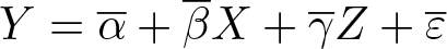
Consider the linear regression model for an outcome Y and an explanatory variable X ^∗, assuming for simplicity that there are no further regressors (the extension to the presence of additional controls is straightforward and discussed below),

Y = α + β X^{*} + ε E (ε X^{*}) = 0

Instead of X ^∗, we observe a measurement X of X ^∗ and IV Z, which depends on X ^∗ [that is, E(X ^∗ Z) ≠ 0], but is excluded from the outcome equation [that is, E(εZ) = 0]. Testing for the presence of measurement error in this context is straightforward (Hausman 1978). Under the null of no measurement error, OLS consistently estimates β, but under the alternative of some measurement error, it is inconsistent. The IV estimator, however, is consistent under both the null and the alternative. Therefore, one can simply compute both estimators and compare them. If their difference is statistically significant, that indicates the presence of measurement error.

To better understand the connection to the nonparametric test described in the next section, note that the test based on the difference of OLS and IV estimators is equivalent to testing significance in an expanded regression. To see this, suppose there is no measurement error in X, then

Y = α + β X + ε E (ε X) = 0

Therefore, when we regress Y onto both X and Z, the exclusion of the IV implies that the coefficient of Z must be zero;¹ that is, we test the hypothesis of no measurement error by instead testing

\bar{γ} = 0

in the regression

Y = \bar{α} + \bar{β} X + \bar{γ} Z + \bar{ε}

In conclusion, we have shown that the null of no measurement error, (1), implies (3) in the linear regression model. The only assumption for this to be true is that (2) holds and that the IV is excluded from the outcome equation; that is, E(εZ) = 0. Therefore, a rejection of the restriction (3) implies a rejection of the hypothesis of no measurement error, (1).

However, without further assumptions, failing to reject (3) does not necessarily imply failing to reject the null of no measurement error, (1). Suppose X = X ^∗ + η_X so that η_X represents the measurement error in X. If the measurement error in X is assumed to be classical [that is, it is uncorrelated with the latent regressor, E(X ^∗ η_X ) = 0] and uncorrelated with the regression error, E(εη_X ) = 0, and if some further regularity conditions hold, then it is easy to see that the null hypothesis H ₀ not only implies but also is in fact implied by (3). Therefore, failing to reject (3) may be interpreted as failing to reject H ₀, and rejecting (3) may be interpreted as rejecting H ₀.

Consider the following simulated example that illustrates the finite sample performance of the test by Hausman (1978). First, we simulate data without measurement error in the regressor (X = X ^∗),

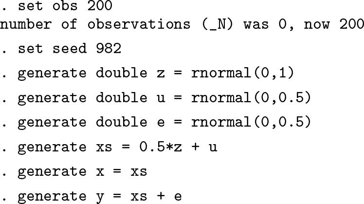
Then, we regress Y on X and Z (and a constant),

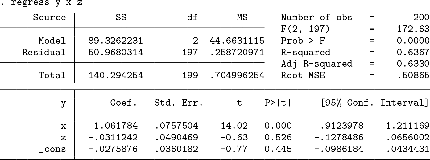
to find that Z is not significant at any reasonable confidence level (p-value is 0.526). Therefore, we fail to reject the null of no measurement error as expected. Now, we generate a measurement error contaminated regressor (X ≠ X ^∗),

. generate double eta = rnormal(0,0.5)

. drop x

. generate x = xs + eta

Again, we regress Y on X and Z (and a constant),

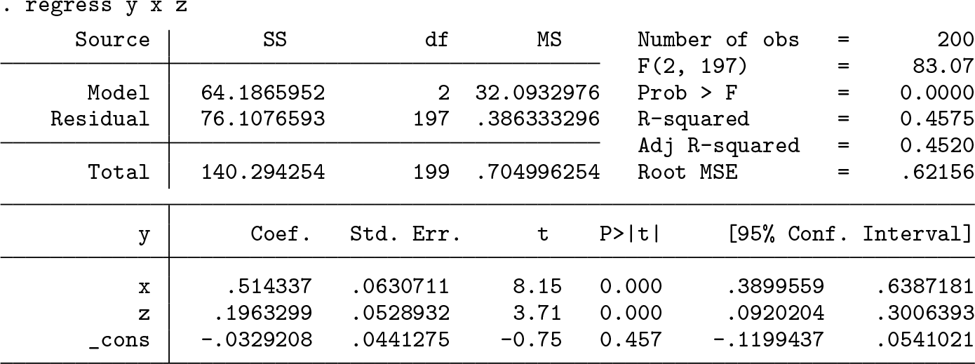
to find that now Z is significant at every reasonable confidence level (p-value is 0.000). Therefore, we strongly reject the null of no measurement error.

In the presence of additional, correctly measured controls in the regression model, we would proceed exactly as above except that we would include the additional controls in the regression command.

3 Nonparametric model—The new dgmtest command

While the approach to testing H ₀ in the previous section is straightforward and intuitive, its validity relies on strong assumptions: linearity in the outcome equation and classical measurement error in X. Because nonlinearities in the regression equation and measurement error in X may manifest themselves similarly (Chesher 1991), it is important to allow for nonlinearities in the relationship between Y and X ^∗ when testing for measurement error. In addition, a large literature has documented that measurement error in economic data is rarely classical (see the survey by Bound, Brown, and Mathiowetz [2001], for example). In this section, we describe how to test H ₀ in nonlinear models with nonclassical measurement error.

Suppose the variable Z is related to X ^∗, but the measurement X is excluded from the outcome model in the sense that

E (Y | X^{*}, X, Z) = E (Y | X^{*}) a . s .

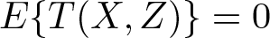
That is, they can affect outcomes only through the true explanatory variable X ^∗. Then, it is easy to see that, under H ₀, Z must be excluded from the outcome equation conditional on the observed X,

E (Y | X, Z) = E (Y | X) a . s .

Unlike H ₀, this is a restriction that depends only on observables and can directly be tested without making any parametric assumptions about how the conditional mean of Y depends on X ^∗. The test by Delgado and González Manteiga (2001) introduced

in the next subsection and implemented in the new command, dgmtest, for instance, directly tests the restriction (5). Because of the above argument, it can be interpreted as a test of the original null of interest, the null of no measurement error in (1).

The exclusion restriction (4) is standard in the literature on identification and estimation of measurement error models (Carroll et al. 2006; Chen, Hong, and Nekipelov 2011; Schennach 2013, 2016; Hu 2017) and has already been justified in many empirical applications. Because the assumption is central to the validity of the test for measurement error, we now provide a few examples.

Consider a generic production problem in which Y is an output that is produced from a vector of inputs X ^∗. The inputs are measured by the vectors X and Z alternatively. In this context, the exclusion restriction is often a natural assumption because it requires the “true” inputs X ^∗ to be the factors that matter for production, not the measurements (X, Z). Therefore, conditional on knowing X ^∗, the measurements X and Z should not provide any additional information about the output Y . Cunha, Heckman, and Schennach (2010); Heckman, Pinto, and Savelyev (2013); Attanasio et al. (2015); and Attanasio, Meghir, and Nix (2017) are examples of empirical articles in the skillformation literature that have justified the exclusion restriction in this fashion. The same argument applies to many other production problems in which inputs are difficult to measure (for example, Olley and Pakes [1996]).

In the empirical part of Wilhelm (2018) and in section 5 below, Y , X, and Z are three measurements of earnings, but Y and (X, Z) come from two different data sources, one from a survey and the other from an administrative dataset. We then argue the exclusion restriction holds because the error in Z has a different origin from the error in Y , at least conditional on X ^∗.

There are many other empirical applications that impose the exclusion restriction (4): For instance, Altonji (1986) studies labor supply; Kane and Rouse (1995) and Kane, Rouse, and Staiger (1999) study the returns to education; Card (1996) studies the effect of unions on the wage structure; Hu et al. (2013) study auctions with unobserved heterogeneity; Feng and Hu (2013) study unemployment dynamics; and Arellano, Blundell, and Bonhomme (2017) study earnings dynamics.

Wilhelm (2018) actually shows that, under additional assumptions, H ₀ not only implies but also is implied by the observable restriction (5). Therefore, failing to reject (5) may be interpreted as failing to reject H ₀, and rejecting (5) may be interpreted as rejecting H ₀.

The main assumptions required for this equivalence result are first, the exclusion restriction (4); second, a relevance condition that ensures Z is sufficiently strongly related to X ^∗; and third, monotonicity of the conditional mean function $x^{*} \mapsto E (Y | X^{*} = x^{*})$ .

To satisfy the relevance condition, we need to find two values of Z, say, z ₁ , z ₂, such that the probability mass functions of $X^{*} | Z = z_{1}$ and $X^{*} | Z = z_{2}$ do not cross more than once. This assumption is testable under the additional assumption that X and X ^∗ are sufficiently strongly monotonically related because, in that case, we must have that the probability mass functions of $X | Z = z_{1}$ and $X | Z = z_{2}$ do not cross more than once (see appendix A.3 in Wilhelm [2018]). Finally, monotonicity of the relationship between the outcome and the explanatory variable is a weak assumption that is often directly implied by economic theory, for example, when the conditional mean $E (Y | X^{*} = x^{*})$ is a production, cost, or utility function. Examples can be found in Matzkin (1994); Olley and Pakes (1996); Cunha, Heckman, and Schennach (2010); Blundell, Horowitz, and Parey (2012, 2017); Kasy (2014); Wilhelm (2015); Hoderlein et al. (2015); and Chetverikov and Wilhelm (2017), among many others.

We now heuristically explain why the exclusion restriction, the relevance condition, and the monotonicity condition together guarantee equivalence of H ₀ and (5). We have already argued why H ₀ implies (5) under the exclusion restriction, so we need to show only that the reverse holds as well.

Consider the special case when X ^∗ and X are continuously distributed and X ^∗, X, and Z are scalars. Suppose the observable implication (5) holds. Then, for any two values z ₁ , z ₂, we have $E (Y | X, Z = z_{1}) = E (Y | X, Z = z_{2})$ . Then, by the exclusion restriction,

\int E (Y | X^{*}) d (P_{X^{*}} {_{| X, Z}}_{= z_{1}} - P_{X^{*}}_{| X, Z = z_{2}}) = 0

if E(Y |X ^∗ = ·) is differentiable, then integration by parts yields

\int P {X^{*} | X = x, Z = z_{1} (x *) - P X^{*} | X = x, Z = z_{2} (x^{*})} \frac{\partial E (Y | X^{*} = x^{*})}{\partial x^{*}} d x^{*} = 0

We want to show that this equation implies the null hypothesis H ₀. On the contrary, assume that this is not the case. To generate a contradiction, we want to ensure that (6) does not hold under the alternative H ₁. This is the case, for example, when E(Y |X ^∗ = ·) is monotone (and not constant) and $P_{X^{*}} {_{| X}}_{= x, Z = z_{2}}$ first-order stochastically dominates $P_{X} *_{| X}_{= x, Z = z_{1}}$ (and they are not equal) under H ₁. The relevance condition of Wilhelm (2018) ensures that this first-order stochastic dominance holds. The monotonicity assumption, on the other hand, implies that the derivative of the conditional expectation does not change sign (and is nonzero somewhere), and the dominance condition implies that the difference of the conditional distributions is nonnegative (and positive somewhere). In conclusion, the integral in (6) is nonzero under H ₁, yielding the desired contradiction, so the null of no measurement error must hold. For more details on the exact assumptions and arguments, see Wilhelm (2018).

In some applications, Z may be excluded from the outcome equation only after conditioning on some additional, correctly measured controls W; that is, the exclusion restriction (4) is replaced by

E (Y | X^{*}, W, X, Z) = E (Y | X^{*}, W) a . s .

This additional conditioning on W is necessary, for example, in cases in which W determines both Y and (X, Z). Under (7), the null hypothesis H ₀ then implies

E (Y | X, W, Z) = E (Y | X, W) a . s .

The null hypothesis is, in fact, equivalent to (8) under conditions like those required for the equivalence of H ₀ and (5). In the implementation of the test, we allow for two types of additional controls, say, W = (W ₁, W ₂), where the vector W ₁ is included in the conditional mean in a nonseparable fashion and the vector W ₂ is additively separable and linear,

E (Y | X, W) = g (X, W_{1}) + π^{'} W_{2}

for some function g and some vector of coefficients π .

There exist many nonparametric tests of the conditional mean independence in (5) and (8), for example, Gozalo (1993); Fan and Li (1996); Delgado and González Manteiga (2001); Mahajan (2006); and Huang, Sun, and White (2016). Therefore, any of those could be used for nonparametrically testing for the presence of measurement error. In the presence of several additional covariates W, however, the curse of dimensionality may cause fully nonparametric tests to be infeasible. Therefore, we recommend the semiparametric, partially linear model in (9) as a more practical approach in such cases.

In the following subsections, we introduce a new command, dgmtest, that implements the test by Delgado and González Manteiga (2001). This test has some desirable properties such as relatively simple implementation and its ability to detect alternatives at the $\sqrt{n}$ -rate.

3.1 The test by Delgado and González Manteiga (2001)

We briefly describe the approach by Delgado and González Manteiga (2001) for testing the conditional mean independence (5). There are many other reasons why one might want to test such a restriction, and the test for the presence of measurement error as described in this article is only one of these. To simplify the description, we focus on the case in which there are no additional controls W .

The authors rewrite the null hypothesis of conditional mean independence, (5), as

\begin{array}{l} E {T (X, Z)} = 0 \end{array}

where

T (x, z) : = E f_{X} (X) Y - E (Y | X) 1 {X \leq x} 1 {Z \leq z}

1{A} is equal to 1 if the event A holds, 0 otherwise, and f_X is the density of X. Given a random sample ${(Y_{i}, X_{i}, Z_{i})}_{i = 1}^{n}$ from the distribution of (Y, X, Z), consider the empirical analogue T_n (x, z) of T (x, z),

T_{n} (x, z) : = \frac{1}{2_{n}} \sum_{i} \sum_{j} \frac{1}{h} K (\frac{X_{i} - X_{j}}{h}) (Y_{i} - Y_{j}) 1 {X_{i} \leq x} 1 {Z_{i} \leq z}

where h is a bandwidth parameter and K a kernel function. Delgado and González Manteiga (2001) propose two test statistics: the Cramér–von Mises statistic $T_{n} : = n \sum_{i = 1}^{n} T_{n} {(X_{i}, Z_{i})}^{2}$ and the Kolmogorov–Smirnov statistic $T_{n} : = s u p_{x, z} | \sqrt{n} T_{n} (x, z) |$ . Critical values of the test are computed using the bootstrap procedure described in Delgado and González Manteiga (2001).

Testing the version with additional controls, (8), is a simple extension of the above test. In the presence of additively separable controls W ₂, we perform the test in two steps. First, we compute an estimator $\hat{π}$ of π as in Robinson (1988). Then, we apply Delgado and González Manteiga’s (2001) test as described above, replacing Y_i by $Y_{i} - \hat{π}' W_{2 i}$ .

3.2 Syntax

The dgmtest command implements the test by Delgado and González Manteiga (2001). The syntax of the command is

dgmtest depvar expvar [ if ] [ in ] [ , qz( # ) qw2( # ) teststat( string ) kernel( string ) bootdist( string ) bw( # ) bootnum( # ) ngrid( # ) qgrid( # )]

The two required arguments of the command are depvar (the outcome variable Y ) and expvar (a list of variables containing all elements of X, W ₁, W ₂, and Z). Therefore, expvar should consist of at least two variables, in which case the first is taken to be X and the second to be Z. If there are more than two variables, then the options qz() and qw2() determine which variables in the list are X, W ₁, W ₂, and Z. For instance, if expvar contains 6 variables, qz() equals the default value of 1, and qw2() is equal to 2, then the first 3 variables in the list are interpreted as (X, W ₁) (which one is X and which one is W ₁ does not matter because the test treats both types of variables exactly the same), the fourth and fifth variables are interpreted as W ₂, and the sixth variable as Z.

3.3 Options

qz( # ) is the dimension of Z. The default is qz(1).

qw2( # ) is the dimension of W ₂. The default is qw2(0), which means there are no additional controls W ₂.

teststat( string ) is the type of test statistic to be used: CvM and KS represent the Cramér–von Mises and Kolmogorov–Smirnov statistics, respectively. The default is teststat(CvM).

kernel( string ) is the kernel function. The default kernel is the Epanechnikov kernel (epanechnikov). Alternatively, we can choose one among two other Epanechnikov kernels order of 2 and 4 with the support [−1, 1] (epan2 and epan4), biweight kernel (biweight), Gaussian kernel (normal), rectangle kernel (rectangle), and triangular kernel (triangular).

bootdist( string ) is the distribution of the bootstrap multiplier variable. Following Delgado and González Manteiga (2001), it should have a zero mean and unit variance. The default is bootdist(mammen) in Härdle and Mammen (1993), which is the two-point distribution attaching masses $(\sqrt{5} + 1) / 2 \sqrt{5}$ and $(\sqrt{5} - 1) / 2 \sqrt{5}$ to the points $- (\sqrt{5} - 1) / 2$ and $\sqrt{5} + 1 / 2$ , respectively. Alternatively, we can choose the Rademacher distribution (rademacher) or the continuous uniform distribution on $- \sqrt{3}, \sqrt{3}$ (uniform).

bw( # ) is the bandwidth h, taken to be the same for every component of (X, W ₁). The default is n ^−1/3q, which is a rule of thumb in Delgado and González Manteiga (2001), where n is the sample size and q is the dimension of (X, W ₁).

bootnum( # )is the number of bootstrap samples for the computation of the test’s critical value. The default is bootnum(500).

ngrid( # ) is the number of equally spaced grid points used to compute the supremum of the Kolmogorov–Smirnov statistic if that statistic is chosen via the option teststat(). The default is ngrid(0), which means that the sample serves as the grid. ngrid(0) is required for calculating the exact Kolmogorov–Smirnov statistic, but it is a burden when we perform a simulation with a large sample, so one might want to choose a positive number smaller than the sample size in that case. The user need not specify this if teststat(CvM) is used.

qgrid( # ) is a quantile probability between 0 and 1 to set the minimum and maximum values of the grid points in the previous option. If qgrid() is smaller than 0.5, the minimum value is the qgrid() quantile, and the maximum value is the 1-qgrid() quantile. The default is grid(0), so in that case, the grid ranges from the minimum to the maximum value in the sample. The user need not specify this if teststat(CvM) is used.

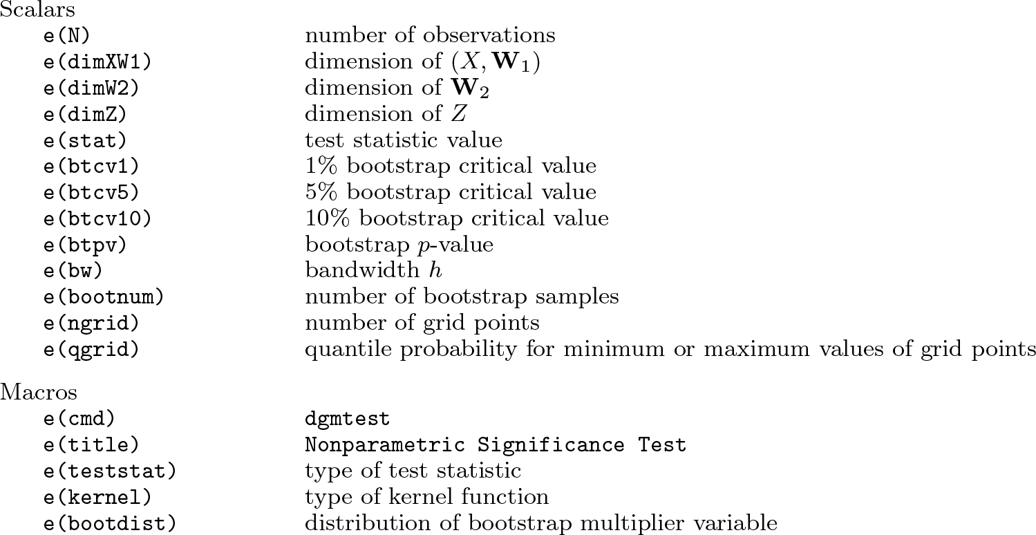
3.4 Stored results

dgmtest stores the following in e():

3.5 A simple example

Consider again the simple simulated example from section 2. First, perform the non-parametric test for measurement error on the correctly measured explanatory variable, using the default settings of the dgmtest command:

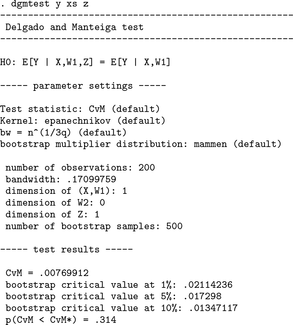
The p-value of the Cramér–von Mises version of the test is 0.314, which means we fail to reject the null of no measurement error at all reasonable confidence levels.

Now, we perform the test on the mismeasured explanatory variable, again using the default settings of the command:

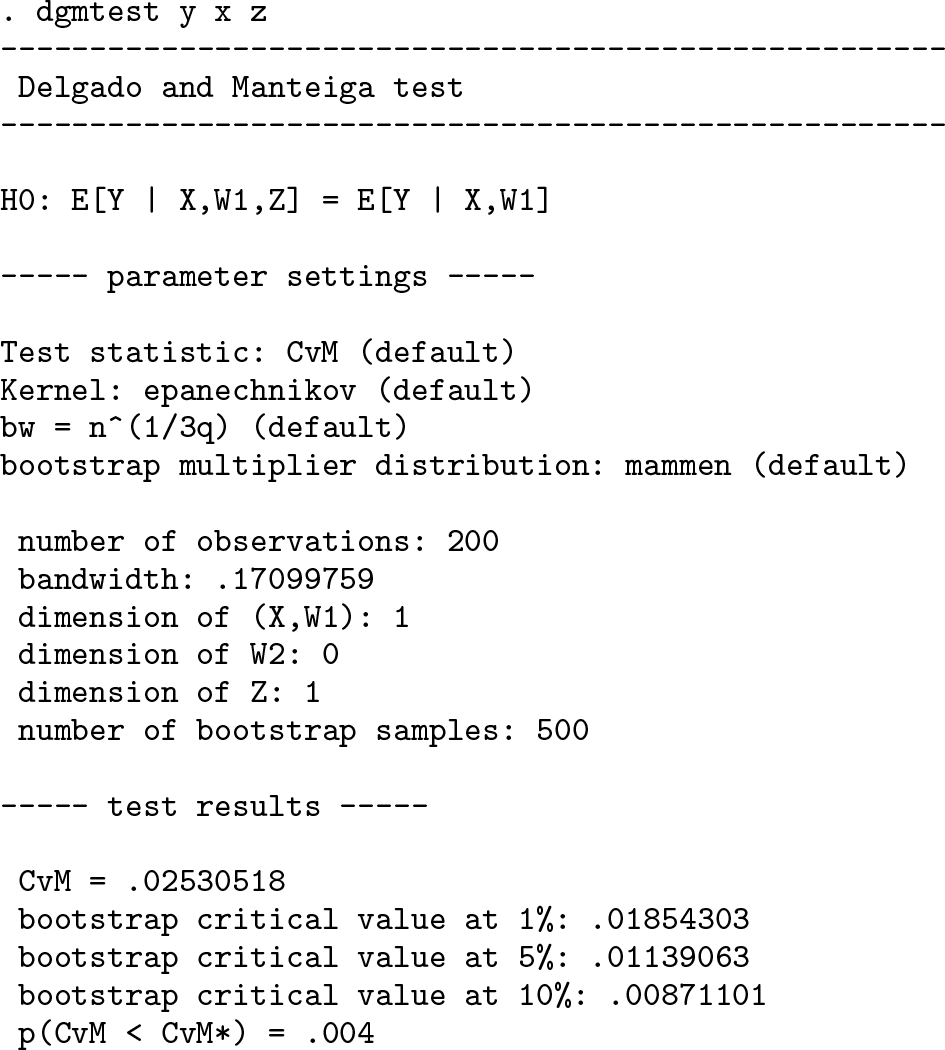
As expected, the nonparametric test detects the measurement error and strongly rejects the null of no measurement error (p-value is 0.004) at all reasonable confidence levels.

4 Monte Carlo simulation

In this section, we present a small simulation study investigating the finite sample performance of the measurement error test.

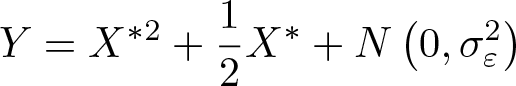
We consider the outcome equation

Y = X^{* 2} + \frac{1}{2} X^{*} + N (0, σ_{ε}^{2})

with different models for the measurement system:

Model I : $X = X^{*} + D \times N (0, σ_{ME}^{2})$ , $Z = X^{*} + N 0, {0.3}^{2}$

Model II : $X = X^{*} + D \times N (0, σ_{ME}^{2}) e^{- | X^{*} - 0.5 |}$ , $Z = X^{*} + N 0, {0.3}^{2}$

Model III : $X = X^{*} + D \times N (0, σ_{ME}^{2}) e^{- | X^{*} - 0.5 |}$ , $Z = X^{*} + N (0, {0.3}^{2}) e^{- | X^{*} - 0.5 |}$

Model IV : $X = X^{*} + D \times N (0, σ_{ME}^{2})$ , $Z = - (X^{*} - 1) 2 + N 0, {0.2}^{2}$

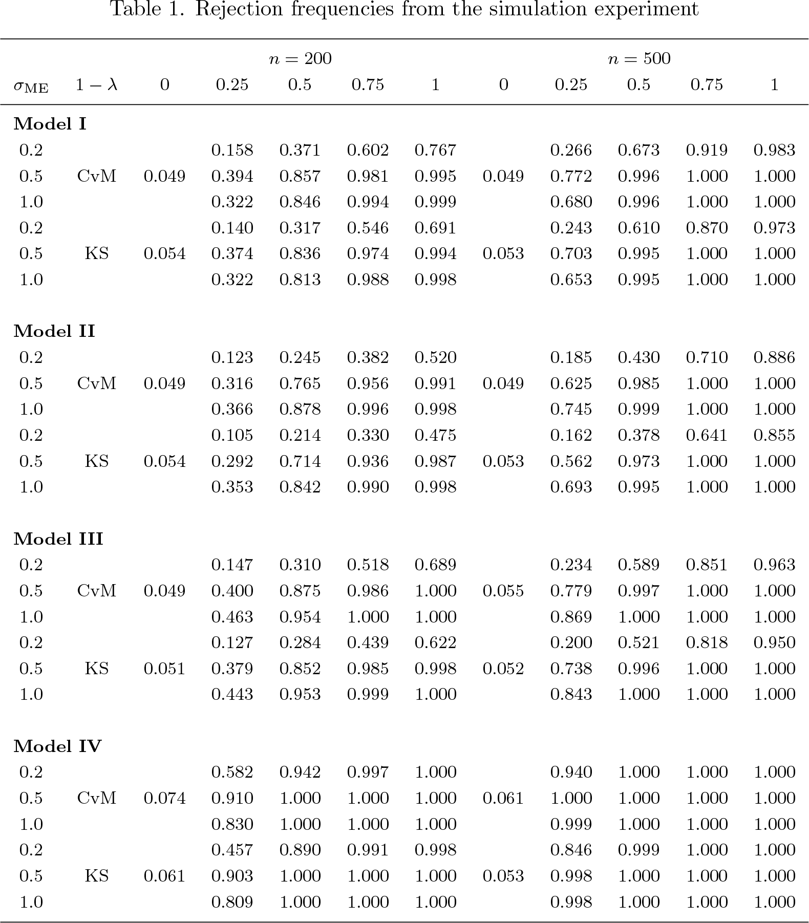
The value for σ_ε is 0.5 for models I, II, and III and 0.2 for model IV. In all four models, X ^∗ ∼ U [0, 1], and the random variable D is Bernoulli(1 − λ), where 1 − λ is the probability of measurement error (ME) in X occurring. 1 − λ = 0 means there is no measurement error in X, which represents the null hypothesis. To generate alternatives, we increase 1−λ on a grid up to 1. We vary the standard deviation of the measurement error in X, σ _ME, in {0.2, 0.5, 1}. Therefore, alternatives get closer to the null as we decrease 1 − λ or σ _ME, or both. We vary the sample size n ∊ {200, 500}, but all models are simulated on 1,000 Monte Carlo samples (we set the seed at 1234). Following Delgado and González Manteiga (2001), we use the bandwidth rule-of-thumb value n ^−1/3. Simulation results for different choices of bandwidths, which are not presented here, are similar.

The Cramér–von Mises statistics are generated by

. dgmtest Y X Z, kernel(epan2) bootnum(100)

The Kolmogorov–Smirnov test statistics with 10 grid points are generated by

. dgmtest Y X Z, teststat(KS) kernel(epan2) bootnum(100) ngrid(10) qgrid(0.05)

Table 1 shows the rejection frequencies of the test. Overall, the test controls size well and possesses power against all alternatives. These findings are consistent with the Monte Carlo simulation results in Wilhelm (2018).

Table 1.

Rejection frequencies from the simulation experiment

n = 200							n = 500
_ME	1 − λ	0	0.25	0.5	0.75	1	0	0.25	0.5	0.75	1
Model I
0.2			0.158	0.371	0.602	0.767		0.266	0.673	0.919	0.983
0.5	CvM	0.049	0.394	0.857	0.981	0.995	0.049	0.772	0.996	1.000	1.000
1.0			0.322	0.846	0.994	0.999		0.680	0.996	1.000	1.000
0.2			0.140	0.317	0.546	0.691		0.243	0.610	0.870	0.973
0.5	KS	0.054	0.374	0.836	0.974	0.994	0.053	0.703	0.995	1.000	1.000
1.0			0.322	0.813	0.988	0.998		0.653	0.995	1.000	1.000
Model II
0.2			0.123	0.245	0.382	0.520		0.185	0.430	0.710	0.886
0.5	CvM	0.049	0.316	0.765	0.956	0.991	0.049	0.625	0.985	1.000	1.000
1.0			0.366	0.878	0.996	0.998		0.745	0.999	1.000	1.000
0.2			0.105	0.214	0.330	0.475		0.162	0.378	0.641	0.855
0.5	KS	0.054	0.292	0.714	0.936	0.987	0.053	0.562	0.973	1.000	1.000
1.0			0.353	0.842	0.990	0.998		0.693	0.995	1.000	1.000
Model III
0.2			0.147	0.310	0.518	0.689		0.234	0.589	0.851	0.963
0.5	CvM	0.049	0.400	0.875	0.986	1.000	0.055	0.779	0.997	1.000	1.000
1.0			0.463	0.954	1.000	1.000		0.869	1.000	1.000	1.000
0.2			0.127	0.284	0.439	0.622		0.200	0.521	0.818	0.950
0.5	KS	0.051	0.379	0.852	0.985	0.998	0.052	0.738	0.996	1.000	1.000
1.0			0.443	0.953	0.999	1.000		0.843	1.000	1.000	1.000
Model IV
0.2			0.582	0.942	0.997	1.000		0.940	1.000	1.000	1.000
0.5	CvM	0.074	0.910	1.000	1.000	1.000	0.061	1.000	1.000	1.000	1.000
1.0			0.830	1.000	1.000	1.000		0.999	1.000	1.000	1.000
0.2			0.457	0.890	0.991	0.998		0.846	0.999	1.000	1.000
0.5	KS	0.061	0.903	1.000	1.000	1.000	0.053	0.998	1.000	1.000	1.000
1.0			0.809	1.000	1.000	1.000		0.998	1.000	1.000	1.000

5 Example: Testing for the presence of measurement error in administrative earnings data

In this section, we test for measurement error in the U.S. Social Security Administration’s measure of earnings. While measurement error in survey responses is a widespread concern that has occupied a large literature (Bound, Brown, and Mathiowetz 2001), only recently empirical researchers have emphasized concerns about the reliability of administrative data (for example, Fitzenberger, Osikominu, and Völter [2006]; Kapteyn and Ypma [2007]; Abowd and Stinson [2007]; Groen [2012]).

The data come from the March 1978 Current Population Survey/Social Security Summary Earnings (U.S. Census Bureau 2009). The sample selection is similar to Wilhelm (2018), except that we consider only white singles between ages 25 and 60 who work full time the full year. The sample size is 2,683 individuals. The dataset contains a survey measure of earnings in 1977 (repearn77) from the Current Population Survey and two administrative measures of earnings in 1977 and in 1976 (ssearn77 and ssearn76), the earnings records of the social security administration. We denote by Y the survey measure and by X and Z the administrative measures in 1977 and 1976, respectively. A test for the presence of measurement error in X as in H ₀ is then a test of the presence of measurement error in administrative earnings in 1977.

Figure 1 shows nonparametric density estimates of survey and administrative earnings. Figure 2 plots the nonparametric density estimate of the difference between administrative and survey earnings. There is substantial probability mass within USD ±1,000, which is a large deviation relative to the maximum earnings in the sample (USD 16,500).

Figure 1.

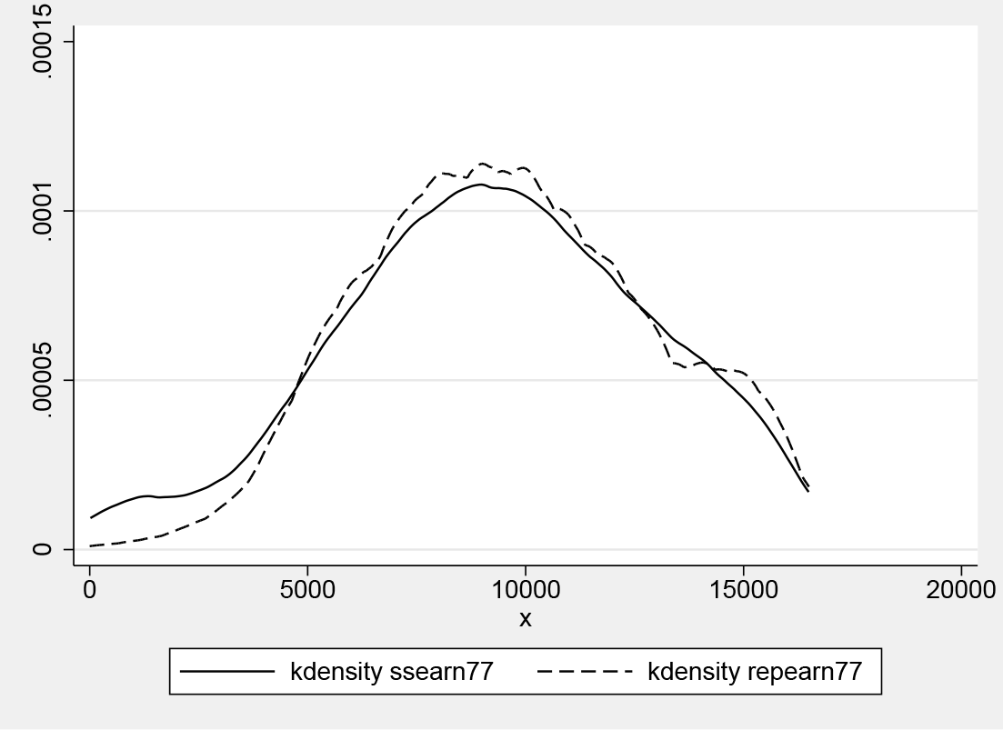
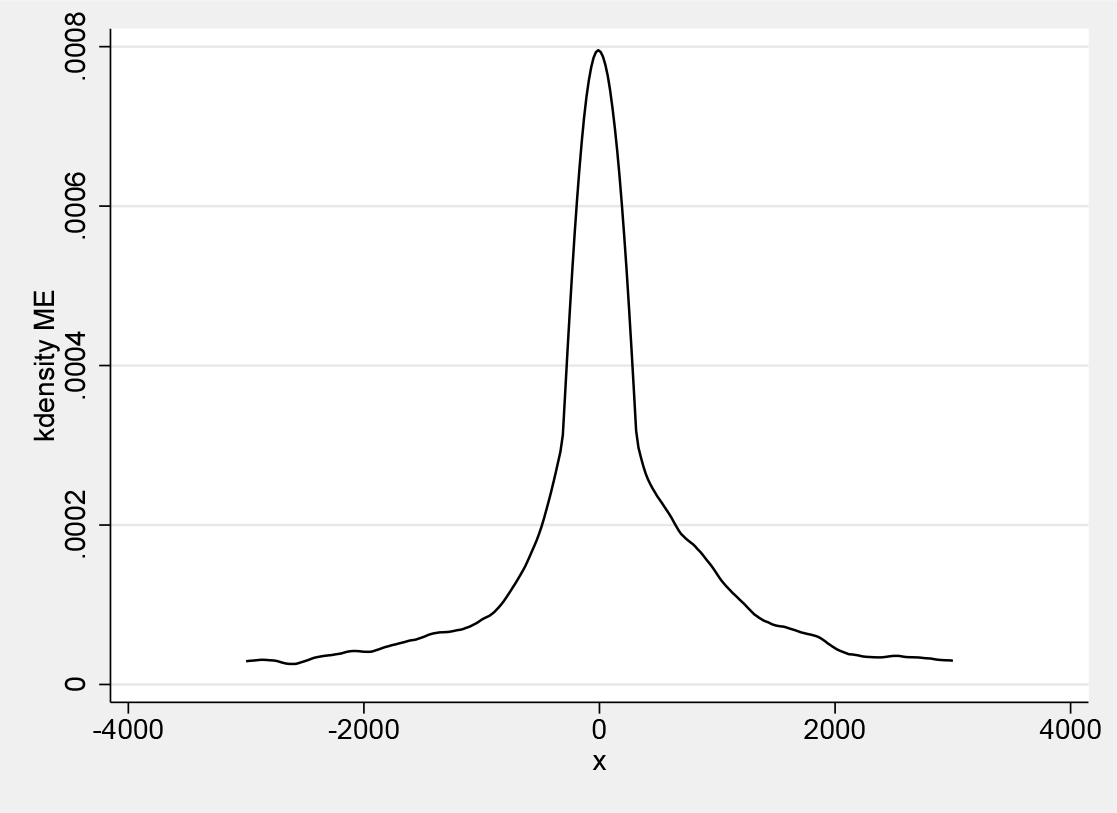
Nonparametric density estimates of administrative earnings (ssearn77) and survey earnings (repearn77) in 1977, using cross-validated bandwidths

Figure 2.

Nonparametric density estimate of the difference in administrative and survey earnings in 1977, using a cross-validated bandwidth

The exclusion restriction (4) is likely to hold in this context because the measurement errors in survey and administrative earnings come from different sources (see the more detailed discussion in Wilhelm [2018]). To assess the relevance of the second measurement Z, which here is lagged administrative earnings, we plot the density of administrative earnings in 1977 given those in 1976. Figure 3 shows this density for those individuals with lagged earnings in the 10th and 90th percentile of the 1976 earnings distribution. The graph shows that the second measurement Z, lagged administrative earnings, shifts the earnings distribution in the next period to the right as we go from the 10th to the 90th percentile. In particular, the two densities seem to cross only once, which is consistent with the relevance condition that is needed for the equivalence of H ₀ and the observable restriction (5).

Figure 3.

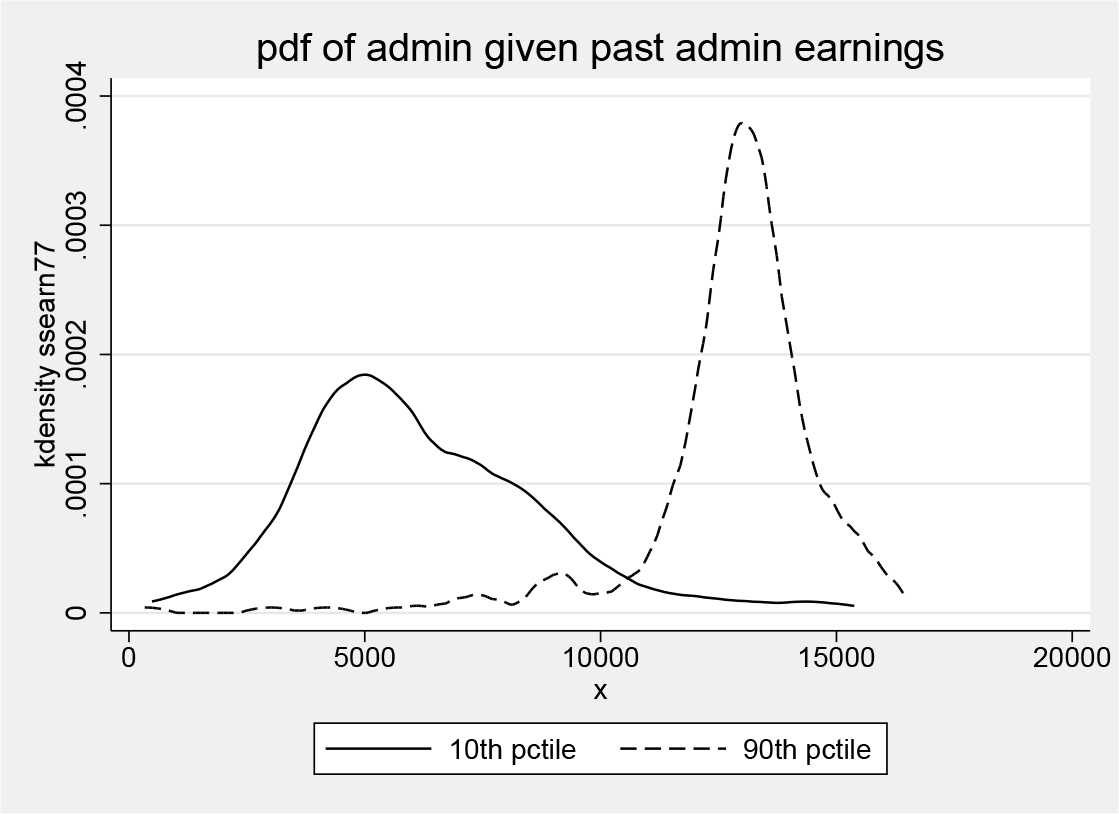
Nonparametric estimate of the conditional density of administrative earnings in 1977 given lagged administrative earnings being in the 10th or 90th percentile. Bandwidths are chosen by cross-validation.

Figure 4 shows nonparametric estimates of the conditional mean E(Y |X = x, Z = z) as a function of z for three values of x. If there was no measurement error in X, then (5) implies that this conditional mean should not vary with z. The graph suggests that there is some variation in that dimension, particularly for small and large values of earnings, but the graph does not contain any information about whether this variation is statistically significant, so we will now discuss the results of the formal test of H ₀.

Figure 4.

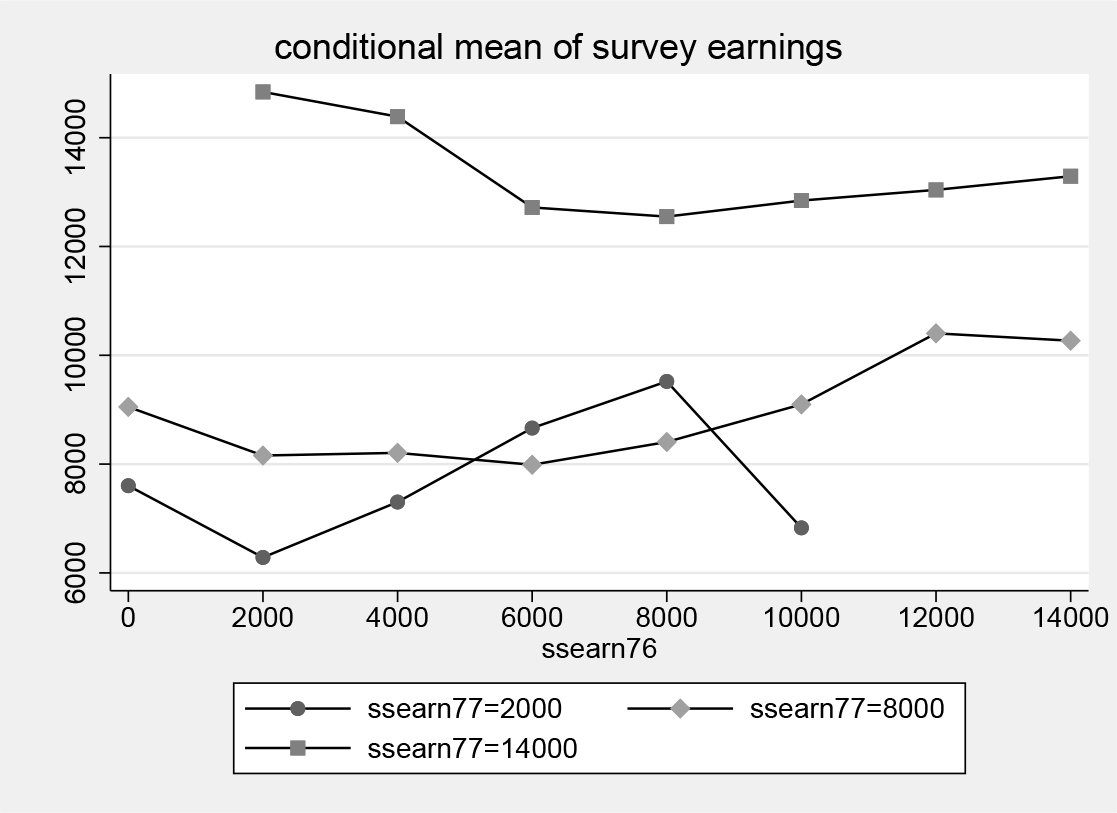
Nonparametric estimate of E(Y |X, Z), where Y is survey earnings in 1977 and X and Z are administrative earnings in 1977 and 1976, respectively. Bandwidths are chosen by cross-validation.

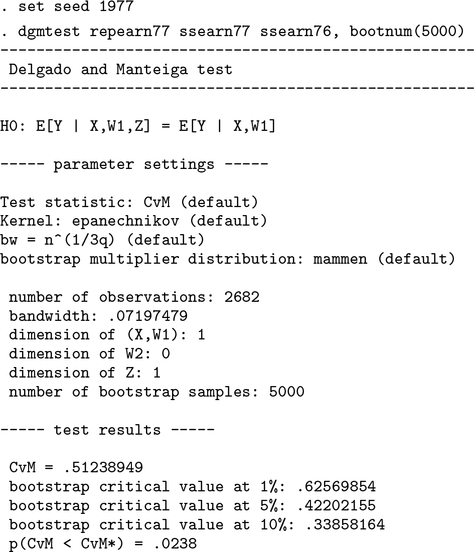
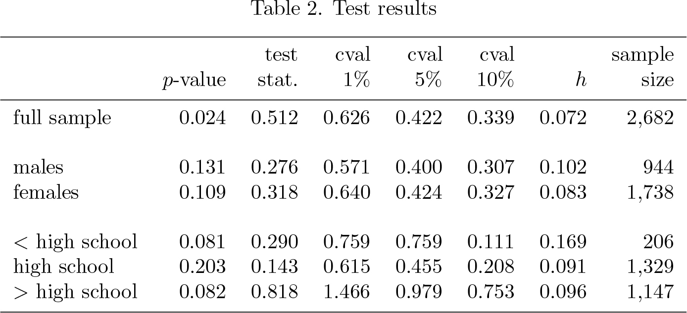
The test is performed using the new command, dgmtest, with its default settings, except we increase the number of bootstrap samples to 5,000:

The test produces a p-value of 0.0238, so we reject the null of no measurement error in administrative earnings at high confidence levels. Table 2 shows the test results for the full sample as well as for subsamples with the same gender and education. The p-values for the low and high education groups are about 8%, which is some evidence for the presence of measurement error but is weaker than in the full sample. For individuals in the middle education group, there is no evidence of measurement error. Similarly, we cannot reject the null on the subsamples of males and females. Of course, the sample sizes on the subsamples are significantly smaller than on the full sample, so it may be harder to reject the null for that reason.

Table 2.

Test results

	p-value	test stat.	cval 1%	cval 5%	cval 10%	h	sample size
full sample	0.024	0.512	0.626	0.422	0.339	0.072	2,682
males	0.131	0.276	0.571	0.400	0.307	0.102	944
females	0.109	0.318	0.640	0.424	0.327	0.083	1,738
< high school	0.081	0.290	0.759	0.759	0.111	0.169	206
high school	0.203	0.143	0.615	0.455	0.208	0.091	1,329
> high school	0.082	0.818	1.466	0.979	0.753	0.096	1,147

6 Conclusion

This article describes how to test for the presence of measurement error in covariates. While in linear regression models with classical measurement error, testing the null of no measurement error can be carried out using simple linear regression techniques, we introduce the dgmtest command, which implements a nonparametric test that does not rely on linearity nor on the measurement error (if there is any) to be classical.

The command is an implementation of the Delgado and González Manteiga (2001) test of conditional mean independence, a hypothesis that might be of interest in applications other than testing for the presence of measurement error.

Footnotes

7 Programs and supplemental materials

To install a snapshot of the corresponding software files as they existed at the time of publication of this article, type

Notes

References

Abowd

J. M.

Stinson

M. H.

2007. Estimating measurement error in SIPP annual job earnings: A comparison of census survey and SSA administrative data. In 2007 Federal Committee on Statistical Methodology (FCSM) Research Conference. National Center for Education Statistics, Institute of Education Sciences. https://nces.ed.gov/FCSM/pdf/2007FCSM_Stinson-VII-A.pdf.

Altonji

J. G.

1986. Intertemporal substitution in labor supply: Evidence from micro data. Journal of Political Economy 94: S176–S215. https://doi.org/10.1086/261403.

Arellano

Blundell

Bonhomme

2017. Earnings and consumption dynamics: A nonlinear panel data framework. Econometrica 85: 693–734. https://doi.org/10.3982/ECTA13795.

Attanasio

Cattan

Fitzsimons

Meghir

Rubio-Codina

2015. Estimating the production function for human capital: Results from a randomized control trial in Colombia. NBER Working Paper No. 20965, The National Bureau of Economic Research. https://doi.org/10.3386/w20965.

Attanasio

Meghir

Nix

2017. Human capital development and parental investment in India. Discussion Paper 1058, Yale University Economic Growth Center. https://doi.org/10.2139/ssrn.3002079.

Blundell

Horowitz

Parey

2017. Nonparametric estimation of a nonseparable demand function under the Slutsky inequality restriction. Review of Economics and Statistics 99: 291–304. https://doi.org/10.1162/REST_a_00636.

Blundell

Horowitz

J. L.

Parey

2012. Measuring the price responsiveness of gasoline demand: Economic shape restrictions and nonparametric demand estimation. Quantitative Economics 3: 29–51. https://doi.org/10.3982/QE91.

Bound

Brown

Mathiowetz

2001. Measurement error in survey data. In Handbook of Econometrics, ed. Heckman

J. J.

Leamer

E. E.

, 3705–3843. Vol. 5, 3705–3843. Amsterdam: Elsevier. https://econpapers.repec.org/bookchap/eeeeconhb/5.htm.

Card

1996. The effect of unions on the structure of wages: A longitudinal analysis. Econometrica 64: 957–979. https://doi.org/10.2307/2171852.

10.

Carroll

R. J.

Ruppert

Stefanski

L. A.

Crainiceanu

C. M.

2006. Measurement Error in Nonlinear Models: A Modern Perspective. Boca Raton, FL: Chapman & Hall/CRC.

11.

Chen

Hong

Nekipelov

2011. Nonlinear models of measurement errors. Journal of Economic Literature 49: 901–937. https://doi.org/10.1257/jel.49.4.901.

12.

Chesher

1990. On assessing the effect and detecting the presence of measurement error. Technical report, University of Bristol, UK.

13.

Chesher

1991. The effect of measurement error . Biometrika 78: 451–462. https://doi.org/10.1093/biomet/78.3.451.

14.

Chesher

Dumangane

Smith

R. J.

2002. Duration response measurement error. Journal of Econometrics 111: 169–194. https://doi.org/10.1016/S0304-4076(02)00103-3.

15.

Chetty

2012. Bounds on elasticities with optimization frictions: A synthesis of micro and macro evidence on labor supply. Econometrica 80: 969–1018. https://doi.org/10.3982/ECTA9043.

16.

Chetverikov

Wilhelm

2017. Nonparametric instrumental variable estimation under monotonicity. Econometrica 85: 1303–1320. https://doi.org/10.3982/ECTA13639.

17.

Cunha

Heckman

J. J.

Schennach

S. M.

2010. Estimating the technology of cognitive and noncognitive skill formation. Econometrica 78: 883–931. https://doi.org/10.3982/ECTA6551.

18.

Delgado

M. A.

González Manteiga

2001. Significance testing in nonparametric regression based on the bootstrap. Annals of Statistics 29: 1469–1507. https://doi.org/10.1214/aos/1013203462.

19.

Durbin

1954. Errors in variables. Review of the International Statistical Institute 22: 23–32. https://doi.org/10.2307/1401917.

20.

Fan

1996. Consistent model specification tests: Omitted variables and semiparametric functional forms. Econometrica 64: 865–890. https://doi.org/10.2307/2171848.

21.

Feng

2013. Misclassification errors and the underestimation of the US unemployment rate . American Economic Review 103: 1054–1070. https://doi.org/10.1257/aer.103.2.1054.

22.

Fitzenberger

Osikominu

Völter

2006. Imputation rules to improve the education variable in the IAB employment subsample. Schmollers Jahrbuch: Journal of Applied Social Science Studies / Zeitschrift für Wirtschaftsund Sozialwissenschaften 126: 405–436. https://doi.org/10.2139/ssrn.711044.

23.

Gozalo

1993. A consistent model specification test for nonparametric estimation of regression function models. Econometric Theory 9: 451–477. https://doi.org/10.1017/S0266466600007763.

24.

Groen

J. A.

2012. Sources of error in survey and administrative data: The importance of reporting procedures. Journal of Official Statistics 28: 173–198.

25.

Hahn

Hausman

2002. A new specification test for the validity of instrumental variables. Econometrica 70: 163–189. https://doi.org/10.1111/1468-0262.00272.

26.

Härdle

Mammen

1993. Comparing nonparametric versus parametric regression fits. Annals of Statistics 21: 1926–1947. https://doi.org/10.1214/aos/1176349403.

27.

Hausman

J. A.

1978. Specification tests in econometrics. Econometrica 46: 1251–1271. https://doi.org/10.2307/1913827.

28.

Heckman

Pinto

Savelyev

2013. Understanding the mechanisms through which an influential early childhood program boosted adult outcomes. American Economic Review 103: 2052–2086. https://doi.org/10.1257/aer.103.6.2052.

29.

Hoderlein

Holzmann

Kasy

Meister

2015. Erratum regarding “Instrumental variables with unrestricted heterogeneity and continuous treatment”. Boston College Working Papers in Economics 896, Boston College Department of Economics. https://ideas.repec.org/p/boc/bocoec/896.html.

30.

2008. Identification and estimation of nonlinear models with misclassification error using instrumental variables: A general solution. Journal of Econometrics 144: 27–61. https://doi.org/10.1016/j.jeconom.2007.12.001.

31.

2017. The econometrics of unobservables: Applications of measurement error models in empirical industrial organization and labor economics. Journal of Econometrics 200: 154–168. https://doi.org/10.1016/j.jeconom.2017.06.002.

32.

McAdams

Shum

2013. Identification of first-price auctions with non-separable unobserved heterogeneity. Journal of Econometrics 174: 186–193. https://doi.org/10.1016/j.jeconom.2013.02.005.

33.

Huang

Sun

White

2016. A flexible nonparametric test for conditional independence. Econometric Theory 32: 1434–1482. https://doi.org/10.1017/S0266466615000286.

34.

Kane

T. J.

Rouse

C. E.

1995. Labor-market returns to two-- and four-year colleges: Is a credit a credit and do degrees matter? American Economic Review 85: 600–614.

35.

Kane

T. J.

Rouse

C. E.

Staiger

1999. Estimating returns to schooling when schooling is misreported. NBER Working Paper No. 7235, The National Bureau of Economic Research. https://doi.org/10.3386/w7235.

36.

Kapteyn

Ypma

J. Y.

2007. Measurement error and misclassification: A comparison of survey and administrative data. Journal of Labor Economics 25: 513–551. https://doi.org/10.1086/513298.

37.

Kasy

2014. Instrumental variables with unrestricted heterogeneity and continuous treatment. Review of Economic Studies 81: 1614–1636. https://doi.org/10.1093/restud/rdu018.

38.

Mahajan

2006. Identification and estimation of regression models with misclassification. Econometrica 74: 631–665. https://doi.org/10.1111/j.1468-0262.2006.00677.x.

39.

Matzkin

R. L.

1994. Restrictions of economic theory in nonparametric methods. In Handbook of Econometrics, ed. Engle

R. F.

McFadden

D. L.

, 2523–2558. Vol. 4, 2523–2558. Amsterdam: Elsevier. https://doi.org/10.1016/S1573-4412(05)80011-X.

40.

Olley

G. S.

Pakes

1996. The dynamics of productivity in the telecommunications equipment industry. Econometrica 64: 1263–1297. https://doi.org/10.2307/2171831.

41.

Robinson

P. M.

1988. Root-n-consistent semiparametric regression. Econometrica 56: 931–954. https://doi.org/10.2307/1912705.

42.

Schennach

S. M.

2013. Measurement error in nonlinear models—A review. In Advances in Economics and Econometrics: Tenth World Congress, ed. Acemoglu

Arellano

Dekel

, 296–337, 296–337. Cambridge: Cambridge University Press. https://doi.org/10.1017/CBO9781139060035.009.

43.

Schennach

S. M.

2016. Recent advances in the measurement error literature. Annual Review of Economics 8: 341–377. https://doi.org/10.1146/annurev-economics-080315-015058.

44.

U.S. Census Bureau. 2009. March 1978 Current Population Survey/Social Security Summary Earnings. Ann Arbor, MI Inter-university Consortium for Political and Social Research. https://doi.org/10.3886/ICPSR09039.v3.

45.

Wilhelm

2015. Identification and estimation of nonparametric panel data regressions with measurement error. Working Paper CWP34/15, Centre for Microdata Methods and Practice, Institute for Fiscal Studies.https://doi.org/10.1920/wp.cem.2015.3415.

46.

Wilhelm

2018. Testing for the presence of measurement error. Working Paper CWP45/18, Centre for Microdata Methods and Practice, Institute for Fiscal Studies. https://doi.org/10.1920/wp.cem.2018.4518.

47.

D.-M.

1973. Alternative tests of independence between stochastic regressors and disturbances. Econometrica 41: 733–750. https://doi.org/10.2307/1914093.