Sage Journals: Discover world-class research

Abstract

Recentered influence functions (RIFs) are statistical tools popularized by Firpo, Fortin, and Lemieux (2009, Econometrica 77: 953–973) for analyzing unconditional partial effects on quantiles in a regression analysis framework (unconditional quantile regressions). The flexibility and simplicity of these tools have opened the possibility to extend the analysis to other distributional statistics using linear regressions or decomposition approaches. In this article, I introduce one function and two commands to facilitate the use of RIFs in the analysis of outcome distributions: rifvar() is an egen extension used to create RIFs for a large set of distributional statistics, rifhdreg facilitates the estimation of RIF regressions enabling the use of high-dimensional fixed effects, and oaxaca_rif implements Oaxaca–Blinder decomposition analysis (RIF decompositions).

Keywords

st0588 rifvar()rifhdreg rifsureg2 oaxaca_rif uqreg recentered influence functions unconditional partial effects unconditional quantile regression RIF regressions distributional statistics Oaxaca–Blinder RIF decomposition

1 Introduction

Influence functions (IFs) are statistical tools that have been used for analyzing the robustness of distributional statistics, or functionals, to small disturbances in data (Cowell and Flachaire 2007) or as a simplified strategy to estimate asymptotic variances of complex statistics (Cowell and Flachaire 2015; Deville 1999). More recently, Firpo, Fortin, and Lemieux (2009) suggested the use of IFs—specifically, recentered influence functions (RIFs)—as tools to analyze the impact that changes in the distribution of explanatory variables, X, has on the unconditional distribution of Y.

The method introduced by Firpo, Fortin, and Lemieux (2009) focused on the estimation of unconditional quantile regression (UQR), which allows the researcher to obtain partial effects of explanatory variables on any unconditional quantile of the dependent variable. The simplest version of this methodology, referred to as RIF–OLS (ordinary least squares), is easily implemented using the community-contributed command rifreg by the same authors. As part of their conclusions, the authors highlight the potential extensions of this strategy for analyzing other distributional statistics, as well as the potential usefulness for generalizing the traditional Oaxaca–Blinder (OB) decomposition for analyzing differences of outcome distributions across groups.¹

After its introduction, UQR became a popular method for analyzing and identifying the distributional effects on outcomes in terms of changes in observed characteristics in areas such as labor economics, income and inequality, health economics, and public policy. The potential simplicity and flexibility the methodology offers for the analysis of any distributional statistics also motivated subsequent research to expand the use of RIFs in the framework of regression analysis.

In a recently published article, Firpo, Fortin, and Lemieux (2018) discuss the application of RIF regressions for the variance and Gini coefficients, with emphasis on the generalization of the OB decomposition using RIFs.² Borgen (2016), building on the work of Firpo, Fortin, and Lemieux (2009), provides the command xtrifreg for the efficient estimation of UQR in the presence of a single high-dimensional fixed effect, but xtr ifreg cannot be used for other distributional statistics.

Cowell and Flachaire (2007), for their analysis on the sensitivity of inequality measures to the presence of extreme values, provide IFs for the most commonly used inequality indices, including the Atkinson index, generalized entropy index, and logarithmic variance index. Essama-Nssah and Lambert (2012), who discuss the use of RIF regressions and OB decompositions for the analysis of distributional changes, provide a large set of IFs and RIFs for distributional statistics relevant for policy analysis, including Lorenz and generalized Lorenz ordinates; Foster–Greer–Thorbecke (FGT) poverty indices; and Watts and Sen poverty indices. Most recently, Heckley, Gerdtham, and Kjellsson (2016) examine the use of RIFs for measures of health inequality, with emphases on bivariate rank-dependent concentration indices.

While RIF regressions and RIF decompositions have become important analytical tools in the empirical literature, there are only limited attempts to provide a simplified framework to allow the use of RIFs as a standard analytical tool. Within Stata, only the community-contributed command xtrifreg is readily available from the Stata Journal archives. The command rifireg is also available from the author’s website, but it is limited to the analysis of rank-dependent indices.³ The command that started it all, rifreg, is limited in the estimation of RIF statistics and is not available in the Statistical Software Components archives, although it can be accessed manually from the author’s website. Furthermore, while RIFs and reweighted regressions are broadly used for the generalization of the OB decomposition for statistics beyond the mean, existing commands can be used only to obtain decompositions based on a multistep process.⁴

In this article, I introduce one function and two commands that aim to facilitate the use of RIFs for regressions and decomposition analysis. The first function, rifvar(), is a byable plugin extension that works with egen and can be used to estimate the RIF for a large set of distributional statistics, such as those described in Firpo, Fortin, and Lemieux (2018); Essama-Nssah and Lambert (2012); Cowell and Flachaire (2007); and Heckley, Gerdtham, and Kjellsson (2016). The first command, rifhdreg, is a wrapper command for regress and reghdfe (Correia 2016) that in combination with rifvar() is used to estimate RIF regressions in the presence of high-dimensional fixed effects as well as inequality treatment effects. The second command, oaxaca_rif, is a wrapper around oaxaca (Jann 2008) that can be used to implement standard and reweighted OB decompositions (see Fortin, Lemieux, and Firpo [2011] and Firpo, Fortin, and Lemieux [2018]), implementing the multistep procedure described in Firpo, Fortin, and Lemieux (2018).

The rest of this article is structured as follows. Section 2 overviews what IFs are and how they are estimated. Section 3 introduces and explains the use of rifvar() to estimate RIF variables. Section 4 describes the use of rifhdreg for the estimation of standard RIF regressions, as well as for the estimation of inequality treatment effects. Section 5 describes the use of oaxaca_rif for the estimation of standard and reweighted decompositions using RIF decomposition. Section 6 concludes.

2 RIF and distributional statistics

2.1 Distributional statistics: Basics

When analyzing social welfare, inequality, poverty, or any other measure that describes the distributional characteristics of an outcome of interest, it is necessary to have access to one of the following pieces of information. The most common scenario is to have access to the full set of values corresponding to each observation in the population or sample. If the population or sample is of finite size n, it can be referred to as Y = [y ₁ , y ₂ ,…, y_n ], where each y_i is the outcome of interest (for example, income) of the ith person.

The second scenario is where we know the distribution of the outcome, based on either the cumulative distribution function (c.d.f.) or the probability distribution function (p.d.f.). Using the function F_Y (·) to refer to the c.d.f. and f_Y (·) to the p.d.f., the vector of information required for analyzing distributions can be more briefly written as a set of ordered pairs, F_Y = [{y, F_Y (y)}|y ∊ ℝ] or f_Y = [{y, f_Y (y)}|y ∊ ℝ], where y represents any real number (generally positive when referring to income).⁵ This simply means that if one has access to any of these vectors of information (Y, F_Y, f_y ), any distributional statistic can be derived.

Let us call v(·) a functional that uses all the information contained in Y, F_Y , or f_Y to estimate a distributional statistic of Y. This functional can be used to estimate statistics relevant to policy analysis, such as the mean, qth quantile, poverty indices, or inequality indices. To measure the impact a change in the distribution of income will have on the distributional statistic, one can simply compare the indices by swapping the c.d.f. from the observed distribution F_Y to the ex-post distribution G_Y .⁶ This can be written as follows:

Δ v = v (G_{Y}) - v (F_{Y})

Thus, Δv is the change in the distributional statistic generated by the change in distribution from F_y → G_y . This change can be as large as implying that everyone in the population receives a fixed transfer (shifting the function F_y (·) to the right)⁷ or as simple as having a new person (with random income) added to the sample, changing the rankings of everyone in the sample. The first scenario is a simplified example of what DiNardo, Fortin, and Lemieux (1996) used for analyzing changes in the distribution of wages. The second scenario is an exercise that can be used for understanding the definition of IFs and RIFs.

2.2 Estimations of IFs and RIFs: Gâteaux derivative

The thought experiment of adding a new person to a sample can also be considered as a case of data contamination in the original distribution, and (1) can be used to estimate the influence of this thought experiment on the statistic v. Standardizing the change in the statistic Δv with respect to some measure that quantifies the change of the distribution [Δ(G_Y − F_Y )] provides a quantification of the rate of change of the statistic v associated with the change of the distribution of Y from F_Y → G_Y .

Δ^{s} v = \frac{Δ v}{Δ (G_{Y} - F_{Y})} = \frac{v (G_{Y}) - v (F_{Y})}{Δ (G_{Y} - F_{Y})}

This process can be extended to measure Δ ^sv for an infinitesimally small change in the distribution function from F_Y → G_Y . This idea is what lies behind the Gâteaux derivative, which is a generalization of the directional derivative of a functional. The derivative is used to construct IFs, which can be used as measures of robustness of functionals to data outliers (Hampel 1974) and which facilitate the visualization of the structure of the distributional statistic as a function of the available data. Before we proceed to the formal definition of the IF, it would be useful to formalize the thought experiment just described.

Assume that the observation to be introduced in the sample has an income equal to y_i . Because this is the only element of that distribution, its c.d.f., H_y _i (y), can be characterized as follows:

\begin{array}{l} H_{y i} (y) = 0 \forall y < y_{i} \\ H_{y i} (y) = 1 \forall y \geq y_{i} \end{array}

This indicates that the distribution H_y _i puts mass only at the value y_i .⁸ With this definition, the distribution G_Y can be redefined as a combination of the distributions F_Y and H_y _i :

G_{Y} = (1 - ε) F_{Y} + ε H_{y i}

ε is strictly smaller than 1 but larger than 0. In other words, G_Y is the resulting distribution when the original distribution F_Y changes in the direction of H_y _i . This transformation can also be thought of as a contamination or perturbation of the distribution F_Y in the direction of H_y _i . Equation (2) also helps quantify the magnitude of the change in the distribution when moving from F_Y → G_Y (simply, ε). Figure 1 provides a graphical example of the changes we would observe as a result of this contamination of the distribution function F_Y .

Figure 1.

Comparison between original and contaminated distributions. note: The figure represents the contamination of the original distribution using ε = 0.2.

With this last concept in place, we can finally provide the formal definition of the IF:

IF {y_{i}, v (F_{Y})} = {lim}_{ε}_{\to 0} \frac{v {(1 - ε) F_{Y} + ε H_{y_{i}}} - v (F_{Y})}{ε} = \frac{\partial v (F_{Y} \to H_{y_{i}})}{\partial ε}

The IF is a directional derivative that shows the rate of change of the distributional statistic v caused by an infinitesimally small change in the distribution F_y in the direction of H_y _i . It can also be interpreted as the influence that observation y_i has on the estimation of the distributional statistic v. Take the distributional statistic mean as an example. The statistic and its IF are defined as follows:

\begin{array}{l} μ F_{y} = \int y d F_{y} \\ IF {y_{i}, v (F_{y})} = y_{i} - µ_{y} \end{array}

The IF indicates that if the distribution F_y were to be contaminated, adding more weight to observations with income y_i , the mean would change at a rate of y_i −µ_y . If the change in the distribution is ε, the change of the mean would be Δµ_y = ε×IF {y_i, v(F_Y )}. Note that the IF will be different for each point of reference y_i (contamination point) used for its estimation.

Instead of using the IF directly, Firpo, Fortin, and Lemieux (2009) propose using the recentered version of the statistics, the RIF, which is equivalent to the first two terms of the von Mises (1947) linear approximation of the corresponding distributional statistic v:

RIF {y_{i}, v (F_{Y})} = v (F_{Y}) + IF {y_{i}, v (F_{Y})}

This expression can be loosely interpreted as the relative contribution that observation y_i has on the construction of the statistic v. It can also be interpreted as an approximation of the statistic v after considering the influence of observation y_i . Returning to the example of the mean, the RIF(y_i, µ_F _y ) is defined as the observation itself, y_i , and it is easy to see that y_i is the relative contribution that observation i has on the construction of the mean.

As discussed in Firpo, Fortin, and Lemieux (2009); Cowell and Flachaire (2015); and Essama-Nssah and Lambert (2012), the IF and the RIF have the following properties:

\int IF {y, v (F_{Y})} d F_{Y} = 0

\int RIF {y, v (F_{Y})} d F_{Y} = v (F_{Y})

v (F_{y}) \sim N {v (F_{Y}), \frac{σ_{IF}^{2}}{N}}

σ_{IF}^{2} = \int IF {y, v (F_{Y})}^{2} d F_{Y}

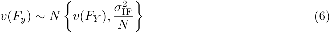
Equation (4) implies that the expected value of IFs constructed using all values of y_i is equal to 0. Because of this property, (5) implies that the expected value of RIFs is equal to the distributional statistic itself. Equations (6) and (7) indicate that the asymptotic variance of any statistic can be obtained by estimating the variance of the IF or the RIF based on sample data.

As shown in (3), choosing between IFs or RIFs as dependent variables has no impact in terms of regression analysis other than changes in the intercept in the case of RIF–OLS. This happens because IFs and RIFs are equivalent to each other up to a constant. The advantage of using RIFs, as shown in (5), is that one can use them to recover the underlying distributional statistics using simple averages. This property facilitates the interpretation of RIF regressions and enables the implementation of decomposition analysis.

3 Estimating RIFs: rifvar() egen function

The estimation of RIFs is a task of variable complexity. Some statistics have simple mathematical expressions that require few lines of code to define the corresponding RIF. The easiest example is the RIF for the mean because the RIF mean for any value y_i is simply itself. However, other statistics may require many intermediate steps to correctly define their corresponding RIFs.

The community-contributed command rifreg can be used to estimate RIF regressions and create their corresponding RIFs, but it is limited to the analyses of the variance, quantile, and Gini coefficient. If you are interested in analyzing other distributional statistics, I suggest the use of a new function called rifvar().⁹ This is a plugin command that adds new functions to the command egen, facilitating the estimation of RIFs for a large set of distributional statistics.¹⁰

The syntax of the command is as follows:

egen type newvar = rifvar( varname ) [if] [in] [, by( varname )

weight( varname ) seed( str ) RIF_options]

where varname is the variable being analyzed and newvar is the new variable name where the RIF will be stored, given the restrictions set by if, in, or both. All statistics allow for use of the option by( varname ), used to indicate the variables over which the RIF will be estimated (that is, sex or race group), and the option weight( varname ), used to indicate weights for the estimation of the RIFs. seed( str ) indicates a particular seed for replication of rank-dependent indices.

RIF_options allow the user to specify which distributional statistics are used to obtain the RIF statistic. Table 1 provides a detailed list of the statistics that are currently available for estimation. In appendix B, I provide a summary of performance simulation to show how well the RIF standard errors approximate the simulated standard errors for all of these statistics.

Table 1.

rifvar() RIF_options

Option	Description
mean	sample mean
var	variance
q( #p ) [kernel( kernel ) bw( # )]	pth quantile, where 0 < #p < 100; options kernel() and bw() are optional; default is kernel(gaussian) kernel; all kernel functions available for command kdensity are also allowed; † default is Silverman’s plug-in optimal bandwidth*
iqr( #p1 #p2 ) [kernel( kernel ) bw( # )]	interquantile range: q( #p2 )− q( #p1 ), where 0 < p ₁ ≤ p ₂ < 100; bw() and kernel() options are the same as for the quantile case
gini	Gini inequality index
cvar	coefficient of variation
std	standard deviation
iqratio( #p1 #p2 ) [kernel( kernel ) bw( # )]	interquantile ratio: q( #p2 )/q( #p1 ), where 0 < p ₁ ≤ p ₂ < 100; bw() and kernel() options are the same as for the quantile case
entropy( #a )	generalized entropy index with sensitivity parameter #a
atkin( #e )	Atkinson inequality index with inequality aversion #e > 0
logvar	logarithmic variance (different from variance of logarithms)
glor( #p )	generalized Lorenz ordinate at #p, where 0 < #p < 100
lor( #p )	Lorenz ordinate at #p, where 0 < #p < 100
ucs( #p )	share of income held by richest 1 − p%; 1 − lor( #p )
iqsr( #p1 #p2 )	interquantile share ratio: (1 − lor( #p2 ))/lor( #p1 ), where 0 < #p1 ≤ #p2 < 100
mcs( #p1 #p2 )	share of income held by people between #p1 and #p2: lor( #p2 )− lor( #p1 ), where 0 < #p1 < #p2 < 100
pov( #a ) pline( # \| varname )	FGT poverty index given sensitivity parameter #a; pov(0) returns the poverty head count, pov(1) returns the poverty gap, and pov(2) returns the poverty severity; FGT are defined based on the poverty line pline(), which can be a scalar (fixed poverty line) or a variable (variable poverty line)
watts( #povline )	Watts poverty index; requires a number or variable to define the poverty line
sen( #povline )	Sen poverty index; requires a number to define the poverty line
tip( #p ) pline( # )	three I’s of poverty (TIP) curve ordinate at #p for poverty line defined by pline( # ), where 0 < #p < 100
agini	absolute Gini
acindex( varname )	absolute concentration index using varname as the rank variable
cindex( varname )	concentration index using varname as the rank variable
eindex( varname ) lb( # ) ub( # )	Erreygers’s index using varname as the rank variable, with lower bound lb() and upper bound ub() and where lb() < ub()
arcindex( varname ) lb( # )	attainment relative concentration index using varname as the rank variable, with lower bound lb()
srindex( varname ) ub( # )	shortfall relative concentration index using varname as the rank variable, with upper bound ub()
windex( varname ) lb( # ) ub( # )	Wagstaff concentration index using varname as the rank variable, with lower bound lb() and upper bound ub() and where lb() < ub()
rifown( str ) rifopt( str )	these options allow the use of rifvar(), rifhdreg, and oaxaca_rif with other community-contributed RIFs for statistics that are not available in the current list; this may include the estimation of RIFs using numerical methods such as jackknife methods (Efron 1982) or analytical methods not yet programmed;¹¹ to use this, the new function should be implemented as an egen extension allowing for weight() and by() options, rifown() should contain the extension command name, and rifopt() should contain other options associated with the command; see file ghvarp().ado as an example

notes: † To use other kernel functions, the full kernel name should be used and not its abbreviation (for example, biweight instead of bi), with one exception: to request using the Epanechnikov kernel, one should use epan.

* In contrast, rifreg uses the default bandwidth from kdensity. This accounts for small differences in the estimation of unconditional quantile RIFs compared with rifreg. See the reghdfe help file for an example replicating rifreg results.

4 RIF regression: rifhdreg

4.1 Standard RIF regression

As previously indicated, IFs and RIFs have been used in statistics as tools for analyzing the robustness of statistics to outliers and as methods to draw statistical inferences from complex statistics (Cowell and Flachaire 2015; Deville 1999; Efron 1982; Hampel 1974). A recently popularized use by Firpo, Fortin, and Lemieux (2009); Heckley, Gerdtham, and Kjellsson (2016); and Essama-Nssah and Lambert (2012) is the estimation of RIF regressions.

Firpo, Fortin, and Lemieux (2009) use this strategy to estimate unconditional partial effects (UPE) of small changes in the distribution of the independent variables X on the distributional statistic v.¹² The authors use this strategy for the estimation of UQRs, using linear models as the easiest method for approximating these partial effects.¹³ Paraphrasing the original article, the estimation of RIF regressions can be described as follows.

Assume there is a joint distribution function dF_Y,X (y, x) = dF_Y _|X(y|X = x)dF_X (x) that determines the linear and nonlinear relationships between the dependent variable Y and all independent or exogenous variables X. Using this function, the p.d.f. and c.d.f. of the unconditional distribution of Y can be written as

d F_{Y} (y_{i}) = \int d F_{Y}_{| X} (y_{i} | X = x) d F_{X} (x)

F_{Y} (y_{i}) = \int F_{Y}_{| X} (y_{i} | X = x) d F_{X} (x)

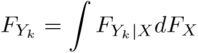
These expressions simply state that the unconditional c.d.f. (and p.d.f.) of Y can be obtained by integrating the conditional distributions F_Y _|X(·) (averaging) across all the realizations of X. It also implies that if one assumes F_Y _|X(y|x) remains constant, then changes in the distribution of X, say, from F_X → G_X , will translate in changes of the unconditional distribution of Y.

G_{Y} = \int F_{Y}_{| X} (y_{i} | X = x) d G_{X} (x)

Next assume that one is interested in analyzing the distributional statistic v(F_Y ). Based on (8) and (5), respectively, the statistic v can be rewritten as

v (F_{Y}) = \int RIF {y, v (F_{Y})} d F_{y}_{| X} (y | X = x) d F_{X} (x)

v (F_{Y}) = \int E [RIF {y, v (F_{Y})} | X = x] d F_{X} (x)

An intuitive interpretation of (11) is that any distributional statistics v can be written as the average of the RIFs weighted by the joint distribution dF_Y,X (y, x) = dF_y _|X(y|X = x)dF_X (x). Alternatively, (12) indicates that any distributional statistics can be obtained by averaging the conditional expectations of the RIFs with respect to X across the distribution dF_X (x). Equations (10) and (11) can also be used to state that if the distribution of the exogenous characteristics X changes, say, from F_X → G_X , assuming that the conditional distribution F_y _|X is constant, there will be a change in the unconditional distribution of Y from F_Y → G_Y that will translate into a change in the distributional statistic v(F_Y ) → v(G_Y ). Equation (12), which is used by Firpo, Fortin, and Lemieux (2009) to validate the use of RIFs in regression analysis, further suggests that the change in the distributional statistic caused by the change F_X → G_X can be approximated by

v (G_{Y}) - v (F_{Y}) = \int E [RIF {y, v (F_{Y})} | X = x] d (G_{X} - F_{X}) (x)

Equations (12) and (13) also imply that if E[RIF{y, v(F_y )}|X = x] can be modeled as a function of the distribution of X, those results can be used to estimate how changes in the distribution of X may affect the distributional statistic v.

Following Firpo, Fortin, and Lemieux (2009), the simplest approach to estimate RIF regressions is to assume a linear relationship between RIF{y, v(F_y )} and the explanatory variables X. Under this assumption, OLS can be used to fit a linear model to capture how small changes in the distribution of the independent variables X affect v(F_Y ). The difference with the standard OLS model is that RIF–OLS uses the RIF{y, v(F_Y )} for each observation y_i in the data as the dependent variable and regresses it against all the variables of interest:¹⁴

RIF {y, v (F_{Y})} = X^{'} β + ε_{i}, E (ε_{i}) = 0

While the use of OLS directly relates the RIF regression to standard regression analysis, some differences in the interpretation exist. In the standard OLS, the typical interpretation of the coefficients is that a one-unit increase in X will cause y to increase in β units (on average), everything else held constant. The interpretation from the RIF–OLS is slightly different. To obtain the UPE on the statistic v, one first needs to obtain unconditional expectations on both sides of (14):

v (F_{Y}) = E [RIF {y, v (F_{Y})}] = E (X^{'} β) + E (ε_{i}) = \bar{X}' β

$\bar{X}$ is the unconditional mean of X. From here, the UPE is given by

\frac{\partial v (F_{Y})}{\partial {\bar{X}}_{k}} = β_{k}

Based on (16), the correct interpretation of the UPE is that if the distribution of x_k changes such that its unconditional average increases by one unit $(Δ {\bar{X}}_{k} = 1)$ ,¹⁵ the distributional statistic is expected to change in β_k units. This interpretation identifies one weakness of using a linear regression that includes the explanatory variables linearly. It captures only the unconditional mean of the distribution of X. This can be easily mended by including higher-order polynomials and interactions that would better capture some of the nonlinear relationships across the independent variables and the RIF{y, v(F_Y )}. For example, assuming only one exogenous variable, the following specification could be applied:

RIF {y, v (F_{Y})} = β_{0} + β_{1} x + β_{2} {(x - \bar{X})}^{2} + ε_{i}

Taking the unconditional expectations, one obtains the following:

v (F_{Y}) = β_{0} + β_{1} \bar{X} + β_{2} E {{(X_{i} - \bar{X})}^{2}} = β_{0} + β_{1} \bar{X} + β_{2} Var (X)

The UPE is now a function of two moments of the unconditional distribution of X, the mean and the variance.¹⁶ An advantage of introducing the term ${(x - \bar{X})}^{2}$ , as opposed to simply adding x ², is that the UPE becomes a function of the mean and variance of X, which one can reasonably assume to change independently from each other.

The estimation of RIF regressions in Stata, under the linearity assumption, is easily implemented using the community-contributed commands rifreg (for Gini, variances, and quantiles), xtrifreg (for quantiles with one high-dimensional fixed effect), or rifireg (for rank-dependent variables). However, there are no commands for the estimation of RIF regressions for other distributional statistics or when two or more high-dimensional fixed effects need to be estimated.

For the estimation of RIF regressions under both scenarios, I introduce the command rifhdreg, which is a wrapper that uses the same two-step procedure used in rifreg. First, it estimates the corresponding RIF for each observation in the sample of interest for a specific distributional statistic using the previously introduced rifvar() function. Second, it uses the RIF as the dependent variable and fits a linear model using the official Stata command regress (when no fixed effects are used) or reghdfe (Correia 2016) (when fixed effects are used) to fit the RIF–OLS models. The syntax of the command is as follows:

rifhdreg depvar [indepvars] [if] [in] [weight], rif( RIF_options )

[retain( newvar ) replace abs( varlist ) iseed( str ) over( varname )

rwlogit( varlist ) rwprobit( varlist ) rwmlogit( varlist ) rwmprobit( varlist )

[ate| att| atu] scale( real ) svy regress options reghdfe options]

aweights, fweights, iweights, and pweights are allowed; see [U] 11.1.6 weight.

The main difference between the regress and reghdfe commands is that rifhdreg requires specifying the distributional statistic of interest with the rif( RIF_options ) option. See help rifhdreg for a description of all options.

rif( RIF_options ) specifies the statistic of interest, internally estimating the corresponding RIF in a first step. It uses the same syntax presented in table 1. For example, to estimate the RIF regression for the interquantile share ratio, one can type rifhdreg y x1 x2 x3, rif(iqsr(10 90)). rif() is required.

retain( newvar ) saves the internally constructed RIF for the restricted sample used in the regression under a new variable name.

replace, if used with retain(), replaces the internally constructed RIF if the newvar specified in retain() already exists.

abs( varlist ) identifies the fixed effects to be absorbed. Each variable listed here represents one set of fixed effects.

When abs( varlist ) is used, rifhdreg calls for reghdfe to fit the RIF–OLS model, and all options in reghdfe are available. Otherwise, it uses regress to fit the model, allowing for all regress options.¹⁷

iseed( str ) is used for the creation of an auxiliary random variable that can be used to obtain replicable estimates for rank-dependent indices when ties exist.

scale( real ) provides a value for rescaling the dependent variable. It may be useful for statistics like the Lorenz ordinate or quantile shares, which are measures that fall between 0 and 1. In those cases, using scale(100) would change the scale to be between 0–100. The default is scale(1) (no rescaling).

rifhdreg reports OLS asymptotic standard errors by default, but one can request other standard errors allowed in regress or reghdfe commands, for example, robust and clustered standard errors. Simple survey design standard errors are also available via the option svy ¹⁸ when no fixed effects are included.

Based on the recommendation provided in Firpo, Fortin, and Lemieux (2009) and the simulations presented in appendix A, bootstrap standard errors should be used when the statistics of interest are the unconditional quantiles or statistics related to unconditional quantiles, or at the very least, robust standard errors should be requested.¹⁹ The reason for this is that RIFs for unconditional quantiles require the estimation of density functions, which are taken as known parameters for the estimation of asymptotic standard errors. For the correct estimation of bootstrap standard errors, one should use the bootstrap prefix before the rifhdreg command. One can also use the communitycontributed command bs4rw (Kolenikov 2010) for the estimation of bootstrap standard errors allowing for complex survey design.²⁰

To illustrate the use of this command for the estimation of RIF regressions, table 2 provides the output of RIF regressions for selected distributional statistics, using an excerpt from the Swiss Labor Market Survey available online.²¹ For simplicity, only years of education, years of experience, years of job tenure, sex, and single status are used as explanatory variables. At the bottom of the table, the average RIF is reported as a reference point for the UPE interpretation. Three forms of standard errors are reported: the default or OLS standard errors, robust standard errors, and bootstrap standard errors based on 500 repetitions. The estimation corresponding to the Gini rescales the parameters by 100 to help with the interpretation of the estimated coefficients. All interpretations are given in relative terms with respect to the current levels of inequality to make the results comparable across inequality measures.

Table 2.

Determinants of wage inequality

	lnwage iqr(90 10)	wage iqratio(90 10)	wage iqsr(10 90)	wage Gini × 100	lnwage Variance
Years of education	−0.0154	−0.0542	−0.8580	−0.5715	−0.0357
Default	(0.0127)	(0.0375)	(0.1760)*	(0.2802)+	(0.0082)*
Robust	(0.0154)	(0.0453)	(0.2220)*	(0.3255)∧	(0.0117)*
Bootstrap	(0.0188)	(0.0543)	(0.2970)*	(0.3391)∧	(0.0114)*
Years of experience	−0.0263	−0.0774	−0.2690	−0.4888	−0.0129
Default	(0.0046)*	(0.0135)*	(0.0636)*	(0.1010)*	(0.0030)*
Robust	(0.0046)*	(0.0135)*	(0.0614)*	(0.1243)*	(0.0026)*
Bootstrap	(0.0052)*	(0.0159)*	(0.0758)*	(0.1267)*	(0.0026)*
Years of job tenure	0.0041	0.0118	0.0490	0.0734	0.0017
Default	(0.0048)	(0.0141)	(0.0662)	(0.1052)	(0.0031)
Robust	(0.0047)	(0.0137)	(0.0533)	(0.1019)	(0.0024)
Bootstrap	(0.0049)	(0.0144)	(0.0510)	(0.0973)	(0.0022)
Is female	0.0438	0.1440	1.4370	3.5025	0.0544
Default	(0.0614)	(0.1810)	(0.8520)∧	(1.3534)*	(0.0396)
Robust	(0.0613)	(0.1800)	(0.8280)∧	(1.3000)*	(0.0368)
Bootstrap	(0.0671)	(0.1970)	(0.8850)	(1.3531)*	(0.0381)
Age	0.0137	0.0391	−0.0222	0.1806	0.0014
Default	(0.0047)*	(0.0138)*	(0.0651)	(0.1035)∧	(0.0030)
Robust	(0.0050)*	(0.0146)*	(0.0819)	(0.1515)	(0.0037)
Bootstrap	(0.0056)+	(0.0165)+	(0.0793)	(0.1466)	(0.0035)
Is single	−0.0637	−0.1810	0.9320	0.0506	0.0439
Default	(0.0709)	(0.2090)	(0.9840)	(1.5627)	(0.0457)
Robust	(0.0617)	(0.1810)	(0.7140)	(1.4090)	(0.0282)
Bootstrap	(0.0652)	(0.1920)	(0.7720)	(1.3658)	(0.0286)
cons	1.0230	2.9170	18.9000	28.3451	0.7550
Default	(0.1980)*	(0.5830)*	(2.7410)*	(4.3541)*	(0.1270)*
Robust	(0.2280)*	(0.6710)*	(3.5830)*	(4.9969)*	(0.1640)*
Bootstrap	(0.2790)*	(0.8080)*	(4.6740)*	(4.6601)*	(0.1490)*
Avg. RIF	1.0595	2.8844	6.0285	24.6030	0.2818
N	1434	1434	1434	1434	1434

note: Standard errors in parentheses.

∧ p < 0.1

+ p < 0.05

* p < 0.01

In terms of the standard errors, as expected, OLS standard errors tend to be smaller than robust standard errors for most of the explanatory variables across all models. Bootstrap standard errors, which Firpo, Fortin, and Lemieux (2009) indicate to be the most appropriate for statistical inference, are considerably larger for the regressions that involve quantile statistics. Consistent with the results from the RIF simulations, however, bootstrap errors are similar to the robust standard errors for regressions that focus on the Gini coefficient and variance of log wages.²²

All models have consistent results with different insights for different measures of wage inequality. If the average number of years of education in the population were to increase by one year, the predicted Gini coefficient would drop by just over half a point (2.32% in relative terms), the variance of log wage would drop by 12.7% (−0.036/0.2818), and the ratio of wages held by the richest 10% compared with the poorest 10% by 14.2% (−0.86/6.0285). The log wage gap and wage ratio between the 90th quantile and 10th quantile may also decline, but the change is not statistically significant. Increasing the number of years of experience seems to reduce wage inequality, whereas aging of the population may have a small effect by increasing the gap between the top and bottom of the wage distribution. This is not observed for other statistics that look across the wage distribution.

Perhaps one of the most challenging variable types to interpret in terms of UPE is categorical variables. On one hand, because RIF and standard RIF regressions are meant to estimate the impact of small changes in the distribution of the independent variables, one should not interpret the coefficients of categorical variables as changes from 0 to 1. Otherwise, the exercise implies a large change in the distribution of the categorical variable, from 0% of observations being classified in that group to 100% being classified in that group, which may introduce a large bias on the predicted UPE.²³ On the other hand, based on (15) and (16), one should analyze the UPE as deviations from the observed unconditional averages. For example, if the proportion of women in the population would increase by 10 percentage points, from 47.6% as currently observed to 57.6%, the ratio of wages held by the richest 10% to the poorest 10% would increase by 2.3% (1.437/6.0285 × 0.1) and the predicted Gini coefficient would increase by 1.4% (3.502/24.603 × 0.1).

To illustrate the capabilities of the rifhdreg command to estimate RIF regressions allowing for multiple fixed effects, the model of table 2 is refit, including occupation, age, and single status as fixed effects.²⁴ The results are reported in table 3 using robust and bootstrap standard errors.

Table 3.

Determinants of wage inequality

	lnwage iqr(90 10)	wage iqrtio(90 10)	wage iqsr(10 90)	wage Gini	lnwage Variance
Years of education	0.0280	0.0772	0.1490	0.0072	0.0028
Robust	(0.0164)∧	(0.0479)	(0.2110)	(0.0037)+	(0.0120)
Bootstrap	(0.0170)	(0.0509)	(0.2040)	(0.0036)+	(0.0115)
Years of experience	−0.0215	−0.0632	−0.1650	−0.0033	−0.0076
Robust	(0.0047)*	(0.0136)*	(0.0574)*	(0.0012)*	(0.0025)*
Bootstrap	(0.0050)*	(0.0151)*	(0.0623)*	(0.0011)*	(0.0025)*
Years of job tenure	0.0006	0.0010	−0.0440	−0.0005	−0.0023
Robust	(0.0047)	(0.0137)	(0.0574)	(0.0011)	(0.0025)
Bootstrap	(0.0050)	(0.0147)	(0.0566)	(0.0011)	(0.0024)
Is female	0.0790	0.2490	2.0150	0.0355	0.0863
Robust	(0.0627)	(0.1840)	(0.7540)*	(0.0119)*	(0.0356)+
Bootstrap	(0.0698)	(0.2040)	(0.8010)+	(0.0121)*	(0.0352)+
N	1434	1434	1434	1434	1434

notes: Standard errors in parentheses.

All models include age, occupation, and single status fixed effects.

∧ p < 0.1

+ p < 0.05

∗ p < 0.01

In this example, controlling for the age and occupation fixed effects is effectively controlling for all linear and nonlinear relationships these variables have with the dependent variable. In this case, the results suggest that increasing the average number of years of education by one year may increase inequality by about 2.9% regardless of the measure of inequality and holding everything else constant. In contrast, if the number of years of experience increases by one unit, inequality would decline between 1.3% to 2.7%, depending on the inequality measure. Also consistent with the results in table 2, if the proportion of women in the sample increases by 10 percentage points, then inequality measured by the interquantile share ratio, the Gini coefficient, and the log variance will increase by 1.4% to 3.3%.

4.2 Inequality treatment effects: Advanced options

As previously described, standard RIF regressions should not be used to estimate the effect of large changes in the distribution of the independent variables, particularly when considering categorical variables. In fact, Essama-Nssah and Lambert (2012) emphasize that one of the main weaknesses of RIF regressions is that coefficients provide only local approximations of the effect of changes in the distribution of the independent variables.

In an attempt to address this weakness, other studies in the literature, including Rothe (2010), Donald and Hsu (2014), Firpo and Pinto (2016), and Firpo, Fortin, and Lemieux (2018), have proposed methodologies for the estimation of what Firpo and Pinto (2016) call inequality treatment effects. In essence, these methodologies use parametric or nonparametric strategies to obtain inverse probability weights that can be used to identify counterfactual distributions and identify the treatment effects on distributional statistics. Paraphrasing Firpo and Pinto (2016), the estimation of inequality treatment effects can be described as follows.

Assume there is a joint distribution function $F_{Y_{1}}_{, Y_{0}, X, T} (\cdot)$ that characterizes the relationships between the potential outcomes Y ₁ and Y ₀, a set of exogenous explanatory variables X, and a binary treatment T . If potential outcomes could be observed for everyone in the population, inequality treatment effects could be estimated by simply comparing the distributional statistic of interest v for both potential outcomes as follows:

Δ v = v_{1} - v_{0} = v (F_{Y}_{_{1}}) - v (F_{Y_{0}})

$F_{Y_{1}}$ and $F_{Y_{0}}$ represent the unconditional cumulative distributions of the potential outcomes.

Empirically, both potential outcomes are never fully observed. Instead, one is able to observe only the realized outcome depending on whether an individual is in part of the treated group:

Y = T \times Y_{1} + (1 - T) Y_{0}

According to Firpo and Pinto (2016), under the assumption that the distribution of potential outcomes Y ₁ and Y ₀ are independent from treatment assignment when conditioning on observed characteristics X (unconfoundedness) and that there are enough observations so that it is possible to find individuals with similar observed characteristics X in both groups (overlapping support), treatment effects, as defined in (18), can be identified using the following procedure.

Recall from (9) that the unconditional c.d.f. can also be written by integrating (averaging) the conditional distributions with respect to X and T :

F_{Y k} = \int F_{Y_{k}}_{| X, T} d F_{X, T}

Based on the unconfoundedness assumption, we know that $F_{Y_{k}}_{| X, T = 1} = F_{Y_{k}}_{| X, T = 0} = F_{Y_{k}}_{| X}$ . This implies that (19) can be written solely in terms of the distribution of X:

F_{Y_{k}} = \int F_{Y_{k}}_{| X} d F_{X}

As indicated before, the full distribution of the potential outcomes is never observed. Instead, only the distribution of the realized outcome after treatment has been assigned is available. Using the unconfoundedness assumption again, the observed distribution of the outcome among individuals who are treated and untreated can be defined as

F_{Y_{k}}_{| T = k} = \int_{i \in k} F_{Y_{k}}_{| X} d F_{X}_{| T = k} for k = 0, 1

which considers only observations that are in the treated or untreated group. Because the distribution implied by (20) is fully observed, it can be used to identify $F_{_{Y k}}$ using

{\hat{F}}_{Y_{k}} = \int_{i \in k} F_{Y_{k}}_{| X} ω_{k} (x) d F_{X | T = k}

where ω_k (x) is a weighting factor such that ω_k (X)dF_X _|T _=k resembles the unconditional distribution dF_X . This weighting factor can be identified as follows:

\begin{array}{l} ω_{k} (x) = \frac{d F_{X}}{d F_{X | T = k}} = d F_{X} \times \frac{P (T = k)}{P (T = k | X = x) d F_{X}} = \frac{P (T = k)}{P (T = k | X = x)} \\ ω_{k} (x) = \frac{P (T = 1)}{P (T = 1 | X = x)} and ω_{0} (x) = \frac{1 - P (T = 1)}{1 - P (T = 1 | X = x)} \end{array}

When k = 1, P (T = 1) is the overall probability that an observation is assigned to the treatment group, and P (T = 1|X = x) is the probability that an observation is assigned to the treatment group conditional on the observed characteristics. Following Firpo and Pinto (2016), this probability can be estimated using parametric methods such as probit or logit models, as well as other semiparametric or nonparametric methods.

Once the weights ω ₁(x) and ω ₀(x) have been obtained, the treatment effects defined in (18) can be estimated as follows:

\begin{array}{l} Δ \hat{v} = v ({\hat{F}}_{Y_{1}}) - v ({\hat{F}}_{Y}_{_{0}}) \\ Δ \hat{v} = v {\int_{i \in 1} F_{y}_{| X} {\hat{ω}}_{1} (x) d F_{X}_{| T = 1}} - v {\int_{i \in 0} F_{y}_{| X} {\hat{ω}}_{0} (x) d F_{X}_{| T = 0}} \end{array}

Firpo and Pinto (2016) denominate this as an overall treatment effect, and it is similar to the estimation of average treatment effects.²⁵ While $v ({\hat{F}}_{Y_{1}})$ and $v ({\hat{F}}_{Y_{0}})$ can be obtained by simply estimating the statistic of interest v using the reweighting factors ${\hat{ω}}_{1} (X)$ and ${\hat{ω}}_{0} (X)$ over the sample of treated and untreated observations, they can also be estimated using RIFs:

v ({\hat{F}}_{Y_{k}}) = \int_{i \in k} E [RIF {y, v ({\hat{F}}_{Y_{k}})} | X = x] {\hat{ω}}_{k} (x) d F_{X}_{| T = k} (x)

Based on (21), treatment effects can be estimated using RIF regressions, fitting the model

T \times RIF {y, v ({\hat{F}}_{Y_{1}})} + (1 - T) \times RIF {y, v ({\hat{F}}_{Y_{0}})} = b_{0} + b_{1} T + ε

using weighted least squares with weights equal to $\hat{ω} (x) = T {\hat{ω}}_{1} (x) + (1 - T) {\hat{ω}}_{0} (x)$ , and where the dependent variable is constructed by combining the RIFs based on the reweighted cumulative distribution functions ${\hat{F}}_{Y_{1}}$ and ${\hat{F}}_{Y_{0}}$ , which are estimated separately for observations in the treated and untreated groups.

Applying conditional expectations with respect to T on both sides of (22) and taking the derivative with respect to T, it is easy to see that the overall inequality treatment effect (average treatment effect) is equal to b ₁:²⁶

\begin{array}{l} T \times E [RIF {y, v ({\hat{F}}_{Y_{1}})} | T = 1] + (1 - T) \\ \times E [RIF {y, v ({\hat{F}}_{Y_{0}})} | T = 0] = b_{0} + b_{1} T \\ T \times v ({\hat{F}}_{Y_{1}}) + (1 - T) \times v ({\hat{F}}_{Y_{0}}) = b_{0} + b_{1} T \\ v ({\hat{F}}_{Y_{1}}) - v ({\hat{F}}_{Y_{0}}) = b_{1} \end{array}

The advantage of using RIF regressions for the estimation of treatment effects using specifications similar to (22) is that one can also control for differences in the distribution of characteristics directly by including them as control variables in the model specification. In addition, if the variable T has more than two categories, (22) can still be estimated by using RIFs constructed using all categories in T , and coefficients associated with T can be interpreted as treatment effects, while coefficients of other variables would be interpreted as UPE that are averaged across the distributions defined by T .²⁷

The command rifhdreg offers three advanced options that can be used to estimate inequality treatment effects using models like the one just described.

The first option is over( varname ). It is used to specify a variable over which the RIF will be estimated, just as the option by() is used in the rifvar() function. For example, if one uses the command rifhdreg y x i.T, over(T) rif(q(10)), where T is a categorical variable, the command will first estimate the 10th quantile RIF for y for all groups defined by T and use that as the dependent variable in the regression model. When the variable used in over( varname ) is binomial, the regression can also be seen as the OLS alternative to OB decomposition.

rwlogit( varlist ) and rwprobit( varlist ) are options used to specify the estimation of the reweighting factors ω_k (x) using a logit or probit model and using the variable specified in over() as the dependent variable. These options can be used to estimate distributional treatment effects under the exogeneity assumption, using weighted least squares based on (22), as described in Firpo and Pinto (2016). When either of these options is used, the user should also specify the type of treatment effect that will be estimated. The options are average treatment effect, ate (default); treatment effect on the treated, att; or treatment effect on the untreated, atu. When using this option, a new variable will be created under the name wipw containing the estimated ω(X). Using rwlogit() or rwprobit() in combination with the inclusion of independent variables in the model specification can be compared with the inverse-probability weighted regression adjustment estimator of treatment effects.

rwmlogit( varlist ) and rwmprobit( varlist ) are options used to specify the estimation of the reweighting factors ω_k (x) using a multinomial logit or multinomial probit model, using the variable specified in over() as the dependent variable. These options can be used to estimate distributional multivalued treatment effects under the exogeneity assumption using weighted least squares. When using any of these options, only the average treatment effect (ate) can be estimated.

To provide an example showing the estimation of inequality treatment effects using rifhdreg‘s advanced options, table 4 (below) provides the estimated overall treatment effects following the same specification of the models presented in table 2, but where the corresponding RIFs are calculated over the treatment variable being a woman. Four specifications are used: i) no controls, ii) no controls but using the reweighting adjustment (IPW), iii) adding controls as in table 2, but without the reweighting adjustment, and iv) adding both controls and the reweighting adjustment. The conditional probabilities of treatment are estimated with a probit model that uses the same variables used in the outcome model.

Table 4.

Estimation of overall treatment effects of gender

Treatment effect: Female	No controls	No controls +IPW	Controls	Controls +IPW
Mean (lnwage)	−0.1735	−0.1400	−0.1290	−0.1376
Robust	(0.0279)*	(0.0290)*	(0.0247)*	(0.0251)*
Bootstrap	(0.0271)*	(0.0243)*	(0.0238)*	(0.0245)*
10th quantile (lnwage)	−0.2486	−0.2220	−0.1977	−0.2191
Robust	(0.0448)*	(0.0489)*	(0.0441)*	(0.0463)*
Bootstrap	(0.0487)*	(0.0501)*	(0.0484)*	(0.0499)*
90th quantile (lnwage)	−0.1386	−0.1233	−0.1270	−0.1219
Robust	(0.0376)*	(0.0413)*	(0.0391)*	(0.0394)*
Bootstrap	(0.0503)*	(0.0546)+	(0.0512)+	(0.0544)+
iqr(90 10) (lnwage)	0.1100	0.0987	0.0710	0.0973
Robust	(0.0544)+	(0.0596)∧	(0.0572)	(0.0588)∧
Bootstrap	(0.0697)	(0.0767)	(0.0725)	(0.0764)
iqratio(90 10) (wage)	0.3028	0.2733	0.1927	0.2690
Robust	(0.1567)∧	(0.1747)	(0.1646)	(0.1723)
Bootstrap	(0.2024)	(0.2198)	(0.2087)	(0.2189)
iqsr(90 10) (wage)	2.3540	1.5549	1.4275	1.5335
Robust	(0.9301)+	(0.8401)∧	(0.8904)	(0.8141)∧
Bootstrap	(0.9602)+	(0.8434)∧	(0.8723)	(0.8481)∧
Gini (wage)	4.6632	3.7194	3.4512	3.7124
Robust	(1.3548)*	(1.3290)*	(1.3331)*	(1.3204)*
Bootstrap	(1.4118)*	(1.3778)*	(1.3810)+	(1.3845)*
Variance (lnwage)	0.0957	0.0599	0.0540	0.0590
Robust	(0.0381)+	(0.0370)	(0.0366)	(0.0361)
Bootstrap	(0.0392)+	(0.0376)	(0.0383)	(0.0378)
N	1434	1434	1434	1434

note: Robust and bootstrap standard errors, based on 500 repetitions, in parentheses. All models provide estimations for overall treatment effects of gender. Four specifications are used, combining controls and reweighting adjustment.

∧ p < 0.1

+p < 0.05

∗p < 0.01

The first column in table 4 provides the estimation of overall treatment effects without using any controls. These results provide an estimate of the raw distributional gap between women and men and are most likely to provide biased estimates for treatment effects. Overall, this result indicates that women earn on average about 17.4% lower wages, with a larger gap (24.8%) at the 10th quantile but a somewhat smaller gap (13.9%) at the 90th quantile. This column also suggests that there is somewhat higher wage inequality among women.

The second, third, and fourth columns, which control for differences in characteristics in various ways, suggest that the negative treatment effects of gender at the means and the 10th and 90th quantiles are smaller than the raw gaps would suggest, albeit only marginally. In terms of inequality, after controlling for other characteristics, the results suggest that the treatment effect of gender may not increase inequality as much as the raw gender gap suggests. The three methods used to control for differences in characteristics provide similar results, with the largest differences observed for the treatment effect on the Gini coefficient and the interquantile ratio.

5 RIF decomposition: oaxaca_rif

As previously described, one of the main advantages of standard RIF regressions described in section 4.1 is that they can be easily used to analyze how small changes in the distribution of independent characteristics will affect the distributional statistic v. Furthermore, the modified RIF regression described in section 4.2 can also be used to estimate inequality treatment effects caused by an exogenous treatment.

However, there is often interest in analyzing what factors explain the differences in the distribution between two groups. The OB decomposition is one of the most extensively used methodologies in labor economics that aims to analyze outcome differences between two groups (Blinder 1973; Oaxaca 1973). These differences are characterized as functions of differences in characteristics (composition effect) and differences in coefficients associated with those characteristics (wage structure effect).

While the original methodology was created to analyze differences of outcome means, several articles that followed provided extensions and refinements to extend the analysis to other distributional statistics (see Fortin, Lemieux, and Firpo [2011] for a review). Additionally, under the assumptions of conditional independence (unconfoundedness) and overlapping support, the aggregate structure effect can be identified and interpreted as a treatment effect.²⁸

Firpo, Fortin, and Lemieux (2018) describe the use of RIF regressions, in combination with a reweighted strategy (DiNardo, Fortin, and Lemieux 1996), as a feasible methodology for decomposing differences in distributional statistics beyond the mean. This is referred to as RIF decomposition. This methodology has three advantages compared with other strategies in the literature: the simplicity of its implementation, the possibility of obtaining detailed contributions of individual covariates on the aggregate decomposition,²⁹ and the possibility of expanding the analysis to any statistic for which a RIF can be defined. This strategy can be described as follows.

Assume there is a joint distribution function that describes all relationships between the dependent variable Y, the exogenous characteristics X, and the categorical variable T that identifies the group membership of the population (f_Y,X,T ). The cumulative distribution of Y conditional on T can be written as

F_{Y}_{| T = k} = \int F_{Y}_{| X, T = k} d F_{X}_{| T = k}

To analyze the differences between groups 0 and 1, the cumulative conditional distribution of Y can be used to calculate the gap in the distributional statistic v:

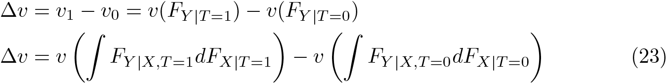
\begin{array}{l} Δ v = v_{1} - v_{0} = v (F_{Y} {_{|}}_{T}_{= 1}) - v (F_{Y} {_{|}}_{T}_{= 0}) \\ Δ v = v (\int F_{Y}_{| X, T = 1} d F_{X}_{| T = 1}) - v (\int F_{Y}_{| X, T = 0} d F_{X}_{| T = 0}) \end{array}

From (23), it is easy to see that differences in the statistics of interest Δv will arise because of differences in the distribution of X (dF_X _|T ₌₁ ≠ dF_X _|T ₌₀) or because of differences in the relationships between Y and X (dF_Y _|X,T ₌₁ ≠ dF_Y _|X,T ₌₀). In the context of the standard OB decomposition, this is equivalent to comparing differences in average characteristics and differences in coefficients.

To identify how important differences in characteristics (composition effect) and differences in coefficients (wage structure effect) are for explaining the overall gap in the distributional statistic v, it is necessary to create a counterfactual scenario. Define the counterfactual statistic v_c as follows:

v_{c} = v (F_{Y}^{c}) = v (\int F_{Y}_{| X, T = 0} d F_{X}_{| T = 1})

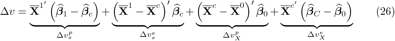
Using this counterfactual, the gap in the distribution statistic v can be disaggregated into two components:

Δ v = \underset{Δ v_{S}}{\underset{︸}{v_{1} - v_{c}}} + \underset{Δ v_{X}}{\underset{︸}{v_{c} - v_{0}}}

Δv_X reflects the gap attributed to differences in characteristics, and Δv_S reflects the differences attributed to the relationships between Y and X (structure effect). The difficulty of this strategy lies in the identification of the counterfactual statistic v_c because the combination of characteristics and outcomes is not observed in the data. Based on the review in Fortin, Lemieux, and Firpo (2011), two broad strategies have been suggested for the identification of the counterfactual statistic v_c . The first strategy follows the standard OB decomposition, using linear regressions and their approximations to identify v_c . Specifically, following (15), separate RIF regressions can be estimated for each group, so the counterfactual statistic can be identified as follows:

\begin{array}{l} v_{1} = E [RIF {y, v (F_{Y} {_{|}}_{T}_{= 1})}] = {\bar{X}}^{1}^{'} {\hat{β}}^{1} \\ v_{0} = E [RIF {y, v (F_{Y} {_{|}}_{T}_{= 0})}] = {\bar{X}}^{0}^{'} {\hat{β}}^{0} \\ v_{c} = {\bar{X}}^{1'} {\hat{β}}^{0} \end{array}

This alternative mirrors the standard OB decomposition, where $Δ v_{X} = {({\bar{X}}^{1} - {\bar{X}}^{0})}^{'} β^{0}$ and $Δ v_{S} = {\bar{X}}^{1'} ({\hat{β}}^{1} - {\hat{β}}^{0})$ . The main disadvantage of this strategy, discussed in Barsky et al. (2002) in the context of conditional means, is that the counterfactual statistic v_c may be incorrectly identified if the model is misspecified³⁰ or if the local approximation obtained using RIF cannot be extended beyond local extrapolations. The alternative is to use a semiparametric reweighting approximation, as discussed in Barsky et al. (2002) and DiNardo, Fortin, and Lemieux (1996), to identify the counterfactual distribution F_Y _|X,T ₌₀ dF_X _|T ₌₁ based on the observed data. This procedure can be described as follows.

The problem of identifying the counterfactual scenario is that the distribution of outcomes and characteristics that the counterfactual distribution $F_{Y_{0}}$ implies cannot be directly observed. However, from an abstract point of view, it is possible to obtain an approximation for the counterfactual distribution by multiplying the observed distribution of characteristics dF_X _|T ₌₀ with a factor ω(X), so it resembles the distribution dF_X _|T ₌₁:

F_{Y}^{C} = \int F_{Y}_{| X, T = 0} d F_{X}_{| T = 1} ≅ \int F_{Y}_{| X, T = 0} d F_{X}_{| T = 0} ω (X)

Using the Bayes rule, the reweighting factor ω(X) can be identified as follows:

\begin{matrix} ω (X) = \frac{d F_{X | T = 1}}{d F_{X | T = 0}} = \frac{d F_{T = 1 | X} d F_{X}}{d F_{T = 1}} \frac{d F_{T = 0}}{d F_{T = 0 | X} d F_{X}} = \frac{d F_{T = 0}}{d F_{T = 1}} \frac{d F_{T = 0 | X}}{d F_{T = 0 | X}} \\ = \frac{1 - P}{P} \frac{P (T = 1 | X)}{1 - P (T = 1 | X)} \end{matrix}

p is the proportion of people in group T = 1, and P (T = 1|X) is the conditional probability of someone with characteristics X being part of group 1. In other words, to identify the counterfactual distribution $F_{Y | X}^{C}$ , one can estimate the reweighting factor ω(X) using parametric or nonparametric methods to estimate the conditional probability P (T = 1|X). As described in Firpo and Pinto (2016), in practice, a probit or logit model can be used to estimate this conditional probability.

Once these reweighting factors are obtained, (24) is estimated using weighted least squares:

v_{c} = E [RIF {y, v (F_{Y}^{C})}] = {\bar{X}}^{c'} {\hat{β}}^{c}

The decomposition components are now defined as

Δ v = \underset{Δ v_{s}^{p}}{\underset{︸}{{\bar{X}}^{1'} ({\hat{β}}_{1} - {\hat{β}}_{c})}} + \underset{Δ v_{s}^{e}}{\underset{︸}{{({\bar{X}}^{1} - {\bar{X}}^{c})}^{'} {\hat{β}}_{c}}} + \underset{Δ v_{X}^{p}}{\underset{︸}{{({\bar{X}}^{c} - {\bar{X}}^{0})}^{'} {\hat{β}}_{0}}} + \underset{Δ v_{X}^{e}}{\underset{︸}{{\bar{X}}^{c'} ({\hat{β}}_{c} - {\hat{β}}_{0})}}

The components $Δ v_{s}^{p} + Δ v_{s}^{e}$ correspond to the OB aggregate wage structure effect, whereas $Δ v_{X}^{p} + Δ v_{X}^{e}$ correspond to the aggregate composition effect. These two components are further decomposed into a pure wage structure $(Δ v_{s}^{p})$ and pure composition effect $(Δ v_{X}^{p})$ , plus two components that can be used to assess the overall fitness of the model. $Δ v_{s}^{e}$ is the reweighting error that is used to evaluate the quality of the reweighting strategy and is expected to go to 0 in large samples. A large significant reweighting error implies that the counterfactual is not well identified and that the specification of the probit or logit model used for the estimation of reweighting factors may need to be modified.

$Δ v_{X}^{e}$ is the specification error and is used to assess the quality of the model specification and the RIF approximation. A large and significant specification error may be an indication that the RIF regression is misspecified or that the RIF is providing a poor approximation to the distributional statistic v.

Implementing OB decomposition in Stata is simple. The most popular command used for this type of analysis is the community-contributed command oaxaca (Jann 2008), which can be used for many of the extensions that have been developed for analyzing average differences across groups. Extending the OB decomposition analysis to statistics other than the mean can easily be done by carefully calculating RIFs for the conditional distributions and using them as the dependent variable with the oaxaca command. However, no formal implementation of the estimation of RIF decompositions and the hybrid reweighted RIF decomposition is currently available.

For estimating these two types of decompositions, I present the oaxaca_rif command, which is a wrapper around oaxaca that uses the processes suggested in Firpo, Fortin, and Lemieux (2018) for the estimation of the standard RIF decomposition [following (24)] or the hybrid reweighted decomposition (25).

The syntax of the command is as follows:

oaxaca_rif depvar [indepvars] [if] [in] [weight], by( groupvar )

rif( RIF_options ) [relax noisily swap wgt( # ) scale( real )

cluster( varname ) retain( newvar ) replace s2var( varlist ) rwlogit( varlist )

rwprobit( varlist ) iseed( str )]

aweights, fweights, iweights, and pweights are allowed; see [U] 11.1.6 weight.

Parallel to the rifhdreg command, oaxaca_rif requires the rif( RIF_options ) option to define the distributional statistic to be used for the decomposition analysis. Internally, it calls on rifvar() to estimate the RIF for each group defined by by() and follows (24) or (25) to identify the counterfactuals and implement the decomposition. by() is required.

The internal syntax of oaxaca_rif allows the use of many features available in oaxaca that are appropriate for the estimation of RIF decompositions. These options include relax, when some variables show no variation for one of the outcome models, and noisily, which displays the intermediate outcome models. In contrast with the oaxaca command, when noisily is used the coefficients of the outcome models are stored as matrices in e(). The option normalize() and aggregation of subset of variables using the syntax ([name :] varlist ) are also possible.

swap requests the gap to be estimated in the opposite order (group2 − group1). The default is to estimate the distributional statistic gap between observations with the lowest value in the grouping variable minus the observations in the group with the highest value (group1 − group2).

wgt( # ) defines the counterfactual distribution. The default is wgt(0), which identifies the decomposition according to (24). Using wgt(1) instead uses $v_{c} = {\bar{X}}^{0'} {\hat{β}}^{1}$ as the counterfactual. Values other than 0 or 1 are not allowed.

For standard errors, the default is to report robust standard errors, equivalent to using the robust option in the oaxaca command.³¹ When the reweighted decomposition is requested, the command reports robust standard errors clustered at the individual level. This is done because for one of the internally estimated decompositions [see (25)] the same sample is used for both groups. The option cluster( varname ) supersedes the individual cluster option. Weights are allowed when robust or clustered standard errors are used.

retain( newvar ) stores the internally generated RIF into a new variable or replaces the existing variable if replace is used. For the reweighted decomposition, retain() does not generate the RIF for the counterfactual option.

Similarly to the limitations of RIF regressions, the inclusion of linear terms in the model specification accounts only for differences in average characteristics. As shown in (17), one can control for differences in the dispersion of characteristics by simply adding ${(x - \bar{X})}^{2}$ to the model specification. Alternatively, one can use the option s2var( varlist ) to request centered quadratic terms to be calculated for all listed variables and to be added to the outcome model. This may reduce problems of error due to model misspecification by controlling for other aspects of the distribution of the independent variables. This is the preferred method when estimating reweighted RIF decomposition.³²

rwlogit( varlist ) and rwprobit( varlist ) are options used to specify the estimation of the reweighting factors using a logit or probit model. When one of these options is used, oaxaca_rif estimates the reweighted RIF decomposition.

For the reweighted standard decomposition, oaxaca_rif first fits the probability model, then estimates the reweighting factor ω(X), and then obtains the RIFs for the three scenarios. The decomposition output is obtained from two separate decompositions to identify the four components detailed in (26).

The variables included in the option rwlogit( varlist ) or rwprobit( varlist ) may or may not be the same as the ones used in the specification of the main model. While factor notation cannot be used as part of the outcome model specification, it is permitted for the specification of the probability models. Adding higher-order polynomials and interactions for the estimation of the conditional probability will improve the quality of the reweighting strategy, thus improving the balance in the counterfactual scenario, but may create problems of overfitting and violation of the overlapping assumption.

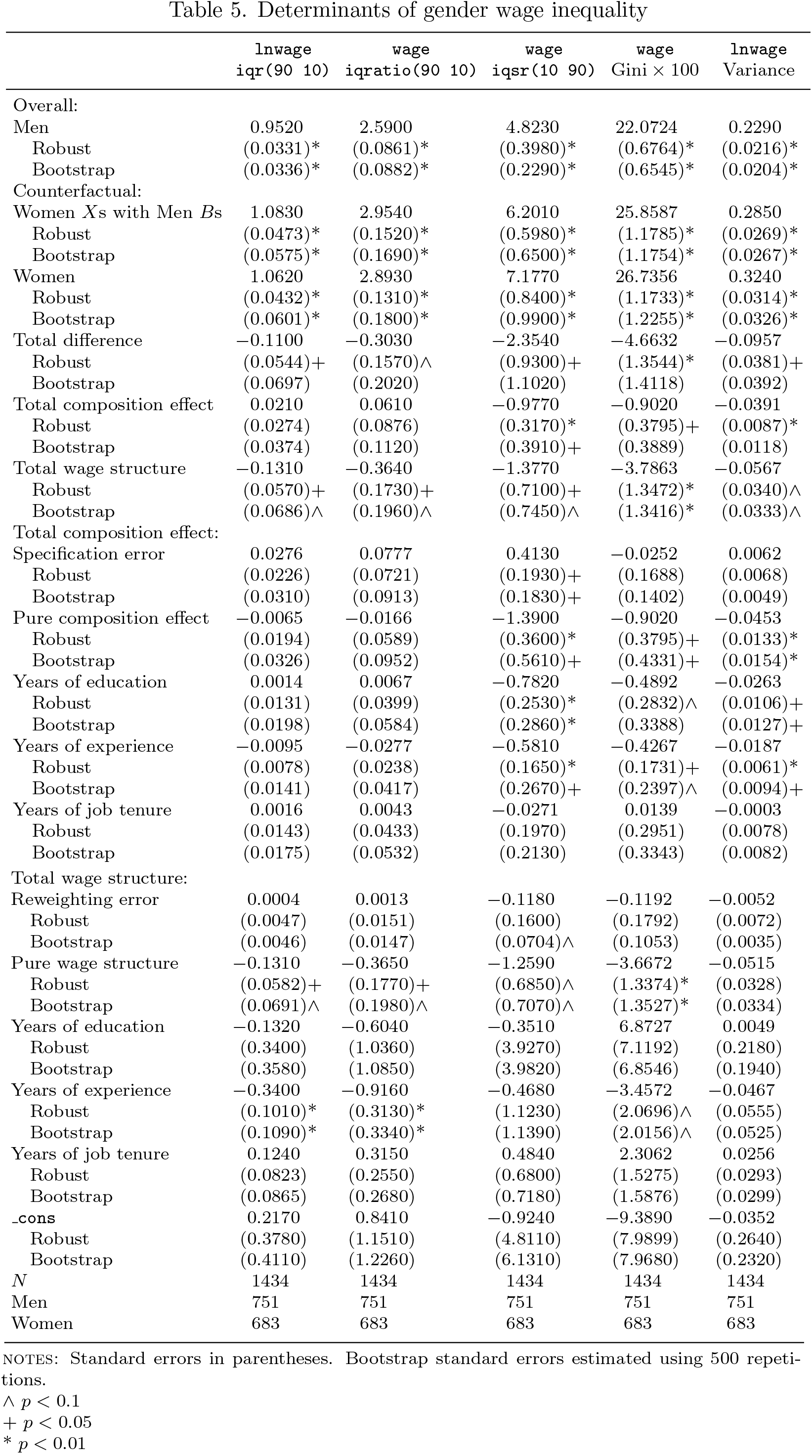
As shown for the case of RIF regressions, asymptotic and robust standard errors may not be appropriate for the decomposition of statistics related to quantiles or the Atkinson index. Furthermore, because the reweighting factors ω(X) are estimated variables, standard errors of the decomposition components need to be adjusted. Given the complexity of estimating asymptotic standard errors in the framework of RIF decompositions, the suggested alternative is to use bootstrap standard errors throughout, which can be obtained using the bootstrap prefix. Bootstrap standard errors cannot be used in combination with weights, but one can use the community-contributed command bs4rw to account for weights and survey design.

For illustration, I present in table 5 a simple exercise decomposing the same five measures of wage inequality used for the RIF regression example, analyzing differences by gender. Only results for the reweighted RIF decomposition are shown. A logit probability model is used for estimating the reweighting factors, using the same specification as the outcome model.

Table 5.

Determinants of gender wage inequality

	lnwage iqr(90 10)	wage iqratio(90 10)	wage iqsr(10 90)	wage Gini × 100	lnwage Variance
Overall:
Men	0.9520	2.5900	4.8230	22.0724	0.2290
Robust	(0.0331)*	(0.0861)*	(0.3980)*	(0.6764)*	(0.0216)*
Bootstrap	(0.0336)*	(0.0882)*	(0.2290)*	(0.6545)*	(0.0204)*
Counterfactual:
Women Xs with Men Bs	1.0830	2.9540	6.2010	25.8587	0.2850
Robust	(0.0473)*	(0.1520)*	(0.5980)*	(1.1785)*	(0.0269)*
Bootstrap	(0.0575)*	(0.1690)*	(0.6500)*	(1.1754)*	(0.0267)*
Women	1.0620	2.8930	7.1770	26.7356	0.3240
Robust	(0.0432)*	(0.1310)*	(0.8400)*	(1.1733)*	(0.0314)*
Bootstrap	(0.0601)*	(0.1800)*	(0.9900)*	(1.2255)*	(0.0326)*
Total difference	−0.1100	−0.3030	−2.3540	−4.6632	−0.0957
Robust	(0.0544)+	(0.1570)∧	(0.9300)+	(1.3544)*	(0.0381)+
Bootstrap	(0.0697)	(0.2020)	(1.1020)	(1.4118)	(0.0392)
Total composition effect	0.0210	0.0610	−0.9770	−0.9020	−0.0391
Robust	(0.0274)	(0.0876)	(0.3170)*	(0.3795)+	(0.0087)*
Bootstrap	(0.0374)	(0.1120)	(0.3910)+	(0.3889)	(0.0118)
Total wage structure	−0.1310	−0.3640	−1.3770	−3.7863	−0.0567
Robust	(0.0570)+	(0.1730)+	(0.7100)+	(1.3472)*	(0.0340)∧
Bootstrap	(0.0686)∧	(0.1960)∧	(0.7450)∧	(1.3416)*	(0.0333)∧
Total composition effect:
Specification error	0.0276	0.0777	0.4130	−0.0252	0.0062
Robust	(0.0226)	(0.0721)	(0.1930)+	(0.1688)	(0.0068)
Bootstrap	(0.0310)	(0.0913)	(0.1830)+	(0.1402)	(0.0049)
Pure composition effect	−0.0065	−0.0166	−1.3900	−0.9020	−0.0453
Robust	(0.0194)	(0.0589)	(0.3600)*	(0.3795)+	(0.0133)*
Bootstrap	(0.0326)	(0.0952)	(0.5610)+	(0.4331)+	(0.0154)*
Years of education	0.0014	0.0067	−0.7820	−0.4892	−0.0263
Robust	(0.0131)	(0.0399)	(0.2530)*	(0.2832)∧	(0.0106)+
Bootstrap	(0.0198)	(0.0584)	(0.2860)*	(0.3388)	(0.0127)+
Years of experience	−0.0095	−0.0277	−0.5810	−0.4267	−0.0187
Robust	(0.0078)	(0.0238)	(0.1650)*	(0.1731)+	(0.0061)*
Bootstrap	(0.0141)	(0.0417)	(0.2670)+	(0.2397)∧	(0.0094)+
Years of job tenure	0.0016	0.0043	−0.0271	0.0139	−0.0003
Robust	(0.0143)	(0.0433)	(0.1970)	(0.2951)	(0.0078)
Bootstrap	(0.0175)	(0.0532)	(0.2130)	(0.3343)	(0.0082)
Total wage structure:
Reweighting error	0.0004	0.0013	−0.1180	−0.1192	−0.0052
Robust	(0.0047)	(0.0151)	(0.1600)	(0.1792)	(0.0072)
Bootstrap	(0.0046)	(0.0147)	(0.0704)∧	(0.1053)	(0.0035)
Pure wage structure	−0.1310	−0.3650	−1.2590	−3.6672	−0.0515
Robust	(0.0582)+	(0.1770)+	(0.6850)∧	(1.3374)*	(0.0328)
Bootstrap	(0.0691)∧	(0.1980)∧	(0.7070)∧	(1.3527)*	(0.0334)
Years of education	−0.1320	−0.6040	−0.3510	6.8727	0.0049
Robust	(0.3400)	(1.0360)	(3.9270)	(7.1192)	(0.2180)
Bootstrap	(0.3580)	(1.0850)	(3.9820)	(6.8546)	(0.1940)
Years of experience	−0.3400	−0.9160	−0.4680	−3.4572	−0.0467
Robust	(0.1010)*	(0.3130)*	(1.1230)	(2.0696)∧	(0.0555)
Bootstrap	(0.1090)*	(0.3340)*	(1.1390)	(2.0156)∧	(0.0525)
Years of job tenure	0.1240	0.3150	0.4840	2.3062	0.0256
Robust	(0.0823)	(0.2550)	(0.6800)	(1.5275)	(0.0293)
Bootstrap	(0.0865)	(0.2680)	(0.7180)	(1.5876)	(0.0299)
cons	0.2170	0.8410	−0.9240	−9.3890	−0.0352
Robust	(0.3780)	(1.1510)	(4.8110)	(7.9899)	(0.2640)
Bootstrap	(0.4110)	(1.2260)	(6.1310)	(7.9680)	(0.2320)
N	1434	1434	1434	1434	1434
Men	751	751	751	751	751
Women	683	683	683	683	683

notes: Standard errors in parentheses. Bootstrap standard errors estimated using 500 repetitions.

∧ p < 0.1

+ p < 0.05

* p < 0.01

In general, all models suggest that inequality is higher among women compared with men. Inequality among women is between 11.5% to almost 48% higher than for men. The smallest gaps are measured for the interquartile ratio, while the largest is observed for the interquantile share ratio of wages. Controlling for differences in the distribution of years of education, tenure, and experience slightly reduces the wage inequality by almost half when looking through the wage distribution (interquantile share ratio and variance of log wages) but seems to have a marginal but increasing effect on the interquantile range and interquantile ratio.

The specification error is small but statistically significant for the interquantile share ratio model, suggesting that higher polynomials should be included to reduce the specification bias. The reweighting error suggests a good-quality reweighting because it is small and nonstatistically significant across models with the exception of the interquantile share ratio, where differences in years of experience are still important for the model.

The detailed decomposition effect suggests that women experience larger wage inequality because they have lower levels of education, experience, and job tenure (improvements in those characteristics seem to reduce wage inequality). The wage structure effect also has a negative contribution to explaining inequality because the inequalityreducing effects of education, experience, and job tenure are smaller for women compared with men.

Similarly to the results for RIF regressions, robust standard errors tend to be smaller than bootstrap standard errors, especially for statistics related to quantiles (in table 4, columns 1–3). Nevertheless, because of the two-step nature of the reweighting process, bootstrap standard errors are still recommended.

6 Conclusions

IFs and RIFs are important statistical tools that can be used to analyze the robustness of statistics to outliers and obtain asymptotic standard errors of otherwise complex distributional statistics (Cowell and Flachaire 2007; Deville 1999). Firpo, Fortin, and Lemieux (2009) expand on this literature proposing the use of RIFs in the context of regression and decomposition analysis. This is a simple strategy to analyze unconditional partial effects on any distributional statistics for which a RIF can be obtained.

This article revises the intuition behind the IF and RIF and briefly discusses the setup under which they can be used for regression and decomposition analysis. To facilitate the implementation of these strategies and make RIFs an easy-to-use tool for the applied econometrician, I introduce one function and two new commands: rifvar(), for the estimation of RIFs for a large set of distributional statistics; rifhdreg, for the estimation of RIF regressions and inequality treatment effects; and oaxaca_rif, for the estimation of standard and reweighted OB decompositions for statistics beyond the mean.

Footnotes

7 Programs and supplemental materials

To install a snapshot of the corresponding software files as they existed at the time of publication of this article, type

Notes

A Functional statistics and RIFs

This appendix provides the full set of distributional statistics, formulas, and sources.

References

Barsky

Bound

Charles

K. K.

Lupton

J. P.

2002. Accounting for the black– white wealth gap: A nonparametric approach. Journal of the American Statistical Association 97: 663–673. https://doi.org/10.1198/016214502388618401.

Blinder

A. S.

1973. Wage discrimination: Reduced form and structural estimates. Journal of Human Resources 8: 436–455. https://doi.org/10.2307/144855.

Borgen

N. T.

2016. Fixed effects in unconditional quantile regression. Stata Journal 16: 403–415. https://doi.org/10.1177/1536867X1601600208.

Cattaneo

M. D.

2010. Efficient semiparametric estimation of multi-valued treatment effects under ignorability. Journal of Econometrics 155: 138–154. https://doi.org/10.1016/j.jeconom.2009.09.023.

Cattaneo

M. D.

Drukker

D. M.

Holland

A. D.

2013. Estimation of multivalued treatment effects under conditional independence. Stata Journal 13: 407–450. https://doi.org/10.1177/1536867X1301300301.

Chung

Van Kerm

2018. Foreign workers and the wage distribution: What does the influence function reveal? Econometrics 6: 41. https://doi.org/10.3390/econometrics6030041.

Correia

2016. A feasible estimator for linear models with multi-way fixed effects. http://scorreia.com/research/hdfe.pdf.

Cowell

F. A.

Flachaire

2007. Income distribution and inequality measurement: The problem of extreme values. Journal of Econometrics 141: 1044–1072. https://doi.org/10.1016/j.jeconom.2007.01.001.

Cowell

F. A.

Flachaire

2015. Statistical methods for distributional analysis. In Handbook of Income Distribution, vol. 2, ed. Atkinson

A. B.

Bourguignon

, 359–465. The Netherlands: Elsevier.

10.

Davies

J. B.

Fortin

N. M.

Lemieux

2017. Wealth inequality: Theory, measurement and decomposition. Canadian Journal of Economics 50: 1224–1261. https://doi.org/10.1111/caje.12313.

11.

Deville

J.-C.

1999. Variance estimation for complex statistics and estimators: Linearization and residual techniques. Survey Methodology 25: 193–203.

12.

DiNardo

Fortin

N. M.

Lemieux

1996. Labor market institutions and the distribution of wages, 1973–1992: A semiparametric approach. Econometrica 64: 1001–1044. https://doi.org/10.2307/2171954.

13.

Donald

S. G.

Hsu

Y.-C.

2014. Estimation and inference for distribution functions and quantile functions in treatment effect models. Journal of Econometrics 178: 383–397. https://doi.org/10.1016/j.jeconom.2013.03.010.

14.

Efron

1982. The Jackknife, the Bootstrap and Other Resampling Plans. Philadelphia: Society for Industrial and Applied Mathematics.

15.

Essama-Nssah

Lambert

P. J.

2012. Influence functions for policy impact analysis. In Inequality, Mobility and Segregation: Essays in Honor of Jacques Silber, ed. Bishop

J. A.

Salas

, 135–159. Bingley, UK: Emerald.

16.

Firpo

Fortin

N. M.

Lemieux

2009. Unconditional quantile regressions. Econometrica 77: 953–973. https://doi.org/10.3982/ECTA6822.

17.

Firpo

Pinto

2016. Identification and estimation of distributional impacts of interventions using changes in inequality measures. Journal of Applied Econometrics 31: 457–486. https://doi.org/10.1002/jae.2448.

18.

Firpo

S. P.

Fortin

N. M.

Lemieux

2018. Decomposing wage distributions using recentered influence function regressions. Econometrics 6: 28. https://doi.org/10.3390/econometrics6020028.

19.

Fortin

Lemieux

Firpo

2011. Decomposition methods in economics. In Handbook of Labor Economics, vol. 4A, ed. Ashenfelter

Card

, 1–102. Amsterdam: Elsevier.

20.

Frölich

Melly

2010. Estimation of quantile treatment effects with Stata. Stata Journal 10: 423–457. https://doi.org/10.1177/1536867X1001000309.

21.

Hampel

F. R.

1974. The influence curve and its role in robust estimation. Journal of the American Statistical Association 69: 383–393. https://doi.org/10.2307/2285666.

22.

Heckley

Gerdtham

U.-G.

Kjellsson

2016. A general method for decomposing the causes of socioeconomic inequality in health. Journal of Health Economics 48: 89–106. https://doi.org/10.1016/j.jhealeco.2016.03.006.

23.

Jann

2008. The Blinder–Oaxaca decomposition for linear regression models. Stata Journal 8: 453–479. https://doi.org/10.1177/1536867X0800800401.

24.

Kolenikov

2010. Resampling variance estimation for complex survey data. Stata Journal 10: 165–199. https://doi.org/10.1177/1536867X1001000201.

25.

von Mises

1947. On the asymptotic distribution of differentiable statistical functions. Annals of Mathematical Statistics 18: 309–348. https://doi.org/10.1214/aoms/1177730385.

26.

Oaxaca

1973. Male–female wage differentials in urban labor markets. International Economic Review 14: 693–709. https://doi.org/10.2307/2525981.

27.

Rothe

2010. Nonparametric estimation of distributional policy effects. Journal of Econometrics 155: 56–70. https://doi.org/10.1016/j.jeconom.2009.09.001.

Recentered influence functions (RIFs) in Stata: RIF regression and RIF decomposition

Abstract

Keywords

1 Introduction

2 RIF and distributional statistics

2.1 Distributional statistics: Basics

2.2 Estimations of IFs and RIFs: Gâteaux derivative

3 Estimating RIFs: rifvar() egen function

4 RIF regression: rifhdreg

4.1 Standard RIF regression

4.2 Inequality treatment effects: Advanced options

5 RIF decomposition: oaxaca_rif

6 Conclusions

Footnotes

7 Programs and supplemental materials

Notes

A Functional statistics and RIFs

References