The random forest algorithm for statistical learning

Abstract

Random forests (Breiman, 2001, Machine Learning 45: 5–32) is a statistical- or machine-learning algorithm for prediction. In this article, we introduce a corresponding new command, rforest. We overview the random forest algorithm and illustrate its use with two examples: The first example is a classification problem that predicts whether a credit card holder will default on his or her debt. The second example is a regression problem that predicts the logscaled number of shares of online news articles. We conclude with a discussion that summarizes key points demonstrated in the examples.

1 Introduction

In recent years, the use of statistical- or machine-learning algorithms has increased in the social sciences. ¹ For instance, to predict economic recession, Liu et al. (2017) compared ordinary least-squares regression results with random forest regression results and obtained a considerably higher adjusted R-squared value with random forest regression compared with ordinary least-squares regression (Nyman and Ormerod 2017). In economics, a recent book overviews various statistical-learning algorithms for predicting economic growth and recession (Basuchoudhary, Bang, and Sen 2017). In environmental science, a recent article used learning algorithms, including least absolute shrinkage and selection operator regression, random forest, and neural networks, to predict ragweed pollen concentration based on 27 years of historical data and 85 predictor variables, with the best predictive performance obtained using random forest.

Why does random forest do better than linear regression for prediction tasks? Linear regression makes the assumption of linearity. This assumption makes the model easy to interpret but is often not flexible enough for prediction. Random decision forests easily adapt to nonlinearities found in the data and therefore tend to predict better than linear regression. More specifically, ensemble learning algorithms like random forests are well suited for medium to large datasets. When the number of independent variables is larger than the number of observations, linear regression and logistic regression algorithms will not run, because the number of parameters to be estimated exceeds the number of observations. Random forest works because not all predictor variables are used at once.

Random forest is one of the best-performing learning algorithms. For social scientists, such developments in algorithms are useful only to the extent that they can access an implementation of the algorithm. In this article, we introduce rforest, a command for random forests developed by the authors that is built on the Weka library (Witten et al. 2016; Hall et al. 2009).

The outline of this article is as follows: In section 2, we briefly discuss the random forest algorithm. In section 3, we give the syntax of the rforest command. In section 4, we give an example for predicting whether a given credit card user will default on his or her debt. In section 5, we give an example for estimating the log-scaled number of shares of online news articles. In section 6, we conclude with a discussion.

2 The random forest algorithm

We first discuss tree-based models because they form the building blocks of the random forest algorithm. A tree-based model involves recursively partitioning the given dataset into two groups based on a certain criterion until a predetermined stopping condition is met. At the bottom of decision trees are so-called leaf nodes or leaves.

Figure 1 illustrates a recursive partitioning of a two-dimensional input space with axis-aligned boundaries—that is, each time the input space is partitioned in a direction parallel to one of the axes. Here the first split occurred on x ₂ ≥ a ₂. Then, the two subspaces were again partitioned: The left branch was split on x ₁ ≥ a ₄. The right branch was first split on x ₁ ≥ a ₁, and one of its subbranches was split on x ₂ > a ₃. Figure 2 is a graphical representation of the subspaces partitioned in figure 1.

Figure 1.

Recursive binary partition of a two-dimensional subspaces

Figure 2.

A graphical representation of the decision tree in figure 1

Depending on how the partition and stopping criteria are set, decision trees can be designed for both classification tasks (categorical outcome, for example, logistic regression) and regression tasks (continuous outcome).

For both classification and regression problems, the subset of predictor variables selected to split an internal node depends on predetermined splitting criteria that are formulated as an optimization problem. A common splitting criterion in classification problems is entropy, which is the practical application of Shannon’s (2001) source coding theorem that specifies the lower bound on the length of a random variable’s bit representation. At each internal node of the decision tree, entropy is given by the formula

$E=-{\displaystyle \sum _{i=1}^c{p}_i\hspace{0.17em}\times \hspace{0.17em}\log \left(p_i\right)}$

where c is the number of unique classes and p_i is the prior probability of each given class. This value is maximized to gain the most information at every split of the decision tree. For regression problems, a commonly used splitting criterion is the mean squared error at each internal node.

A drawback of decision trees is that they are prone to overfitting, which means that the model follows the idiosyncrasies of the test dataset too closely and performs poorly on a new dataset—that is, the test data. Overfitting decision trees will lead to low general predictive accuracy, also referred to as generalization accuracy.

One way to increase generalization accuracy is to consider only a subset of the observations and build many individual trees. First introduced by Ho (1995), this idea of the random-subspace method was later extended and formally presented as the random forest by Breiman (2001). The random forest model is an ensemble tree-based learning algorithm; that is, the algorithm averages predictions over many individual trees. The individual trees are built on bootstrap samples rather than on the original sample. This is called bootstrap aggregating or simply bagging, and it reduces overfitting. The algorithm is as follows:

Algorithm 1.

Random forest algorithm

Individual decision trees are easily interpretable, but this interpretability is lost in random forests because many decision trees are aggregated. However, in exchange, random forests often perform much better on prediction tasks.

The random forest algorithm more accurately estimates the error rate compared with decision trees. More specifically, the error rate has been mathematically proven to always converge as the number of trees increases (Breiman 2001).

The error of the random forest is approximated by the out-of-bag (oob) error during the training process. Each tree is built on a different bootstrap sample. Each bootstrap sample randomly leaves out about one-third of the observations. These left-out observations for a given tree are referred to as the oob sample. Finding parameters that would produce a low oob error is often a key consideration in model selection and parameter tuning. Note that in the random forest algorithm, the size of the subset of predictor variables, m, is crucial to controlling the final depth of the trees. Hence, it is a parameter that needs to be tuned during model selection, which will be discussed in the examples later.

To gain some insight on the complex model, we calculate the so-called variable importance of each variable. This is calculated by adding up the improvement in the objective function given in the splitting criterion over all internal nodes of a tree and across all trees in the forest, separately for each predictor variable. In the Stata implementation of random forest, the variable importance score is normalized by dividing all scores over the maximum score: the importance of the most important variable is always 100%.

3 Syntax

The syntax to fit a random forest model is

rforest depvar indepvars [if] [in] [, type( string ) iterations( int )

numvars( int )depth( int ) lsize( int ) variance( real ) seed( int )

numdecimalplaces( int )]

with the following postestimation command:

predict newvar | varlist | stub * [if] [in] [, pr]

4 Example: Credit card default

Yeh and Lien (2009) and Dheeru and Karra Taniskidou (2017) investigated the predictive accuracy of the probability of default of credit card clients. There are a total of 30,000 observations, 1 response variable, 22 explanatory variables, and no missing values. The response variable is a binary variable that encodes whether the card holder will default on his or her debt, with 0 encoded as “no default” and 1 encoded as “default”. Of the 22 explanatory variables, 10 are categorical variables containing information such as gender, education, marital status, and whether past payments have been made on time or delayed. The remaining 12 continuous explanatory variables contain information on the monthly bill amount and payment amount over 6 months. For a complete list of variables, please refer to appendix A.

In this example, we will investigate the predominant factors that affect credit card default prediction accuracy, and we will contrast the prediction accuracies obtained using random forest and logistic regression.

4.1 Model training and parameter tuning

To start the model-training process, we arrange the data points in a randomly sorted order. When the data are split into training and test data, a random sort order ensures that the training data are random as well. To allow for reproducible results, we set a seed value. Then, we split the dataset into two subsets: 50% of the data are used for training, and 50% of the data are used for testing (validation). In small datasets, a 50-50 split may reduce the size of the training data too much; for this relatively large dataset, a 50-50 split is not problematic. The randomization process mentioned previously ensures that the training data contain observations belonging to all available classes as long as the class probabilities are not heavily imbalanced. Additionally, it removes the model’s potential dependency on the ordering of observations relative to the test data. Finally, because the variable for marital status uses values 0, 1, 2, and 3 to encode unordered categorical information, we need to create four new binary indicator variables for each marital status using the command tabulate marriage, generate(marriage_enum). Creating the fourth indicator variable is redundant, but this does not matter to tree-based algorithms like rforest.

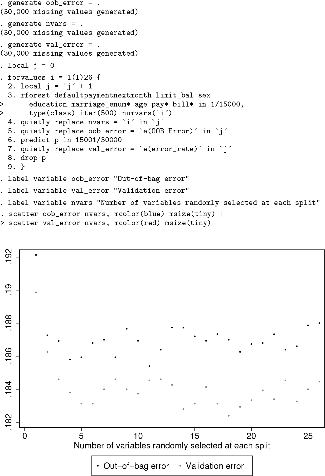
Next, we tune the hyperparameters to find the model with the highest testing accuracy. Specifically, we tune the number of iterations (that is, the number of subtrees) and number of variables to randomly investigate at each split, numvars(). The following code segment iteratively calculates the oob prediction accuracy as a function of the number of iterations and numvars(). The number of iterations starts at 10 and is incremented by 5 every time until it reaches 500. We will use both a oob error (tested against training data subsets that are not included in subtree construction) and a validation error (tested against the testing data) to determine the best possible model.

Usually, tuning parameters in statistical-learning models requires a grid search, that is, an exhaustive search on a user-specified subspace of hyperparameter values. In this case, however, because random forest oob error rates converge after the number of iterations gets large enough, we simply need to set the iterations to a value large enough for convergence to have occurred prior to tuning the numvars() parameter.

To illustrate how the oob error and validation error have similar trends as the number of iterations grow, we call the random forest function iteratively. The number of iterations variable is initialized to 10 and increments by 5 per function call until it reaches 500. Finally, the trends of oob error and validation error can be visualized by plotting those values against the number of iterations, as shown in figure 3.

The stable option ensures that the result replicates even if there are ties on the sort variable. The number of variables is investigated below; for simplicity, we set numvars(1) here.

Figure 3.

oob error and validation error versus iterations plot

We can see from figure 3, generated by the above code block, that both the oob error and the validation error stabilize at around 19%. Hence, fixing the number of iterations at 500 is a good choice.

Next, we can tune the hyperparameter numvars():

Figure 4.

oob error and validation error versus number of variables plot

In figure 4, we can see for how many variables the minimum error occurs. The following code automates finding the minimum error and the corresponding number of variables. (This code uses frames and requires Stata 16.)

We can see that at numvars(18), we get the lowest validation error at 0.1824. Hence, we will use numvars(18) for our final model.

In principle, the random forest algorithm can output an oob error at each iteration. However, the Weka implementation of random forest used for the Stata plugin does not output running calculations of oob error as the algorithm runs and instead only outputs one final oob error for the total number of iterations. This means that tuning the iterations parameter requires running the random forest algorithm k times for every value of iterations( k ). To make this process efficient, we set minimum and maximum values and a reasonable increment to see the trend of the change of oob error over increasing iterations.

4.2 Final model and interpretation of results

As shown in the previous section, we have set the values of the hyperparameters to be iterations(500) and numvars(18). Having reached convergence after 500 iterations, we are free to set the number of iterations even higher. Out of an abundance of caution we set iterations(1000). The following code block gives the final model and prediction error:

The final oob error is 18.25%, which is larger than the actual prediction error, which is 18.24%, calculated over 15,000 test observations. We can see from both figure 3 and figure 4 that the oob error and the validation error have the same pattern when plotted against the two hyperparameters, which are iterations and number of variables.

We also would like to ascertain which factors are the most important in the prediction process. Random forests are black boxes in that they do not offer insight on how the predictions are accomplished. The variable-importance scores of each predictor provide some limited insight. The following code segment plots the variable importance:

We can see from figure 5 that the five most important predictors are basic demographic and background information such as gender, education, and marital status (“married” and “single”) as well as the monthly spending limit (limit_bal). We can also see that none of the variables encoding monthly bill amounts (bill_amt) is particularly important, compared with the rest of the predictors. Surprisingly, however, the amount of monthly spending limit (limit_bal) is the third most important predictor in the random forest model. We can overlay two histograms of the monthly spending limit to obtain more insight on how this variable affects the response variable:

Figure 5.

Importance scores of predictor variables

We can see from the histograms in figure 6 that card holders who default on their debt generally have a lower monthly spending limit than those who do not default. Variable importance measures the contribution of an x variable to the model but depends on the set of x variables. Another x variable correlated with the first would rise in importance if the first x variable was excluded.

Figure 6.

Histograms of monthly spending limit

4.3 Comparison with logistic regression

Alternatively, credit card debt default can be modeled using logistic regression. The following code returns the prediction accuracy of logistic regression using the same set of predictor variables and the same train-and-test split:

The prediction error obtained using logistic regression is 18.86%, compared with the best-so-far error rate that we have from random forest, which is 18.25%. The difference in error rate is small but might still be meaningful to prevent credit card defaults.

5 Example: Online news popularity

Fernandes et al. (2015) and Dheeru and Karra Taniskidou (2017) investigated the popularity of online news. ² The data were originally presented at a Portuguese conference on artificial intelligence in 2015. There are a total of 39,644 observations, 1 response variable, and 58 explanatory variables. For this problem, we are interested in the log-scaled number of “shares” an online article obtains based on various nominal and continuous attributes such as whether the article was published on a weekend, whether certain keywords are present, number of images in the article, etc. For a full list of variable names and descriptions, please refer to appendix B.

5.1 Model training and parameter tuning

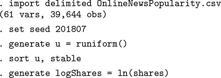
First, we need to randomize the data as we did for the previous classification example. Then, we generate a new variable for the log-scaled number of shares:

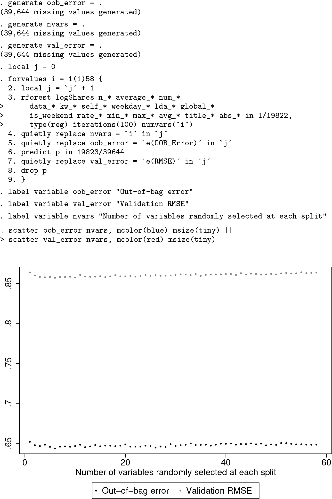
We will use a 50-50 split to partition the data into training and testing sets as in the previous example. To tune the hyperparameters numvars() and iterations(), we use the same technique as the previous example, where we fix the value of one hyperparameter when tuning the other. This is a viable parameter-optimization method that results from the error rate for random forest converging when the number of iterations is large enough. Essentially, our goal is to set a reasonably large number of iterations where the oob and validation errors converge so that when we tune the number of randomly selected variables, we can ascertain that the errors differ because of the value of numvars() and not because of iterations(). We will again start with iterations(10) and increase it by increments of 5 until iterations(100), which is approximately the highest possible value with which one can run this dataset on a CPU because of constraints on runtime memory. At the end of the loop, we plot the oob errors and the actual root mean squared error (rmse) values validated using the test data against the number of iterations.

Figure 7.

oob error and validation rmse versus iterations plot

We can see from the graph that the oob error and validation rmse start to converge around 80 iterations. We get the lowest value for both errors at 100 iterations, which will be used for the final model. Now we can tune the other hyperparameter, numvars(), to see which one gives the lowest validation rmse.

Figure 8.

oob error and validation error versus number of variables plot

Again, we automate finding the minimum error:

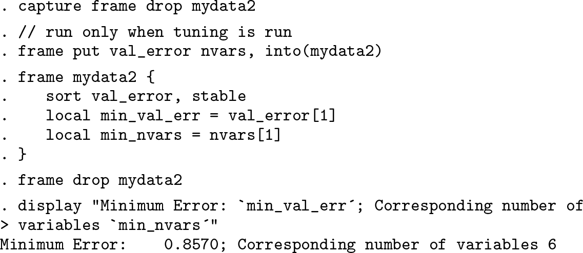
For numvars(6), we get the lowest validation error at 0.8570. Hence, we will use numvars(6) for our final model. For this dataset, the model is fairly robust to changes in the number of variables, numvars(), and numvars(6) has only a slight edge compared with other values. This might not always be the case.

5.2 Final model and interpretation of results

The final model has hyperparameter values numvars(6) and iterations(100).

The final oob error is 0.6436. This is slightly lower than the rmse calculated against the testing data, which is 0.8570. To learn which variables affect the prediction accuracy, we can generate a variable-importance plot using the same code segment as the previous classification example. For readability, only variables with an importance score of at least 40% as large as that of the most important variable are shown.

Figure 9.

Importance score of predictor variables

Whether the article was published on a weekend is the most important predictor. Other important explanatory variables include news channel types and the number of keywords. To obtain more insight on how the log-scaled number of article shares is related to whether the article was published on a weekend, we use the following histogram to illustrate the relationship:

Figure 10.

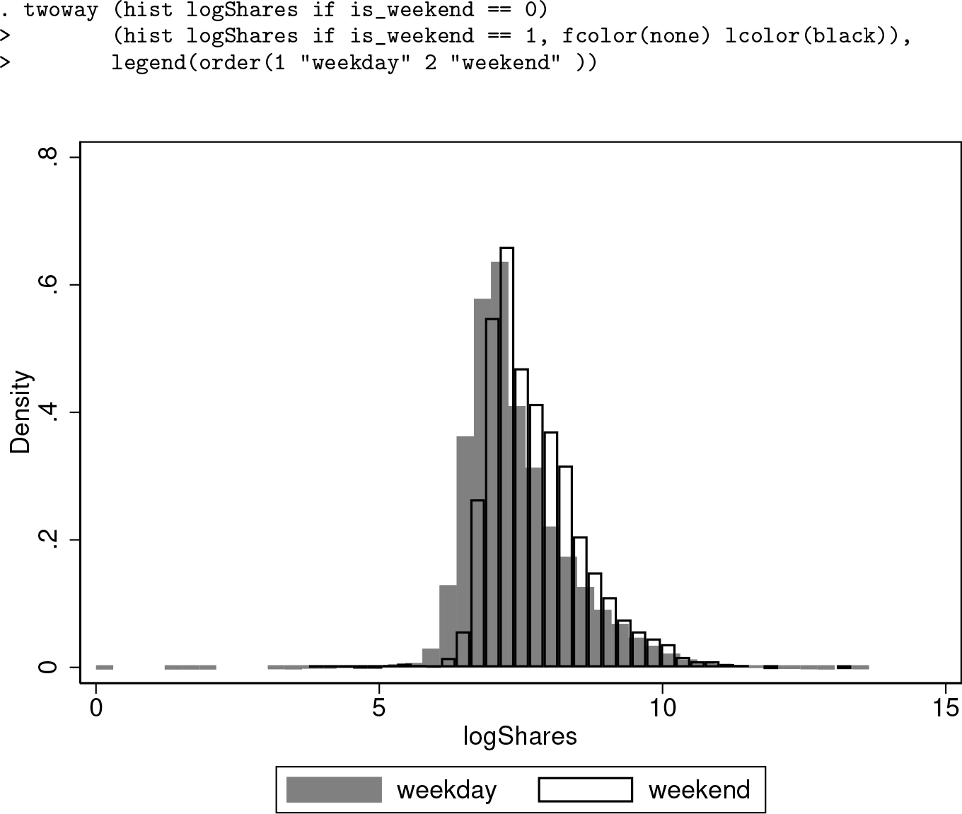
Histograms of log-scaled number of shares

The empirical distributions of log number of shares differ for weekdays versus weekends. This clear shift in empirical distribution helps to explain why the is_weekend explanatory variable was the most important in the model.

5.3 Comparison with linear regression

The following code block fits a linear regression model over the same set of dependent and independent variables using the same train-and-test split as shown in the random forest model:

The value of e(rmse) displayed is the rmse calculated over the training data. To compare the linear model with the random forest model, we need to calculate the rmse over the testing data using the following commands:

We can see from the output that the mean squared error is 40.90379, which means the rmse is equal to $\sqrt{40.90379}\approx 6.3956$ , which is much higher than the rmse fitted over the training data. Comparing with the testing rmse obtained from the random forest model, the testing rmse for the linear model is much higher. This is a strong indication that random forest outperforms linear regression for this example.

6 Discussion

The classification and regression examples have illustrated that random forest models usually have higher prediction accuracy than corresponding parametric models such as logistic regression and linear regression. Typically, greater gains in model performance are available for multiclass (multinomial) outcomes and regression than binary outcomes. Misclassification is a fairly insensitive performance criterion. When an improved algorithm changes the estimated classification probabilities for two classes from p ₁ = 0.10 and p ₂ = 0.90 to p ₁ = 0.40 and p ₂ = 0.60 for an observation, the resulting classification remains the same. An improvement over logistic regression with its linearity assumption can come either from nonlinearities or from interactions. Additionally, the scope of improvement is reduced when many of the variables are indicator variables; nonlinearities do not exist for indicator variables. In our experience, many of the variables in social sciences are indicator variables. For example, Ing et al. (2019) found that support-vector machines did not improve over logistic regression. Similarly, in our classification example, the improvement of random forest over logistic regression was minor.

In the examples, the values of hyperparameters were determined based on which value gave the lowest testing error. In practice, when there are not enough observations to allow for a train-and-test split, the oob error can be used instead. As previously demonstrated, the oob error is a close estimation of the actual testing error and can be used on its own as a criterion for parameter tuning.

While the two examples primarily focused on the typical case of tuning the options iterations() and numvars(), depending on the dataset and software constraints, other hyperparameters such as max tree depth and minimum size of leaf nodes could be taken into consideration during parameter tuning. For instance, setting the max tree depth to a fixed value may become necessary on a machine with limited RAM.