Many instruments: Implementation in Stata

Abstract

In recent decades, econometric tools for handling instrumental-variable regressions characterized by many instruments have been developed. We introduce a command, mivreg, that implements consistent estimation and testing in linear instrumental-variables regressions with many (possibly weak) instruments. mivreg covers both homoskedastic and heteroskedastic environments, estimators that are both nonrobust and robust to error nonnormality and projection matrix limit, and parameter tests and specification tests both with and without correction for existence of moments. We also run a small simulation experiment using mivreg and illustrate how mivreg works with real data.

1 Introduction

Instrumental-variables (IV) estimation and inference have long been a distinctive method in applied microeconometric analysis and have often spurred advances in econometric theory. The IV methods were designed to address endogeneity bias from ordinary least squares (OLS) in fitting a causal or treatment effect in structural models (such as an effect of smoking on health, returns to education, or demand elasticity); see Angrist and Krueger (2001). At the dawn of the 21st century, both theory and practice were extended to accommodate such complications as weak instruments, numerous instruments, and combinations thereof. It was established that the empiricist’s workhorse, the two-stage least-squares (2SLS) estimator, fails to deliver consistent estimates and results in invalid inference when such complications arise, and alternative approaches to estimation and inference were proposed. However, the quick progress in econometric theory did not carry over to empirical practice as quickly.

The seminal article by Bekker (1994) proposed an alternative asymptotic approximation for linear normal homoskedastic IV regressions with many IV together with consistent estimation and construction of valid standard errors within the new paradigm of dimension asymptotics. Since then, there has been significant progress in the theory of estimation and testing in IV regressions with many (possibly weak) instruments. Many new or modified versions of old estimators and tests have been proposed, including limited-information maximum-likelihood (LIML), bias-corrected 2SLS, several versions of jackknife IV estimators, etc. Hansen, Hausman, and Newey (2008) proposed extensions of estimation and inference methods based on LIML, particularly when the structural and first-stage errors are not necessarily normal and when the instruments may be weak as a group. More recently, Hausman et al. (2012) showed that the leading “homoskedastic” estimators fail to deliver consistency in heteroskedastic models and proposed their “heteroskedastic” modifications. Anatolyev and Gospodinov (2011) and Lee and Okui (2012) developed specification testing tools for the homoskedastic case, and Chao et al. (2014) developed specification testing tools for the heteroskedastic case.

The state-of-the-art theoretical literature has converged to suggesting estimation based on LIML and its Fuller (1977)-type correction that remedies the problem of nonexistence of moments. Parameter inference is based on consistent estimation of up to four terms in the asymptotic variance, while specification testing is based on asymptotically normal (or asymptotically equivalent possibly adjusted chi-squared) distribution of the overidentifying test statistic. The literature has shown that all of these tools are robust to weakness of the instruments as a group (though weakness of a lesser degree than that would jeopardize identification). We briefly describe these tools in the following sections; see Anatolyev (2019) for more technical details and the history of theoretical developments and suggestions of empirical strategies.

Despite the theoretical advances, practitioners rarely use appropriate tools because of their nonavailability in popular econometric packages, Stata in particular. This article aims to fill this void. We introduce a command, mivreg, that implements consistent estimation and testing in linear IV regressions with many (possibly weak) instruments. mivreg covers both homoskedastic and heteroskedastic environments, estimators that are both nonrobust and robust to error nonnormality and projection matrix limit, and both parameter and specification tests. Even though, as noted above, other consistent estimators have been proposed, we build up mivreg around the leading LIML estimator and its Fuller (1977) correction as suggested by the state-of-the-art literature.

In section 2, we set out the model and introduce necessary notation. In sections 3 and 4, we describe estimation and testing tools pertaining to the homoskedastic and heteroskedastic models, respectively. In section 5, we present the new command, mivreg. In section 6, we illustrate how mivreg works in simulations and compare it with the classical command ivregress. Finally, in section 7, we illustrate how mivreg works with real data.

2 Model

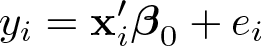
The structural equation is

$y_{\text{i}}=x_i^{{ }^{\prime }}{\beta }_0+e_{\text{i}}$

where β ₀ is a k × 1 vector of structural coefficients of interest, or in matrix notation, $Y=X{\beta }_0+e$ , where $Y=(y_{\text{1}}, . . . , y_{\text{n}})\prime$ is n × 1, $X=(x_{\text{1}}, . . . ,x_{\text{n}})\prime$ is n × k, and $e=(e_{\text{1}}, . . . , e_{\text{n}})\prime$ is n × 1. The first-stage equation is

$x_{\text{i}}=z_i^{\prime }\Gamma +u_{\text{i}}$

where z _i is an ℓ×1 vector of instruments and Γ is an ℓ×k matrix of first-stage coefficients, or in matrix notation, $X=Z\Gamma +U$ , where $U=(u_{\text{1}}, . . . ,u_{\text{n}})\prime$ is n × k. We assume that the rank of instrument matrix $Z=(z_{\text{1}}, . . . ,z_{\text{n}})\prime$ equals its column dimension ℓ. The structural and first-stage errors follow

$\left(\begin{array}{c}{e}_i\\ u_i\end{array}\right)|z\text{i}~D\left(\left(\begin{array}{c}0\\ 0\end{array}\right),\left(\begin{array}{cc}{\sigma }_i^2& {\Psi }_i^{\prime }\\ {\Psi }_i& {\Omega }_i\end{array}\right)\right)$

for some distribution D, with normal N being a possibility. Under conditional homoskedasticity, ${\sigma }_i^2={\sigma }^{\text{2}},{\Psi }_{\text{i}}=\Psi$ and ${\Omega }_{\text{i}}=\Omega$ for all $i=\text{ 1}, . . . , n$ .

Introduce the projection matrices associated with the instruments

$P=Z{(Z^{\prime }Z)}^{-\text{1}}{Z}^{\prime },M=I_{\text{n}}-P$

The (i, j)th element of P is denoted P _ij. Let us also denote by D the diagonal matrix with diagonal elements of P on the main diagonal: $D=\text{ diag}{\left\{P_{\text{ii}}\right\}}_i^n=\text{1}$ . We denote by $\overline{P_{ii}^2}$ an average of diagonal elements of P squared: $\overline{P_{ii}^2}=n^{-\text{1}}\text{tr}\left(D^{\text{2}}\right)$ .

3 Homoskedastic case

In the conditionally homoskedastic case, Bekker (1994) and Hansen, Hausman, and Newey (2008) developed correct parameter estimation and inference. Anatolyev and Gospodinov (2011) and Lee and Okui (2012) dealt with specification testing.

3.1 Point estimation

Under many instruments, 2SLS estimation is inconsistent. The leading consistent estimator is the LIML estimator

${\widehat{\beta }}_{\text{LIML}}=\begin{array}{c}\text{arg min}\\ \beta \end{array}\frac{(Y-X\beta )\prime P(Y-X\beta )}{(Y-X\beta )\prime (Y-X\beta )}$

Numerically, instead of the above optimization problem, it can be found via the eigenvalue problem

${\widehat{\beta }}_{\text{LIML}}={\overline{H}}^{-}{ }^{\text{1}}X\prime \stackrel{\circ }{P}Y$

where

$\overline{H}=X\prime \stackrel{\circ }{P}X$

and $\stackrel{\circ }{P}=P-\overline{\alpha }{I}_{\text{n}}$ , and $\overline{\alpha }$ is the smallest eigenvalue of the matrix ${\left(\begin{array}{cc}\stackrel{\circ }{X^{\prime }}& \stackrel{\circ }{X}\end{array}\right)}^{-\text{1}}\stackrel{\circ }{X^{\prime }}P\stackrel{\circ }{X}$ , where $\stackrel{\circ }{X} =(Y,X).$

The LIML estimator has a disadvantage that even its low-order moments do not exist. A simple Fuller (1977) adjustment solves the moment problem:

$\tilde{\alpha }=\frac{\overline{\alpha }-\left(1-\overline{\alpha }\right)\varsigma /n\hspace{0.17em}}{1-\left(1-\overline{\alpha }\right)\varsigma /n}$

1

This adjustment leads to the FULL estimator, where $\overline{\alpha }$ is replaced by αe everywhere. It is usually advised to use the value ς = 1 in practice.

Denote the vector of LIML or FULL residuals by $\widehat{e}$ , then

${\widehat{\sigma }}^{\text{2}}=\frac{\widehat{e}\prime \widehat{e}}{n-k}$

is the residual variance.

3.2 Variance estimation

Under error normality or an asymptotically constant diagonal of P, the asymptotic variance is estimated by

$\overline{V}=n{\overline{H}}^{-\text{1}}{\overline{\Sigma }}_0{\overline{H}}^{-\text{1}}$

where

${\overline{\Sigma }}_0={\widehat{\sigma }}^{\text{2}}\left\{{(\text{1}-\overline{\alpha })}^{\text{2}}\overline{X}\prime P\overline{X}+{\overline{\alpha }}^{\text{2}}\overline{X}\prime (I_{\text{n}}-P)\overline{X}\right\}$

and

$\overline{X}=X-\widehat{e}\frac{\widehat{e}\prime X}{\widehat{e}\prime \widehat{e}}$

(Bekker 1994; Hansen, Hausman, and Newey be′be 2008).

Under error nonnormality and an asymptotically variable diagonal of P, the asymptotic variance is estimated by

${\overline{V}}_{\text{R}}=n{\overline{H}}^{-\text{1}}\left({\overline{\Sigma }}_0+{\overline{\Sigma }}_{\text{A}}+\overline{\Sigma }{\prime }_{\text{A}}+{\overline{\Sigma }}_{\text{B}}\right){\overline{H}}^{-\text{1}}$

where the subscript R stands for “robust”. Additionally,

${\overline{\Sigma }}_{\text{A}}=\left\{{\displaystyle \sum _{i=1}^n\left(P_{ii}-\frac{\mathcal{l}}{n}\right)}{(PX)}_i\right\}{\left\{\frac{1}{n}{\displaystyle \sum _{i=1}^n{\widehat{e}}_i^2}{\left(M\overline{X}\right)}_i\right\}}^{\prime }$

and

${\overline{\Sigma }}_B=\frac{\overline{P_{ii}^2}-{\left(\mathcal{l}/n\right)}^2}{1-2\mathcal{l}/n+\overline{P_{ii}^2}}{\displaystyle \sum _{i=1}^n\left({\widehat{e}}_i^2-{\widehat{\sigma }}^2\right)}{\left(\text{M}\overline{X}\right)}_i{\left(\text{M}\overline{X}\right)}_i^{{ }^{\prime }}$

(Hansen, Hausman, and Newey 2008).

The variance estimates $\overline{V}$ and ${\overline{V}}_{\text{R}}$ are a basis of parameter inference. For example, the standard error for the jth parameter can be computed as $\sqrt{{\overline{V}}_{jj}/n}$ .

3.3 Specification testing

Consider the conventional J statistic

$J=\frac{\widehat{e}\prime P\widehat{e}}{{\widehat{\sigma }}^{\text{2}}}=(n-k)\overline{\alpha }$

and the bias-corrected J statistic

$J_{\text{R}}=J-\frac{\mathcal{l}}{n}\frac{\widehat{e}\prime \widehat{e}}{{\widehat{\sigma }}^{\text{2}}}=(n-k)\left(\overline{\alpha }\text{}-\frac{\mathcal{l}}{n}\right)$

where the subscript R stands for “robust”.

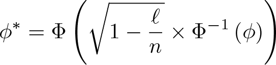
Under error normality or an asymptotically constant diagonal of P, the Anatolyev and Gospodinov (2011) test prescribes rejecting correct model specification at significance level ϕ when the value of J exceeds $q_{\varphi *}^{{\chi }^2(\mathcal{l}-\text{k})}$ , the $(\text{1}-{\varphi }^{*})$ -quantile of the chisquared with ℓ − k degrees of freedom, where

${\varphi }^{*}=\Phi \left(\sqrt{\text{1}-\frac{\mathcal{l}}{n}}\times {\Phi }^{-}{ }^{\text{1}}\left(\varphi \right)\right)$

Under error nonnormality and an asymptotically variable diagonal of P, the Lee and Okui (2012) test prescribes rejecting correct model specification at significance level ϕ when the value of

$\frac{J_{\text{R}}}{\sqrt{n{\widehat{V}}^{\text{J}}}}$

exceeds $q_{\varphi }^{N(0,\text{1})}$ , the (1 − ϕ)-quantile of the standard normal. Here

${\widehat{V}}^{\text{J}}=\text{ 2}\frac{\mathcal{l}}{n}\left(1-\frac{\mathcal{l}}{n}\right)+\left\{\overline{P_{ii}^2}-{\left(\frac{\mathcal{l}}{n}\right)}^2\right\}\left(\frac{\overline{{\widehat{e}}_i^4}}{{\widehat{\sigma }}^4}-3\right)$

4 Heteroskedastic case

In the conditionally heteroskedastic case, correct parameter estimation and inference were developed in Hausman et al. (2012). Specification testing was dealt with in Chao et al. (2014).

4.1 Point estimation

The heteroskedastic limited-information maximum-likelihood (HLIM) estimator is

${\widehat{\beta }}_{\text{HLIM}}=\begin{array}{c}\text{arg min}\\ \beta \end{array}\frac{{\left(Y-X\beta \right)}^{\prime }(P-D) (Y-X\beta )}{{(Y-X\beta )}^{\prime }(Y-X\beta )}$

Numerically, it can be found via the eigenvalue problem,

${\widehat{\beta }}_{\text{HLIM}}={\overline{H}}^{-}{ }^{\text{1}}{X}^{\prime }\stackrel{\circ }{P}Y$

where

$\overline{H}=X^{\prime }\stackrel{\circ }{P}X$

and $\stackrel{\circ }{P} =P-D-\overline{\alpha }{I}_{\text{n}}$ , and $\overline{\alpha }$ is the smallest eigenvalue of the matrix ${(\stackrel{\circ }{X^{\prime }}\stackrel{\circ }{X})}^{-\text{1}}\stackrel{\circ }{X^{\prime }}(P-D)\stackrel{\circ }{X}$ , where $\stackrel{\circ }{X}=(Y,X)$ . Similarly to FULL, the Fuller (1977) adjustment (1) leads to heteroskedastic FULL (HFUL) estimation.

Denote the vector of HLIM or HFUL residuals by $\widehat{e}$ , then

${\widehat{\sigma }}^{\text{2}}=\frac{\widehat{e}\prime \widehat{e}}{n-k}$

is the residual variance.

4.2 Asymptotic variance estimation

Hausman et al. (2012) provide a valid and robust variance estimator for the HLIM estimator,

$\overline{V}=n{\overline{H}}^{-\text{1}}{\overline{\Sigma H}}^{-\text{1}}$

where

$\overline{\Sigma }={\displaystyle \sum _{i=1}^n\left\{{\left(P\overline{X}\right)}_i{\left(P\overline{X}\right)}_i^{{ }^{\prime }}-P_{ii}{\overline{X}}_i{\left(P\overline{X}\right)}_i^{\prime }-{\left(P\overline{X}\right)}_i{\overline{X}}_i^{\prime }\right\}}{\widehat{e}}_i^2+{\displaystyle \sum _{i=1}^n{\displaystyle \sum _{j=1}^n{p}_{ij}^2}}{\overline{X}}_i{X}^{\prime }{ }_j{\widehat{e}}_i\widehat{e}\widehat{j}$

2

where

$\overline{X}=X-\widehat{e}\frac{\widehat{e}\prime X}{\widehat{e}\prime \widehat{e}}$

The variance estimate $\overline{V}$ is a basis of be′be parameter inference. For example, the standard error for the jth parameter can be computed as $\sqrt{{\overline{V}}_{jj}/n}$ .

4.3 Specification testing

Chao et al. (2014) generalize the specification J test for the heteroskedastic case. Their statistic is based on the jackknife modification of the J statistic’s quadratic form,

$J=\widehat{e}\prime \frac{(P-D)\widehat{e}}{\sqrt{{\widehat{V}}^J}}+\mathcal{l}$

where

${\widehat{V}}^{\text{J}}=\frac{1}{\mathcal{l}}{\displaystyle \sum _{i\ne j}{\widehat{e}}_i^2}{P}_{ij}^2{\widehat{e}}_i^2=\frac{1}{\mathcal{l}}\left({\displaystyle \sum _{i=1}^n{\displaystyle \sum _{j=1}^n{\widehat{e}}_i^2{P}_{ij}^2{\widehat{e}}_j^2}}-{\displaystyle \sum _{i=1}^n{P}_{ij}^2{\widehat{e}}_j^4}\right)$

3

is an estimate of the variance of the modified quadratic form.

The test is one sided, and the decision rule is to reject the null of instrument validity if the value of J exceeds $q_{\varphi }^{{\chi }^2}(\mathcal{l}-\text{k})$ , the (1 − ϕ)-quantile of the ${\chi }^{\text{2}}(\mathcal{l}-k)$ distribution.

5 The mivreg command

5.1 Functionality

The command mivreg implements estimation, inference on individual parameters and specification testing under many (possibly weak) instruments. The default hom (for “homoskedastic”) option is based on the LIML or FULL estimators; the het (for “heteroskedastic”) option is based on the HLIM or HFUL estimators. Within the hom version, the robust option leads to the Hansen–Hausman–Newey variance estimator and Lee–Okui specification test, while the default nonrobust variation computes the Bekker variance estimator and Anatolyev–Gospodinov specification test. The “hetero” version implements the Hausman–Newey–Woutersen–Chao–Swanson variance estimator and Chao–Hausman–Newey–Swanson–Woutersen specification test. By default, the estimators used are LIML or HLIM; the fuller option makes the Fuller correction with parameter ς = 1, so the FULL or HFUL estimators are used instead.

5.2 Syntax

mivreg depvar [ indepvars ] ( varlist1 = varlist2 ) [ if ] [ in ] [, hom het robust fuller level( # )]

by, rolling, statsby, and xi are allowed; see [U] 11.1.10 Prefix commands.

5.3 Description

The command mivreg performs estimation, inference on individual parameters, and specification testing under many (possibly weak) instruments. The dependent variable depvar is modeled as a linear function of indepvars and varlist1, using varlist2 (along with indepvars) as instruments for varlist1.

5.4 Options

hom uses the LIML (default) or FULL (in combination with the fuller option) estimator.

het uses the HLIM (default) or HFUL (in combination with the fuller option) estimator.

robust leads, under the hom option, to the Hansen–Hausman–Newey variance estimator and the Lee–Okui specification test, while the default nonrobust variation computes the Bekker variance estimator and the Anatolyev–Gospodinov specification test. Under the het option, robust leads to the Hausman–Newey–Woutersen–Chao–Swanson variance estimator and the Chao–Hausman–Newey–Swanson–Woutersen specification test.

fuller makes the Fuller correction with parameter ς = 1, which leads to the FULL (in combination with the hom option) or HFUL (in combination with the het option) estimator.

level(#) sets the confidence level. The default is level(95).

5.5 Stored results

mivreg stores the following in e():

5.6 Computational notes

First, throughout we avoid storing n×n matrices like P and I _n in memory. For example, we compute $\overline{H}=X^{\prime }(P-\overline{\alpha }{I}_{\text{n}})X$ as

$\overline{H}=X^{\prime }Z{(Z^{\prime }Z)}^{-\text{1}}{Z}^{\prime }X-\overline{\alpha }{X}^{\prime }X$

Second, the last term in (2) can be alternatively computed without double summations over n observations (Hausman et al. 2012) as

${\displaystyle \sum _{\text{p}=\text{1}}^{\mathcal{l}}{\displaystyle \sum _{i=1}^{\mathcal{l}}\left({\displaystyle \sum _{i=1}^n{\tilde{Z}}_{ip}{\tilde{Z}}_{ir}{\overline{X}}_i{\widehat{e}}_i}\right)}}{\left({\displaystyle \sum _{j=1}^n{Z}_{jp}{Z}_{jr}{\overline{X}}_j{\widehat{e}}_i}\right)}^{\text{'}}$

where $\tilde{Z}=Z{(Z^{\prime }Z)}^{-\text{1}}$ . Similarly, the full double summation in (3) can analogously be computed as

${\displaystyle \sum _{\text{p}=\text{1}}^{\mathcal{l}}{\displaystyle \sum _{i=1}^{\mathcal{l}}\left({\displaystyle \sum _{i=1}^n{\tilde{Z}}_{ip}{\tilde{Z}}_{ir}{\widehat{e}}_i^2}\right)}}\left({\displaystyle \sum _{j=1}^n{Z}_{jp}{Z}_{jr}{\widehat{e}}_j^2}\right)$

6 Simulations

6.1 Artificial data

We demonstrate how mivreg works with two sets of artificial data generated from the Monte Carlo setup in Hausman et al. (2012). The estimated equation is

$y={\beta }_{\text{1}}+{\beta }_{\text{2}}{x}_{\text{2}}+e$

and the first-stage equation is

$x_{\text{2}}=\gamma z_{\text{1}}+u_{\text{2}}$

where $z_{\text{1}}~N(0,\text{1})$ and $u_{\text{2}}~N(0,\text{1})$ . The instrument vector is

$z={\left(\text{1}, z_{\text{1}}, z_1^2, z_1^3, z_1^4, z_{\text{1}}{d}_{\text{1}}, . . . , z_{\text{1}}{d}_{\mathcal{l}-}{ }_{\text{5}}\right)}^{\prime }$

where $d_{\text{j}}\in \{0,\text{1}\}$ with Pr $\{d_{\text{j}}=\text{ 1}\}=\frac{1}{2}$ independent of z ₁. The structural disturbance is given by

$e=0.\text{3}0u_{\text{2}}+\sqrt{\frac{\text{1}-0.\text{3}{0}^{\text{2}}}{\varphi \text{2}+ 0.{\text{86}}^{\text{4}}}}\left(\varphi v\text{1}+ 0.\text{86}v\text{2}\right)$

with $v_{\text{1}}~N(0,\text{1})$ in the homoskedastic case and $v_{\text{1}}~N\left(0, z_1^2\right)$ in the heteroskedastic case, and $v_{\text{2}}~N0,0.{\text{86}}^{\text{2}}$ , both v ₁ and v ₂ being independent of u ₂. Samples of size n = 400 are generated with ℓ = 30 instruments. The instrument strength γ is chosen so that the concentration parameter equals $n{\gamma }^{\text{2}}=\text{ 32}$ . The parameter ϕ is set at the value 0.8, which in the heteroskedastic case corresponds to $R^{\text{2}}\approx 0.\text{25}$ in the skedastic regression. The true values of β ₁ and β ₂ are set at 1.

Note that the instrument vector is such that the diagonal of P is asymptotically heterogeneous (see Anatolyev and Yaskov 2017). In the homoskedastic case, simplifications due to error normality pertaining to variance estimation and specification testing (see sections 3.2 and 3.3) are applicable.

6.2 Simulation results

In this section, we report output statistics resulting in simulations from using mivreg and compare them with those from the Stata command ivregress. ¹ The reported results are obtained from 10,000 simulations.

First, we focus on point estimates. Table 1 collects percentiles of simulated distributions of 2SLS, LIML, and generalized method of moments (GMM) estimators produced by ivregress and LIML, FULL, HLIM, and HFUL estimators produced by mivreg. Naturally, the LIML rows coincide.

Table 1.

Percentiles of simulated distribution of various estimators

Estimator			Homoskedastic case												Heteroskedastic case
			5%		25%				50%		75%			95%	5%			25%		50%		75%		95%
command ivregress
2SLS		0.93		1.06			1.14			1.23			1.35		0.85	1.02			1.14			1.26		1.43
GMM		0.91		1.05			1.14			1.23			1.37		0.85	1.02			1.14			1.26		1.42
LIML		0.47		0.83			1.00			1.16			1.42		−4.08	−0.27			0.49			1.07		4.48
command mivreg
LIML	0.47					0.83		1.00				1.16		1.42	−4.08		−0.27				0.49	1.07	4.48
FULL	0.52					0.84		1.01				1.17		1.41	−1.14		−0.03				0.56	1.09	2.77
HLIM	0.43					0.82		1.00				1.17		1.43	0.15		0.76				1.01	1.22	1.62
HFUL	0.52					0.84		1.01				1.17		1.43	0.30		0.79				1.02	1.22	1.60

NOTE: The true value of the parameter is unity.

The 2SLS and GMM estimators (whose results are similar) are always rightward biased, as expected. In the homoskedastic case, the other estimators deliver unbiased estimation. The LIML estimator is a bit more concentrated toward the center than HLIM, which reflects higher efficiency of the former. The Fuller versions are more concentrated away from the tails, which reflects their resistance to outliers. In the heteroskedastic case, LIML and FULL have severe negative biases, which reflects their inconsistency. Their “heteroskedastic” versions, HLIM and HFUL, are both median unbiased. While the HLIM estimator is susceptible to outliers, especially in the left tail, its Fuller version, HFUL, exhibits much tighter and more symmetric distribution.

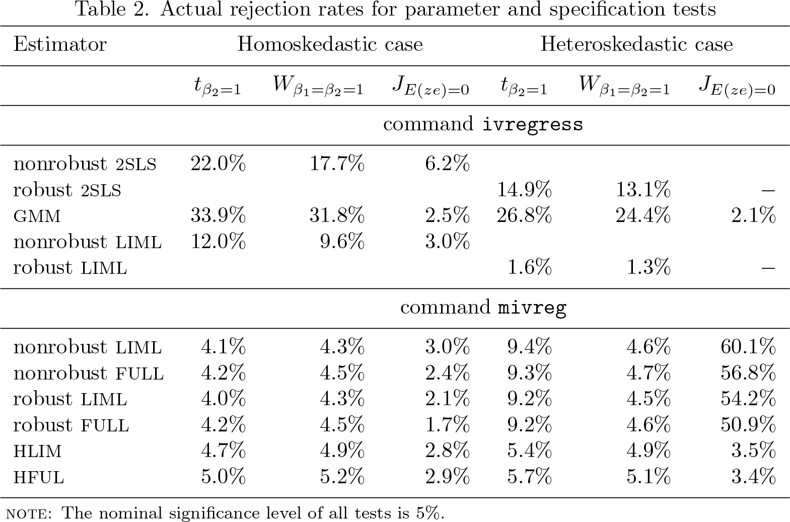
Table 2 contains actual rejection rates corresponding to the 5% nominal rate for the two-sided t test of the null H ₀ : β ₂ = 1 marked as t_{β 2 =1}, the Wald test of the null H ₀ : β ₁ = β ₂ = 1 marked as W_{β 1 = β 2 =1}, and the specification test marked as JE(ze)=0. The 2SLS and LIML tests produced by ivregress come in two forms: nonrobust and robust to heteroskedasticity. In the specification tests (which are available only for efficient estimators), the Basmann (1957) variance estimator is used. The test statistics produced by mivreg use the following estimators and robustness regimes: ² nonrobust LIML, nonrobust FULL, robust LIML, robust FULL, HLIM, and HFUL.

Table 2.

2. Actual rejection rates for parameter and specification tests

Estimator		Homoskedastic case						Heteroskedastic case
		tβ 2 =1		Wβ 1 = β 2 =1		JE(ze)=0		tβ 2 =1		Wβ 1 = β 2 =1		JE(ze)=0
command <mono>ivregress</mono>
nonrobust 2SLS		22.0%		17.7%		6.2%
robust 2SLS								14.9%		13.1%		−
GMM		33.9%		31.8%		2.5%		26.8%		24.4%		2.1%
nonrobust LIML		12.0%		9.6%		3.0%
robust LIML								1.6%		1.3%		−
command <mono>mivreg</mono>
nonrobust	LIML		4.1%		4.3%		3.0%		9.4%		4.6%		60.1%
nonrobust	FULL		4.2%		4.5%		2.4%		9.3%		4.7%		56.8%
robust	LIML		4.0%		4.3%		2.1%		9.2%		4.5%		54.2%
robust	FULL		4.2%		4.5%		1.7%		9.2%		4.6%		50.9%
HLIM	4.7%		4.9%		2.8%		5.4%		4.9%		3.5%
HFUL	5.0%		5.2%		2.9%		5.7%		5.1%		3.4%

NOTE: The nominal significance level of all tests is 5%.

As expected, severe size distortions are exhibited by conventional parameter tests based on 2SLS, GMM, and LIML. ³ In the homoskedastic case, all the mivreg tests exhibit similar behavior with much smaller distortions, though the “heteroskedastic” versions seem to be more reliable. In the heteroskedastic case, the latter are the only valid ones theoretically and do deliver rejection rates close to nominal. The Fuller correction does not significantly affect these rejection rates. The results of specification testing point at huge distortions if one relies on “homoskedastic” specification tests when in fact the homoskedasticity assumption is violated. One must avoid using them in heteroskedastic environments because one is too likely to receive a signal of instrument invalidity when in fact the instruments are valid.

7 Example with real data

We illustrate the use of mivreg using real data from a well-known application to the married female labor supply (Mroz 1987). The number of observations is 428. ⁴

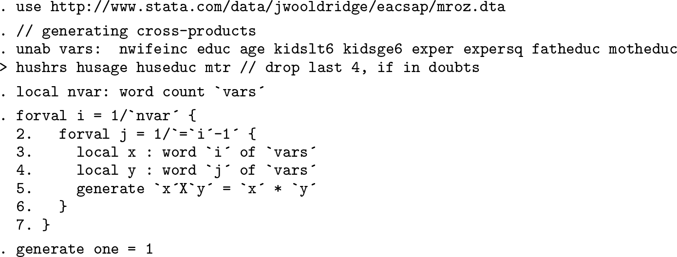
The left-side variable is working hours (hours), and the only endogenous right-side variable is log wages (lwage); there are also six exogenous controls: nwifeinc, educ, age, kidslt6, kidsge6, and the constant one. The list of basic instruments includes, in addition to the 6 exogenous controls, 8 exogenous variables: exper, expersq, fatheduc, motheduc, hushrs, husage, huseduc, and mtr, resulting in 14 instruments in total. The basic instruments are strong as a group: the first-stage F statistic equals 183.5. We also consider an extended set of instruments—the basic instruments plus all of their cross-products (“interactions”), the total numerosity amounting to 92. The use of the extended instrument set is meant to possibly enhance estimation efficiency by exploiting information in the instruments more actively. However, while the conventional tools are suitable for the basic set of instruments, the extended instrument set evidently requires handling via many-instrument asymptotics. The ratio of the number of instruments to the sample size is sizable: ℓ/n ≈ 0.215.

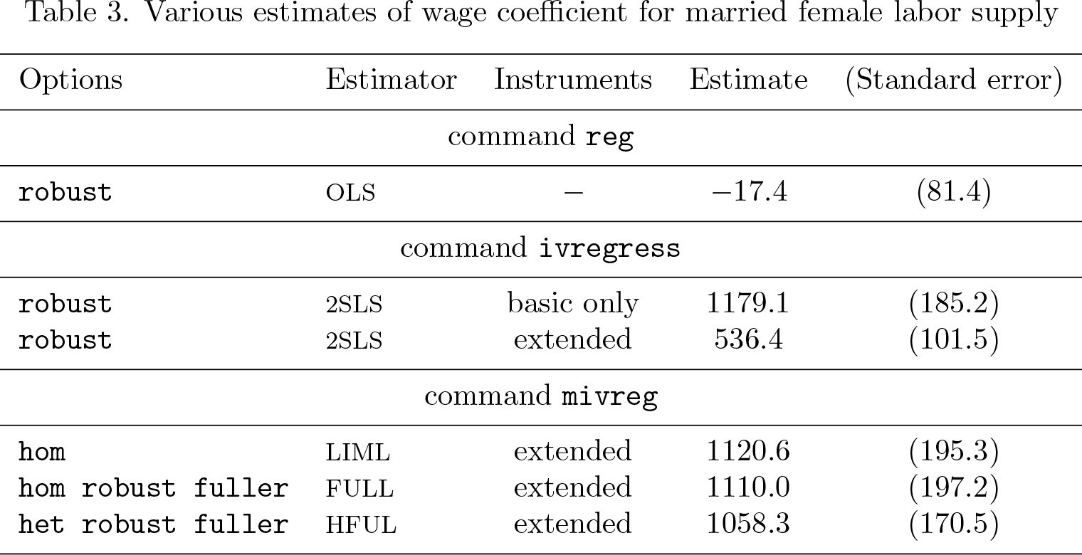
Table 3 presents various estimates for the slope coefficient of log wages: OLS, heteroskedasticity-robust 2SLS (using the basic and extended instrument sets), and three many-instrument-robust estimators—LIML, FULL, and HFUL (using the extended instrument set)—whose output will appear below.

Table 3.

3. Various estimates of wage coefficient for married female labor supply

Options	Estimator	Instruments	Estimate	(Standard error)
command <mono>reg</mono>
<mono>robust </mono>	OLS	−	−17.4	(81.4)
command <mono>ivregress</mono>
<mono>robust </mono>	2SLS	basic only	1179.1	(185.2)
<mono>robust </mono>	2SLS	extended	536.4	(101.5)
command <mono>mivreg</mono>
<mono>hom </mono>	LIML	extended	1120.6	(195.3)
<mono>hom robust fuller </mono>	FULL	extended	1110.0	(197.2)
<mono>het robust fuller </mono>	HFUL	extended	1058.3	(170.5)

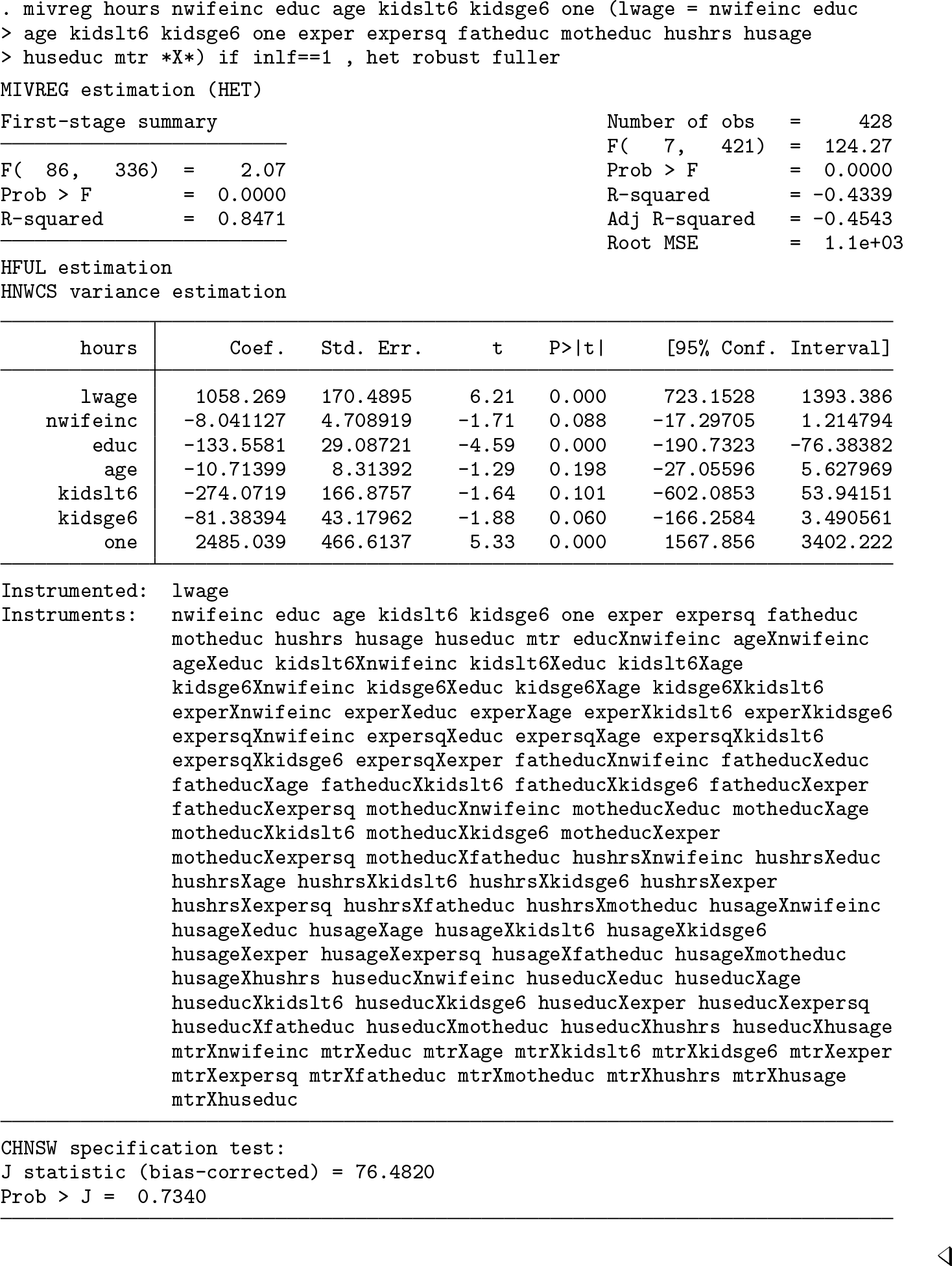
Evidently, because of unaccounted endogeneity, OLS estimation from applying the reg command is inconsistent; the numerical value of the OLS estimate is even negative, revealing a big endogeneity bias. The (more than twofold!) difference between the two 2SLS estimates points at invalidity of conventional tools and the ivregress command when instruments are many. The LIML, FULL, and HFUL point estimates produced by the mivreg command are quite in line with the 2SLS estimate that uses only the basic instruments. ⁵ There is a small difference between “homoskedastic” LIML and FULL point estimates and the “heteroskedastic” HLIM point estimate. Though not too big, this difference makes the HFUL estimate more trustworthy. ⁶ The smaller standard error of HLIM compared with that of 2SLS may be interpreted as a gain in efficiency from using the extended instrument set.

The outputs produced by the command mivreg to deliver the three many-instrument-robust estimators appear next.

► Example

The output for LIML estimation with the option hom:

► Example

The output for FULL estimation with the options hom, robust, and fuller is as follows:

► Example

The output for HFUL estimation with the options het, robust, and fuller:

9 Programs and supplemental materials

Supplemental Material, st0580 - Many instruments: Implementation in Stata

Supplemental Material, st0580 for Many instruments: Implementation in Stata by Stanislav Anatolyev and Alena Skolkova in The Stata Journal