vcemway: A one-stop solution for robust inference with multiway clustering

Abstract

Most Stata commands allow cluster(varname) or vce(cluster clustvar) as an option, popularizing the use of standard errors that are robust to oneway clustering. For adjusting standard errors for multiway clustering, there is no solution that is as widely applicable. While several community-contributed packages support multiway clustering, each package is compatible only with a subset of models that Stata’s ever-expanding library of commands allows the researcher to fit. We introduce a command, vcemway, that provides a one-stop solution for multiway clustering. vcemway works with any estimation command that allows cluster(varname) as an option, and it adjusts standard errors, individual significance statistics, and confidence intervals in output tables for multiway clustering in specified dimensions. The covariance matrix used in making this adjustment is stored in e(V), meaning that any subsequent call to postestimation commands that use e(V) as input (for example, test and margins) will also produce results that are robust to multiway clustering.

1 Introduction

The use of one-way clustered standard errors in empirical research is now commonplace. Compared with usual heteroskedasticity-robust standard errors, which assume the independence of regression errors across all observations, clustered standard errors offer an extra layer of robustness by allowing for correlations across observations that belong to the same cluster. In the analysis of a labor-force panel survey, for example, repeated observations on an individual may form a cluster, and standard errors may be clustered at the individual level to attain robustness to within-individual correlations over time. Cameron and Miller (2015) provide a masterful review of the methods and literature.

In recent years, the use of multiway clustered standard errors has also received growing attention. This extension robustifies one-way clustered standard errors further by allowing for other clusters within which regression errors may be correlated. For example, in the analysis of panel data on bilateral trade flows, two-way clustering may make standard errors robust to within-country correlation and within-country pair correlation over time (Cameron, Gelbach, and Miller 2011). In labor economics, Dube, Lester, and Reich (2010, 2016) analyze earnings and employment data on pairs of U.S. counties that share state border segments, and they apply two-way clustering to account for within-state correlations and within-border segment correlations. In the analysis of firm-level panel data in finance, Thompson (2011) has pioneered the use of two-way clustering that accounts for within-firm correlations over time and within-time period correlations across firms. Gow, Ormazabal, and Taylor (2010) show that many well-known findings in the accounting literature may be sensitive to the use of two-way clustering that similarly accounts for within-firm and within-time period correlations.

Most Stata commands allow cluster(varname) or vce(cluster clustvar) as an option, facilitating and popularizing the use of one-way clustered standard errors. No similar one-stop solution is available for multiway clustering. Popular communitycontributed commands such as cmgreg (Gelbach and Miller 2009), ivreg2 (Baum, Schaffer, and Stillman 2002), and reghdfe (Correia 2014) support multiway clustering, but only with specific models (for example, cmgreg with regress; ivreg2 with ivregress; and reghdfe with areg, xtreg, fe, and xtivreg, fe). The versatile boottest package (Roodman et al. 2019) supports multiway clustering with all aforementioned models as well as nonlinear models using ml maximize, but it still leaves out many commands that allow cluster(varname) as an option, such as xtreg, re and an ever-expanding library of community-contributed commands. Moreover, boottest does not store multiway clustered covariance matrices in e(V), meaning that it does not adjust for multiway clustering to postestimation commands such as margins and predictnl. ¹ In general, to apply robust inference with multiway clustering in a new context, Stata users may need to conduct a fresh search for a relevant command, which may not always exist.

In this article, we describe a simple approach to obtain almost any Stata command’s output with multiway clustered standard errors, and we describe a new command, vcemway, that automates the process. The main idea is to use ereturn repost to replace an active output’s covariance matrix, stored in e(V), with its multiway clustered counterpart that has been computed by the researcher. Computing a multiway clustered covariance matrix is relatively straightforward when the researcher can use cluster(varname) to adjust for one-way clustering in each dimension of interest separately.

The command vcemway provides a one-stop solution for multiway clustering in Stata, comparable with what option cluster(varname) already provides for one-way clustering. Specifically, vcemway works with any estimation command that allows cluster(varname) as an option. It has an intuitive syntax diagram and adjusts standard errors, individual significance statistics, and confidence intervals in output tables for multiway clustering in specified dimensions. The covariance matrix used in making this adjustment overwrites the estimation command’s e(V), meaning that any subsequent call to postestimation commands that use e(V) as input (for example, test, margins, and predictnl) will also produce results that are robust to multiway clustering.

2 Adjusting for multiway clustering

To facilitate discussion, let us suppose that the researcher is interested in running a linear regression of outcome y on two regressors X and Z by executing regress y X Z. The researcher is also interested in adjusting standard errors for clustering in m nonnested dimensions, identified by variables id1, id2,…, idm, respectively. Let $\mathbb{M}$ denote a set of all 2 ^m −1 distinct combinations of the m cluster variable names, including singletons. For example, when m = 2, there are 2 ² − 1 = 3 elements in $\mathbb{M}$ : id1, id2, and (id1, id2). When m = 3, there are 2 ³ − 1 = 7 elements in $\mathbb{M}$ : id1, id2, id3, (id1, id2), (id1, id3), (id2, id3), and (id1, id2, id3). Extensions to m ≥ 4 are straightforward.

Cameron, Gelbach, and Miller (2011) show that an asymptotically valid m-way clustered covariance matrix, V _mway , may be conveniently computed in Stata and other software packages that allow for one-way clustering. Specifically, V _mway can be obtained by combining 2^m − 1 one-way clustered covariance matrices as follows:

$V_{mway}={\displaystyle \sum _{g\in \text{M}}{(-\text{1})}^{\text{1}+}{{ }^{|}}^g{ }^{|}{V}_g}$

1

V _g is a covariance matrix adjusted for one-way clustering in “groups” formed by variables in g ∊ $\mathbb{M}$ , and |g| is the number of variables listed in g. The “groups” in this context are defined in the sense of Stata’s egen function group(varlist). For example, if g involves only one variable, say, g = id1, the groups coincide with the clusters identified by id1; executing regress y X Z, cluster(id1) stores V _g in e(V) of Stata’s ereturn results. If g involves two or more variables, say, g = (id1, id2), the groups can be identified by a new variable id1_id2 generated using egen id1_id2 = group(id1 id2); executing regress y X Z, cluster(id1_id2) stores V _g in e(V).

To see the algebraic structure of (1) more clearly, let us examine two-way (m = 2) and three-way (m = 3) clustering in detail. A two-way clustered covariance matrix is given by

$V_{mway}=V_{\text{id1}}+V_{\text{id2}}-V_{(\text{id1},\text{id2})}$

2

and a three-way clustered covariance matrix is given by

$V_{mway}=V_{\text{id1}}+V_{\text{id2}}+V_{\text{id3}}-V_{(\text{id1},\text{id2})}-V_{(\text{id1},\text{id3})}-V_{(\text{id2},\text{id3})}+V_{(\text{id1},\text{id2},\text{id3})}$

As these examples illustrate, the multiplication factor (−1)^{1+ | g |} in (1) means that V _g is added to the sum when g involves an odd number of variables and subtracted from the sum when g involves an even number of variables.

V _mway can be used to construct Wald statistics in the usual manner to draw inferences robust to m-way clustering. To construct t statistics, the researcher can obtain m-way clustered standard errors by taking the square roots of the diagonal entries in V _mway . Let n _c denote the number of clusters identified by variable c ∊ {id1, id2,…, idm}, that is, the number of distinct values in variable c, and G denote the minimum of these m cluster sizes, G = min(n _id1 , n _id2 ,…, n _{id m}). As G grows arbitrarily large, the usual asymptotic distributions apply: a Wald statistic testing q restrictions is approximately χ ²(q) distributed, and a t statistic is approximately standard normal. When G is small, there is no guaranteed method to improve finite-sample inference. One useful starting point would be to conduct F tests using F _q,G−1 critical values in lieu of the asymptotic Wald tests using χ ²(q) critical values and t tests using t _{G − 1} critical values in lieu of the standard normal critical values (Cameron, Gelbach, and Miller 2011; Cameron and Miller 2015).

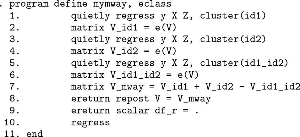
The results of Cameron, Gelbach, and Miller (2011) allow the researcher to write a relatively simple Stata program to robustify test statistics to m-way clustering. As a minimal example, consider the following program, mymway, that adjusts for two-way clustering on id1 and id2.

Lines 1–6 fit the linear regression model of interest, accounting for one-way clustering on each g ∊ $\mathbb{M}$ and create matrices to store each V _g. Line 7 combines the three stored matrices to compute an m-way clustered covariance matrix V_mway using (1), or more directly (2). Line 8 is an important step that replaces the active covariance matrix e(V) in Stata’s memory with V_mway; this allows the researcher to robustify test statistics produced by all existing postestimation commands, such as test, margins, and predictnl, to m-way clustering, without having to modify or rewrite such programs. Line 9 effectively sets the residual degrees of freedom to ∞, thereby requesting the use of asymptotic t tests and Wald tests; replacing df_r =. with df_r = # would request the use of t and F tests based on t _# and F _{q, #} critical values, where G − 1 mentioned in the preceding paragraph is one possible choice for integer #. Finally, line 10 reports the output of regress that has been modified to include m-way clustered standard errors as well as the corresponding asymptotic t statistics (or “z” statistics in Stata’s parlance) and confidence intervals. Once defined, the program can be executed by entering mymway at Stata’s command prompt.

While generalizing the minimal example to accommodate other estimation commands and clustering in m ≥ 3 dimensions is seemingly straightforward, there are several implementation issues that deserve close attention. First, repeatedly fitting the same model 2^m − 1 times may require substantial computer time, especially when the sample size is large or the estimation command of interest solves a complicated numerical optimization task. Whenever postestimation command predict can be used to compute observation-level residuals (for example, after regress) or scores (for example, after ml, maximize), Stata’s programming command robust can save time. ² Using the observation-level residuals or scores, robust can compute a covariance matrix adjusted for one-way clustering on varname, even when the preceding estimation run did not specify cluster(varname) as an option. This allows the researcher to execute the time-consuming step of fitting the model only once and compute each V _g subsequently via a simple algebraic task.

Second, the researcher should be on alert for the consequences of missing values in cluster identifiers. Continuing with the minimal example above, let us suppose that id1 has missing values for one set of observations and id2 has missing values for another set of observations, meaning their group variable id1_id2 has missing values for the union of the two sets. Then, each instance of regress in lines 1, 3, and 5 will use a different estimation sample, making the covariance matrix V_mway in line 7 invalid. A similar problem arises for robust because each one-way clustered covariance matrix will be computed over a different set of observations. Stata command markout makes it easy to define an estimation sample that excludes observations with missing values in any cluster identifier.

Third, using a one-way clustered covariance matrix produced by Stata’s built-in cluster(varname) as V _g is equivalent to adopting a particular small-cluster correction factor. As Cameron, Gelbach, and Miller (2011) point out, when computing V _g, Stata multiplies the underlying large-sample covariance formula by {n _g /(n _g − 1)} × {(N − 1)/(N − #)} to mitigate small-sample bias, where n _g is the number of clusters or groups identified by g ∊ $\mathbb{M}$ , N is the number of observations in the estimation sample, and # is the number of estimated coefficients for some commands (for example, regress) and 1 for others (for example, ml, maximize). Our minimal example and its possible extensions therefore apply a potentially different correction factor to each component matrix V _g of V _mway in the same manner as community-contributed command cmgreg (Gelbach and Miller 2009). Of course, the researcher may choose to apply the same correction factor to all component matrices. For example, communitycontributed command reghdfe applies a more conservative correction factor, specifically {G/(G − 1)} × {(N − 1)/(N − #)}, where G is the minimum cluster size defined above. Community-contributed command ivreg2 also applies this conservative factor when option small is specified; otherwise, it uses a large-sample formula directly without any small-sample correction.

Fourth, Cameron, Gelbach, and Miller (2011) point out that in some applications, V _mway based on (1) may not be positive semidefinite. As a solution, they suggest that the researcher may replace negative eigenvalues of V _mway with 0s and reconstruct the covariance matrix using the updated eigenvalues and the original eigenvectors. By taking advantage of Stata’s Mata environment, this approach can be implemented by inserting the following command lines between lines 7 and 8 in the minimal example.

. mata: symeigensystem(st_matrix("V_mway"), EVEC = ., eval = .)

. mata: eval = eval :* (eval :> 0)

. mata: st_matrix("V_mway", EVEC*diag(eval)*EVEC´)

In section 3, we will introduce the command vcemway, which generalizes the minimal example above, accounting for the major implementation issues. Before proceeding, remember that like one-way clustering, multiway clustering should be applied with careful attention to the model of interest. For example, in nonlinear models such as probit, the presence of cluster-specific random effects is a form of model misspecification that can render parametric estimators inconsistent; it would be inappropriate to consider probit with multiway clustered standard errors as a substitute for a more fundamental modeling solution such as the crossed random-effects probit model that meprobit supports. Cameron and Miller (2015, sec. VII.C) and references therein provide further information on cluster–robust inferences in nonlinear models.

Even for linear models, the potential limitations of multiway clustering should be recognized. A prominent example arises in the analysis of paired or “dyadic” data such as bilateral trade-flow data, where each observation is on a distinct country pair, {A, B}. While two-way clustering on variables identifying A and B adjusts for error correlation in {Australia, Canada} and {Australia, USA} and in {USA, UK} and {Canada, UK}, it fails to account for correlation in {Australia, USA} and {USA, UK}; the last two country pairs share neither A nor B because USA appears in alternate positions. More general clustering methods for dyadic data have been developed by Aronow, Samii, and Assenova (2015) and Cameron and Miller (2014).

For linear models with multiway fixed effects, Correia (2015) advises that the researcher should drop singleton groups in each dimension of fixed effects iteratively until no singleton group remains, before clustering standard errors in those dimensions or upper dimensions that nest them (for example, county-level fixed effects and state-level clustering). Including singleton groups that comprise one observation may have undue effects on statistical inference by making small-sample correction factors smaller than otherwise, even though they have no effect on coefficient estimates and large-sample covariance formulas. Correia’s (2015) community-contributed command reghdfe allows for multiway clustering for linear models with multiway fixed effects and automates this advice.

3 The vcemway command: A one-stop solution for multiway clustering

vcemway is a new community-contributed command that automates the multiway clustering approach described in section 2. The researcher can apply vcemway to any existing estimation command that allows one-way clustering via cluster(varname) as an option and obtain standard errors and a covariance matrix that have been adjusted for clustering in m ≥ 2 dimensions.

vcemway expands on our minimal example in section 2, mymway, to provide a convenient tool that addresses the implementation issues that we had subsequently discussed. When predict can be applied to compute observation-level residuals or scores for the estimation command of interest, vcemway speeds up execution time by avoiding repeated estimation of the same model with iterative one-way clustering; instead, it uses robust to obtain the component matrices V _g of (1). ³ vcemway builds in a sample marker that ensures that every component matrix is computed using the same estimation sample, specifically a set of observations in which none of the m cluster identifiers is missing. When the resulting m-way clustered covariance matrix V _mway is not positive semidefi- nite, vcemway reconstructs the matrix after replacing its negative eigenvalues with zeros and displays a telltale warning message. Finally, vcemway offers options that allow the researcher to choose his or her preferred small-sample adjustment factor and customize the residual degrees of freedom for t and F tests.

3.1 Syntax

The syntax for vcemway is

vcemway cmdline_main , cluster( varlist ) vmcfactor( type ) vmdfr( # ) cmdline_options

3.2 Options

cluster(varlist) accepts varlist that lists the names of m ≥ 2 variables that identify the clustering dimensions of interest. As we will explain shortly, the optional options vmcfactor() and vmdfr() allow the researcher to supply his or her preferred small-sample correction factor and residual degrees of freedom. In the remaining syntax diagram, cmdline_main refers to the main component of an estimation command line that the researcher would like to execute, such as xtreg y X Z; and cmdline_options refers to required and optional options in that command line, such as re and nonest. To complete this example, we see that executing vcemway xtreg y X Z, cluster(id1 id2 id3) re nonest will report a linear random-effects regression, with standard errors that have been adjusted for clustering in the three variables and computed using the default settings (see below) for the options vmcfactor() and vmdfr(). cluster() is required.

vmcfactor(type) specifies the type of small-cluster correction factor that vcemway applies to the component covariance matrices V _g of (1). type may be default, minimum, or none. Recall that each component matrix V _g of (1) is a one-way clustered covariance matrix. When computing V _g, Stata incorporates a small-sample correction factor of {n _g /(n _g − 1)} × {(N − 1)/(N − #)}, where n _g is the number of clusters or groups identified by g ∊ $\mathbb{M}$ , N is the number of observations in the estimation sample, and # is the number of estimated coefficients for some commands (for example, regress) and 1 for others (for example, ml, maximize). The small-cluster correction factor henceforth refers to the first term in the product, n _g /(n _g − 1).

Unless specified otherwise, vcemway assumes the default type that uses Stata’s oneway clustered covariance matrices without further modification. That is, each V _g incorporates its own small-cluster correction factor of n _g /(n _g − 1).

The minimum type requests the use of a conservative correction factor that is identical across all component matrices. Specifically, every V _g is recalculated by replacing n _g /(n _g −1) with G/(G−1), where G is the size of the smallest clustering dimension.

For instance, suppose that cluster(id1 id2 id3) has been specified and there are 180, 30, and 78 clusters in id1, id2, and id3, respectively. G will be 30 in this case.

Finally, the none type requests the use of no small-cluster correction. In this case, every V _g is recalculated by replacing n _g /(n _g − 1) with 1.

vmdfr(#) specifies the residual degrees of freedom for t and F tests. The default setting varies from command to command. In case the estimation command in question reports large-sample test statistics (for example, ivregress and ml, maximize), # is set to missing so that the researcher can carry out the large-sample tests instead of t and F tests. In case the estimation command reports small-sample statistics (for example, regress), # is set to (G−1), where G is the size of the smallest clustering dimension.

cmdline_options specifies required and optional options in that command line, such as re or fe. To complete this example, we see that executing vcemway xtreg y X Z, cluster(id1 id2 id3) re nonest will report a linear random-effects regression, with standard errors adjusted for three-way clustering.

4 Examples

Consider nlswork.dta used by examples in Stata’s help menu for xtreg. This file provides a panel dataset wherein variable idcode identifies individuals and variable year identifies survey years. We will fit a linear regression model that specifies the logarithm of an individual’s wage (ln_wage) as a function of years of schooling (grade), work experience (ttl_exp), and squared work experience. The following example applies vcemway with regress to compute the ordinary least-squares (OLS) estimates of this model with standard errors adjusted for two-way clustering in idcode and year.

At the end of the usual output table, vcemway includes notes to convey key information concerning its implementation. ⁴ While one cannot tell from the output log in black and white, the notes display vcemway and test as blue-colored hyperlinks to the relevant help files. Options vmcfactor() and vmdfr() will change these notes in an expected manner. For example, vmcfactor(minimum) will induce vcemway to report that The small-cluster correction factor is G/(G-1) where G = 15, the minimum of 2 cluster sizes. The null hypothesis for the joint test statistic (for example, F test above) that Stata reports as part of an output table is command specific, and automatically identifying the null is a difficult task; vcemway therefore does not attempt to update that part of Stata output. Nevertheless, because postestimation commands after vcemway will make use of a multiway clustered covariance matrix, the researcher can use test to carry out a multiway clustered version of the relevant joint hypothesis test.

For comparison, consider the following two command lines that produce t statistics that are robust to clustering only in one of the two dimensions at a time.

. regress ln_w grade ttl_exp c.ttl_exp#c.ttl_exp, cluster(idcode) (output omitted )

. regress ln_w grade ttl_exp c.ttl_exp#c.ttl_exp, cluster(year) (output omitted )

With adjustment for one-way clustering on idcode, the t statistics are 33.83, 18.71, −4.32, and 19.31, from grade to cons. With adjustment for one-way clustering on year, the t statistics are 31.07, 6.07, −1.56, and 27.25, in the same order. Thus, each two-way clustered t statistic, shown in the output table above, is smaller than either of its one-way clustered counterparts. In general, whether multiway clustering leads to smaller t statistics (or equivalently, larger standard errors) than one-way clustering is an empirical question that cannot be answered ex ante. Cameron, Gelbach, and Miller (2011, sec. 4) provide several empirical applications comparing two-way clustering to one-way clustering. In those applications, two-way clustered standard errors turn out to be larger than the average of two one-way clustered standard errors, and sometimes they also turn out to be larger than both one-way clustered standard errors as in the present example.

Applying vcemway alongside estimation commands that have more complex syntax diagrams is equally straightforward. For illustration, we will extend the OLS regression above to incorporate random effects at the individual level (that is, idcode level). The following example estimates the resulting random-effects model and adjusts its standard errors for two-way clustering in idcode and year. Because the model accounts for idcode-level random effects and year is not nested in idcode, the researcher must specify xtreg‘s native nonest option to allow Stata to produce a covariance matrix adjusted for clustering in year.

For comparison, consider one-way clustered z statistics obtained by executing the following command lines:

. xtreg ln_w grade ttl_exp c.ttl_exp#c.ttl_exp, cluster(idcode) re (output omitted )

. xtreg ln_w grade ttl_exp c.ttl_exp#c.ttl_exp, cluster(year) re nonest (output omitted )

With adjustment for one-way clustering on idcode, the z statistics are 35.06, 24.24, −8.94, and 19.89 from grade to cons. With adjustment for one-way clustering on year, the z statistics are 15.92, 7.79, −2.73, and 9.47, respectively. As in the OLS example above, two-way clustering leads to more conservative inferences (that is, smaller z statistics) than either of the one-way clustering approaches.

6 Programs and supplemental materials

Supplemental Material, st0582 - vcemway: A one-stop solution for robust inference with multiway clustering

Supplemental Material, st0582 for vcemway: A one-stop solution for robust inference with multiway clustering by Ariel Gu and Hong Il Yoo in The Stata Journal

References

1.
AronowP. M.SamiiC.AssenovaV. A.2015. Cluster–robust variance estimation for dyadic data. Political Analysis23: 564–577.
2.
BaumC. F.SchafferM. E.StillmanS.2002. ivreg2: Stata module for extended instrumental variables/2SLS and GMM estimation. Statistical Software Components S425401, Department of Economics, Boston College. https://ideas.repec.org/c/boc/bocode/s425401.html.
3.
CameronA. C.GelbachJ. B.MillerD. L.2011. Robust inference with multiway clustering. Journal of Business & Economic Statistics29: 238–249.
CameronA. C.2015. A practitioner’s guide to cluster–robust inference. Journal of Human Resources50: 317–372.
6.
CorreiaS.2014. reghdfe: Stata module to perform linear or instrumental-variable regression absorbing any number of high-dimensional fixed effects. Statistical Software Components S457874, Department of Economics, Boston College. https://ideas.repec.org/c/boc/bocode/s457874.html.
DubeA.LesterT. W.ReichM.2010. Minimum wage effects across state borders: Estimates using contiguous counties. Review of Economics and Statistics92: 945–964.
9.
DubeA.2016. Minimum wage shocks, employment flows, and labor market frictions. Journal of Labor Economics34: 663–704.
GowI. D.OrmazabalG.TaylorD. J.2010. Correcting for cross-sectional and time-series dependence in accounting research. Accounting Review85: 483–512.
12.
RoodmanD.MacKinnonJ. G.NielsenM. Ø.WebbM. D.2019. Fast and wild: Bootstrap inference in Stata using boottest. Stata Journal19: 4–60.
13.
ThompsonS. B.2011. Simple formulas for standard errors that cluster by both firm and time. Journal of Financial Economics99: 1–10.
Supplementary Material
Please find the following supplemental material available below.
For Open Access articles published under a Creative Commons License, all supplemental material carries the same license as the article it is associated with.
For non-Open Access articles published, all supplemental material carries a non-exclusive license, and permission requests for re-use of supplemental material or any part of supplemental material shall be sent directly to the copyright owner as specified in the copyright notice associated with the article.