Grade functions

Abstract

Student grade processing using Stata is more reliable than methods like spreadsheets and saves the user timeh, especially when courses are repeated. In this article, I introduce functions that automate some useful grade calculations: the functions curve grades according to combinations of a target grade mean, maximum, standard deviation, and percentile cutoff; convert between numerical grades and letter grades; and convert between 0–100 grades and 0–4 grades (grade point average). The functions can also convert between other grading scales, such as those used in other countries.

1 Introduction

I used to curve my course grades with complicated spreadsheets, which I had to modify for every class. When asked by a student when her grade would be available, I mentioned this cumbersome process. The student, who was taking my Stata class, asked why I did not curve my grades in Stata. Good question!

Calculating and curving grades taps into three of Stata’s strengths. First, calculation by do-file script is vastly more reliable and traceable than calculation by spreadsheet with its obscured cell-specific formulas. Students care whether grades are calculated reliably! Second, once the code is written, it can be reused every time the course is taught and modified for other courses, allowing for rapid processing of grades. Students care how quickly grades are posted! Third, Stata makes it easy to customize the process, such as automatically downloading data from a learning management system and saving the results in a clean spreadsheet. Teachers like their grade processing to be quick and easy!

Curving grades frees the test maker from worrying about whether the test is harder or easier than in previous years and whether the points on the test add up to 100. Maybe the grader wants to ensure that exactly half the class gets a grade of B or better. The functions in this package automate these conversions.

Curving raw scores with a z score transformation allows the grader to set the desired mean score and desired level of dispersion. This is typically done manually by setting the target mean and then adjusting the standard deviation by trial and error to achieve the desired maximum grade. The first function in this package, grade_curve(), automatically figures out the standard deviation required for a specified maximum grade. Alternatively, the user can directly choose a target mean and standard deviation or a target maximum grade and standard deviation.

The second function in this package, grade_pct(), curves grades according to a target percentage of grades above a certain cutoff. For example, one might want 15% of the grades to be at or above 90, that is, 15% in the A range. However, the cutoff and percentage targets alone are not sufficient to determine the distribution of grades. A lower mean grade and a bigger standard deviation could have the same percent above the cutoff as a higher mean grade with a smaller standard deviation (visualize the two distributions with the same cutoff). So the curve requires a target mean, maximum, or standard deviation in addition to the target percentage and cutoff.

grade_pct() is useful when there is an outlier high grade, which will cause a target maximum grade to skew the rest of the grades too low. Using grade_pct() keeps the outlier grade from “ruining the curve”, which students seem to fear so much. ¹

There is no objective answer for which parameters provide the best distribution for the curved grades, but curving the grades using these functions ensures that the transformed grades have logical consistency, whichever parameters are selected.

Once the grades are curved, typically on a 0 to 100 scale, one often wants to convert them to letter grades. gradetoAF() converts 0–100 grades to A–F grades, with or without pluses and minuses. Grades can also be converted to the 0 to 4 scale with the gradeto04() function.

Two additional functions convert grades in the other direction. gradeofAF() converts letter grades to the 0–100 scale, and gradeof04() converts from 0–4 grades to 0–100 grades.

With the use of options, gradetoAF() and gradeofAF() can convert between any user-specified numeric scale and grading symbols, such as those used in non-U.S. settings. The grade-curving functions grade_curve() and grade_pct() are already scale agnostic, so they can be applied to any grading system.

2 Syntax

2.1 grade_curve()

Description

grade_curve() curves grades with a z score transformation to produce curved grades that have a target mean and maximum grade, a target mean and standard deviation, or a target maximum grade and standard deviation. Because few of us think in terms of standard deviations, most users will use the target mean and maximum grade as parameters.

The expression exp will typically be a varname containing raw grade scores.

If the maximum input score is an outlier, the user may want to choose a higher maximum target grade than usual (for example, higher than 100 for a 0–100 scale) to prevent the curve from being “ruined” by the high score. Alternatively, the user may instead want to use the grade_pct() function to specify a percentile cutoff value.

2.2 grade_pct()

Description

grade_pct() curves grades so that a certain percent of the grades will be above a cutoff value. For example, with the required options percent(15) cutoff(90), 15% of grades will be above a cutoff of 90. An additional parameter is required to fix the distribution of curved grades: the target mean, maximum, or standard deviation.

By specifying the percent of grades above the cutoff, the user is also fixing the percent of grades below the cutoff (85% below the cutoff with percent(15)). This can be useful if the grader wants to ensure a certain percentage of low grades. For example, percent(85) cutoff(60) means that 15% of students will fail if 60 is the minimum passing score.

The expression exp will typically be a varname containing raw grade scores.

2.3 gradetoAF()

Description

gradetoAF() converts numeric grades to letter grades (A through F). The default numeric grades range from 0 to 100. With options, gradetoAF() can convert numeric grades with other scales and assign symbols other than A to F.

gradetoAF() by default converts the following scores into letter grades:

Input range	Letter grade
$\left[96\frac{2}{3},\infty \right)$	A+
$\left[96\frac{2}{3},\hspace{0.17em}96\frac{2}{3}\right)$	A
$\left[90,\hspace{0.17em}93\frac{1}{3}\right)$	A−
$\left[86\frac{2}{3},90\right)$	B+
$\left[83\frac{1}{3},86\frac{2}{3}\right)$	B
$\left[80,83\frac{1}{3}\right)$	B−
$\left[76\frac{2}{3},80\right)$	C+
$\left[73\frac{1}{3},76\frac{2}{3}\right)$	C
$\left[70,73\frac{1}{3}\right)$	C−
$\left[66\frac{2}{3},70\right)$	D+
$\left[63\frac{1}{3},\hspace{0.17em}66\frac{2}{3}\right)$	D
$\left[60,63\frac{1}{3}\right)$	D−
[0, 60)	F

Options

noplusminus changes the conversion to the following:

Input range	Letter grade
[90, ∞)	A
[80, 90)	B
[70, 80)	C
[60, 70)	D
[0, 60)	F

grade04 interprets the input expression as a 0–4.5 score (grade point average) rather than a 0–100 score.

cutoffs( numlist ) changes the boundaries between letter grades. The default is cutoffs(0 60 70 80 90 100). cutoffs() requires an ascending numlist. There must be one more cutoff than the number of grade symbols, which by default is five. The first cutoff level is the minimum score that results in a nonmissing letter grade. Scores above the last cutoff level are assigned the highest grade. Unless the noplusminus option is invoked, the range between successive cutoff levels is divided by 3 with a plus (+) character added to the letter grade for scores in the first third of the range and a minus (−) character added for scores in the last third of the range.

gradesymbols( string ) changes the symbols assigned as letter grades. The default is gradesymbols(F D C B A). The symbols should be in order of the lowest to the highest grade and be one less in number than the cutoffs(). If the symbols have spaces in them, the symbols with spaces must be enclosed in quotation marks, as in an example below.

2.4 gradeofAF()

Description

gradeofAF() converts letter grades (A through F) to numeric grades.

By default, the numeric grades range from 0 to 100. With options, gradeofAF() can assign other numeric scales.

varname must be a string variable. For gradeofAF() to return a nonmissing value, the string must contain A+, A, A−, B+, B, B−, C+, C, C−, D+, D, D−, or F.

Options

grade04 converts letter grades to a score from 0 to 4.5 instead of 0 to 100. gradevalues( numlist ) assigns different scores for letter grades. The default is

gradevalues(55 65 75 85 95), with pluses and minuses assigned numeric grades one-third more or less than the gap between grades. With the option grade04, the default is gradevalues(0 1 2 3 4). gradevalues() must have five values corresponding to grades for F, D, C, B, and A.

2.5 gradeto04()

Description

gradeto04() converts grades ranging from 0 to 100 to grades ranging from 0 to 4.5.

2.6 gradeof04()

Description

gradeof04() converts grades ranging from 0 to 4.5 to grades ranging from 0 to 100.

3 Examples of grade functions in use

Most people will use these grade functions straightforwardly to curve grades and convert them from one scale to another. Here are some examples of this typical use as well as some examples using nonstandard grading systems.

Increasingly, grades are housed in learning manage system (LMS) software such as D2L or Moodle, but strangely, they usually cannot curve grades within the system. LMSs are capable of exporting grades to a spreadsheet, though, and once the grades have been liberated from the LMS, Stata’s powers can be harnessed to organize and streamline the processing of grades.

Consider some real exam scores in the accompanying spreadsheet grades.xlsx. If the spreadsheets were created by an LMS, it would probably be necessary to add more lines of Stata code to clean up extra text stuffed into the spreadsheet. rename using the group syntax (see help rename group) is often helpful for converting the variable names to something intelligible.

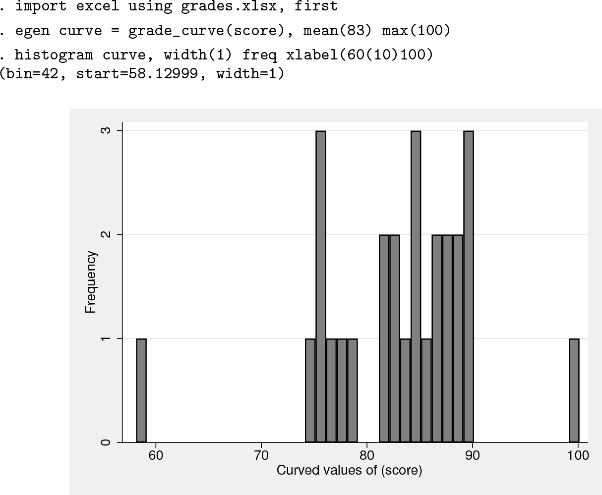
To curve the raw scores in variable score, let us choose a target mean grade of 83 and a maximum grade of 100. After loading the data, use the grade_curve() function to curve the grades with the desired mean and maximum, and graph the resulting distribution with histogram:

The histogram options width(), freq, and xlabel() are useful for displaying grades. The width(1) option ensures that each round-numbered grade will have a separate bar, the freq option shows the number rather than percent of students receiving each grade, and xlabel(60(10)100) shows the typical cutoffs for letter grades.

The histogram shows that the highest grade is an outlier, with a much higher score than the next highest grades (in both the raw scores in variable score and the curved grade in curve). If the scores are left as they are, only one student will receive a grade above 90.

To prevent the highest scorer from “ruining the curve”, keeping all the other students out of the over 90 range, I can increase the maximum score to a value greater than 100 to give more students a grade higher than 90. Setting the maximum grade at 105 causes 6 students to get a grade above 90.

It is not uncommon to assign students a grade of zero, only to find out later that they have dropped the course. If you do not want to include these students in the curve, add the condition if score>0 to the grade_curve() function:

grade_pct() is the appropriate function to use when the grader has a target percentage of students above a certain grade. To have 25% of students with a grade above 90, you must specify an additional parameter to determine the curve, usually the mean or maximum grade. Here the mean grade is specified as 83.

With grade_pct(), the outlier highest grade is automatically assigned a value above 100 without having to specify a high maximum grade manually as when using the function grade_curve().

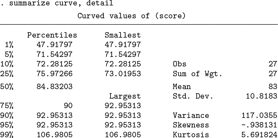
We can confirm that grade_pct() is meeting its target of 25% of grades at or above 90 with a mean of 83.

summarize shows that the 75th percentile is 90 and the mean grade is 83.

A referee suggested that some graders target a certain percentage of students to fail (rather Darwinian!), which is a target percent of grades below a cutoff. p% of grades above a cutoff implies 100 − p% of grades below the cutoff: 15% of students failing with a grade below 60 means that 85% of students received 60 or above. To ensure this distribution of grades, we can use the options percent(85) cutoff(60) and choose a maximum grade of 100:

For the grader who prefers to see a smoothed frequency distribution of grades, Stata’s kdensity command creates a more visually appealing graph than chunky histograms. The following graph shows the original and curved grades if 15% of students fail:

I will now create letter grades and 0–4 grades from the curved 0–100 grades:

To work with grading scales other than 0–100 or 0–4 numeric grades and A–F letter grades, I must modify the conversion functions with options. However, the curving functions (grade_curve() and grade_pct()) are scale agnostic and work with any numeric grading scale.

gradetoAF() has a number of options for converting into grade symbols other than A to F. For instance, if I want to use Greek letters, I can do this:

Note that this adds pluses and minuses to the Greek letters, which could be avoided with the noplusminus option.

More elaborately, I can include a new set of grade symbols and grade cutoffs that correspond to the boundaries between symbols. My sons used to study at a school that did not like conventional letter grades and felt descriptive phrases would reduce competitive pressures. The grade cutoffs nonetheless corresponded to the usual A–F scale. The following code converts numeric grades to this scale.

The following listing (after numeric formatting using the format command) shows the first five observations of each of the newly constructed variables.

After you reorder and pare down the variables, it is convenient to save the curved grades in a spreadsheet for future access or to load back into an LMS.

gradestoAF is a general function for assigning text values to ranges of numbers. Above, I changed the text values in the gradesymbols() option to Greek letters. In the following example, I will assign the A–F letter grades to a scoring system that ranges from 0–10 instead of 0–100 by specifying new numerical cutoff points in the cutoffs() option.

Vietnamese universities assign grades on a 0 to 10 scale. To make the grades more understandable to foreign degree programs, a Vietnamese university I collaborate with now includes A–F letter grades equivalent to the 0–10 grades in their transcripts. These could be calculated with the gradetoAF() function. The following code loads the 0–10 numeric grades from a spreadsheet and applies the appropriate numerical cutoff levels.

The final example uses the gradeofAF() function to convert letter grades back to numeric grades. I wrote this function because I received data on student performance as letter grades, and I needed to convert them to numeric scores for statistical analysis.

The plus and minus grade values assigned by gradeofAF() are equidistant between whole letter grades. By default, the numerical values for grades F, D, C, B, and A are 55, 65, 75, 85, and 95, respectively. That means B+ and A− will be equally spaced between 85 and 95, which rounded to one decimal place is 88.3 and 91.7. The numerical grade assigned to D− is as far below D as D+ is above D (because the values of an F typically range between 0 to 60), that is, 61.3.

The curved grades in the variable curved have mean value of 83 by construction. Converting curve into letter grades letter causes a loss of information because letter grades are less precise than numeric grades. Converting the grades in letter back to numeric using gradeofAF(), as above, causes the mean to be slightly lower at 82.9 and the standard deviation to also be lower than in curve. With another set of grades, the small changes in mean and variance might be positive or negative.

The next section explains the formulas and technical details behind the grade functions.

4 Methods and formulas

Let x denote the variable to “curve” or transform from one range to another. Let y be the curved result. Let x_i , i = 1,…, n, denote an individual observation of x, and let y_i denote an observation of y.

The mean of x_i , $\overline{x}$ , is

$\overline{x}=\frac{1}{n}{\displaystyle \sum _{i=1}^n{x}_i}$

The variance of x_i , $s_x^2$ , is

$s_x^2=\frac{1}{n-1}{\displaystyle \sum _{i=1}^n{\left(x_i-\overline{x}\right)}^2}$

The standard deviation of x_i , s_x , is the square root of the variance: $s_x=\sqrt{s_x^2}$ .

4.1 grade_curve()

The egen function grade_curve()performs a z score transformation to curve the values of x. grade_curve() first converts the x_i values into z scores, where

$z_i=\frac{x_i-\overline{x}}{s_x}$

z_i has a mean of

$\overline{z}=\frac{1}{n}{\displaystyle \sum _{i=1}^n{z}_i}=\frac{1}{n}{\displaystyle \sum _{i=1}^n\left(\frac{x_i-\overline{x}}{s_x}\right)}=\frac{\overline{x}-\overline{x}}{s_x}=0$

and a variance (and standard deviation) of

$s_z^2=\frac{1}{n-1}{\displaystyle \sum _{i=1}^n{z}_i^2}=\frac{1}{n-1}{\displaystyle \sum _{i=1}^n{\left(\frac{x_i-\overline{x}}{s_x}\right)}^2}={\left(\frac{x_i-\overline{x}}{s_x}\right)}^2=\frac{s_x^2}{s_x^2}=1$

The user of grade_curve() can specify three alternative pairs of parameters for the curved grades: the target mean and standard deviation, the mean and maximum grade, or the standard deviation and maximum.

Case 1: Specify the mean and standard deviation of curved grades

The user chooses a mean of µ and a standard deviation of σ as in egen y = grade_curve(x), mean( µ ) std( σ ). Then, y_i is defined as

$y_i=\sigma z_i+\mu$

As intended, y_i has a mean of

$\overline{y}=\frac{1}{n}{\displaystyle \sum _{i=1}^n\left(\sigma z_i+\mu \right)}=\mu$

and variance

$s_y^2=\frac{1}{n-1}{\displaystyle \sum _{i=1}^n{\left(y_i-\mu \right)}^2}=\frac{1}{n-1}{\displaystyle \sum _{i=1}^n{\left(\sigma z_i\right)}^2}={\sigma }^2{s}_z^2={\sigma }^2$

Case 2: Specify the mean and maximum grade

The user chooses a mean of µ and a maximum grade value of y _max, as in egen y = grade_curve(x), mean( µ ) max( y _max ).

Note that the transformation from x to z and from z to y preserves the ranking of the values. Let x _(i) be the ith largest value of the x_i so that x ₍₁₎ ≤ x ₍₂₎ ≤ · · · ≤ x _(i) ≤ · · · ≤ x _(n). Then x _(i) ≥ x _(i−1) ⇒ z _(i) ≥ z _(i−1) ⇒ y _(i) ≥ y _(i−1) because

$z_{\left(i\right)}=\frac{x_{\left(i\right)}-\overline{x}}{s_x}\ge \frac{x_{\left(i-1\right)}-\overline{x}}{s_x}=z_{\left(i-1\right)}$

and

$y_{\left(i\right)}=\sigma z_{\left(i\right)}+\mu \ge \sigma z_{\left(i-1\right)}+\mu =y_{\left(i-1\right)}$

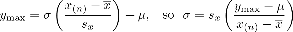
The preservation of rank means that the maximum grade y _max = y _(n) is the transformed value of the largest z score, z _(n), which in turn is the transformation of the largest x value, x _(n):

$y_{\left(n\right)}=\sigma z_{\left(n\right)}+\mu =y_{\max }\text{\hspace{0.17em}\hspace{0.17em}and\hspace{0.17em}}{z}_{\left(n\right)}=\frac{x_{\left(n\right)}-\overline{x}}{s_x}$

In this case, σ was not specified by the user, but the value of σ consistent with y _(n) = y _max is

$y_{\max }=\sigma \left(\frac{x_{\left(n\right)}-\overline{x}}{s_x}\right)+\mu ,\text{\hspace{0.17em}\hspace{0.17em}so\hspace{0.17em}\hspace{0.17em}}\sigma =s_x\left(\frac{y_{\max }-\mu }{x_{\left(n\right)}-\overline{x}}\right)$

With µ and σ in hand, we create y_i as in case 1, resulting in the highest grade y _(n) having the value y _max.

Case 3: Specify the maximum grade and the standard deviation

The user chooses a maximum grade value of y _max and a standard deviation of σ as in egen y = grade_curve(x), max( y _max ) std( σ ).

As in case 2,

$y_{\left(n\right)}=\sigma z_{\left(n\right)}+\mu =y_{\max }\text{\hspace{0.17em}\hspace{0.17em}and\hspace{0.17em}\hspace{0.17em}}{z}_{\left(n\right)}=\frac{x_{\left(n\right)}-\overline{x}}{s_x}$

but in this case, µ is unknown rather than σ. Solve for µ with

$y_{\max }=\sigma \left(\frac{x_{\left(n\right)}-\overline{x}}{s_x}\right)+\mu ,\text{\hspace{0.17em}\hspace{0.17em}so\hspace{0.17em}\hspace{0.17em}}\mu =y_{\max }-\sigma \left(\frac{x_{\left(n\right)}-\overline{x}}{s_x}\right)$

With µ and σ in hand, we create y_i as in case 1.

4.2 grade_pct()

The egen function grade_pct()requires a cutoff value, cut; a percentage of grades above the cutoff, p; and a third statistic: a mean µ, a maximum grade y _max, or a standard deviation σ. For example, the user could choose egen y = grade_pct(x), cutoff(90) percent(15) mean(80), meaning that the grades in y would assign 15% of the students grades 90 or above with a class mean of 80. Alternatively, egen y = grade_pct(x), cutoff(85) percent(30) max(100) would mean the grades in y would have 30% of grades at or above 85 with a maximum grade of 100.

Case 1: Specify the cutoff, the percentage, and the mean

The user chooses a cutoff value, cut; a percentage of grades above the cutoff, p; and a mean of µ as in egen y = grade_pct(x), cutoff( cut ) percent( p ) mean( µ ).

Let j be the largest value of i = 1,…, n such that j ≤ (1 − p/100)n. Then, x _(j) is the (100 − p)th percentile value of x_i . The standard deviation that is consistent with y _(j) being the pth percentile value of y_i and a mean grade of µ is

$\sigma =s_{\text{x}}\left(\frac{cut-\mu }{x_{\left(j\right)}-\overline{x}}\right)$

Then, y_i is defined as

$y_i=\frac{\sigma }{s_x}\left(x_i-\overline{x}\right)+\mu$

As shown above, the z score transform from x → y preserves the ranking, so y _(j), the (100 − p)th percentile value of y_i , is the transform of x _(j) and is equal to the cutoff value cut as intended:

$y_{\left(j\right)}=\frac{\sigma }{s_x}\left(x_{\left(j\right)}-\overline{x}\right)+\mu =\left(\frac{cut-\mu }{x_{\left(j\right)}-\overline{x}}\right)\left(x_{\left(j\right)}-\overline{x}\right)+\mu =cut$

Case 2: Specify the cutoff, the percentage, and the maximum grade

The user chooses a cutoff value, cut; a percentage of grades above the cutoff, p; and a maximum grade y _max as in egen y = grade_pct(x), cutoff( cut ) percent( p ) max( y _max ).

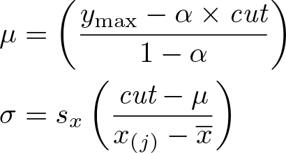
As before, let j be the largest value of i = 1,…, n such that j ≤ (1 − p/100)n, so that x _(j) is the (100 − p)th percentile value of x_i . To find the mean and standard deviation for y that is consistent with y _(j) being the (100 − p)th percentile value of y_i and a maximum grade of y _max, define

$\alpha =\left(\frac{x_{\left(n\right)}-\overline{x}}{x_{\left(j\right)}-\overline{x}}\right)$

where x _(n) is the maximum value of x. Then,

$\begin{array}{l}\mu =\left(\frac{y_{\max }-\alpha \times cut}{1-\alpha }\right)\\ \sigma =s_x\left(\frac{cut-\mu }{x_{\left(j\right)}-\overline{x}}\right)\end{array}$

and

$y_i=\frac{\sigma }{s_x}\left(x_i-\overline{x}\right)+\mu$

As in case 1,

$y_{\left(j\right)}=\left(\frac{cut-\mu }{x_{\left(j\right)}-\overline{x}}\right)\left(x_{\left(j\right)}-\overline{x}\right)+\mu =cut$

In addition,

$y_{\left(n\right)}=\frac{\sigma }{s_x}\left(x_{\left(n\right)}-\overline{x}\right)+\mu =\left(\frac{cut-\mu }{x_{\left(j\right)}-\overline{x}}\right)\left(x_{\left(n\right)}-\overline{x}\right)+\mu =\alpha \times cut+\left(1-\alpha \right)\mu =y_{\max }$

Case 3: Specify the cutoff, the percentage, and the standard deviation

This case will probably rarely be used but is included for completeness. The user chooses a cutoff value, cut; a percentage of grades above the cutoff, p; and a standard deviation σ as in egen y = grade_pct(x), cutoff( cut ) percent( p ) std( σ ).

The mean will be

$\mu =cut-\frac{\sigma }{s_x}\left(x_{\left(j\right)}-\overline{x}\right)$

where x _(j) is the (100 − p)th percentile value of x_i , and

$y_i=\frac{\sigma }{s_x}\left(x_i-\overline{x}\right)+\mu$

As intended,

$y_{\left(j\right)}=\frac{\sigma }{s_x}\left(x_{\left(j\right)}-\overline{x}\right)+cut-\frac{\sigma }{s_x}\left(x_{\left(j\right)}-\overline{x}\right)=cut$

4.3 gradetoAF()

The egen function gradetoAF() in its default configuration converts numeric grades ranging from 0 to 100 to letter grades ranging from F to A+. With options, other grading scales can be converted.

gradetoAF() assigns grades to a range of numerical cutoff values of variable x, as in egen letter = gradetoAF(x). Let the cutoff values be c ₀ , c ₁ ,…, c_M and the grade symbols be l ₁ , l ₂ ,…, l_M . The default cutoff values are 0, 60, 70, 80, 90, and 100 or can be specified with the option cutoff(). The default grade symbols are F, D, C, B, and A, or they can be specified with the option gradesymbols(). Notice that there must be one more cutoff value than grade symbols.

A grade of l_m is assigned to a new string variable if x ∊ [c_{m −1} , c_m ) for m = 1,…, M− 1. The last grade symbol l_M is assigned if x ∊ [c_{M −1}, .), that is, the interval including the final value c_M and all nonmissing higher values. Unless the noplusminus option is selected, the minus sign (−) is added to the grade symbol l_m if x ∊ [c_{m −1} , c_{m −1} + (c_m − c_{m −1})/3) for m = 2,…, M. The plus sign (+) is added to l_m if x ∊ [c_m − (c_m − c_{m −1})/3, c_m ) for m = 2,…, M − 1 and to l_M if x ∊ [c_M − (c_M − c_{M −1})/3, .).

4.4 gradeofAF()

The function gradeofAF() converts letter grades F to A+ to a numerical grade 0 to 100 or to a different numerical grade range if specified in options.

egen y = gradeofAF(gradelet) assigns a 0–100 value for each grade in gradelet, and with pluses and minuses, the grades are assigned values 1/3 more or less than the difference between grade values.

Let the five numerical values assigned to grades (F, D, C, B, A) be (v ₁ , v ₂ , v ₃ , v ₄ , v ₅). The default numerical values are (55, 65, 75, 85, 95), or they can be specified with the option gradevalues(). Let 1/3 of the difference between the grade values v2 through v5 be

$\begin{array}{l}{d}_{23}=(v_3-v_2)/3\\ d_{34}=(v_4-v_3)/3\\ d_{45}=(v_5-v_4)/3\end{array}$

The differences d ₂₃ , d ₃₄, and d ₄₅ are rounded to one decimal place for readability. Then, the mapping between grades and numerical values is

Grade	Value
F	v 1
D−	v 2 −d 23
D	v 2
D+	v 2 + d 23
C−	v 3 − d 23
C	v 3
C+	v 3 + d 34
B−	v 4 − d 34
B	v 4
B+	v 4 + d 45
A−	v 5 − d 45
A	v 5
A+	v 5 + d 45

4.5 gradeto04()

The function gradeto04() converts 0–100 grades to 0–4 grades.

The command egen y = gradeto04(x) assigns y = max{(x − 55)/10, 0}.

4.6 gradeof04()

The function gradeof04() converts 0–4 grades to 0–100 grades.

The command egen y = gradeof04(x) assigns y = 10x + 55.

5 Conclusion

I have found managing course grades in Stata to be much more efficient and reliable than my previous practice of using spreadsheets. I can reuse my scripts from one year to the next with almost no modification. The grade-curving and grade-conversion functions described here have made it simpler and faster to write my do-files. Now, when students ask when they can see their grades, I can say “later today”.

Supplemental Material

Supplemental Material, st0561 - Grade functions

Supplemental Material, st0561 for Grade functions by John Luke Gallup in The Stata Journal