Sage Journals: Discover world-class research

Abstract

Differences-in-differences evaluates the effect of a treatment. In its basic version, a “control group” is untreated at two dates, whereas a “treatment group” becomes fully treated at the second date. However, in many applications of this method, the treatment rate increases more only in the treatment group. In such fuzzy designs, de Chaisemartin and D’Haultfœuille (2018b, Review of Economic Studies 85: 999–1028) propose various estimands that identify local average and quantile treatment effects under different assumptions. They also propose estimands that can be used in applications with a nonbinary treatment, multiple periods, and groups and covariates. In this article, we present the command fuzzydid, which computes the various corresponding estimators. We illustrate the use of the command by revisiting Gentzkow, Shapiro, and Sinkinson (2011, American Economic Review 101: 2980–3018).

Keywords

st0560 fuzzydid differences-in-differences fuzzy designs local average treatment effects local quantile treatment effects

1 Introduction

Differences-in-differences (DID) is a method to evaluate the effect of a treatment when experimental data are not available. In its basic version, a “control group” is untreated at two dates, whereas a “treatment group” becomes fully treated at the second date. However, in many applications of the DID method, the treatment rate increases more in some groups than in others, but there is no group that goes from fully untreated to fully treated, and there is also no group that remains fully untreated. In such fuzzy designs, a popular estimator of treatment effects is the Wald DID, which is the DID of the outcome divided by the DID of the treatment.

As shown by de Chaisemartin and D’Haultfœuille (2018b), the Wald DID identifies a local average treatment effect (LATE) if two assumptions on treatment effects are satisfied. First, the effect of the treatment should not vary over time. Second, when the treatment increases both in the treatment and in the control group, treatment effects should be equal in these two groups. de Chaisemartin and D’Haultfœuille (2018b) also propose two alternative estimands of the same LATE. These estimands do not rely on any assumption on treatment effects, and they can be used when the share of treated units is stable in the control group. The time-corrected (TC) Wald ratio relies on common trends assumptions within subgroups of units sharing the same treatment at the first date. The changes-in-changes (CIC) Wald ratio generalizes the CIC estimand introduced by Athey and Imbens (2006) to fuzzy designs. Under the same assumptions as those used for the Wald CIC, local quantile treatment effects (LQTE) are also identified.

In this article, we describe the fuzzydid command, which computes the estimators corresponding to these estimands and performs inference on the LATE and LQTE using the bootstrap. When one computes standard errors and confidence intervals, clustering along one dimension can be allowed for. One can also perform equality tests between the Wald DID, Wald TC, Wald CIC, and placebo tests. This is important for choosing between these different estimands because they identify the LATE under different sets of assumptions.

The identification results mentioned above hold with a control group where the share of treated units does not change over time, a binary treatment, no covariates, two groups, and two periods. Nonetheless, they can be extended in several directions. First, under the same assumptions as those underlying the Wald TC estimand, the LATE of treatment group switchers can be bounded when the share of treated units changes over time in the control group. Second, nonbinary treatments can be easily handled by modifying the parameter of interest. Third, when the assumptions are more credible conditional on some controls, one can modify the Wald DID, Wald TC, and Wald CIC estimands to incorporate such controls. The fuzzydid command handles these extensions.

Finally, results can be extended to applications with multiple periods and groups that are prevalent in applied work. Researchers then estimate treatment effects via linear regressions, including time and group fixed effects. de Chaisemartin and D’Haultfœuille (2018a) show that around 19% of all empirical articles published by the American Economic Review between 2010 and 2012 use this research design. They also show that these regressions are extensions of the Wald DID to multiple periods and groups and that they identify weighted averages of LATEs with possibly many negative weights.¹ Thus, they do not satisfy the no-sign reversal property: the coefficient of the treatment variable in those regressions may be negative even if the treatment effect is positive for every unit in the population. On the other hand, the Wald DID, Wald TC, and Wald CIC estimands can be extended to applications with multiple groups and periods, and they then identify a LATE under the same assumptions as in the two groups and two periods case. Again, the fuzzydid command computes the corresponding estimators.

The remainder of the article is organized as follows. Section 2 presents the estimands and estimators considered by de Chaisemartin and D’Haultfœuille (2018b) in the simplest setup with two groups and periods, a binary treatment, and no covariates. Section 3 discusses the various extensions covered by the fuzzydid command. Section 4 presents fuzzydid. Section 5 illustrates fuzzydid by revisiting Gentzkow, Shapiro, and Sinkinson (2011), who estimate the effect of newspapers on electoral participation. Section 6 presents the finite sample performances of the various estimators through Monte Carlo simulations. Section 7 concludes.

2 Setup

2.1 Parameters of interest, assumptions, and estimands

We seek to identify the effect of a treatment D on some outcome. In this section, we assume that D is binary.² Y (1) and Y (0) denote the two potential outcomes of the same individual with and without treatment, while Y = Y (D) denotes the observed outcome. We assume the data can be divided into time periods represented by a random variable $T \in {0, . . ., \bar{t}}$ and into groups represented by a random variable $G \in {0, . . ., \bar{g}}$ . We start by considering the simple case where $\bar{t} = \bar{g} = 1$ , thus implying that there are two groups and two periods. In this case, G = 1 for units in the treatment group, and G = 0 for units in the control group, respectively.

We use the following notation hereafter. For any random variable R, S(R) denotes its support. R_gt and R_dgt are two other random variables such that R_gt ∼ R| G = g, T = t and R_dgt ∼ R| D = d, G = g, T = t, where ∼ denotes equality in distribution. For any event or random variable A, F_R and F_R _|A denote the cumulative distribution function (CDF) of R and its CDF conditional on A, respectively. Finally, for any increasing function F on the real line, we let F ⁻¹(q) = inf {x ∈ ℝ: F (x) ≥ q}. In particular, $F_{R}^{- 1}$ is the quantile function of R.

We maintain assumptions 1–3 below in most of this article.

Assumption 1. Fuzzy design

E (D_{11}) > E (D_{10}) and E (D_{11}) - E (D_{10}) > E (D_{01}) - E (D_{00})

Assumption 2. Stable percentage of treated units in the control group

For all d ∈ S(D), P (D ₀₁ = d) = P (D ₀₀ = d) ∈ (0, 1).

Assumption 3. Treatment participation equation

There exist $D (0), . . ., D (\bar{t})$ such that D = D(T ), D(t)⫫T |G $(t \in {0, . . ., \bar{t}})$ and for all $t \in {1, . . ., \bar{t}}$ ,

P {D (t) \geq D (t - 1) | G} = 1 or P {D (t) \leq D (t - 1) | G} = 1

In standard “sharp” designs, we have D = G × T , meaning that only observations in the treatment group and in period 1 get treated. With assumption 1, we consider instead “fuzzy” settings where D ≠ G × T in general but where the treatment group experiences a higher increase of its treatment rate between periods 0 and 1. Assumption 2 requires that the treatment rate remain constant in the control group and be strictly included between 0 and 1. This assumption is testable. Assumption 3 is equivalent to the latent index model $D = 1 {V \geq v_{G T}}$ (with V ⫫T |G) considered in de Chaisemartin and D’Haultfœuille (2018b). In repeated cross-sections, D(t) denotes the treatment status of a unit at period t, and only D = D(T ) is observed. In single cross-sections where cohort of birth plays the role of time, D(t) denotes instead the potential treatment of a unit had he or she been born at T = t. Here again, only D = D(T ) is observed.

We consider the subpopulation S = {D(0) < D(1), G = 1}, hereafter called the treatment group switchers. Our parameters of interest are their LATE and LQTE, which are, respectively, defined by

\begin{array}{l} Δ = E {Y (1) - Y (0) | S, T = 1} \\ τ_{q} = F_{Y (1) | S, T = 1}^{- 1} (q) - F_{Y (0) | S, T = 1}^{- 1} (q), q \in (0, 1) \end{array}

We introduce the main estimands in de Chaisemartin and D’Haultfœuille (2018b). We start by considering the three estimands of Δ. The first is the Wald DID defined by

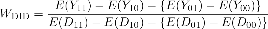
W_{DID} = \frac{E (Y_{11}) - E (Y_{10}) - {E (Y_{01}) - E (Y_{00})}}{E (D_{11}) - E (D_{10}) - {E (D_{01}) - E (D_{00})}}

W _DID is the coefficient of D in a two-stage least-squares regression of Y on D with G and T as included instruments and G × T as the excluded instrument.

The second estimand of Δ is the Wald TC ratio defined by

W_{TC} = \frac{E (Y_{11}) - E (Y_{10} + δ_{D_{10}})}{E (D_{11}) - E (D_{10})}

where δ_d = E(Y_d ₀₁) − E(Y_d ₀₀), for d ∈ S(D). Without the $δ_{D_{10}}$ term, W _TC would correspond to the coefficient of D in a two-stage least-squares regression of Y on D using T as the excluded instrument within the treatment group. δ ₀ and δ ₁ measure the evolution of the outcome among untreated and treated units in the control group, respectively. Under the assumption that these evolutions are the same in the two groups (see assumption 4’ below), the $δ_{D_{10}}$ term accounts for the effect of time on the outcome in the treatment group.

The third estimand of Δ is the Wald CIC defined by

W_{CIC} = \frac{E (Y_{11}) - E {Q_{D_{10}} (Y_{10})}}{E (D_{11}) - E (D_{10})}

where $Q_{d} (y) = F_{Y_{d 01}}^{- 1} \circ F_{Y_{d 00}} (y)$ is the quantile–quantile transform of Y from period 0 to 1 in the control group conditional on D = d. W _CIC is similar to W _TC except that it accounts for the effect of time on the outcome through the quantile–quantile transform instead of the additive term $δ_{D_{10}}$ .

Finally, we consider an estimand of τ_q . Let

F_{CIC, d} = \frac{P (D_{11} = d) F_{Y_{d 11}} - P (D_{10} = d) F_{Q_{d} (Y_{d 10})}}{P (D_{11} = d) - P (D_{10} = d)}

and

τ_{CIC, q} = F_{CIC, 1}^{- 1} (q) - F_{CIC, 0}^{- 1} (q)

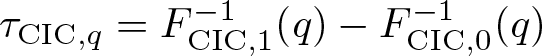
The estimands above identify Δ or τ_q under combinations of the following assumptions:

Assumption 4. Common trends

For all $t \in {1, . . ., \bar{t}}$ , E{Y (0)|G, T = t} − E{Y (0)|G, T = t − 1} does not depend on G.

Assumption 4’. Conditional common trends

For all d ∈ S(D) and all $t \in {1, . . ., \bar{t}}$ , E{Y (d)|G, T = t, D(t − 1) = d} − E{Y (d)|G, T = t − 1, D(t − 1) = d} does not depend on G.

Assumption 5. Stable treatment effect over time

For all d ∈ S(D) and all $t \in {1, . . ., \bar{t}}$ , E{Y (d) − Y (0)|G, T = t, D(t − 1) = d} = E{Y (d) − Y (0)|G, T = t − 1, D(t − 1) = d}.

Assumption 6. Monotonicity and time invariance of unobservables

Y (d) = h_d (U_d, T ), with U_d ∈ ℝ and h_d (u, t) strictly increasing in u for all (d, t) ∈ S(D) × S(T ). Moreover, U_d ⫫T |G, D(0).

Assumption 7. Data restrictions

$S (Y_{d g t}) = S (Y) = [\underline{y}, \bar{y}]$ with $- \infty \leq \underline{y} < \bar{y} \leq + \infty$ , for (d, g, t) ∈ S{(D, G, T )}.

$F_{Y_{d g t}}$ is continuous on ℝ and strictly increasing on S(Y), for (d, g, t) ∈ S{(D, G, T )}.

Assumption 4 is the usual common trends condition, under which the DID estimand identifies the average treatment effect on the treated in sharp designs where D = G×T . Assumption 4’ is a conditional version of this common trend condition, which requires that the means of Y (0) and Y (1) among untreated and treated units at period 0 follow the same evolution in both groups, respectively. Assumption 5 requires that in each group, the average treatment effect among units treated in period 0 remains stable between periods 0 and 1. Assumption 6 requires that potential outcomes be strictly increasing functions of a scalar and stationary unobserved term, as in Athey and Imbens (2006). Assumption 7 is a testable restriction on the distribution of Y that is necessary only for the Wald CIC and τ_q, _CIC estimands.

Theorem 1. (de Chaisemartin and D’Haultfœuille 2018b) Suppose that assumptions 1–3 hold.

If assumptions 4 and 5 also hold, then W _DID = Δ.

If assumptions 4’ also hold, then W _TC = Δ.

If assumptions 6–7 also hold, then W _CIC = Δ and τ_q, _CIC = τ_q .

Theorem 1 gives several sets of conditions under which we can identify Δ using one of the three estimands above. It also shows that τ_q can be identified under the same conditions as those under which the Wald CIC identifies Δ. Compared with the Wald DID, the Wald TC and Wald CIC do not rely on the stable treatment-effect assumption, which may be implausible. The choice between the Wald TC and the Wald CIC estimands should be based on the suitability of assumptions 4’ and 6 in the application under consideration. Assumption 4’ is not invariant to the scaling of the outcome, but it restricts only its mean. Assumption 6 is invariant to the scaling of the outcome, but it restricts its entire distribution. When the treatment and control groups have different outcome distributions conditional on D in the first period, the scaling of the outcome might have a large effect on the Wald TC. The Wald CIC is less sensitive to the scaling of the outcome, so using this estimand might be preferable. On the other hand, when the two groups have similar outcome distributions conditional on D in the first period, using the Wald TC might be preferable.

To test the assumptions underlying those estimands, one can test whether they are equal. If they are not, at least one of those assumptions must be violated. An alternative approach is to perform placebo tests. For instance, if three time periods are available (T = −1, 0, or 1) and if the treatment rate remains stable in both groups between T = −1 and 0, then the numerators of the Wald DID, Wald TC, and Wald CIC estimands for those two periods should be equal to 0.

2.2 Estimators

We now turn to the estimation of Δ and τ_q, _CIC using plugin estimators of the estimands above. Let (Y_i, D_i, G_i, T_i ) _i _=1…n denote an independent and identically distributed sample of (Y, D, G, T ) and define I _gt = {i : G_i = g, T_i = t} and I _dgt = {(i : D_i = d, G_i = g, T_i = t}. Let n_gt and n_dgt denote the size of I _gt and I _dgt for all d, g, t) ∈ S(D) × {0, 1}².

First, let

{\hat{W}}_{DID} = \frac{\frac{1}{n_{11}} \sum_{i \in I_{11}} Y_{i} - \frac{1}{n_{10}} \sum_{i \in I_{10}} Y_{i} - \frac{1}{n_{01}} \sum_{i \in I_{01}} Y_{i} + \frac{1}{n_{00}} \sum_{i \in I_{00}} Y_{i}}{\frac{1}{n_{11}} \sum_{i \in I_{11}} D_{i} - \frac{1}{n_{10}} \sum_{i \in I_{10}} D_{i} - \frac{1}{n_{01}} \sum_{i \in I_{01}} D_{i} + \frac{1}{n_{00}} \sum_{i \in I_{00}} D_{i}}

be the estimator of the Wald DID. Second, for any d ∈ S(D), let ${\hat{δ}}_{d} = (1 / n_{d}_{01}) \sum {_{i}}_{\in I_{d 01}} Y_{i} - (1 / n_{d}_{00}) \sum {_{i}}_{\in I_{d 00}} Y_{i}$ . Then, let

{\hat{W}}_{TC} = \frac{\frac{1}{n_{11}} \sum_{i \in I_{11}} Y_{i} - \frac{1}{n_{10}} \sum_{i \in I_{10}} (Y_{i} + {\hat{δ}}_{D_{i}})}{\frac{1}{n_{11}} \sum_{i \in I_{11}} D_{i} - \frac{1}{n_{10}} \sum_{i \in I_{10}} D_{i}}

be the estimator of the Wald TC. Third, for all (d, g, t) ∈ S(D) × {0, 1}², let ${\hat{F}}_{Y_{d g t}} (y) = 1 / n_{d g t} \sum {_{i}}_{\in I_{d g t}} 1 {Y_{i} \leq y}$ denote the empirical CDF of Y_dgt . Let

{\hat{Q}}_{d} (y) = m a x {{\hat{F}}_{Y_{d 01}}^{- 1} \circ {\hat{F}}_{Y_{d 00}}^{} (y), \min (Y_{i} : i \in I_{d 01})}

be the estimator of the quantile–quantile transform Q_d , and let

{\hat{W}}_{CIC} = \frac{\frac{1}{n_{11}} \sum_{i \in I_{11}} Y_{i} - \frac{1}{n_{10}} \sum_{i \in I_{10}} {\hat{Q}}_{D_{i}} (Y_{i})}{\frac{1}{n_{11}} \sum_{i \in I_{11}} D_{i} - \frac{1}{n_{10}} \sum_{i \in I_{10}} D_{i}}

be the estimator of the Wald CIC. Finally, let $\hat{P} (D_{g t} = d) = n_{d g t} / n_{g t}$ and

{\hat{F}}_{CIC, d}^{pi} = \frac{\hat{P} (D_{11} = d) {\hat{F}}_{Y_{d 11}} - \hat{P} (D_{10} = d) {\hat{F}}_{{\hat{Q}}_{d} (Y_{d 10})}}{\hat{P} (D_{11} = d) - \hat{P} (D_{10} = d)}

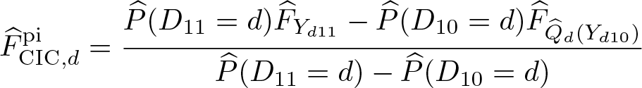
The function ${\hat{F}}_{CIC, d}^{pi}$ is the plugin estimator of FCIC,d, but it has the drawback of not being necessarily a proper CDF. It may not be nondecreasing and may not belong to [0, 1]. To avoid these issues, we consider a rearranged version ${\hat{F}}_{CIC, d}^{arr}$ of ${\hat{F}}_{CIC, d}^{pi}$ , following Chernozhukov, Fernández-Val, and Galichon (2010). Moreover, we let

{\hat{F}}_{CIC, d} (y) = max [min {{\hat{F}}_{CIC, d}^{arr} (y), 1}, 0]

With this proper CDF at hand, let

{\hat{τ}}_{q} = {\hat{F}}_{CIC, d}^{- 1} (q) - {\hat{F}}_{CIC, d}^{- 1} (q)

be the estimator of τ_q .

de Chaisemartin and D’Haultfœuille (2018b) show that ${\hat{W}}_{DID}$ , ${\hat{W}}_{TC}$ , ${\hat{W}}_{CIC}$ , and ${\hat{τ}}_{q}$ are root-n consistent and asymptotically normal under standard regularity conditions.³ de Chaisemartin and D’Haultfœuille (2018b) also establish the validity of the bootstrap to draw inference on Δ and τ_q based on these estimators. The fuzzydid command uses the bootstrap to compute the standard errors of all estimators and the percentile bootstrap to compute confidence intervals.

3 Extensions

3.1 Including covariates

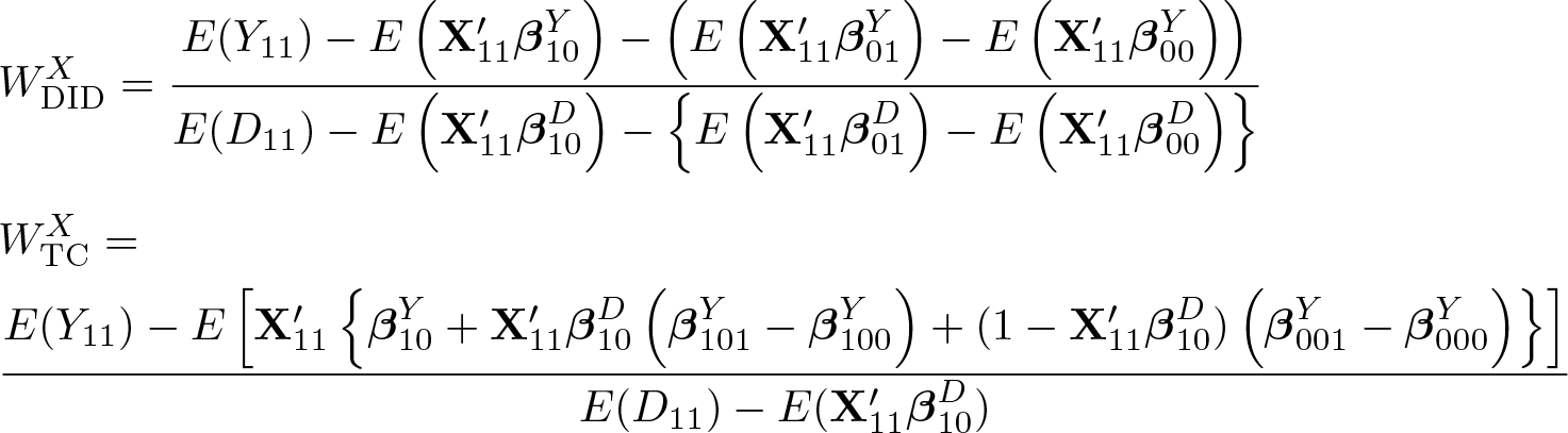
The basic setup can be extended to include covariates. Let X denote a vector of covariates, and for any random variable R, let $m_{g t}^{R} (x) = E (R_{g t} | X = x)$ . Also, let δ_d (x) = E(Y_d ₀₁|X = x) − E(Y_d ₀₀|X = x) and $\tilde{δ} (x) = E {(X_{10}) | X = x}$ . Then, define

\begin{array}{l} W_{DID}^{X} = \frac{E (Y_{11}) - E {m_{10}^{Y} (X_{11})} - E {m_{01}^{Y} (X_{11})} - E {m_{00}^{Y} (X_{11})}}{E (D_{11}) - E {m_{10}^{D} (X_{11})} - E {m_{01}^{D} (X_{11})} - E {m_{00}^{D} (X_{11})}} \\ W_{TC}^{X} = \frac{E (Y_{11}) - E {m_{10}^{Y} (X_{11}) + \tilde{δ} (X_{11})}}{E (D_{11}) - E {m_{10}^{D} (X_{11})}} \end{array}

In their article’s supplement, de Chaisemartin and D’Haultfœuille (2018b) show that $W_{DID}^{X}$ or $W_{TC}^{X}$ identifies Δ under the common support condition S(X gt) = S(X) for all (g, t) and S(X _dgt ) = S(X) for all (d, g, t) and conditional versions of assumptions 1–3 and 4–5 or 4’, respectively.⁴

Let us turn to estimators of $W_{DID}^{X}$ and $W_{TC}^{X}$ . We first consider nonparametric estimators. Let us assume that X ∈ ℝ ^r is a vector of continuous covariates. Adding discrete covariates is easy by reasoning conditional on each corresponding cell. Like for instance Frölich (2007), we first estimate conditional expectations by series estimators. For any positive integer K, let p^K (x) = {p _1K(x),…, p_KK (x)}^′ be a vector of basis functions and $P_{g t}^{K} = {p^{K} (X_{1}), . . ., p^{K} (X_{n})}$ . For any random variable R, we estimate m^R (x) = E(R|X = x) by the series estimator

{\hat{m}}^{R} (x) = p^{K_{n}} {(x)}^{'} {(P^{K_{n}} P^{K_{n'}})}^{-} P^{K_{n}} (R_{1}, . . ., R_{n})'

where (.)⁻ denotes the generalized inverse and K_n is an integer. We then estimate $m_{g t}^{R} (x) = E (R_{g t} | X = x)$ by the series estimator above on the subsample {i: G_i = g, T_i = t}. $m_{d g t}^{R} (x) = E (R_{d g t} | X = x)$ is estimated similarly. Then, our nonparametric estimators of $W_{DID}^{X}$ and $W_{TC}^{X}$ are defined as

\begin{array}{l} {\hat{W}}_{DID, NP}^{X} = \frac{\frac{1}{n_{11}} \sum_{i \in I_{11}} {Y_{i} - {\hat{m}}_{10}^{Y} (X_{i}) - {\hat{m}}_{01}^{Y} (X_{i}) + {\hat{m}}_{00}^{Y} (X_{i})}}{\frac{1}{n_{11}} \sum_{i \in I_{11}} {D_{i} - {\hat{m}}_{10}^{D} (X_{i}) - {\hat{m}}_{01}^{D} (X_{i}) + {\hat{m}}_{00}^{D} (X_{i})}} \\ {\hat{W}}_{DID, NP}^{X} = \frac{\frac{1}{n_{11}} \sum_{i \in I_{11}} [Y_{i} - {\hat{m}}_{10}^{Y} (X_{i}) - {\hat{m}}_{10}^{D} (X_{i}) {\hat{δ}}_{1} (X_{i}) - {1 - {\hat{m}}_{10}^{D} (X_{i})} {\hat{δ}}_{0} (X_{i})]}{\frac{1}{n_{11}} \sum_{i \in I_{11}} {D_{i} - {\hat{m}}_{10}^{D} (X_{i})}} \end{array}

where ${\hat{δ}}_{d} (x) = {\hat{m}}_{d 01}^{Y} (x) - {\hat{m}}_{d 00}^{Y} (x)$ . Under regularity conditions, these estimators are root-n consistent and asymptotically normal (see the supplement to de Chaisemartin and D’Haultfœuille [2018b, sec. 2.3]).

Second, we consider semiparametric estimators of $W_{DID}^{X}$ and $W_{TC}^{X}$ . For instance, assume that for $(d, g, t) \in {0, 1}^{3}, E (Y_{g t} | X) = X^{'} β_{g t}^{Y}, E (Y_{d g t} | X) = X^{'} β_{d g t}^{Y}$ , and $E (D_{g t} | X) = X^{'} β_{g t}^{D}$ . Under this assumption, we have

\begin{array}{l} W_{DID}^{X} = \frac{E (Y_{11}) - E (X_{11}^{'} β_{10}^{Y}) - (E (X_{11}^{'} β_{01}^{Y}) - E (X_{11}^{'} β_{00}^{Y}))}{E (D_{11}) - E (X_{11}^{'} β_{10}^{D}) - (E (X_{11}^{'} β_{01}^{D}) - E (X_{11}^{'} β_{00}^{D}))} \\ W_{TC}^{X} = \frac{E (Y_{11}) - E [X_{11}^{'} {β_{10}^{Y} + X_{11}^{'} β_{10}^{D} (β_{101}^{Y} - β_{100}^{Y}) + (1 - X_{11}^{'} β_{10}^{D}) (β_{001}^{Y} - β_{000}^{Y})}]}{E (D_{11}) - E (X_{11}^{'} β_{10}^{D})} \end{array}

Then, semiparametric estimators of $W_{DID}^{X}$ and $W_{TC}^{X}$ can be defined as

\begin{array}{l} W_{DID, OLS}^{X} = \frac{\sum_{i \in I_{11}} (Y_{i} - X_{i}^{'} {\hat{β}}_{10}^{Y} - X_{i}^{'} {\hat{β}}_{01}^{Y} + X_{i}^{'} {\hat{β}}_{00}^{Y})}{\sum_{i \in I_{11}} (Y_{i} - X_{i}^{'} {\hat{β}}_{10}^{D} - X_{i}^{'} {\hat{β}}_{01}^{D} + X_{i}^{'} {\hat{β}}_{00}^{D})} \\ W_{TC}^{X} = \frac{\sum_{i \in I_{11}} Y_{i} - [X_{i}^{'} {\hat{β}}_{10}^{Y} + X_{i}^{'} {X_{i}^{'} {\hat{β}}_{10}^{D} (β_{101}^{Y} - β_{100}^{Y}) + (1 - X_{11}^{'} β_{10}^{D}) (β_{001}^{Y} - β_{000}^{Y})}]}{\sum_{i \in I_{11}} (D_{i} - X_{i}^{'} {\hat{β}}_{10}^{D})} \end{array}

where for (d, g, t) ∈ {0, 1}³, ${\hat{β}}_{g t}^{Y}$ and ${\hat{β}}_{d g t}^{Y}$ denote the coefficient of X in an ordinary least-squares (OLS) regression of Y on X in the subsamples I _gt and I _dgt , respectively, and ${\hat{β}}_{g t}^{D}$ denotes the coefficient of X in an OLS regression of D on X in the subsample I _gt . When either Y or D is binary, one might prefer to posit a probit or a logit model for its conditional expectation functions in the various subsamples. Other semiparametric estimators can be defined accordingly.

Finally, researchers may sometimes wish to include a large set of controls in their estimation, which may lead to violations of the common support assumptions S(X _gt ) = S(X) and S(X _dgt ) = S(X).⁵ For instance, when the researcher wants to estimate the Wald DID, there might be values of X for which all units belong to the treatment group, thus implying that for those values, there are no control units with which the trends experienced by treatment group units can be compared. Let x ₀ denote one such problematic value; that is, x ₀ ∈ S(X ₁₁) but E(Y _0t|X = x ₀) and E(D _0t|X = x ₀) are not defined for some t ∈ {0, 1}. To avoid dropping treatment group units with X = x ₀, we use all control units to predict their counterfactual trends. Namely, in $W_{DID}^{X}$ , we replace E(Y ₀₁|X = x ₀) − E(Y ₀₀|X = x ₀) and E(D ₀₁|X = x ₀) − E(D ₀₀|X = x ₀) by E(Y ₀₁) − E(Y ₀₀) and E(D ₀₁) − E(D ₀₀). If instead the researcher wants to estimate the Wald TC, the same principle applies.

3.2 Multiple periods and groups

We now extend our initial setting to multiple periods and groups. We first define, at each period $t \in {1, . . ., \bar{t}}$ , the following “supergroup” variable:

G_{t}^{*} = 1 {E (D_{g t}) > E (D_{g t}_{- 1})} - 1 {E (D_{g t}) < E (D_{g t}_{- 1})}

Let T = t ∈ {1,…, t} : P ( $G_{t}^{*}$ = 0) > 0 denote the subset of periods t for which there exists at least one group with stable treatment rate between t − 1 and t. We let S = T{D(T ) ≠ D(T − 1), T ∈ T } denote the population of units switching between T − 1 and T ∈ T and define Δ in this setup as Δ = E{Y (1) − Y (0)|S}. For any random variable R and any (d, g, t) ∈ {0, 1} × {−1, 1} × T , we also define the following quantities:

\begin{array}{l} {DID}_{R}^{*} (g, t) = E (R | G_{t}^{*} = g, T = t) - E (R | G_{t}^{*} = g, T = t - 1) - {E (R | G_{t}^{*} = 0, T = t) - E (R | G_{t}^{*} = 0, T = t - 1)} \\ δ_{d t}^{*} = E (Y | D = d, G_{t}^{*} = 0, T = t) - E (Y | D = d, G_{t}^{*} = 0, T = t - 1) \\ Q_{d t}^{*} (y) = F_{Y | D = d, G_{t}^{*} = 0, T = t}^{- 1} \circ F_{Y | D = d, G_{t}^{*} = 0, T = t - 1} (y) \\ W_{DID}^{*} (g, t) = \frac{{DID}_{Y}^{*} (g, t)}{{DID}_{D}^{*} (g, t)} \\ W_{TC}^{*} (g, t) = \frac{E (Y | G_{t}^{*} = g, T = t) - E (Y + δ_{D t}^{*} | G_{t}^{*} = g, T = t - 1)}{E (D | G_{t}^{*} = g, T = t) - E (D | G_{t}^{*} = g, T = t - 1)} \\ W_{CIC}^{*} (g, t) = \frac{E (Y | G_{t}^{*} = g, T = t) - E {Q_{D t}^{*} (Y) | G_{t}^{*} = g, T = t - 1}}{E (D | G_{t}^{*} = g, T = t) - E (D | G_{t}^{*} = g, T = t - 1)} \end{array}

When $P (G_{t}^{*} = g) = 0$ , the three ratios above are not defined. Then, we simply let $W_{DID}^{*} (g, t) = W_{TC}^{*} (g, t) = W_{CIC}^{*} (g, t) = 0$ .

Let us then introduce the following weights,

\begin{array}{l} w_{t} = \frac{{DID}_{D}^{*} (1, t) P (G_{t}^{*} = 1, T = t) - {DID}_{D}^{*} (- 1, t) P (G_{t}^{*} = - 1, T = t)}{\sum_{t = 1}^{\bar{t}} {DID}_{D}^{*} (1, t) P (G_{t}^{*} = 1, T = t) - {DID}_{D}^{*} (- 1, t) P (G_{t}^{*} = - 1, T = t)} \\ w_{10 | t} = \frac{{DID}_{D}^{*} (1, t) P (G_{t}^{*} = 1, T = t)}{{DID}_{D}^{*} (1, t) P (G_{t}^{*} = 1, T = t) - {DID}_{D}^{*} (- 1, t) P (G_{t}^{*} = - 1, T = t)} \end{array}

where again we set ${DID}_{D}^{*} (g, t) = 0$ when P ( $G_{t}^{*}$ = g) = 0. The extensions of the Wald DID, Wald TC, and Wald CIC to multiple groups and periods are defined as

\begin{array}{l} W_{DID}^{*} (g, t) = \sum_{t \in T} w_{t} {w_{10 | t} W_{DID}^{*} (1, t) + (1 - w_{10 | t}) W_{DID}^{*} (- 1, t)} \\ W_{TC}^{*} (g, t) = \sum_{t \in T} w_{t} {w_{10 | t} W_{TC}^{*} (1, t) + (1 - w_{10 | t}) W_{TC}^{*} (- 1, t)} \\ W_{CIC}^{*} (g, t) = \sum_{t \in T} w_{t} {w_{10 | t} W_{CIC}^{*} (1, t) + (1 - w_{10 | t}) W_{CIC}^{*} (- 1, t)} \end{array}

Finally, we consider the following assumption, which replaces assumption 2.

Assumption 8. Existence of “stable” groups and independence between groups and time

T \neq \emptyset, S (D | G_{t}^{*} \neq 0, T = t - 1) \subset S (D | G_{t}^{*} = 0, T = t - 1) for all t \in T, and G ⫫ T .

Theorem 2 below shows that under our previous conditions plus assumption 8, the three estimands point identify Δ. This theorem is proved for the Wald DID and Wald TC in de Chaisemartin and D’Haultfœuille (2018a) and can be proved along the same lines for the Wald CIC.⁶

Theorem 2. Suppose that assumptions 3 and 8 hold.

If assumptions 4 and 5 are satisfied, $W_{DID}^{*} = Δ$ .

If assumption 4’ is satisfied, $W_{TC}^{*} = Δ$ .

If assumptions 6 and 7 are satisfied, $W_{CIC}^{*} = Δ$ .

To estimate $W_{DID}^{*}$ , $W_{TC}^{*}$ , and $W_{CIC}^{*}$ , we suppose that the ${(G_{t}^{*})}_{t = 1... \bar{t}}$ are known. This is the case in applications where the treatment is constant at the group × period level, as is the case in the example we revisit in section 5. When the ${(G_{t}^{*})}_{t = 1... \bar{t}}$ are unknown, it is also possible to estimate them consistently without affecting the asymptotic distribution of the estimators of $W_{DID}^{*}$ , $W_{TC}^{*}$ , and $W_{CIC}^{*}$ . We refer to section 2.1 in de Chaisemartin and D’Haultfœuille’s (2018b) supplement for details.

Let us focus on the estimator of $W_{DID}^{*}$ . The estimators of $W_{TC}^{*}$ and $W_{CIC}^{*}$ are constructed following exactly the same logic. For any random variable R and any (g, t) ∈ {−1, 0, 1} × T , let

{\hat{DID}}_{R}^{*} (g, t) = \frac{1}{n_{g t, t}^{*}} \sum_{i \in I_{g t, t}^{*}} R_{i} - \frac{1}{n_{g t, t - 1}^{*}} \sum_{i \in I_{g t, t - 1}^{*}} R_{i} - (\frac{1}{n_{0 t, t}^{*}} \sum_{i \in I_{0 t, t}^{*}} R_{i} - \frac{1}{n_{0 t, t - 1}^{*}} \sum_{i \in I_{0 t, t - 1}^{*}} R_{i})

where I _g ^∗ _t,t ′ = {i : G ^∗ _ti = g, T_i = t ^′} and n_g ^∗ _t,t ′ is the size of $I_{{_{g}}_{t, t'}}^{*}$ . We let, for $g \in {- 1, 0, 1}, \hat{P} (G_{t}^{*} = g, T = t) = n_{g t, t}^{*} / n$ . We estimate w_t and w _10|t by

\begin{array}{l} {\hat{w}}_{t} = \frac{{\hat{DID}}_{D}^{*} (1, t) \hat{P} (G_{t}^{*} = 1, T = t) - {\hat{DID}}_{D}^{*} (1, t) \hat{P} (G_{t}^{*} = - 1, T = t)}{\sum_{t = 1}^{\bar{t}} {\hat{DID}}_{D}^{*} (1, t) \hat{P} (G_{t}^{*} = 1, T = t) - {\hat{DID}}_{D}^{*} (1, t) \hat{P} (G_{t}^{*} = - 1, T = t)} \\ {\hat{w}}_{10 | t} = \frac{{\hat{DID}}_{D}^{*} (1, t) \hat{P} (G_{t}^{*} = 1, T = t)}{{\hat{DID}}_{D}^{*} (1, t) \hat{P} (G_{t}^{*} = 1, T = t) - {\hat{DID}}_{D}^{*} (1, t) \hat{P} (G_{t}^{*} = - 1, T = t)} \end{array}

We then estimate ${\hat{W}}_{DID}^{*} (g, t) by {\hat{W}}_{DID}^{*} (g, t) = {\hat{DID}}_{Y}^{*} (g, t) / {\hat{DID}}_{D}^{*} (g, t)$ , and we let

{\hat{W}}_{DID}^{*} = \sum_{t \in T} {\hat{w}}_{t} {{\hat{w}}_{10 | t} {\hat{W}}_{DID}^{*} (1, t) + (1 - {\hat{w}}_{10 | t}) {\hat{W}}_{DID}^{*} (- 1, t)}

3.3 Other extensions

We now briefly review some other extensions, for which more details can be found in de Chaisemartin and D’Haultfœuille (2018b) and its supplement.

Special cases

When P (D ₀₀ = d) = P (D ₀₁ = d) = 0 for d ∈ {0, 1}, W _TC, W _CIC, and τ _CIC,q are not defined, because δ_d and Q_d are not defined, respectively. In such cases, we can simply suppose that δ ₀ = δ ₁ and Q ₀ = Q ₁, respectively, and modify the estimators accordingly. Then the Wald TC becomes equal to the Wald DID, while the modified CIC estimands identify Δ and τ_q under the same assumptions as above and if $h_{0} {h_{0}^{- 1} (y, 1), 0} = h_{1} {h_{1}^{- 1} (y, 1), 0}$ for every y ∈ S(Y ).

No “stable” control group

In some applications (see, for example, Enikolopov, Petrova, and Zhuravskaya [2011]), the treatment rate increases in all groups, thus violating assumption 2. Then, we can still express the Wald DID as a linear combination of the LATEs of treatment and control group switchers. Specifically, let S ^′ = {D(0) ≠ D(1), G = 0} be the control group switchers and Δ^′ = E{Y (1)−Y (0)|S ^′ , T = 1} be their LATE. Under assumptions 1, 3, 4, and 5, we have

W_{DID} = α Δ + (1 - α) Δ^{'}

where α = {E(D ₁₁) − E(D ₁₀)}/[E(D ₁₁) − E(D ₁₀) − {E(D ₀₁) − E(D ₀₀)}]. Hence, the Wald DID identifies a weighted sum of Δ and Δ^′. Note, however, that if the treatment rate increases in the control group, E(D ₀₁) > E(D ₀₀) and α > 1, so Δ^′ enters with a negative weight. In this case, we may have Δ > 0 and Δ^′ > 0 and yet W _DID < 0. We will have only W _DID = Δ if Δ = Δ^′.

We can also bound Δ under assumption 4’ if assumption 2 fails. We refer to de Chaisemartin and D’Haultfœuille (2018b) for such bounds and to de Chaisemartin and D’Haultfœuille’s (2018b) supplement for their corresponding estimators.

Nonbinary treatment

The Wald DID, Wald TC, and Wald CIC still identify a causal parameter if D is not binary but is ordered and takes a finite number of values, as shown in de Chaisemartin and D’Haultfœuille (2018b). When the treatment takes many values, its support may differ in the treatment and control groups, and there may be values of D in the treatment group for which δ_d or Q_d are not defined because no unit in the control group has that value of D. This situation particularly includes the special cases discussed above. We can then slightly modify W _TC and W _CIC. Namely, let us consider a recategorized treatment $\tilde{D} = h (D)$ grouping together some values of D, and let

{\tilde{δ}}_{\tilde{d}} = E (Y_{01} | \tilde{D} = \tilde{d}) - E (Y_{00} | \tilde{D} = \tilde{d})

We then replace $δ_{D_{01}}$ by ${\tilde{δ}}_{{\tilde{D}}_{01}}$ in the definition of W _TC. Then, W _TC still identifies Δ provided that d ↦ E{Y ₁₁(d) − Y ₁₀(d)|D(0) = d} depends only on h(d). The same applies to W _CIC by using $\tilde{D}$ instead of D in Q_d (.). Using this recategorized treatment also avoids estimating δ_d and Q_d on a small number of units, thus often lowering the standard errors of the estimators.

Finally, there may also be instances where the treatment has the same support in the treatment and in the control groups but where bootstrap samples do not satisfy this requirement. For such bootstrap samples, W _TC and W _CIC cannot be estimated, and the fuzzydid command therefore sets them to 10¹⁵ or −10¹⁵ with probability 1/2. To avoid distorting inference, these bootstrap samples are not discarded in the computation of the percentile-bootstrap confidence intervals, thus enlarging these intervals.⁷ This situation is likely to arise when the treatment takes many values. Here again, it may be useful to recategorize the treatment to avoid this issue.

4 The fuzzydid command

The fuzzydid command is compatible with Stata 13.1 and later versions. It uses the moremata command (Jann 2005) to compute estimators with covariates. If this command is not already installed, one must type ssc install moremata in Stata’s command line.

4.1 Syntax

The syntax of fuzzydid is as follows:

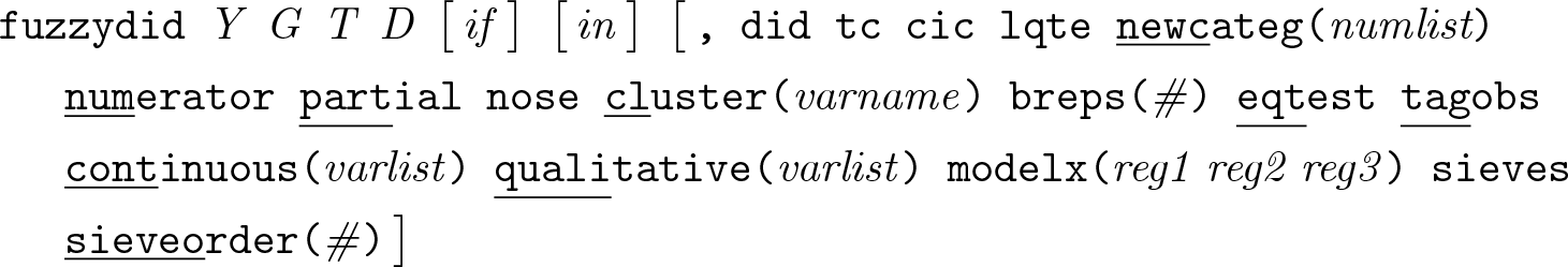
Y is the outcome variable.

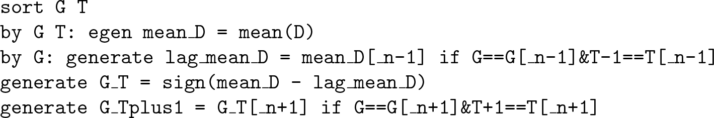
G is the group variable or variables. When the data bear only two groups and two periods, G merely corresponds to the variable G defined in section 2, an indicator for units in the treatment group. Outside of this special case, G should list the variables $G_{t}^{*}$ and $G_{t + 1}^{*}$ defined in section 3.2. Below are some lines of code that users can follow to create these two variables:

Sometimes, there may not be groups where the treatment is perfectly stable between consecutive periods, thus implying that the Wald DID, Wald TC, and Wald CIC estimators cannot be computed with the G_T and G_Tplus1 variables defined above. The user may then replace the fourth line of code above with

where ε is a positive number small enough to consider that the mean treatment did not really change in groups where it changed by less than ε. See section 2.1 in de Chaisemartin and D’Haultfœuille’s (2018b) supplement for one possible method to choose ε.

T is the time-period variable with values in {0,…, t}.

D is the treatment variable. It can be any ordered variable.

4.2 Description

fuzzydid estimates Δ or τ_q using one or several of the estimators defined in sections 2 and 3 above. It also computes their standard errors and confidence intervals.

4.3 Options

General options

did computes ${\hat{W}}_{DID}$ if no covariates are included in the estimation. If some covariates are included, it computes ${\hat{W}}_{DID,NP}^{X}$ , ${\hat{W}}_{DID,OLS}^{X}$ , or another estimator with covariates depending on the options specified by the user.

tc computes ${\hat{W}}_{TC}$ if no covariates are included in the estimation. If D is binary and P (D ₀₀ = 0) = P (D ₀₁ = 0) ∈ {0, 1}, the command actually computes ${\hat{W}}_{DID}$ , following the discussion in section 3.3. If some covariates are included, it computes ${\hat{W}}_{TC,NP}^{X}$ , ${\hat{W}}_{TC,OLS}^{X}$ , or another estimator with covariates depending on the options specified by the user.

cic computes ${\hat{W}}_{CIC}$ . If D is binary and P (D ₀₀ = 0) = P (D ₀₁ = 0) ∈ {0, 1}, the command actually computes ${\tilde{W}}_{CIC}$ , following the discussion in section 3.3. This option can be specified only when no covariates are included in the estimation.

lqte computes ${\hat{τ}}_{q}$ , for q ∈ {0.05, 0.10,…, 0.95}. This option can be specified only when D, G, and T are binary and no covariates are included in the estimation. When P (D ₀₀ = 0) = P (D ₀₁ = 0) ∈ {0, 1}, the command computes ${\hat{τ}}_{q_{,}_{CIC}}$ , following the discussion in section 3.3.

At least one of the four options above is required. If several of these options are specified, the command computes all the estimators requested by the user.

newcateg( numlist ) groups some values of the treatment together when estimating δ_d and Q_d . This option may be useful when the treatment takes many values, as explained in section 3.3. One must specify the upper bound of each set of values of the treatment one wants to group. For instance, if D takes the values {0, 1, 2, 3, 4.5, 7, 8}, and one wants to group together units with D = {0, 1, 2}, {3, 4.5}, and {7, 8} when estimating δ_d and Q_d , one must write newcateg(2 4.5 8).

numerator computes only the numerators of the ${\hat{W}}_{DID}$ , ${\hat{W}}_{TC}$ , and ${\hat{W}}_{CIC}$ estimators. As explained in section 3.3.3 in de Chaisemartin and D’Haultfœuille (2018b), this option is useful to conduct placebo tests of the assumptions underlying each estimator.

partial computes the bounds of Δ defined in section 3.3, ${\underline{\hat{W}}}_{TC}$ and ${\hat{\bar{W}}}_{TC}$ . This option can be specified only when no covariates are included in the estimation.

nose computes only the estimators, not their standard errors.

cluster( varname ) computes the standard errors of the estimators using a block bootstrap at the varname level. Only one clustering variable is allowed.

breps( # ) specifies the number of bootstrap replications. The default is breps(50).

eqtest performs an equality test between the estimands when the user specifies at least two of the did, tc, and cic options.

tagobs creates a new variable named tagobs, which identifies the observations used by fuzzydid.

Options specific to estimators with covariates

continuous( varlist ) specifies the names of all the continuous covariates that must be included in the estimation.

qualitative( varlist ) specifies the names of all the qualitative covariates that must be included in the estimation. For each variable, indicator variables are created for each value except one and included as controls in the estimation.

modelx( reg1 reg2 reg3 ) specifies which parametric method should be used to estimate the conditional expectations in $W_{DID}^{X}$ or $W_{TC}^{X}$ . reg1 specifies which method should be used to estimate E(Y_gt |X) and E(Y_dgt |X). reg2 specifies which method should be used to estimate E(D_gt |X). When D is not binary, reg3 specifies which method should be used to estimate ${P (D_{g t} = d | X)}_{d}_{\in {1, ..., \bar{d}}}$ . The possible methods are ols, logit, and probit. For instance, if the user writes modelx(ols logit logit), the command estimates E(Y_gt |X) and E(Y_dgt |X) by OLS and E(D_gt |X) and ${P (D_{g t} = d | X)}_{d}_{\in {1, ..., \bar{d}}}$ by a logistic regression. The logit and probit options can be used only with binary variables.

sieves indicates that the conditional expectations in $W_{DID}^{X}$ and $W_{TC}^{X}$ should be estimated nonparametrically (see section 3.1 above).

When covariates are included in the estimation, and neither modelx() nor sieves is specified, the command estimates by default all conditional expectations by OLS.

sieveorder( # ) specifies the order of the sieve basis when the option sieves is used. It must be greater than or equal to 2. For a given order L, the number of basis functions is given by $(\begin{matrix} p_{c} + L \\ L \end{matrix})$ , where p_c is the number of continuous covariates. The command does not allow for more than min(4800, n/5) basis functions, where n is the number of observations. By default, the choice of the sieve order is done via fivefold cross-validation with a mean squared error loss function.

4.4 Stored results

fuzzydid stores the following in e():

e(N), a scalar containing the number of observations used in the estimation.

If the user specifies at least one of the did, tc, and cic options, fuzzydid saves e(b_LATE), a k × 1 matrix, where k is equal to the number of options specified. The lines of the matrix correspond to each of the requested estimators. If nose is not specified, fuzzydid also saves e(se_LATE) and e(ci_LATE), which are a k × 1 and a k × 2 matrix, respectively. The lines of e(se_LATE) correspond to the bootstrap standard error associated with each of the requested estimators. The columns of e(ci_LATE) store the lower and upper bounds, respectively, of the 95% confidence interval computed by percentile bootstrap for each requested estimator.

If the user specifies the eqtest option and at least two of the did, tc, and cic options, fuzzydid saves three matrices e(b_LATE_eqtest), e(se_LATE_eqtest), and e(ci_LATE_eqtest). The first two matrices have dimension $(\begin{matrix} k \\ 2 \end{matrix}) \times 1$ while the third has dimension $(\begin{matrix} k \\ 2 \end{matrix}) \times 2$ , where k is equal to the number of the did, tc, and cic options specified. The matrices e(b_LATE_eqtest) and e(se_LATE_eqtest) store the value of the difference between each pair of estimators and the associated bootstrap standard error, respectively. The columns of e(ci_LATE_eqtest) store the lower and upper bounds, respectively, of the 95% confidence interval computed by percentile bootstrap associated with each difference.

If the user specifies the lqte option, the command saves e(b_LQTE), a 19 × 1 matrix. The lines of the matrix store the value of ${\hat{τ}}_{q}$ for q ∈ {0.05, 0.10,…, 0.95}. If nose is not specified, fuzzydid also saves e(se_LQTE) and e(ci_LQTE), a 19×1 and a 19 × 2 matrix, respectively. The lines of e(se_LQTE) correspond to the bootstrap standard error associated with ${\hat{τ}}_{q}$ for q ∈ {0.05, 0.10,…, 0.95}. The columns of e(ci_LQTE) store the lower and upper bounds, respectively, of the 95% confidence interval computed by percentile bootstrap for each of the 19 LQTE estimators.

5 Example

To illustrate the use of fuzzydid, we rely on the same dataset as Gentzkow, Shapiro, and Sinkinson (2011) to study the effect of newspapers on electoral participation.

turnout_dailies_1868-1928.dta is a county-level dataset. It contains two variables of interest, pres_turnout and numdailies, that represent the turnout (Y ) and the number of newspapers available (D), respectively, in each U.S. county and at each presidential election from 1868 to 1928. First, we load the dataset and present summary statistics:

The average turnout in the 1868 to 1928 presidential elections across counties is 65.01%. The number of newspapers ranges from 0 to 45 and is on average equal to 1.46.

Second, we use fuzzydid to compute ${\hat{W}}_{DID}^{*}$ , ${\hat{W}}_{TC}^{*}$ , and ${\hat{W}}_{CIC}^{*}$ using the first two time periods in the dataset, the 1868 and 1872 elections. We then define the G1872 variable, which is equal to 1 or 0 in counties whose number of newspapers increased or remained stable, respectively, between the 1868 and 1872 elections. For now, counties where that number decreased are excluded from the analysis. numdailies takes many values, so there are values taken by counties with G1872 = 1 that are not taken by any county with G1872 = 0. Therefore, we use newcateg() to recategorize numdailies into four categories: zero, one, two, and three or more newspapers.⁸ Finally, we cluster the bootstrap at the county level to allow for county-level correlation over time.

The columns of the output table show, respectively, the value of each estimator, its bootstrap standard error, its t statistic, its p-value, and the lower and upper bounds of its 95% confidence interval. All point estimates are positive, but none are statistically significant, presumably because this restricted sample with two time periods is too small. In this simple example with two periods and no controls, the computation of the estimators and of 200 bootstrap replications takes only about 3 seconds on a Dell Optiplex 9020 with an Intel Core i7-4790 CPU 3.60 GHz processor and 16 GB of RAM, using Stata/MP with 4 cores.

Third, we compute estimators of the LQTEs, again using the 1868 and 1872 elections. We use a binary treatment variable numdailies_bin (0 newspaper, 1 or more) because LQTEs can be estimated only with a binary treatment.

To preserve space, we report only ${\hat{τ}}_{0.2}$ , ${\hat{τ}}_{0.4}$ , ${\hat{τ}}_{0.6}$ , and ${\hat{τ}}_{0.8}$ , but the command computes ${\hat{τ}}_{q}$ for q ∈ {0.05, 0.10,…, 0.95}. ${\hat{τ}}_{0.4}$ is negative, while the other estimates are positive, thus suggesting that numdailies_bin may have heterogeneous effects along the distribution of the outcome. However, none of the point estimates are statistically significant.

Fourth, we compute ${\hat{W}}_{DID}^{*}$ , ${\hat{W}}_{TC}^{*}$ , and ${\hat{W}}_{CIC}^{*}$ on the full sample. For that purpose, we define the G_T and G_Tplus1 variables described in section 4.2. G_T is equal to 1, 0, or −1 for county c × election-year t observations such that the number of newspapers increased, remained stable, or decreased, respectively, between election-years t − 1 and t in that county. G_Tplus1 is the lead of G_T. We add the eqtest option to test whether the estimators are significantly different.

The Wald DID is equal to 0.0038. According to that estimator, increasing the number of newspapers available in a county by one increases voters’ turnout in presidential elections by 0.38 percentage points. This estimator is significantly different from 0 at the 5% level. The Wald TC is larger (0.0053) and significantly different from the Wald DID (t statistic = −4.51). The Wald CIC lies in between (0.0042), and this estimator is not significantly different from the other two. In this more complicated example with 16 periods and almost 17,000 observations, computing the estimators and 200 bootstrap replications still takes only around two minutes.

Gentzkow, Shapiro, and Sinkinson (2011) allow for state-specific trends in their specification, so we compute ${\hat{W}}_{DID}^{*}$ and ${\hat{W}}_{TC}^{*}$ with state indicators as controls, which is equivalent to allowing for state-specific trends.⁹

With those controls, ${\hat{W}}_{DID}^{*}$ = 0.0026 and ${\hat{W}}_{TC}^{*}$ = 0.0043, and the two estimators are significantly different at the 10% level (t statistic = −1.85). Adding the control variables substantially increases the computation time to 79 minutes.

Finally, we compute a placebo Wald DID or Wald TC estimator to assess if assumptions 4 and 5 or assumption 4’, respectively, is plausible in this application. Instead of using the turnout in county g and election-year t as the outcome variable, our placebo estimators use the turnout in the same county in the previous election. Moreover, only counties where the number of newspapers did not change between t − 2 and t − 1 are included in the estimation. Therefore, our placebo estimators compare the evolution of turnout from t−2 to t−1, between counties where the number of newspapers increased or decreased between t − 1 and t and counties where that number remained stable, restricting the sample to counties where the number of newspapers remained stable from t − 2 to t − 1.

The placebo Wald DID is negative, indicating that the actual Wald DID may be downward biased because of a violation of assumptions 4 and 5. However, this placebo estimator is not statistically significant. The placebo Wald TC is also negative and not statistically significant. It is twice smaller than the placebo Wald DID, thus indicating that assumption 4’ may be more plausible than assumptions 4 and 5 in this application.

6 Monte Carlo simulations

This section exhibits the finite sample performance of the estimators of W _DID, W _TC, W _CIC, and τ _CIC,q. For that purpose, we consider the following data-generating process (DGP). Let (G, T ) be uniform on {0, 1}². Let {U(0), U(1), V } ∼ N (0, Σ), with Σ _ii = 1 for i ∈ {1, 3}, Σ₂₂ = 1.2, Σ₁₂ = 0, Σ₁₃ = 0.5, and Σ₂₃ = −0.5 and with {U(0), U(1), V }⫫(G, T ). Then, we let

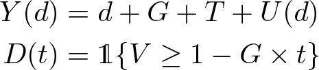
\begin{array}{l} Y (d) = d + G + T + U (d) \\ D (t) = 1 {V \geq 1 - G \times t} \end{array}

In this DGP, all the assumptions in section 2 hold. Therefore, W _DID, W _TC, and W _CIC all identify Δ, while τ _CIC,q identifies τ_q . We focus on the bias, mean square error, and coverage rate of estimators of Δ and τ_q for q ∈ {0.25, 0.5, 0.75} and for sample sizes equal to 400, 800, and 1,600. In this DGP, Δ ≃ 0.540, τ _0.25 ≃ 0.481, τ _0.5 ≃ 0.536, and τ _0.75 ≃ 0.595.

The results are displayed in table 1. Even with small samples, the Wald DID and Wald TC estimators do not exhibit any systematic bias. Their root mean squared errors (RMSE) are also similar. The Wald CIC, conversely, is more biased and has an RMSE that is 5 to 15% larger. This is probably due to the estimator of the nonlinear transform Q_d . This estimator is likely biased and imprecise in the tails, which may also explain the bias and high RMSE of ${\hat{τ}}_{q}$ for n = 400. Note, however, that the bias of ${\hat{W}}_{CIC}$ , ${\hat{τ}}_{0.25}$ , ${\hat{τ}}_{0.5}$ , and ${\hat{τ}}_{0.75}$ decreases quickly with the sample size. For n = 1600, the bias of these estimators is already negligible compared with their RMSE. Finally, the percentile bootstrap confidence intervals of all estimators are quite accurate, with all coverage rates lying between 0.92 and 0.97 when the nominal level is 0.95. The levels are slightly more distorted for the Wald CIC and the ${\hat{τ}}_{q}$ , but again, they become closer to 95% as the sample size increases.

Table 1.

Results of the Monte Carlo simulations

		Estimators of Δ			Estimators of ${\hat{τ}}_{q}$
n	Statistic	${\hat{W}}_{DID}$	${\hat{W}}_{TC}$	${\hat{W}}_{CIC}$	${\hat{τ}}_{0.25}$	${\hat{τ}}_{0.5}$	${\hat{τ}}_{0.75}$
400	Bias	0.005	−0.002	0.174	0.002	−0.154	−0.497
	RMSE	0.651	0.613	0.682	0.712	0.867	1.223
	Cov. rate	0.948	0.948	0.921	0.971	0.967	0.917
800	Bias	0.015	0.01	0.088	−0.056	−0.029	−0.235
	RMSE	0.422	0.414	0.472	0.539	0.555	0.922
	Cov. rate	0.953	0.951	0.929	0.964	0.961	0.934
1600	Bias	−0.005	−0.005	0.034	−0.054	−0.013	−0.077
	RMSE	0.286	0.284	0.329	0.394	0.382	0.58
	Cov. rate	0.948	0.946	0.943	0.964	0.966	0.955

NOTES: “Cov. rate” stands for coverage rates of (percentile bootstrap) confidence intervals, with a nominal level of 95%. The results are based on 1,000 samples, and for each, 500 bootstrap samples are drawn to construct the confidence intervals. With our DGP, Δ ≃ 0.540, τ _0.25 ≃ 0.481, τ _0.5 ≃ 0.536, and τ _0.75 ≃ 0.595.

7 Conclusion

We have discussed how to use fuzzydid to estimate LATE and LQTE in fuzzy DID designs, following de Chaisemartin and D’Haultfœuille (2018b). In such designs, the popular Wald DID estimand relies on a stable treatment-effect assumption, which may not be plausible. Then, the Wald TC and Wald CIC estimands may be valuable alternatives because they do not hinge upon this assumption. Similarly, when the data bear multiple groups and periods, the Wald TC and Wald CIC estimands may be valuable alternatives to commonly used two-way linear regressions. The fuzzydid command makes it easy to estimate those estimands.

Supplemental Material

Supplemental Material, st0560 - Fuzzy differences-in-differences with Stata

Supplemental Material, st0560 for Fuzzy differences-in-differences with Stata by Clément de Chaisemartin, Xavier D’Haultfœuille and Yannick Guyonvarch in The Stata Journal

Footnotes

Notes

References

Athey

Imbens

G. W.

2006. Identification and inference in nonlinear differencein-differences models. Econometrica 74: 431–497.

Chernozhukov

Fernández-Val

Galichon

2010. Quantile and probability curves without crossing. Econometrica 78: 1093–1125.

de Chaisemartin

D’Haultfœuille

2018a. Two-way fixed effects estimators with heterogeneous treatment effects. ArXiv Working Paper No. arXiv:1510.01757. https://arxiv.org/abs/1803.08807.

de Chaisemartin

D’Haultfœuille

2018b. Fuzzy differences-in-difference. Review of Economic Studies 85: 999–1028.

Enikolopov

Petrova

Zhuravskaya

2011. Media and political persuasion: Evidence from Russia. American Economic Review 101: 3253–3285.

Frölich

2007. Nonparametric IV estimation of local average treatment effects with covariates. Journal of Econometrics 139: 35–75.

Gentzkow

Shapiro

J. M.

Sinkinson

2011. The effect of newspaper entry and exit on electoral politics. American Economic Review 101: 2980–3018.

Jann

2005. moremata: Stata module (Mata) to provide various functions. Statistical Software Components S455001, Department of Economics, Boston College. https://ideas.repec.org/c/boc/bocode/s455001.html.

Supplementary Material

Please find the following supplemental material available below.

For Open Access articles published under a Creative Commons License, all supplemental material carries the same license as the article it is associated with.

For non-Open Access articles published, all supplemental material carries a non-exclusive license, and permission requests for re-use of supplemental material or any part of supplemental material shall be sent directly to the copyright owner as specified in the copyright notice associated with the article.

2.18 MB

0.00 MB