
Abstract
The different discrete transform techniques such as discrete cosine transform (DCT), discrete sine transform (DST), discrete wavelet transform (DWT), and mel-scale frequency cepstral coefficients (MFCCs) are powerful feature extraction techniques. This article presents a proposed computer-aided diagnosis (CAD) system for extracting the most effective and significant features of Alzheimer’s disease (AD) using these different discrete transform techniques and MFCC techniques. Linear support vector machine has been used as a classifier in this article. Experimental results conclude that the proposed CAD system using MFCC technique for AD recognition has a great improvement for the system performance with small number of significant extracted features, as compared with the CAD system based on DCT, DST, DWT, and the hybrid combination methods of the different transform techniques.
Keywords
Introduction
Alzheimer’s disease (AD) is the most common type of dementia, which is defined as “a collection of symptoms that include reduction in intellectual functioning such as thinking, remembering, and reasoning.” Alzheimer’s disease is a progressive disease, which means that it gets worse over time. 1,2 There is no cure, specific blood, or imaging test for AD. However, some drugs are available that may help slow the progression of Alzheimer’s symptoms for a limited time. Diagnosis of the AD still a challenge and difficult, especially in the early stages. An early diagnosis helps individuals receive treatment for symptoms and delay the development of AD. 3
Brain function images, such as magnetic resonance imaging (MRI), positron emission tomography (PET), and single photon emission computed tomography (SPECT), have been proved to be very effective in this task. 3 -6 Several CAD systems based on medical imaging are developed to allow detection of the AD at early stages by comparing normal and diseased participants using the analysis of certain features in brain images. The analysis of images can be done using several methods. One of the important method is the statistical parametric mapping (SPM) software that models data of individual voxel. 7,8 Other method for the analysis of structural MRI images is executed by voxel-based morphometry (VBM). 9,10
Different approaches were used for developing CAD systems for early diagnosis of the AD using MRI brain images. 11,12 In the study by Mahanand et al, 11 the features had been extracted using VBM with a self-adaptive resource allocation network classifier for the diagnosis of AD for MRI images. Principal component analysis (PCA) has been used for feature reduction. A total of 30 patients and 30 normal persons used for this study from the Open Access Series of Imaging Studies (OASIS) database. In the study by Mahmood and Ghimire, 12 the PCA had been used. Next, a multiclass neural network is used to classify the reduced dimensions from PCA. Two hundred and thirty diagnosed MRI images obtained from the OASIS MRI database are used for training the neural network, and then the trained neural network tested with 457 MRI images.
There are other approaches for early diagnosis of AD presented in the study by Chaves et al and Martinez-Murcia et al, 13,14 where they used another type of brain images database of SPECT and PET. In the study by Chaves et al, 13 an association rule (AR) mining had been used for early diagnosis of AD using voxel selection method using the SPECT and PET databases. The ARs had been used for dimensionality reduction, PCA and partial least squares had been used as feature extraction techniques, and support vector machine (SVM) had been used as a classifier. In the study by Martinez-Murcia et al, 14 a CAD system divided into 3 stages had been used for early diagnosis of AD using the SPECT and PET databases. These stages are voxel selection, feature extraction, and classification. Mann–Whitney–Wilcoxon U test is used for voxel selection. Then, feature reduction step is done using factor analysis by extracting common factors from the selected voxels. The last stage is using a linear SVM classifier.
There are different approaches that uses different discrete transform techniques with MRI brain images as presented in the study by Patil and Yardi 15 , Gouid et al, 16 and Herrera et al 17 In the study by Patil and Yardi, 15 the discrete cosine transform (DCT) coefficients had been used as input features for the neural network classification. The features had been used to train a neural network to automatically classify MRI image whether it is normal brain or brain with AD. In the study by Gouid et al, 16 the brain tumors had been extracted using the SVM classifier to distinguish the tumor from MRI images of the brain. A database of 20 MRI images including normal and abnormal tumors had been used in this study. In the study by Herrera et al, 17 a methodology for classification of AD from MRI images using a large database had been presented. The wavelet feature extraction from the MRI had been used as a dimensionality reduction step, and then SVM classifier had been used.
In this article, a new approach based on extracting significant features of 3-dimensional (3D) MRI images from the OASIS 18,19 data set is proposed. The proposed approach depends on extracting different features from MRI images using different discrete transforms such as DCT, discrete sine transform (DST), and discrete wavelet transform (DWT). Mel-scale frequency cepstral coefficients (MFCCs) technique is also used for extracting the significant features from MRI images after converting the 3D images to 1-dimensional (1D) signal. A comparison is done between the algorithm given by Dessouky et al 20 with the features extracted from DCT, DST, DWT, and MFCC. The results clearly indicate that better performance achieved by the proposed approach based on extracting features using MFCC technique rather than the proposed approaches based on the other different discrete transform techniques will be presented in this article.
The rest of this article is organized as follows: the second section introduces the used database. The third section discusses the proposed AD recognition system using different discrete transform techniques such as DCT, DST and DWT, and MFCC and Hybrid methods. The fourth section introduces the performance evaluation metric parameters. The fifth section presents the experimental results, discussion, and analysis. Result discussion given in the sixth section, and the conclusion is presented in the last section.
Neuroimaging Materials and Data Set
The database that has been used for this study is the OASIS. 18,19 The OASIS database used to determine the sequence of events that happened in the progression of AD. The database consists of a cross-sectional collection of 416 participants aged between 33 and 96 years. The participants include normal individuals who has no disease (no dementia) with Clinical Dementia Rating (CDR) of 0, participants who have been diagnosed with very mild AD (CDR = 0.5), participants with mild AD (CDR = 1), and participants with moderate AD (CDR = 2).
The participants include both men and women. More women than men have AD and other dementias. Almost two-thirds of Alzheimer’s are women. Based on estimates from Aging, Demographics, and Memory Study (ADAMS), among people aged 71 years and older, 16% of women have AD and other dementias compared with 11% of men. The reason why more women than men have AD is the fact that women live longer than men on average, and older age is the greatest risk factor for AD. It is also found that there is no significant difference between men and women in the proportion who develop AD or other dementias at any given age. 1
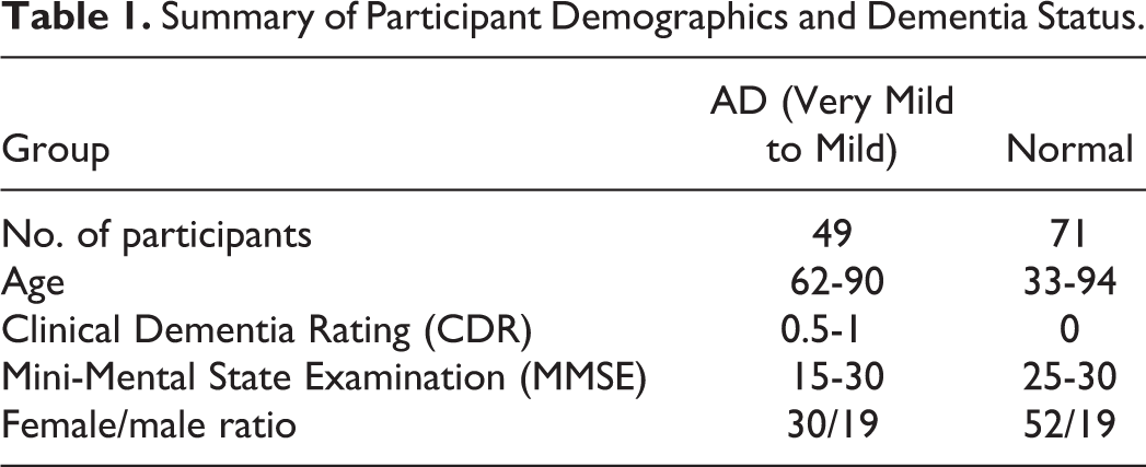
In this study, T1-weighted magnetic resonance volumes of 49 patients having AD diagnosed with “very mild AD to mild AD” and 71 normal participants are used. All participants underwent 3D and MRI scans. The participants were randomly chosen to cover a wide and different ranges of age and Mini-Mental State Examination. The females are more than males because females are more susceptible to AD than males because they are older as denoted earlier. Table 1 summarizes important clinical and demographic information for each group.
Summary of Participant Demographics and Dementia Status.
The Proposed Recognition System
The proposed AD recognition system indicated in Figure 1 consists of 6 stages. These stages are summarized as follows:
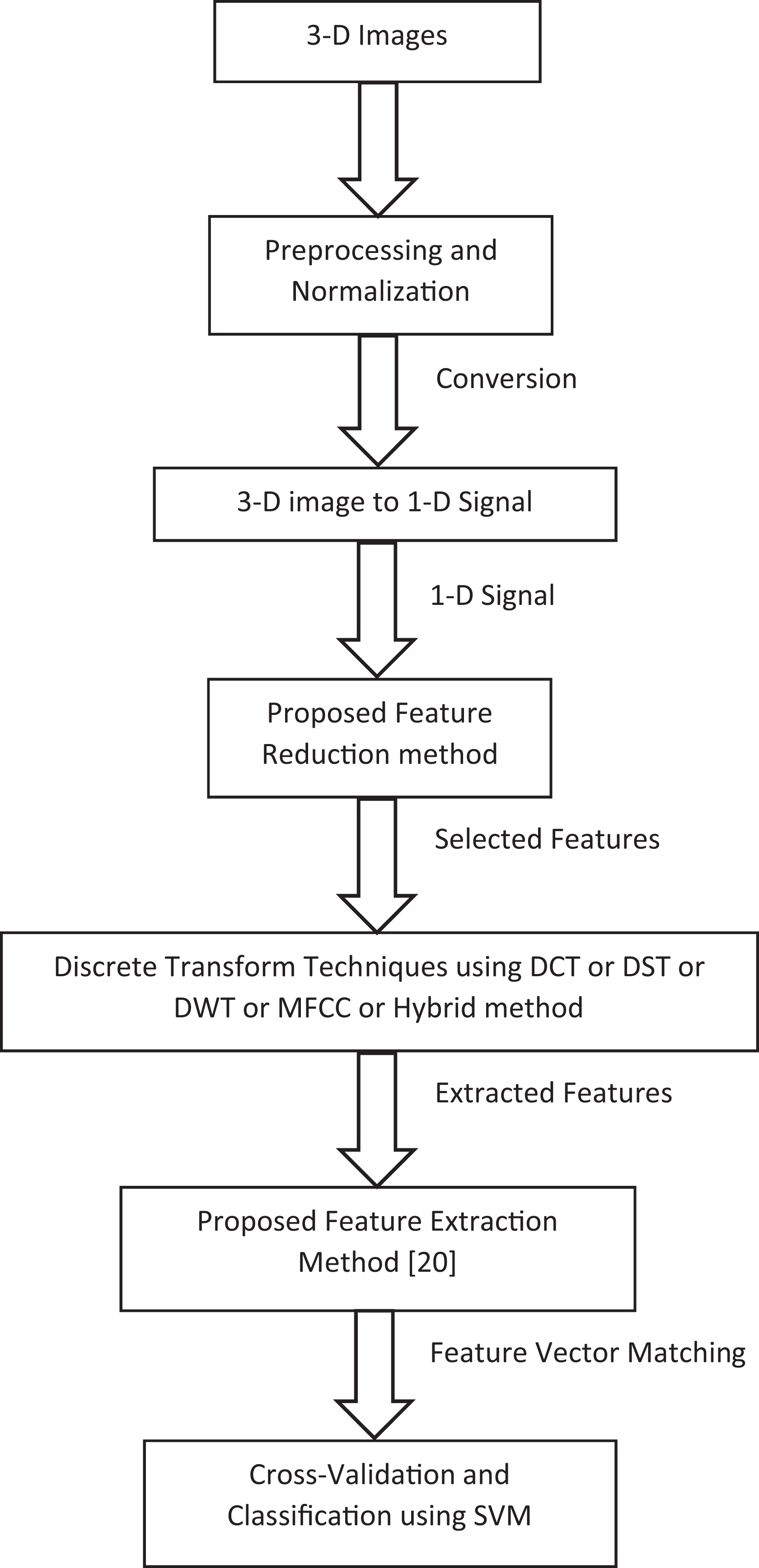
The proposed Alzheimer’s disease recognition system.
Preprocessing and normalization of the images, converting the 3D image to 1D signal, apply the proposed feature selection method, apply different discrete transform techniques such as DCT, DST, DWT, or MFCC technique or hybrid of different techniques, apply the proposed feature extraction method,
20
perform the cross-validation, and classification process using SVM classifier.
Preprocessing and Normalization
The 3D structural MRI images must be first preprocessed and normalized using the SPM. 7,8 The analysis of structural MRI images is executed by VBM. 9,10 Voxel-based morphometry is suitable for large-scale cross-sectional MRI images. Voxel-based morphometry is a voxel-wise comparison of the regional differences in gray matter (GM) among groups of participants using MRI scans. The steps of VBM are spatial normalization, segmentation, smoothing, and statistical analysis. Spatial normalization depends on making registration to all the brain MRI images with respect to a common template. Next, the registered images are then segmented into 3 classes: GM, white matter, and cerebrospinal fluid. In the next step, segmented GM images are then smoothed by convolving them with 10 mm full-width at half-maximum isotropic Gaussian kernel. Finally, in the statistical analysis part, a 2-sample t test is performed on the smoothed GM images of normal persons and patients with AD. 7,9
In this study, only the first step (spatial normalization) of the VBM was used. It is not needed to segment the images as this study is done on all brain images, neither the smoothing nor statistical analysis is done not to change the brain images. The dimensionality of the images before preprocessing was 6 44 3008 (176 × 208 × 176) pixels, and after preprocessing and normalization step, the dimensions of the images reduced to 2 12 2954 (121 × 145 × 121) pixels. For more details, see the study by Dessouky et al. 20
Three-Dimensional Images Conversion to 1D Signals
The 3D images converted to 1D signal using reshape MatLab function, which is defined as following 21 :

The output B is an n-dimensional array with the same elements as A, but reshaped to size (SIZ), a vector representing the dimensions of the reshaped array. The whole images are converted not separated into x, y, or z axis. 21
After conversion, each image is presented as a 1D vector. Each image has a 2 12 2954 pixel. These 1D signals are applied as input to the next steps.
Proposed Feature Reduction Approach
The images matrix was reconstructed for 120 images, each one has 2 12 2945 pixels in 1 row. This is a very large dimensionality for each image, which needs very large memory size and more time to select the effective features. The proposed feature reduction method depends on reducing the dimensionality of each image. This method based on removing the pixels in the same place with the same intensity (gray) level from all images and keep the other pixels. This step is more important and efficient, where the dimensionality of each image reduces from 2 12 2945 pixels per image to only 6 90 432 pixels per image. The dimensionality of each image is reduced by about 33%. This will save the memory and make the feature extraction faster and more efficient. In addition to mathematical computational statistical techniques, feature extraction can be performed heuristically by picking such features from a pattern vector that could be assumed to be useful in classification.
Feature Extraction Techniques
Significant features can be extracted from the images using different discrete transform techniques such as DCT, DST, and DWT. There is also the MFCCs technique that can also be used to extract the significant features.
Discrete cosine transform
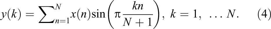
Discrete cosine transform has been highly used in image processing and signal analysis due to its “energy compaction” property. It compresses most signal information in some coefficients. Considering this, DCT is chosen for feature extraction. Discrete cosine transform is applied on entire brain image, which results in low and high frequency coefficient feature matrix of same dimensions. The most commonly used DCT equation that returns the unitary DCT of x 15 :
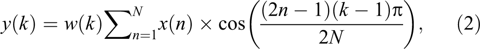
where x (n) is the input vector for each image, N is the number of features in each image, and w (k) is defined as following:
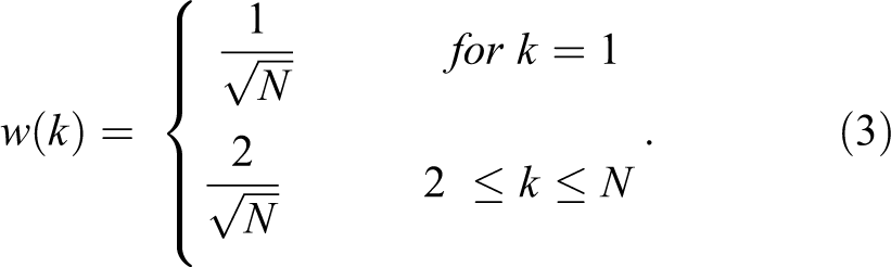
Here, N is the length of x, k = 1, 2, 3 … N features, and x (n) and y (k) are of the same size.
Discrete Sine Transform
The DST looks like the discrete Fourier transform (DFT), but it uses a real matrix. It is equal to twice the length of the DFT’s imaginary parts, working on real data where the Fourier transform is imaginary for a real part and odd for odd function. The DST matrix is formed by arranging these sequences row wise. Mathematically, the DST is represented by 22 :
Discrete Wavelet Transform
The main reasons for using the DWT lie in its complete theoretical framework, the great flexibility for choosing bases, and the low computational complexity. The data are decomposed into different frequency components by wavelets, and then each component is matched to its scale. Although the Fourier Transform only represents the images based on its frequency component, so it loses time information of the signal, and the wavelets are local in both frequency and time and are able to analyze data at different scales or resolutions much better than sine transform and cosine transform. 17
The DWT depends on passing a signal (x) through a series of filters. First, passing the samples through a low-pass filter, which has impulse response of (g), the convolution results of the 223:

The high-pass filter decomposes the signal simultaneously. The detail coefficients are outputted from the high-pass filter, and the approximation coefficients are outputted from the low-pass filter. The output of the filter is decomposed into 2 parts (g: high pass and h: low pass) 23 :


Mel-Frequency Cepstral Coefficients
Mel-scale frequency cepstral coefficients are derived through cepstral analysis, which are used for extracting the significant features from the signal. The MFCC features are also based on the human perception of frequency content that emphasizes low-frequency components more than high-frequency components. The MFCC feature extraction steps can be summarized as follows
24
-26
: perform the Fourier transform of the signal with a sampling rate equal to 11 025 Hz, map the powers of the spectrum using triangular overlapping windows, apply the log of power at each of the Mel frequency, perform DCT of the Mel log power just as a signal, the MFCCs are amplitudes of resulting spectrum, select the effective number of cepstral coefficients, and calculate the number of filters in filter bank.
Figure 2 depicts the block diagram steps of the MFCC process. To calculate the MFCC based on 1D signal, the input images must be first converted from 3D to 1D signal. 24
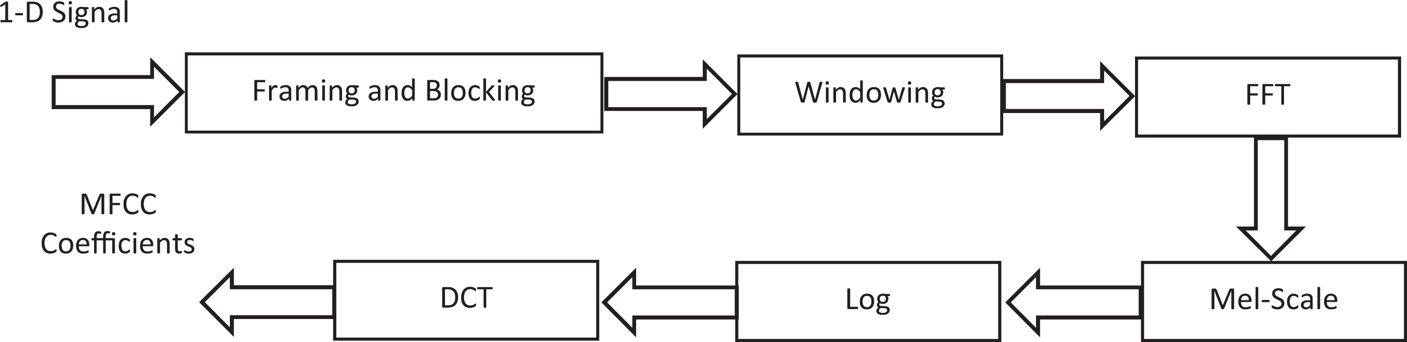
Mel-scale frequency cepstral coefficient (MFCC) process of 1D AD signal. Abbreviation: FFT, Fast Fourier Transform.
The input signal blocked into N samples of frames. The frame overlapping is used to prevent information loss. The first frame consists of the first N samples. This process continues until all are accommodated within one or more frames.
Windowing step is applied to each individual frame to raise the continuity between neighbor frames and to minimize the signal discontinuities at the beginning and at the end of each frame and minimizing the spectral distortion. Common windowing functions include the rectangular window, Hamming window, triangular window, Blackman window, and flattop window. The most commonly used window function is Hamming window computed from the equation 24 -26 :
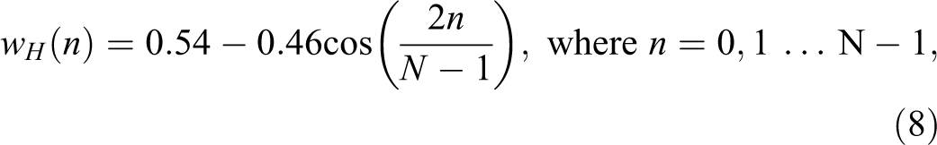
where wH (n) is the defined window, N stands for the quantity of samples within every frame.
In the next step, the Fast Fourier Transform (FFT) of windowed frames of 1D signal of AD images is computed, which converts each frame from time domain s(n) to frequency domain S(k). In this process, each frame is converted to N samples from time domain to frequency domain using the FFT. The FFT can be calculated as 24 -26 :

Next, the spectrum is frequency wrapped to transform the spectrum to mel-frequency scale. The mel-frequency wrapping is done by a mel-filter bank composed of a set of filters with constant bandwidths. The bank has 1 filter for each mel-frequency component, and each filter consists of a triangular filter frequency response. The triangular filters are in the range from 0 to the Nyquist frequency. The number of filters parameter affects the accuracy of the system. In this article, the number of filters in filter bank equals to 24 :

where (Fb) is the number of filter bank and (Sr) is the sampling rate and equal to 11 025 Hz. The mel is a unit to measure the frequency of the tone, and the mel-scale is a connection between the real frequency scale (Hz) and the frequency scale (mel). Mel-scale is calculated as 24 -26 :
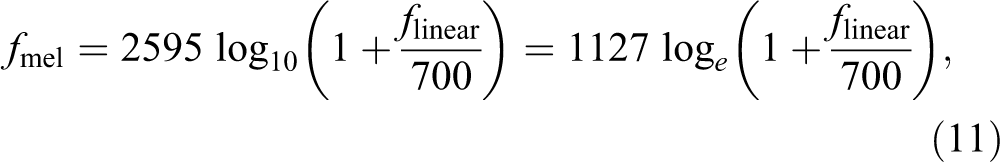
where f linear is the actual frequency in Hz. The log mel-frequency spectrum is converted back to time domain using the DCT.
For this transformation, the DFT or DCT can be used for calculating the coefficients. But, DFT is used for spectral analysis and DCT used for data compression, and DCT signals have more information concentrated in a small number of coefficients. So, it is easy with lower storage for representing mel spectrum in a small number of coefficients. The output after applying DCT is MFCCs 24 :
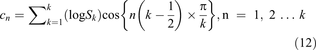
where Sk , K = 1, 2 … K are the outputs of the last step. If the energy of the mth mel-filter output is S(m), the MFCCs will be 24 :
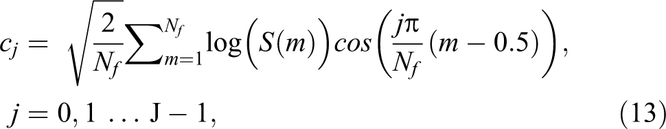
where j is the number of MFCCs, Nf is the number of mel-filters, and cj are the MFCCs.
Proposed Feature Extraction Algorithm Steps
In this section, most significant features are needed to be extracted from the features of DCT, DST, DWT, or MFCC to reduce the high dimensionality of each image. Ignoring unnecessary features is important to make the comparison between demented and non-demented participants more easy, reduce the high dimensionality of each image, and increase the accuracy of the classifier without discarding any important information. The proposed feature extraction algorithm is summarized in the following steps: Step 1: Dividing the participants into 2 different classes, the first class includes the images of participants with dementia (patient) and the other class contains the images of nondemented participants (normal). Step 2: Calculating the mean for each feature in each class, where µ1 is the mean of the first class and µ2 is the mean of the second class. µ1 will be a matrix of 1 × 6 90 432 features and µ2 will be also 1 × 6 90 432 features.
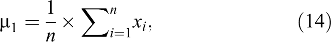
where n is the number of images in the first class and xi represents each image in this class. µ1 is repeated for each feature in the first class, that is, µ1 is repeated 6 90 432.
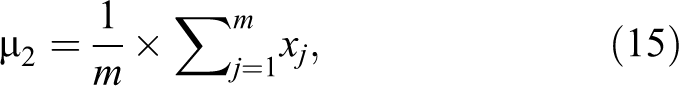
where m is the number of images in the second class and xj
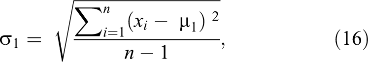
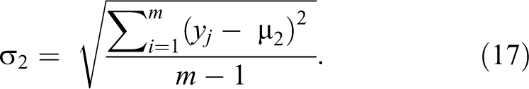
represents each image in this class. µ2 is repeated for each feature in the first class, that is, µ2 is repeated 6 90 432. Step 3: Calculate standard deviation for each feature in each class, where σ1
will be a matrix of 1 × 6 90 432 features and σ2
will be also 1 × 6 90 432 features.
Step 4: Maximize the difference between the means of the 2 classes by making absolute difference between the means of the each feature of the 2 classes and divide the result by the multiplication of the standard deviation of each feature of the 2 classes.
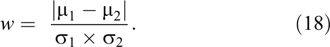
So, w is the maximum difference between the 2 classes, µ1 and µ2 are the means, and σ1 and σ2 are the standard deviations of the first and second class, respectively. Step 5: w is calculated in percentage for each feature to understand how much information each feature has.
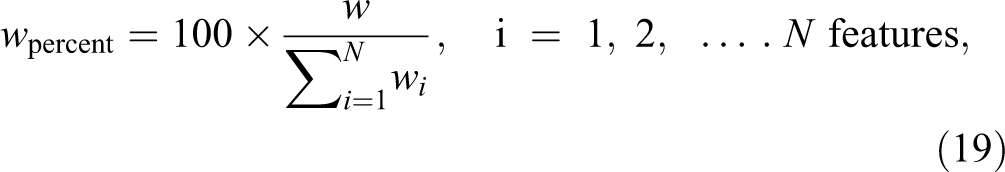
where w percent is calculated for each feature in all images, and is the summation of all features. Then, w is sorted in descending to sort the features that have high information in the first. Selecting the higher ordered features with higher information will give higher classifier performance with smaller number of features.
Cross-Validation
Cross-validation is an evaluating method that statistically compares algorithms by partitioning the data into 2 groups: the first used for learning or training a model and the second used for validating this model. The training and validation groups must successively cross-over in rounds where each data point has a chance to be validated. The k-fold cross-validation is a basic form of cross-validation. There are different cross-validation forms, which are special cases of k-fold cross-validation or used as iterative rounds of k-fold cross-validation. 27,28
In k-fold cross-validation, the data are first partitioned into k equally (or nearly equally) sized segments or folds. Subsequently, k iterations of training and validation are performed such that within each iteration, a different fold of the data is held out for validation, whereas the remaining k − 1 folds are used for learning. Figure 3 demonstrates an example with k = 3. The darker sections of the data are used for training, whereas the lighter sections are used for validation. In data mining and machine learning, 10-fold cross-validation (k = 10) is the most common. 27,28
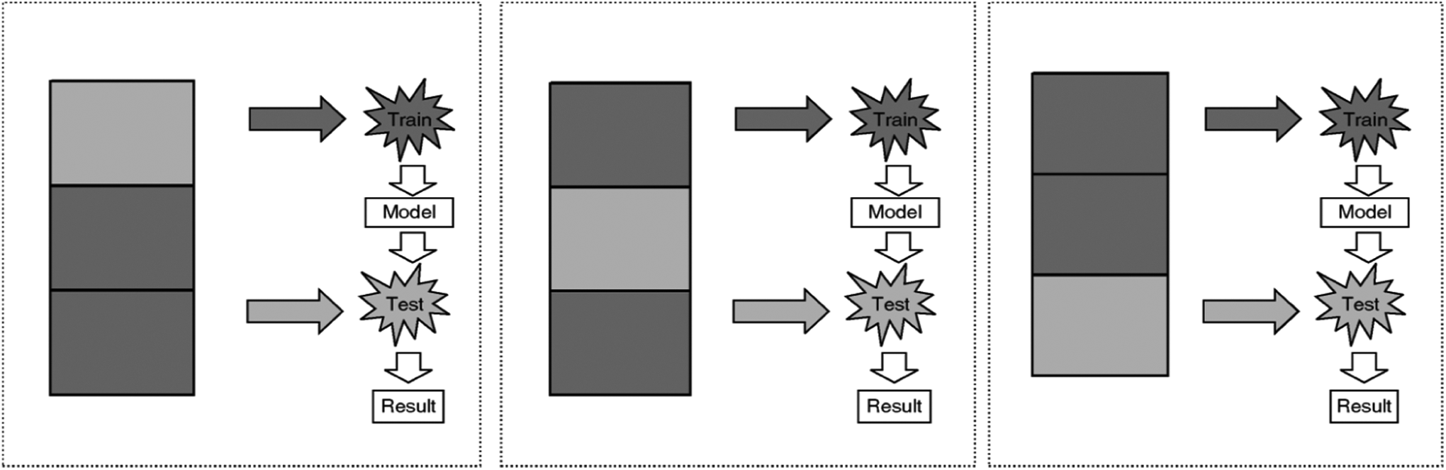
Procedure of 3-fold cross-validation.
The first appearance of the cross-validation was at 1930s in the study by Larson, 29 where only one sample is used for training and other one was used for testing. Different works tried to develop the idea as in the study by Mosteller and Turkey, 30 where the first time the cross-validation expression is used and it looks like the current k-fold cross-validation. In 1970s, cross-validation has been employed for selecting suitable parameters instead of using only cross-validation to validate the system performance as presented in the study by Geisser and Stone. 31,32 Nowadays, cross-validation is used in different applications of the data mining and machine learning for performance estimation and model selection.
There are 2 possible goals in cross-validation
27
: to estimate performance of the learned model from available data using 1 algorithm. In other words, to gauge the generalizability of an algorithm and to compare the performance of 2 or more different algorithms and find out the best algorithm for the available data or alternatively to compare the performance of 2 or more variants of a parameterized model.
The problem now is choosing the suitable value of k. Larger the k, more performance could be estimated, the size of the training set is closer to the size of data to make most of data to train the model, and the overlap between training sets also increases. If 5-fold cross-validation is used as an example, each training set will have ¾ of the data with each of the other 4 training sets, but with 10-fold cross-validation, each training set has 8/9 of the data. So, k = 10 is a good choice because it makes predictions using 90% of the data, making it more likely to be generalizable to the full data. 27
In this work, 10-fold cross-validation is used on the whole database for performance estimation. The cross-validation is done after extracting the significant feature from each image using DCT, DST, DWT, or MFCC and separating the images into training and testing sets using 10-fold cross-validation.
Support Vector Machine Classification
Support vector machine is used as a classifier, and it has gained popularity in recent years because of its superior performance in practical applications, especially in the field of bioinformatics. A 2-class SVM classifier aims to do a hyperplane that maximizes the margin, which is the distance between the closest points on either side of the boundary. These points are known as the support vectors, and their role is the construction of a maximum-margin hyperplane. 16,20,33,34
Performance Evaluation Metric Parameters
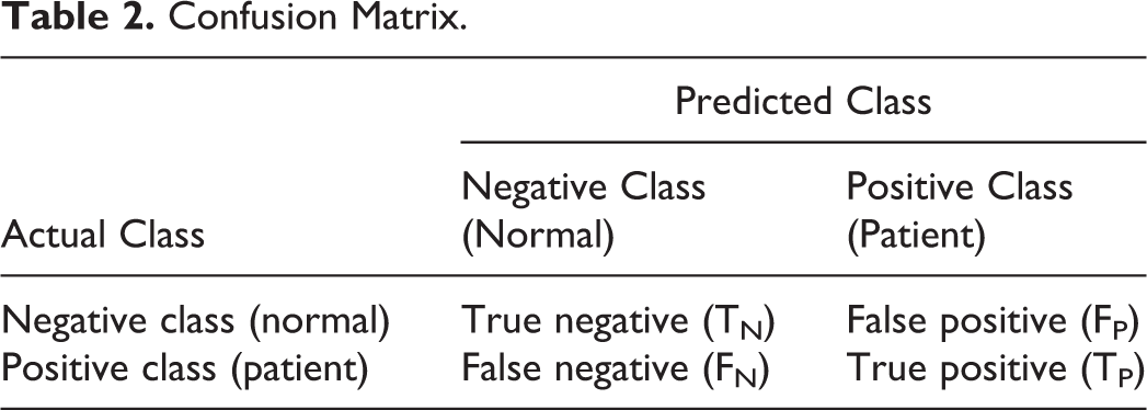
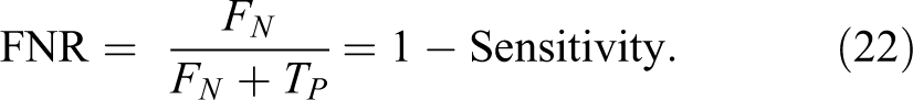
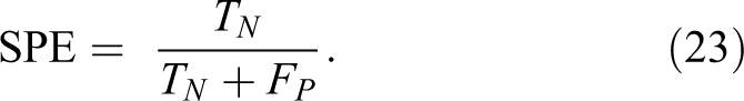
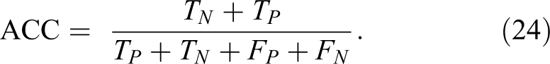
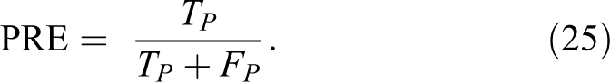
This section presents the metric parameters that will be used for measuring the performance of the proposed algorithm. The simplest measurements would be the classification accuracy rate, which is calculated from the number of correctly predicted samples divided by the total number of predicted samples. Often, a single measurement is not sufficient, especially in the cases of disease diagnosis, when the costs of classifying patients into normal and the reverse are not the same. Positive means that this person is a patient and negative means that the person is normal. To test the results, the true positive, true negative, false positive, and false negative are defined as
35,36
: true positive (TP): positive (patient) samples correctly classified as positive (patient), false positive (FP): negative (normal) samples incorrectly classified as positive (patient), true negative (TN): negative (normal) samples correctly classified as negative (normal), and false negative (FN): positive (patient) samples incorrectly classified as negative (normal).
Table 2 presents a confusion matrix of several common metrics that can be calculated from it. 35,36
Confusion Matrix.
The Proposed Algorithm Performance Evaluation Parameters
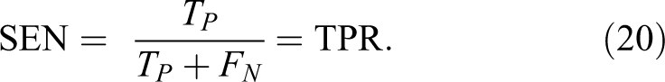
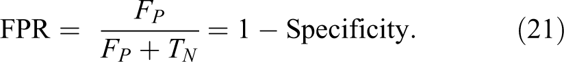
The metric parameters that will be used to measure the performance of the proposed algorithm are:
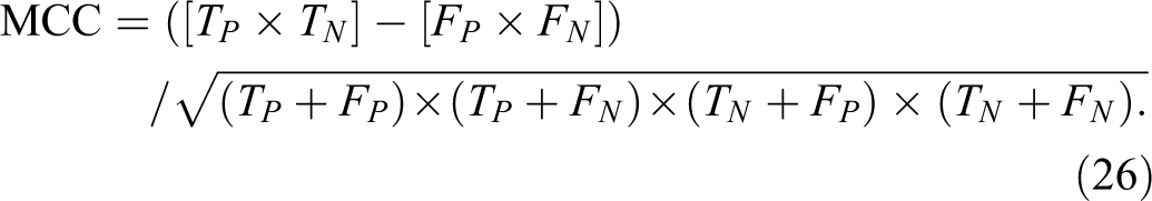
7. Matthews correlation coefficient (MCC) is calculated by 35 :
Experimental Results
This section presents the obtained results of the metric parameters used for measuring the performance of the previous algorithm given in the study by Dessouky et al, 20 the proposed approach based on MFCC technique, and the proposed approach based on different discrete transform techniques (DCT, DST, or DWT). In addition, the study includes the proposed approach based on using 2 different hybrid methods, that is, the combination between DCT and DWT and the combination between DST and DWT are also presented. The comparison study for the previous algorithm and all proposed approaches is discussed. The obtained results depict the variation of SEN, SPE, ACC, and MCC as a function of the number of extracted features.
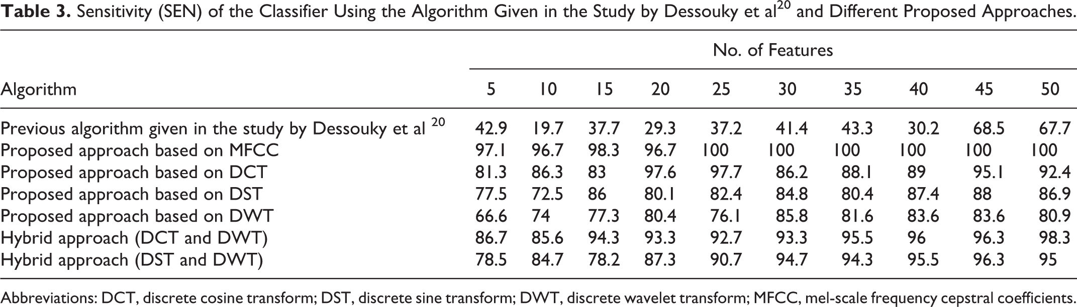
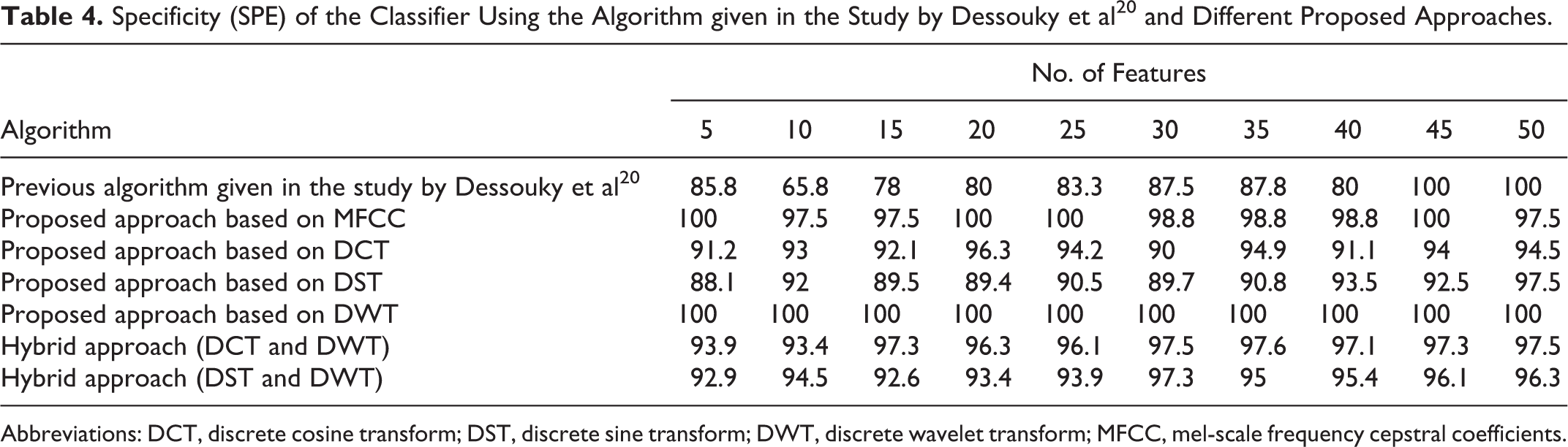
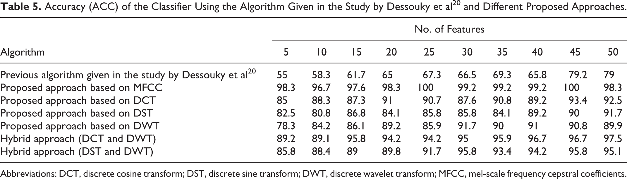
Tables 3 to 6 and Figures 4 to 7 present the obtained results for the metric parameters: SEN, SPE, ACC, and MCC of the classifier, respectively. These metric parameters are measured for the previous algorithm given in the study by Dessouky et al, 20 and all the proposed approaches are based on MFCC technique, different discrete transforms techniques, and hybrid methods. The main aim is to get high metric value with small number of features.
Sensitivity (SEN) of the Classifier Using the Algorithm Given in the Study by Dessouky et al 20 and Different Proposed Approaches.
Abbreviations: DCT, discrete cosine transform; DST, discrete sine transform; DWT, discrete wavelet transform; MFCC, mel-scale frequency cepstral coefficients.
Specificity (SPE) of the Classifier Using the Algorithm given in the Study by Dessouky et al 20 and Different Proposed Approaches.
Abbreviations: DCT, discrete cosine transform; DST, discrete sine transform; DWT, discrete wavelet transform; MFCC, mel-scale frequency cepstral coefficients.
Accuracy (ACC) of the Classifier Using the Algorithm Given in the Study by Dessouky et al 20 and Different Proposed Approaches.
Abbreviations: DCT, discrete cosine transform; DST, discrete sine transform; DWT, discrete wavelet transform; MFCC, mel-scale frequency cepstral coefficients.
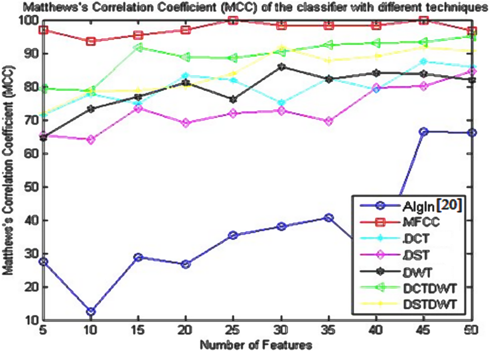
Matthews’s Correlation Coefficient (MCC) of the Classifier Using the Algorithm given in the Study by Dessouky et al 20 and Different Proposed Approaches.
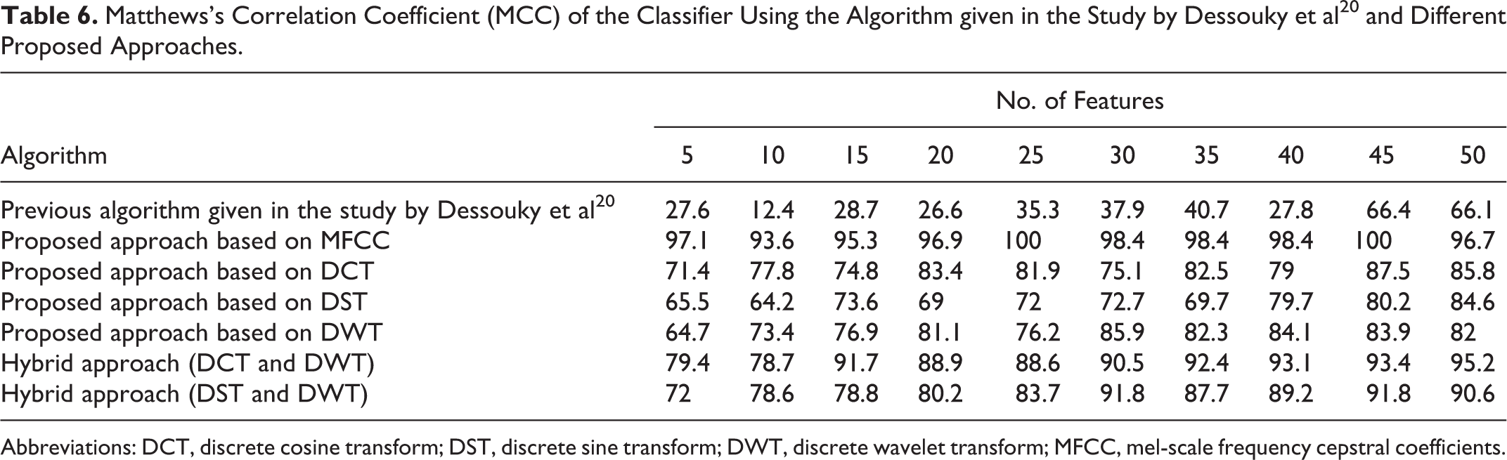
Abbreviations: DCT, discrete cosine transform; DST, discrete sine transform; DWT, discrete wavelet transform; MFCC, mel-scale frequency cepstral coefficients.
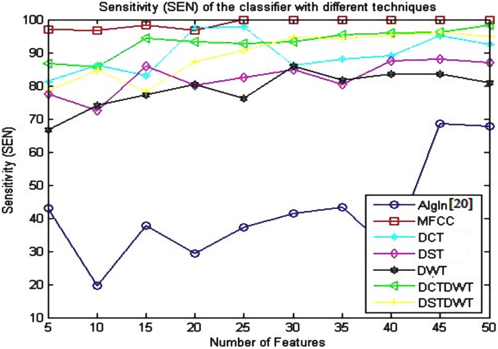
Sensitivity (SEN) of the classifier using the algorithm given in the study by Dessouky et al 20 and different proposed approaches.
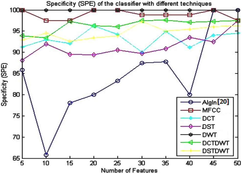
Specificity (SPE) of the classifier using the algorithm given in the study by Dessouky et al 20 and different proposed approaches.
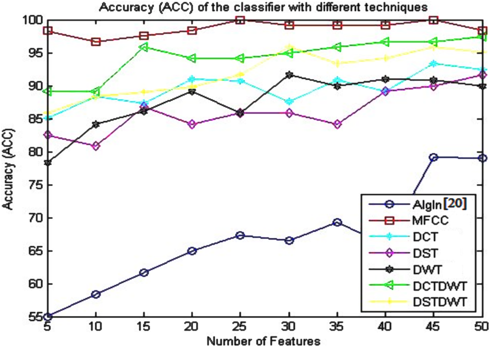
Accuracy (ACC) of the classifier using the algorithm given in the study by Dessouky et al 20 and different proposed approaches.
Matthews’s correlation coefficient (MCC) of the classifier using the algorithm given in the study by Dessouky et al 20 and different proposed approaches.
The obtained results presented in Table 3 and illustrated in Figure 4 indicate that the SEN gives the best results (100%) using proposed approach based on MFCC technique with small number of features (25 features). The SEN value remains stable at the same value with the increase in the number of features. For the other proposed approaches, the SEN didn’t reach to this value.
The presented results given in Table 4 and depicted in Figure 5 show that the SPE attends to its optimum value (100%) using the proposed approaches based on DWT and MFCC techniques as compared to the other proposed approaches. The proposed approach based on DWT gives the value of 100% for the specificity with the stability advantage that the SPE value retains at the same value as the number of features increases from 5 to 50. The proposed approach based on MFCC gives also the same value of the specificity (100%) with small number of features.
Table 5 and Figure 6 give the obtained results for the ACC metric parameter using all proposed approaches. From these results, it is seen that the ACC has better results using proposed approach based on MFCC technique as compared to the other proposed approaches. The accuracy of the classifier reaches to 100% with small number of features (25 features).
The concluded results given in Table 6 and shown in Figure 7 denote that the MCC has better results using the proposed approach based on MFCC technique as compared to the obtained results based on the other proposed approaches. The MCC of the classifier equals to 100% with small number of features (25 features).
Processing Time and Dependency Analysis
The speed of the system includes and depends on all the processing or execution time required to perform all the operation stages for the proposed algorithm. The processing time depends on the number of all operation steps performed using the proposed approaches. The execution time (T) can be calculated using the following equation:

where, t 1 is the processing time needed to perform all operation steps for the proposed feature reduction method; t 2 is the required processing time to perform the transformation techniques (DCT, DST, or DWT) or hybrid techniques (DCT + DWT, DST + DWT, or MFCC technique); t 3 is the required processing time to perform all operation steps for proposed feature extraction method given in the study by Dessouky et al 20 ; t 4 is the processing time for descending sorting the extracted features; t 5 is the processing time for evaluating the cross-validation and dividing the images into 10-folds; t 6 is the processing time for training and testing the classifier using SVM algorithm.
Table 7 presents the processing time required to realize and perform the proposed algorithm steps with different transformation techniques. These results show that the processing time has a small and a negligible difference as compared to the required time for the previous algorithm given in the study by Dessouky et al 20 and the proposed algorithm based on MFCC technique.
Execution and Processing Time for Different Transformation Techniques.
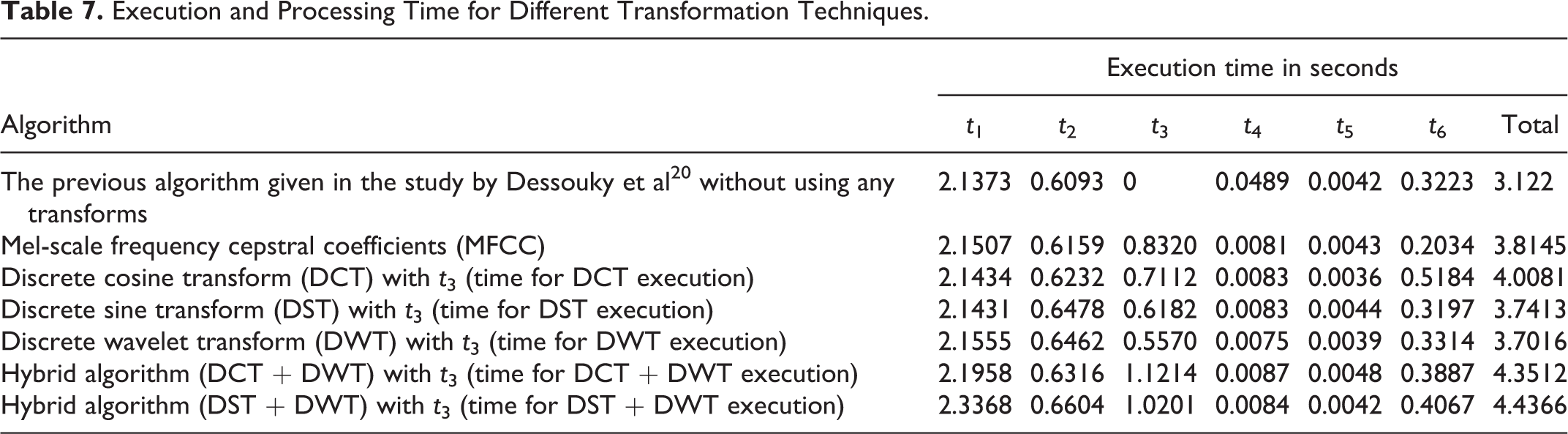
Figure 8 records how the system time is consumed by different system stages. It is noticed that more than half of the time is consumed at the first step of the preprocessing stage and proposed feature selection method stage.
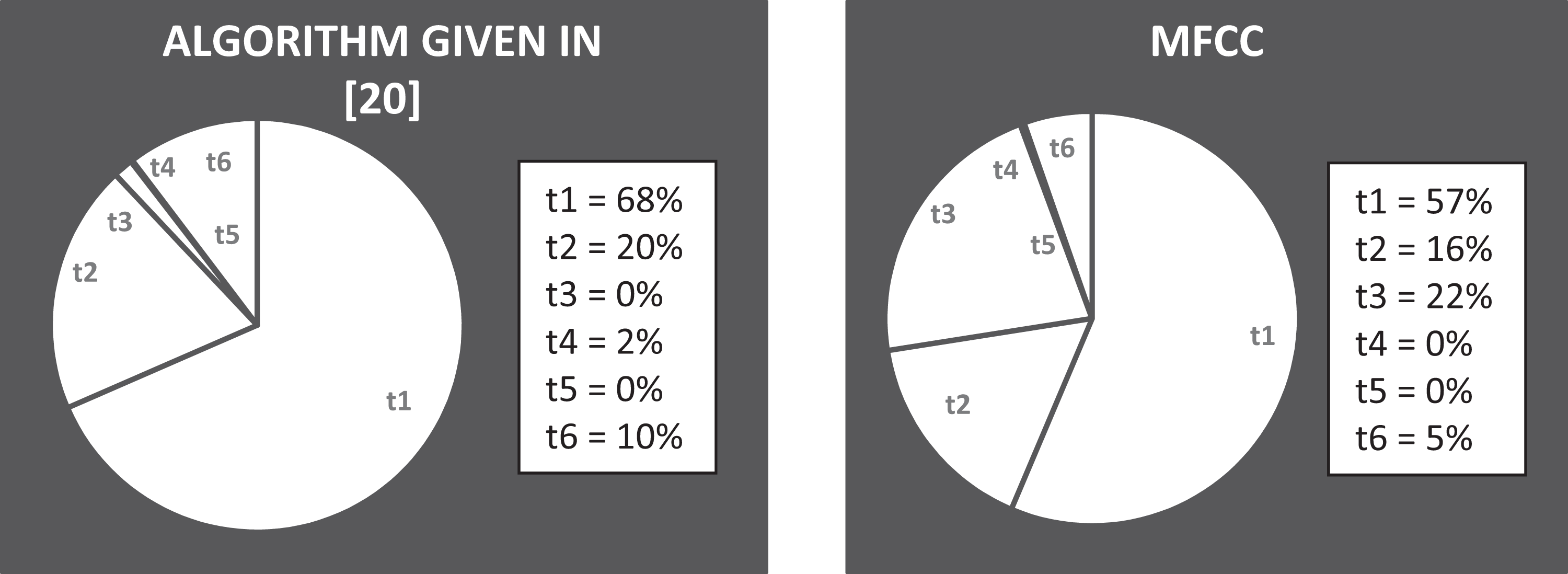
The system runtime analysis of the previous algorithm given in the study by Dessouky et al 20 and the proposed algorithm using the Mel-scale frequency cepstral coefficient (MFCC) technique.
Result Discussion
When dealing with pictorial information, the amount of data per one object can be huge. The pattern vectors have more than a million components. The most part of these data is useless for classification. In feature extraction, the features that best characterize the data are searched for best data classification. The statistical technique is used to reduce the dimensionality of the data vector while retaining most of the information that the data vector contains.
The main challenge in this article is the diagnosis of the AD at early stages with low number of extracted features, fast execution time, and memory size reduction. The perfect classifier would assign every object to the correct class, that is, the main task in this article is to design the classifier with minimum errors as possible, using small number of extracted effective features.
The results presented and given previously in the fifth section conclude that the metric parameters such as SEN, SPE, ACC, and MCC of the classifier equal 100% using smaller number of features (25 features) using the proposed approach based on MFCC technique as compared to the previous algorithm given in the study by Dessouky et al 20 and the other proposed approaches based on different discrete techniques as presented in this article. This is very significant for the memory size reduction with a negligible increase in the processing or execution time, and this consequently reduces the hardware implementation of the proposed CAD system.
The trend for the AD is to build up a CAD system to assist the medical doctors to easly diagnosis it without the need to ask about the symptoms, do physical examinations, check neurological functions, or ask for blood tests and urine samples.
Conclusion
This article presents a proposed approach and built up a CAD system for extracting the most significant feature extraction using different discrete transform techniques and MFCC technique. The metric parameters are used to measure the performance of the classifier based on MFCC technique (100%) using small number of features (25 features) as compared to the previous algorithm and the other proposed approaches based on different discrete transform techniques. This leads to reduction in the memory size. Thus, this is very useful for simplifying the hardware implementation, consequently reducing the cost, and better performance with negligible increase of the execution and processing time.
Footnotes
This article was accepted under the editorship of the former Editor-in-Chief, Carol F. Lippa.
Declaration of Conflicting Interests
The authors declared no potential conflicts of interest with respect to the research, authorship, and/or publication of this article.
Funding
The authors received no financial support for the research, authorship, and/or publication of this article.