Sage Journals: Discover world-class research

Abstract

A novel framework for the classification of lung nodules using computed tomography scans is proposed in this article. To get an accurate diagnosis of the detected lung nodules, the proposed framework integrates the following 2 groups of features: (1) appearance features modeled using the higher order Markov Gibbs random field model that has the ability to describe the spatial inhomogeneities inside the lung nodule and (2) geometric features that describe the shape geometry of the lung nodules. The novelty of this article is to accurately model the appearance of the detected lung nodules using a new developed seventh-order Markov Gibbs random field model that has the ability to model the existing spatial inhomogeneities for both small and large detected lung nodules, in addition to the integration with the extracted geometric features. Finally, a deep autoencoder classifier is fed by the above 2 feature groups to distinguish between the malignant and benign nodules. To evaluate the proposed framework, we used the publicly available data from the Lung Image Database Consortium. We used a total of 727 nodules that were collected from 467 patients. The proposed system demonstrates the promise to be a valuable tool for the detection of lung cancer evidenced by achieving a nodule classification accuracy of 91.20%.

Keywords

computer-aided diagnosis higher order MGRF computed tomography autoencoder pulmonary nodule lung cancer

Introduction

Lung cancer is the second most common cancer in men and women all over the world. It comes after prostate cancer in men and after breast cancer in women. Moreover, it is considered the leading cause of cancer-related death among both genders in the United States, as the number of people who die each year of lung cancer is more than the number of people who die of breast and prostate cancers combined.¹ The number of patients suffering from lung cancer has recently increased significantly all over the world, which increases the motivation in developing accurate and fast diagnostic tools to detect lung cancer earlier in order to increase the patients’ survival rate. Lung nodules are the first indication to start diagnosing lung cancer. It can be benign (normal subjects) or malignant (cancerous subjects). Figure 1 shows some samples of benign and malignant lung nodules. Histological examination using biopsies is considered the gold standard for the final diagnosis of pulmonary nodules. Even though resection of pulmonary nodules is the ideal and reliable way for diagnosis, there is a crucial need for developing a noninvasive diagnostic tool to eliminate the risks associated with the surgical procedure.

Figure 1.

Sample 2D axial projection for benign (first row) and malignant (second row) lung nodules.

In general, there are several imaging modalities used to diagnose the pulmonary nodules, such as chest radiography (X-ray), magnetic resonance imaging (MRI), positron emission tomography (PET) scan, and computed tomography (CT) scans. Some researchers prefer the use of MRI to avoid ionizing radiation exposure.² Diffusion-weighted MRI has been reported to be used for lung cancer diagnosis, as it could be used to qualitatively check the high b-value images and apparent diffusion coefficient (ADC) maps in addition to quantitatively generating the mean and median tumor ADCs.³ However, CT and PET scans are the most widely used modalities for diagnosis and staging of lung cancer. A CT scan is more likely to clearly show lung tumors than other modalities because of its high resolution and clear contrast compared with other modalities. We will focus and utilize the CT scans in our study as it is considered a routine procedure for patients who have lung cancer in addition to its ability to provide high-resolution pulmonary anatomical details.

Recently, a lot of researchers tried to develop computer-aided diagnostic (CAD) systems to classify pulmonary nodules to earlier detect lung cancer. In particular, Thamilselvan and Sathiaseelan⁴ implemented an enhanced k nearest neighbor (EKNN) technique to identify the lung cancer through the automatic classification of benign and malignant tissues. In their system, they improved the quality of images using morphological methods. Then, an EKNN classifier has been used for the identification of the cancer and classification of the images. They implemented 4 steps of k nearest neighbor that were calculated based on Euclidean distance to permit them to do the classification, define the k value, assign majority class, and find the minimum distance. Lee et al ⁵ proposed a lung nodule classification system using a random forest (RF) classifier aided by clustering. After they merged all the data, they divided it into 2 clusters, then divided each cluster into 2 groups, nodule and nonnodule. Finally, a RF classifier was trained for each cluster to distinguish between benign and malignant nodules. They used chest CT scans for 332 patients including 5721 images. They got a sensitivity of 98.33% and a specificity of 97.11% for their proposed system. Sun et al ⁶ used deep learning algorithms for benign/malignant classification on the Lung Image Database Consortium (LIDC) data set. After rotating and downsampling, they collected 174 412 samples with 52 × 52 pixel each and the corresponding ground truth. They designed and implemented 3 deep learning algorithms named Deep Belief Networks (DBNs), Convolutional Neural Network (CNN), and Stacked Denoising Autoencoder (SDAE). The performance of deep learning algorithms was compared with traditional CAD systems by designing a scheme with 28 image features and support vector machine (SVM) classifier. The accuracies of CNN, SDAE, and DBNs were 0.79, 0.79, and 0.81, respectively; the accuracy of their designed CAD was 0.79. Likhitka et al ⁷ proposed a 4-step framework: image enhancement, segmentation, feature extraction, and classification. For lung nodule diagnosis, they used the nodule size, spine values, structure, and volume as input features for the SVM classifier to distinguish between nodules. An unsupervised spectral clustering algorithm has been studied by Wei et al.⁸ A new Laplacian matrix was constructed using local kernel regression models and incorporating a regularization term to deal with the out-of-sample problem. Their algorithm was tested using 375 malignant and 371 benign lung nodules from the LIDC data set. Another study by Nishio and Nagashima⁹ analyzed 73 lung nodules from 60 sets of CT images from the LUNGx Challenge. Their method was based on patch-based feature extraction using principal component analysis, pooling operations, and image convolution. They compared their method to 3 other systems for the extraction of nodule features: histogram of CT density, 3-dimensional (3D) random local binary pattern, and local binary pattern on 3 orthogonal planes. They analyzed the probabilistic outputs of the systems using receiver operating characteristic (ROC) curve and area under the curve (AUC) that were as follows: histogram of CT density, 0.64; 3D random local binary pattern, 0.73; local binary pattern on 3 orthogonal planes, 0.69; and their method, 0.84. A SVM-based CAD system has been proposed by Dhara et al.¹⁰ They computed shape-based, margin-based, and texture-based features to represent the nodules. A set of relevant features was determined as a second step for an efficient representation of nodules in the feature space. They validated their classification method on 891 nodules from the LIDC data set. They evaluated the performance of the classification using AUC. They got an AUC of 0.9505, 0.8822, and 0.8488, respectively for 3 different configurations of data sets. Firmino et al ¹¹ used texture, shape, and appearance features that were extracted from the histogram of oriented gradient from the region of interest to classify different nodules. They used 420 cases obtained randomly from LIDC data set to train and test their system. Their system presented ROC curves with areas of 0.91, 0.80, 0.72, 0.67, and 0.83 for nodules highly unlikely of being malignant, nodules moderately unlikely of being malignant, nodules with indeterminate malignancy, nodules moderately suspicious of being malignant, and nodules highly suspicious of being malignant, respectively. Kumar et al ¹² used deep features extracted from multilayer autoencoders for the classification of lung nodules. Although they have proved the effectiveness of extracting high-level features from the input data in their experiments, they disregarded the morphological information, for example, perimeter, skewness, and circularity of the nodule, which could not be extracted by the conventional deep models. They used 4303 instances containing 4323 nodules from LIDC data set and obtained an overall accuracy of 75.01% with a sensitivity of 83.35% over a 10-fold cross validation.

Song et al ¹³ developed 3 types of deep neural networks (eg, CNN, DNN, and SAE) for lung cancer classification. They used those networks on the CT image classification task with some modification for the benign and malignant lung nodules. They evaluated those networks on the LIDC data set. The experimental results showed that the CNN network reached the best performance with an accuracy of 84.15%, specificity of 84.32%, and sensitivity of 83.96%.

Xie et al ¹⁴ introduced a combination of deep learning approaches that were utilized for nodules’ assessment from texture and shape analysis. For the texture analysis, a gray-level co-occurrence matrix was used to capture the appearance features, while for the shape analysis, a Fourier shape descriptor was used to capture the geometric features. They obtained an overall accuracy of 89.53%, with sensitivity and specificity 84.19% and 92.02%, respectively.

A fusion framework between PET and CT features has been proposed by Guo et al.¹⁵ They applied a SVM to train a vector of CT texture features and PET heterogeneity feature to improve the diagnosis and staging for lung cancer. They included in their study 32 patients with lung nodules (19 males, 13 females, age 70 ± 9 years) who underwent PET/CT scans.

A relative examination on an extensive variety of comparative methodologies was introduced by ur Rehman et al.¹⁶ The existing methods for the classification of lung nodules have the following limitations: (1) some methods depend on the Hounsfield unit (HU) values as the appearance descriptor without taking any spatial interaction into consideration; (2) most of the reported accuracy is low compared to the clinically accepted threshold; and (3) some of the methods just depend on raw data and disregard the morphological information.

The proposed framework provides a generalized classification of different types of lung nodules (eg, well-circumscribed, vascularized, juxtapleural, and pleural tail)¹⁷ as malignant or benign using CT. This framework overcomes the previously mentioned limitations through the integration of a novel appearance feature using seventh-order Markov Gibbs random field (MGRF) that take into account 3D spatial interaction between nodule’s voxels and geometrical features extracted from the segmented lung nodule with the deep autoencoder to achieve a high classification accuracy.

Methods

The proposed framework presents a new automated noninvasive clinical diagnostic system for the early detection of lung cancer by classification of the detected lung nodule as benign or malignant. It integrates appearance and geometrical information that are derived from a single CT scan to significantly improve the accuracy, sensitivity, and specificity of early lung cancer diagnosis (see Figure 2). In the CT markers method, 2 types of features are integrated together (appearance and geometric features). The appearance feature is modeled using a MGRF that is used to relate the joint probability of the nodule appearance and the energy of repeated patterns in the 3D scans in order to describe the spatial inhomogeneities in the lung nodule. The new higher seventh-order MGRF model is developed in order to have the ability to model the existing spatial inhomogeneities for both small and large detected pulmonary nodules. Geometric features are extracted from the binary segmented nodules to describe the pulmonary nodule geometry. Details of the framework’s main components are given below.

Figure 2.

Lung nodule classification framework.

Appearance Features Using MGRF Energy

The Hounsfield value’s spatial distribution differs from benign nodules to malignant ones: the smoother homogeneity the nodule has, the more likely it is benign.¹⁸ Describing the visual appearance features using the MGRF model will distinguish between benign and malignant nodules showing high distinctive features (see Figure 3). 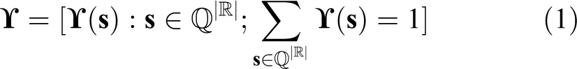To describe pulmonary nodules’ texture appearance, Gibbs energy values are calculated using the seventh-order MGRF model, to distinguish between benign and malignant nodules, because the Gibbs energy values show the interaction between the voxels and their neighbors¹⁹ (see Figure 4). The seventh order is used because it is the minimum order we could use, as we work on 3D volume, so at least we have to check the 6 neighbors of the voxel and the voxel itself. Using higher order than the seventh order will add more calculations with no noticeable enhancement in the framework accuracy. Let ℚ = {0,…, Q − 1} denote a finite set of signals (HU values) in the lung CT scan, s: ℝ³ → ℚ, with signals s = [s(r): r = (x, y, z) ∈ ℝ³]. The interaction graph, Γ = (ℝ³, 피), quantifies the signal probabilistic dependencies in the images with nodes at voxels, r ∈ ℝ³, that are connected with edges (r, r′) ∈ 피 ⊆ ℝ³ × ℝ³. An MGRF of images is defined by a Gibbs probability distribution (GPD):

Figure 3.

A 2-dimensional axial projection for 2 benign (A, B) and 2 malignant (C, D) lung nodules (first row), along their 3D visualization of Hounsfield values(second-row), and their calculated Gibbs energy (third-row).

Figure 4.

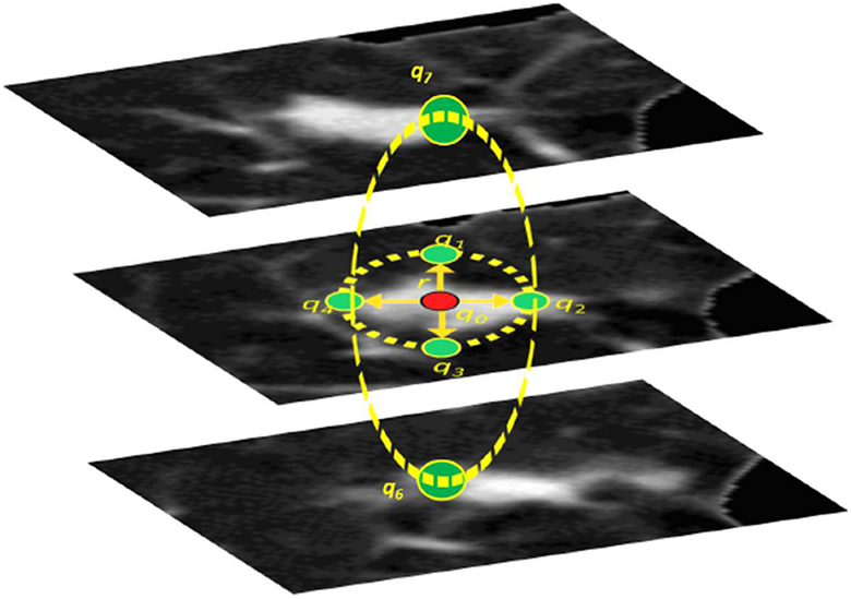
The seventh-order clique. Signals q ₀, q ₁,…, q ₆ are at the central pixel and its 6 central-symmetric neighbors at the radial distance r. Note that the selection of the neighborhood geometry takes into account the nodules sphericity.

ϒ = [ϒ (s) : s \in ℚ^{| ℝ |}; \sum_{s \in ℚ^{| ℝ |}} ϒ (s) = 1]

factored over a set ℂ of cliques in Γ supporting nonconstant factors, logarithms of which are Gibbs potentials.²⁰ To make modeling more efficient at describing the visual appearance of different nodules in the lung CT scans, the seventh-order MGRF models the voxel’s partial ordinal interaction within a radius r rather than modeling the pairwise interaction as in the second-order MGRF.

Let a translation-invariant seventh-order interaction structure on ℝ be represented by A, A ≥ 1, families, ℂa; a = 1,…, A, of seventh-order cliques, c _a _:r ∈ ℂa, of the same shape and size. Every clique is associated with a certain voxel (origin), r = (x, y, z) ∈ ℝ³, supporting the same (7)-variate scalar potential function, V_a : ℚ⁷ → (−∞, ∞).

The GPD for this contrast/offset-, and translation-invariant MGRF is

ϒ_{7} (s) = \frac{1}{Z} ϕ (s) exp (- Ε_{7} (s)),

where $E_{7 : a} (s) = \sum_{C_{a : r} \in ℂ_{a}} V_{7 : a} (g (r') : r' \in c_{a : r})$ and $E_{7} (s) = \sum_{a = 1}^{A} E_{7 : a} (s)$ denote the Gibbs energy for each individual and all the clique families, respectively; Z is a normalization factor, while ϕ(s) is a core distribution. The calculated Gibbs energy, E ₇(s), will be used to discriminate between benign and malignant tissues and gives an indication of malignancy. While a high potential of malignancy is indicated by lower energy, high potential to be benign is indicated by higher energy. To calculate E ₇(s), the Gibbs potentials for the seventh-order model are calculated using the maximum likelihood estimates (MLE) by generalizing the analytical approximation in^21,22:

V_{7 : a} (ξ) = \frac{F_{7 : a : core} (ξ) - F_{7 : a} (ξ | s °)}{F_{7 : a : core} (ξ) (1 - F_{7 : a : core} (ξ))},

where a = 1,…, A; ξ ∈ ϑ ₇, s ^○ denoted the training malignant nodule images; ξ denotes a numerical code of a particular seventh-order relation between the 7 signals on the clique; ϑ ₇ is a set of these codes for all seventh-order signal co-occurrences; F _7:a(s°) is an empirical marginal probability of the relation ξ; ξ ∈ ϑ ₇, over the seventh-order clique family C7:a for s °, and F _7:a:core(ξ) is the core probability distribution.

The proposed seventh-order MGRF appearance model is summarized in Algorithm 1.

Algorithm 1.

Learning the seventh-order MGRF appearance model.

1. Given a training malignant nodules g°, find the empirical nodule (l = 1) and background (l = 0) probability distributions, F _l _{:7: r}(g °) = [F_l _{:7: r}(β|g °): β ∈ 픹] of the local binary pattern-based descriptors for different clique sizes r ∈ {1,…, r _max} where the top size r _max = 10 in our experiments below.

2. Compute the empirical distributions F _7:r:core = [F _7:r:core(β): β ∈ 픹] of the same descriptors for the core independent random field ψ(g), for example, for an image, sampled from the core.

3. Compute the approximate MLE of the potentials:

V_{l : 7 : r} (β) = \frac{F_{7 : r : core} (β) - F_{l : 7 : r} (β | g °)}{F_{7 : r : core} (β) \cdot (1 - F_{7 : r : core} (β))} .

4. Compute partial Gibbs energies of the descriptors for equal and all other clique-wise signals over the training image for the clique sizes r = 1, 2,…, 10 to choose the size ρ_l , making both the energies the closest one to another.

Geometric Features

As the lung nodules have different geometric characteristics based on whether it is malignant or benign, accounting for these differences as a discriminating feature helps in the differentiation between different nodule types in the classification process. A set of 7 geometric features will be extracted from the nodule’s binary mask (provided by radiologist). The following geometric features are calculated: volume, surface area, convex volume, solidity, equivalent diameter, extent, and the principal axis length. In order to calculate the solidity, a convex hull C is defined around the segmented nodule and the ratio between the volume of the voxels in C and the total volume of the segmented nodule is calculated. Then, in order to calculate extent, the bounding box around the segmented nodule is used and the dimensions are named dimx, dimy, and dimz. To calculate extent, the proportion of the volume of the voxels in the bounding cube to the volume of the voxels of the segmented nodule is calculated. Principal axis length is defined as the largest dimension of the bounding cube (max(dimx, dimy, dimz)).

These features complement each other to come up with a final score for malignancy classification. To extract these features accurately without being dependent on scan accusation parameters such as pixel spacing and slice thickness, a volume of interest (VOI) of size 40 × 40 × 40 mm³ that is centered around the center of each nodule is extracted and resampled to be an isotropic in the x−, y−, and z− directions.

Nodule Classification Using Autoencoders

Our CADx system utilizes a feed-forward deep neural network to classify the pulmonary nodules whether malignant or benign, and the implemented deep neural network comprises 2-stage structure of stacked autoenocder (AE).

The first stage consists of 2 autoencoder-based classifiers, 1 classifier for the appearance and 1 for the geometry, which are used to give an initial estimation for the probabilities of the classification, that are augmented together to be considered as the input for the second-stage autoencoder to give the final estimation of the classification probabilities (see Figure 1 for more details).

Autoencoder is employed in order to diminish the dimensionality of the input data (1000 histogram bins for the Gibbs energy image in the network of the appearance) with multilayered neural networks to get the most discriminating features by greedy unsupervised pretraining.

After the AE layers, a softmax output layer is stacked in order to refine the classification by reducing the total loss for the training-labeled input. For each AE, let W = {W_j ^e, W_i ^d : j = 1,…, s; i = 1,…, n} refer to a set of column vectors of weights for encoding, E, and decoding, D, layers, and let T denote vector transposition. The AE change the n-dimensional column vector u = [u ₁,…, u_n ] ^T into an s-dimensional column vector h = [h ₁,…, h_s ] ^T of hidden features such that s < n by nonlinear uniform transformation of s weighted linear combinations of input as where σ(.) is a sigmoid function with values from [0,1], $σ (t) = \frac{1}{1 + e^{- t}}$ ,

Our classifier is constructed by stacking AE (see Figure 5) which consist of 3 hidden layers with softmax layer for the appearance network: the first hidden layer reduces the input vector to 500 level activators, while the second hidden layer continues the reduction to 300 level activators which are reduced to 100 after the third layer. The geometry network consists of the softmax layer only, as the input scale is not large enough to use AE with multiple hidden layers like the appearance network (only 9 geometric features) which compute the probability of being malignant or benign through the following equation:

Figure 5.

The proposed stacked autoencoder structure.

p (c; W_{o : c}) = \frac{e^{(W_{o : c}^{T} h^{3})}}{e^{(\sum_{1}^{c} W_{o : c}^{T} h^{3})}},

where C = 1 2; denote the class number W_o _:c: is the weighting vector for the softmax for class c; h ³: are the output features from the last hidden layer (the third layer) of the AE. In the second stage, the output probability obtained from the softmax of the appearance and geometry analysis networks are fused together and fed to another softmax layer to give the final classification probability.

Experimental Results

To train and test our proposed CADx system, the well-known LIDC data set is used. This data set consists of 1018 thoracic CT scans that have been collected from 1010 different patients from 7 different academic centers. After removing the scans with slice thickness greater than 3 mm and the scans with inconsistent slice spacing, a total of 888 CT scans became available for testing and evaluating our CADx system.²³ The LIDC CT scans are associated with an XML file to provide a well descriptive annotation and radiological diagnosis for the lung lesions, such as segmentation, shape, texture, and malignancy. All this information is provided by 4 thoracic radiologists in a 2-phase image annotation process. In the first phase, each radiologist from the 4 radiologists independently reviewed all cases and this phase is called blind read phase as each one gives their opinion regardless of the other radiologists. The second phase is the final phase as each radiologist gives his final decision after checking the other 3 radiologists’ decision, and this phase is called the unblinded phase as all the annotations were made available to all the radiologists before giving their final annotation decision. The radiologists divided the lesions into 2 groups, nodules and nonnodules. We focused on the nodules ≥3 mm as they have a malignancy score that vary from 1 as benign to 5 as malignant and a well-defined contour annotated by the radiologists.

We trained our CAD system on a randomly selected sample of nodules. In order to be sure that the data are almost balanced, we used 413 benign and 314 malignant nodules. For each nodule, the union of the 4 radiologists’ mask is combined to obtain the final nodule mask that we will use in ours (see Figure 6).

Figure 6.

Two-dimensional axial projection for 3 nodules and their masks. A, The mask as annotated by first radiologist. B, The mask as annotated by second radiologist. C, The mask as annotated by third radiologist. D, The mask as annotated by fourth radiologist. E, The combined mask for the 4 radiologists mask.

A VOI of size 40 × 40 × 40 mm measured around the center of the nodule’s combined mask is extracted for each nodule. The final diagnosis score of each nodule that we decided to work on is evaluated by calculating the average of the diagnosis scores for the 4 radiologists.

The system is evaluated using 10-fold cross-validation in order to be sure that every sample in the data set is eventually used for both training and testing. The classification accuracy is described in terms of different measurement metrics, namely, the specificity (true negative rate) that measures the percentage of negatives that are correctly identified (eg, the percentage of benign nodules that are correctly identified as benign), sensitivity (true positive rate) that measures the percentage of positives that are correctly identified (eg, the percentage of malignant nodules that are correctly identified as malignant), precision (positive predictive value) that measures the fraction of correctly identified as positives among the whole instances that identified as positives, accuracy that measures the fraction of correctly identified among the whole instances, and AUC. These measurements are calculated as follows:

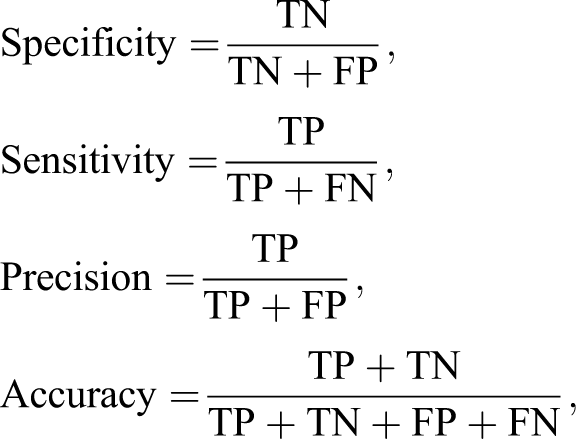
\begin{array}{l} Specificity= \frac{TN}{TN+FP}, \\ Sensitivity = \frac{TP}{TP + FN}, \\ Precision = \frac{TP}{TP + FP}, \\ Accuracy = \frac{TP + TN}{TP + TN + FP + FN}, \end{array}

where TP (true positive): correctly identified instances, FP (false positive): incorrectly identified instances, TN (true negative): correctly rejected instances, and FN (false negative): incorrectly rejected instances.

We reported the accuracy of the appearance model and the geometric model separately and for the complete fused system to highlight the effect of each model to the overall system (as shown in Table 1).

Table 1.

Classification of Results in Terms of Sensitivity, Specificity, Accuracy, Precession, and AUC for Different Feature Groups.

	Evaluation Metrics
	Sensitivity	Specificity	Accuracy	Precision	AUC
Geometric	82.80	88.14	85.83	84.14	92.02
Appearance	82.17	96.85	90.51	95.20	93.44
Comb. features	85.03	95.88	91.20	94.01	95.73

Abbreviations: AUC, area under the curve; comb., combined.

Boldface signifies the values with maximum accuracy.

Table 2 compares our system performance measures against other systems,^12,24,25 showing that our system has the lead in accuracy.

Table 2.

Comparison Between our Proposed System and Other 4 Recent Nodule Classification Techniques, in Terms of Sensitivity, Specificity, and Accuracy.

		Metric
		Sensitivity	Specificity	Accuracy
Method	Kumar et al ¹²	83.35	–	75.01
	Krewer et al ²⁴	85.71	94.74	90.91
	Jiang et al ²⁵	86.00	88.50	–
	Our system	85.03	95.88	91.20

Boldface signifies the values with maximum accuracy.

Figure 7 shows the ROC curve for each module and for the fused system as it is considered a powerful tool to evaluate the discrimination of binary outcomes (benign or malignant). The curve is created by plotting the sensitivity against 1 − the specificity at different threshold settings. The area under the ROC curve was 0.93, 0.92, and 0.96 for the appearance model, geometric model, and the fused system, respectively.

Figure 7.

Receiver operating characteristic curve for different feature classification and the combined ones.

Obviously the displayed features give a decent separation between benign and malignant nodules. In addition, the separation accuracy increased when these features combined using autoencoder. To validate the effectiveness of the autoencoder classifier, different classifiers are utilized for the combined features and compared with the framework accuracy that uses the autoencoder classifier. Random forest, SVM, and Naive Bayes classifiers are selected to be compared with the autoencoder and Table 3 shows the comparison between them.

Table 3.

Classification Results for the Deep Autoencoder Classifier Compared With RF, SVM, and NB Classifiers.

		Classifier Type
		AE	RF	SVM	NB
Metrics	Sens.	85.03	89.17	85.67	71.02
	Spec.	95.88	90.07	93.95	96.61
	Acc.	91.20	89.68	90.37	85.56

Abbreviations: Acc., accuracy; AE, autoencoder; NB, Naive Bayes; RF, random forest; SVM, support vector machine; Sens., sensitivity; Spec., specificity.

Boldface values signify the values which has maximum accuracy.

Discussion and Conclusion

The limitation of our framework is that although it is able to distinguish benign nodules from malignant ones, it could not differentiate between the different categories in each type. For example, the benign nodules have different categories like fibroma, hamartoma, neurofibroma, and blastoma, and the malignant nodules have different categories like lung cancer, lymphoma, carcinoid, sarcoma, and metastatic tumors. In particular, future work should seek an additional technique to distinguish also between the subclasses in each type of nodules.

In conclusion, this article introduced a novel framework for the classification of lung nodules by modeling the nodules’ appearance feature using a novel higher order MGRF in addition to geometric features. The classification results obtained from a set of 727 nodules collected from 467 patients confirm that the proposed framework holds the promise for the early detection of lung cancer. A quantitative comparison with recently developed diagnostic techniques highlights the advantages of the proposed framework over state-of-the-art ones. These promising results encourage us to model new shape features using spherical harmonic analysis and include it in the proposed framework to reach the clinically accepted accuracy threshold, which is ≥95.00%. Moreover, we plan to file an institutional review board protocol in the future and locally collect data at our site to test on subjects that have malignant/benign nodules with biopsy confirmations.

Footnotes

Declaration of Conflicting Interests

The author(s) declared no potential conflicts of interest with respect to the research, authorship, and/or publication of this article.

Funding

The author(s) received no financial support for the research, authorship, and/or publication of this article.

ORCID iD

Ayman El-Baz, PhD

Abbreviations

References

American Cancer Society. Cancer Facts and Figures. 2017.

Brazauskas

Ackman

Nelson

. Surveillance of actionable pulmonary nodules in children: the potential of thoracic MRI. Insight Chest Diseases. 2016;1:1–5.

Hua

, et al.

Can diffusion-weighted imaging be used as a reliable sequence in the detection of malignant pulmonary nodules and masses?

Magn Reson Imaging. 2013;31(2):235–246.

Thamilselvan

Sathiaseelan

JGR

. An enhanced k nearest neighbor method to detecting and classifying MRI lung cancer images for large amount data. Int J Appl Eng Res 2016;11(6):4223–4229.

Lee

Kouzani

. Random forest based lung nodule classification aided by clustering. Comput Med Imaging Graph. 2010;34(7):535–542.

Sun

Zheng

Qian

. Computer aided lung cancer diagnosis with deep learning algorithms. Paper presented at: Medical Imaging 2016: Computer-Aided Diagnosis. Volume 9785. International Society for Optics and Photonics. San Diego, CA; February 28, 2016, to March 2, 2016:97850Z. SPIE.

Likhitkar

Gawande

Hajari

. Automated detection of cancerous lung nodule from the computed tomography images. IOSR J Comput Eng. 2014;16(1):5–11.

Wei

Qian

, et al. Lung nodule classification using local kernel regression models with out-of-sample extension. Biomed Signal Process Control. 2018;40:1–9.

Nishio

Nagashima

. Computer-aided diagnosis for lung cancer: usefulness of nodule heterogeneity. Acad Radiol. 2017;24(3):328–336.

10.

Dhara

Mukhopadhyay

Dutta

Garg

Khandelwal

. A combination of shape and texture features for classification of pulmonary nodules in lung CT images. J Digit Imaging. 2016;29(4):466–475.

11.

Firmino

Angelo

Morais

Dantas

Valentim

. Computer-aided detection (CADe) and diagnosis (CADx) system for lung cancer with likelihood of malignancy. Biomed Eng Online. 2016;15(1):2.

12.

Kumar

, et al. Lung nodule classification using deep features in CT images. Paper presented at: Computer and Robot Vision (CRV), 2015 12th Conference. Halifax, Nova Scotia, Canada; June 3–5, 2015. 133–138. IEEE.

13.

Song

Zhao

Luo

Dou

. Using deep learning for classification of lung nodules on computed tomography images. J Healthc Eng. 2017;2017:8314740.

14.

Xie

Zhang

Xia

Micheal

Zhang

. Fusing texture, shape and deep model-learned information at decision level for automated classification of lung nodules on chest ct. Informat Fusion. 2018;42:102–110.

15.

Guo

Yen

El Fakhri

, et al. SVM based lung cancer diagnosis using multiple image features in PET/CT. In: Nuclear Science Symposium and Medical Imaging Conference (NSS/MIC), 2015, pp. 1–4, IEEE.

16.

ur Rehman

Javaid

Shah

SIA

, et al. An appraisal of nodules detection techniques for lung cancer in CT images. Biomed Signal Process Control. 2018;41:140–151.

17.

Liu

Hou

Qin

Hao

. Multi-view multi-scale CNNs for lung nodule type classification from CT images. Pattern Recognition. 2018;77(C):262–275.

18.

Shaffie

Soliman

Ghazal

, et al. A new framework for incorporating appearance and shape features of lung nodules for precise diagnosis of lung cancer. Paper presented at: Image processing (ICIP), 2017 IEEE International Conference. Beijing, China, 17–20 September 2017, 1372–1376. IEEE.

19.

Liu

Soliman

Gimelfarb

El-Baz

. Segmenting kidney DCE-MRI using 1st-order shape and 5th-Order appearance priors. Paper presented at: International Conference on Medical Image Computing and Computer-Assisted Intervention, 2015, pp. 77–84. Munich, Germany: Springer.

20.

Blake

Kohli

Rother

. Markov Random Fields for Vision and Image Processing. Cambridge, USA: MIT Press; 2011.

21.

GimelFarb

Farag

. Texture analysis by accurate identification of simple markovian models. Cybern Syst Anal. 2005;41(1):27–38.

22.

El-Baz

Gimelfarb

Suri

. Stochastic Modeling for Medical Image Analysis. Boca Raton, USA: CRC Press; 2015.

23.

Armato

SG III

McLennan

Bidaut

, et al. The Lung Image Database Consortium (LIDC) and Image Database Resource Initiative (IDRI): a completed reference database of lung nodules on CT scans. Med Phys. 2011;38(2):915–931.

24.

Krewer

Geiger

Hall

, et al. Effect of texture features in computer aided diagnosis of pulmonary nodules in low-dose computed tomography. Paper presented at: Systems, Man, and Cybernetics (SMC), 2013 IEEE International Conference; Manchester, United Kingdom; October 13-16, 2013:3887–3891. IEEE.

25.

Jiang

Qian

Wei

Zhoa

Gao

. A novel pixel value space statistics map of the pulmonary nodule for classification in computerized tomography images. Paper presented at: Engineering in Medicine and Biology Society (EMBC), 2017 39th Annual International Conference of the IEEE; Seogwipo, South Korea; July 11-15, 2017:556–559. IEEE.

A Generalized Deep Learning-Based Diagnostic System for Early Diagnosis of Various Types of Pulmonary Nodules

Abstract

Keywords

Introduction

Methods

Appearance Features Using MGRF Energy

Geometric Features

Nodule Classification Using Autoencoders

Experimental Results

Discussion and Conclusion

Footnotes

Declaration of Conflicting Interests

Funding

ORCID iD

Abbreviations

References