Sage Journals: Discover world-class research

Abstract

We use random forests, a machine-learning technique, to formally examine the link between real gasoline prices and presidential approval ratings of the United States (US). Random forests make it possible to study this link in a completely data-driven way, such that nonlinearities in the data can easily be detected and a large number of control variables, in line with the extant literature, can be considered. Our empirical findings show that the link between real gasoline prices and the presidential approval ratings is indeed nonlinear, and that the former even has predictive value in an out-of-sample exercise for the latter. We argue that our findings are in line with the so-called pocketbook mechanism, which stipulates that the presidential approval ratings depend on gasoline prices because the latter have sizable impact on personal economic situations of voters.

Keywords

presidential approval ratings gasoline price random forests forecasting C22 C53 Q40 Q43

Introduction

There is quite a lot of discussion in the popular media about the possible negative influence of gasoline prices on the presidential approval ratings of the United States (US).¹ Although various government policies (like import tariffs, infrastructure investment, renewable energy-related decisions, and environmental standards) can move gasoline prices in one direction or another, the fact is that US presidents actually have only limited control over energy prices, which are determined by global supply and demand. Hence, the frequent politicization of gasoline prices might seem puzzling. However, as outlined in Kim and Yang (2022), two mechanisms can account for the electoral effects of gasoline prices. First, voters response to changes in gasoline price may reflect “pocketbook” considerations, i.e., changes in gasoline prices can result in sizable gains or losses for individual voters, and hence, may affect their personal economic situations. Second, voters can be motivated by a “sociotropic” reason, that is, voters may consider movements in gasoline prices as an informational source about the general health of the economy.

In this research, our objective aim is to test this relationship between the US presidential approval ratings and gasoline prices by accounting for nonlinearity, as confirmed by statistical tests conducted by us, as well as, by controlling for a large number of macroeconomic and financial factors, and their corresponding uncertainties, besides geopolitical risks, and oil prices. The importance of these variables has been highlighted in many studies (see, for instance, Burden and Mughan (2003); Halcoussis et al. (2009); Chong et al. (2011); Fauvelle-Aymar and Stegmaier (2013); Berlemann and Enkelmann (2014); Berlemann et al. (2015); Choi et al. (2016); Dickerson (2016); Adrangi and Macri (2019); Gupta et al. (2021); Bouri et al. (2024), and references cited therein). Specifically, several researchers have emphasized that these variables often act as nonlinear drivers for the US presidential approval ratings in the sense that their impact becomes strong and/or significant in a statistical sense once they increase beyond a certain threshold. Choi et al. (2016), for example, explicitly formulate and test the hypothesis that the effects of economic conditions on presidential approval ratings take on a nonlinear form, where they motivate this hypothesis by pointing out that threshold effects may be a characteristic feature of media coverage of the economy in general and of specific economic variables in particular. Hence, in case of our research, it is plausible to stipulate that the impact of real gasoline prices on the US presidential approval ratings is negative but small due to moderate media coverage when gasoline prices start increasing from a low level. When real gasoline prices start increasing further, however, things are likely to change as media coverage most likely increases sharply, and a higher share of perhaps formerly inattentive voters realizes that the purchasing power of money is decreasing, thereby lowering the presidential approval ratings and giving rise to the kind of threshold effects documented in the empirical literature involving the macroeconomic predictors. At the same time, when real gasoline prices increase even further, the presidential approval ratings, having already dropped to a lower level, and in the wake of continuing media coverage, dissatisfied voters most likely to some extent get used to higher real gasoline prices, implying that, once the threshold level of real gasoline prices has been crossed, the presidential approval ratings stays at a comparatively low level or further decreases moderately. In terms of empirical research, Berlemann and Enkelmann (2014) argue that nonlinear links between the US presidential approval ratings and economic indicators may account for inconclusive and sometimes conflicting results documented in the extant earlier studies, and Berlemann and Enkelmann (2014) present evidence of nonlinearities.

Given the potential importance of nonlinear links between economic indicators and US presidential approval ratings, it is important to account for such nonlinearities in empirical research, i.e., in terms of the empirical model being used, without restricting a priori the shape of a potential nonlinearity, that is, it is desirable to capture any nonlinear structure in the data in a fully data-driven way. Econometrically speaking, we address the question in hand in a robust manner by means of a machine learning approach, known as random forests (Breiman, 2001), over the monthly period of 1973:10 to 2023:12. Random forests can accurately trace out the link between presidential approval ratings and a large number of its drivers, which in our case is 19 (including the lagged presidential approval ratings), in a full-fledged data-driven manner. Being a nonparametric approach, random forests automatically capture potential nonlinear links between the US presidential approval ratings and gasoline prices, besides the various other control variables.

To the best of our knowledge, we are the first to analyze whether there is a prominent role of gasoline prices in driving US presidential approval ratings using a machine-learning approach. More importantly, we not only consider this question from an in-sample view, but also conduct a one-step-ahead out-of-sample forecasting exercise, with the latter well-established as a relatively stronger test of predictability than an in-sample test (Campbell, 2008). In the process, our research can be considered to be an extension to the somewhat related studies of Harbridge et al. (2016) and Coggin (2024). In Harbridge et al. (2016), the authors assessed the strength of the pocketbook and the sociotropic mechanisms by examining the interaction effects between gasoline prices and media coverage volume on presidential approval ratings, the idea being that, if the sociotropic mechanism prevails, the impact of gasoline prices should be more significant when voters are exposed to more regular news coverage about gasoline prices. Relying on data from multiple surveys, Harbridge et al. (2016) reported an insignificant effect from the interaction term along with independent effects from gasoline prices, thus, suggesting a strong pocketbook but weak sociotropic mechanism.² As far as the recent work of Coggin (2024) is concerned, this paper highlighted the importance of gasoline prices in producing a reduction in US presidential approval ratings in a linear set-up with a handful (eight) other predictors as control variables, and, in the process, emphasized the pocketbook channel. In this regard, our paper can be considered as an improvement to the work of Coggin (2024), especially methodologically, as we address the issue of potential misspecification of the linear model, given the evidence of nonlinear association between the variables of interest in our nonparametric set-up. Moreover, the number of variables considered by Coggin (2024) was also limited compared to that of ours, and, hence, we prevent the possibility of the so-called “omitted-variables-bias”. Finally, the study by Coggin (2024) was only restricted to in-sample deductions, with no evidence of the associated possible forecasting power of gasoline prices for US presidential approval ratings, as done by us, which, in turn, is a well-known relatively stronger statistical test of the validity of predictability.

Given that the US elections just concluded with a new president-elect at the end of 2024, and the fluctuations in gasoline (and oil) prices constantly in the news, especially in the wake of a series of recent geopolitical events associated with major energy-producing economies, this is indeed a pertinent question to ask. Answering this question is not only of paramount importance from the perspective of global investors operating in financial markets (on political cycles and stock-market returns, see Pástor and Veronesi, 2020), but also from the point of view of world politics, due to the worldwide influence of (divergent) policy stances undertaken by Democratic and Republican presidents. At the same time, while our objective is not necessarily to explicitly identify the channels through which gasoline prices drive the US presidential approval ratings, if we end up finding that the former are indeed relatively more important (as is possible in our machine-learning set-up) than the macroeconomic factors, as well as oil prices (historically known to be closely associated with the US macroeconomy and financial markets, Gupta & Wohar, 2017), in impacting the latter, such a finding can be interpreted as a further piece of evidence in line with the pocketbook mechanism. This is because, if voters use real gasoline prices as carrying information about the state of the economy, then the link between real gasoline prices and the presidential approval ratings should weaken, or even no longer exist in the extreme scenario, once we include macroeconomic and financial predictors in our model that tends to capture the uncertainty and expectations of voters about future macroeconomic developments, in light of the close relationship between gasoline prices and macroeconomic outcomes (see Baumeister et al. (2017) for a detailed discussion). In light of this, at the same time, the empirical results of our paper could also be relevant academically to the theoretical literature on electoral politics, which aims to identify underlying reasons (i.e., pocketbook or sociotropic) behind economic voting (Fiorina, 1981; Gomez & Wilson, 2001; Kinder & Kiewiet, 1981; Kramer, 1971).

Previewing our results, we report that the link between real gasoline prices and the US presidential approval ratings is nonlinear in nature, with the former being a relatively more important predictor than the wide array of other macroeconomic and financial controls, to the extent that it also carries an out-of-sample forecasting value for the approval ratings. At this juncture, it must be emphasized that our findings are likely to carry limited policy implications, beyond reducing taxes and import tariffs, given that US presidents cannot necessarily control gasoline, which, in turn, are governed by worldwide supply and demand. We organize the remainder of this research as follows: In Section 2, we provide a description of the data that we use in our study, while we outline in Section 3 our econometric model. In Section 4, we present our empirical results. In Section 5, we conclude.

Data

The data on US presidential approval ratings (PAR) are based on surveys conducted by Gallup, as part of the American Presidency Project.³ A rating (expressed in percentage terms) informs about the proportion of respondents to an opinion poll who approve of the US president in office at the time when the poll was conducted. An important advantage of the Gallup poll, which differentiates it from other national polls informing about public approval of the president, is that the Gallup poll has been based over the years (since, July, 1941) on the same unchanged approval question: “Do you approve or disapprove of the way [enter president name] is handling his job as president?”. The upper panel of Figure 1 plots the ups and downs of the presidential approval ratings during the sample period that we study in this research.

Figure 1.

Presidential approval ratings and real gasoline prices.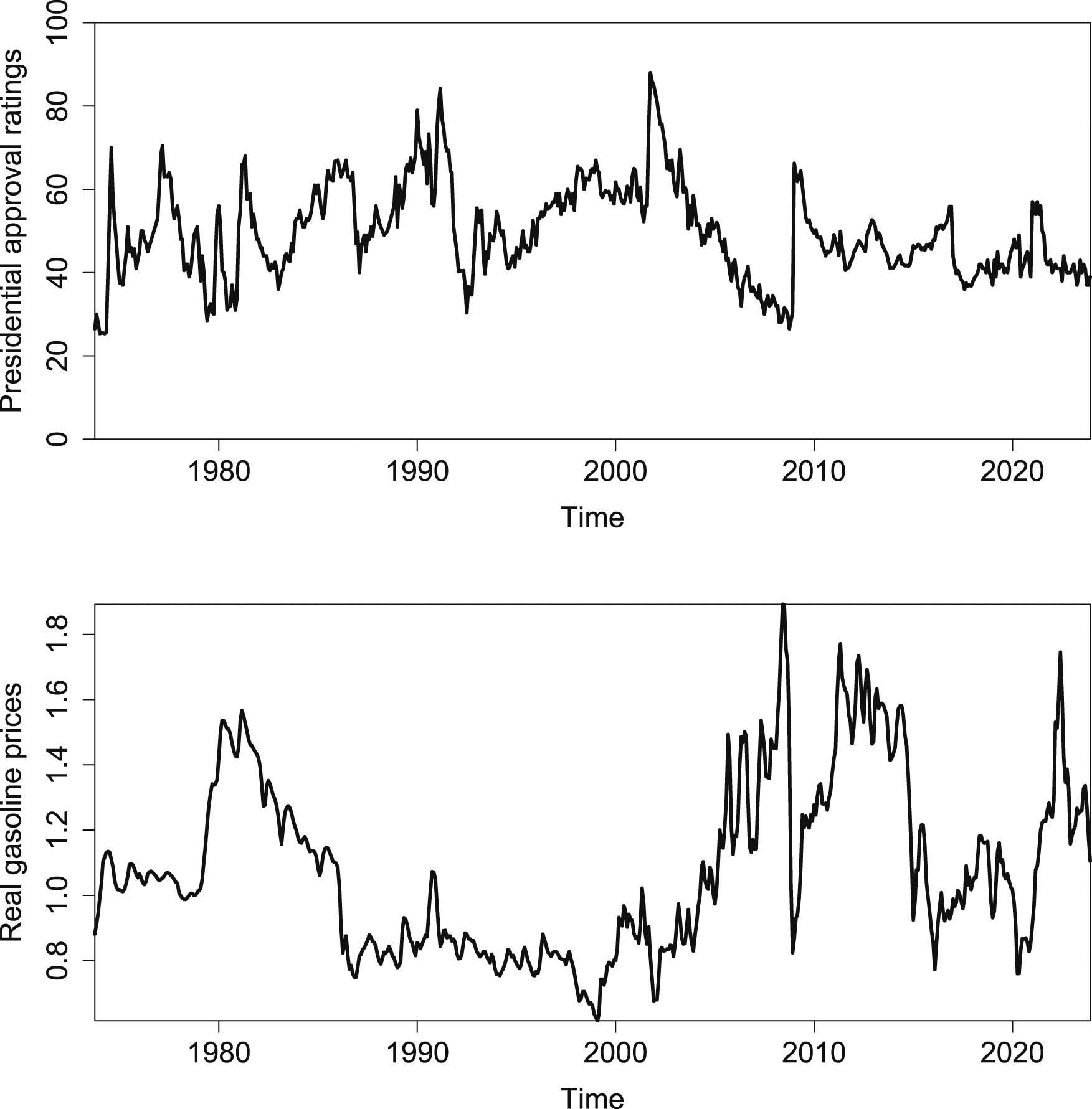

As far as nominal gasoline prices are concerned, we utilize the US city average of all grades of gasoline retail price (in dollars per gallon including taxes). The data is obtained from the Monthly Energy Review of the Energy Information Administration (EIA) of the US.⁴ We obtain real gasoline prices (RGP) by deflating with the Consumer Price Index (CPI), which captures the average price of all items for all urban consumers, obtained from the FRED database maintained by the Federal Reserve Bank of St. Louis.⁵ The lower panel of Figure 1 plots real gasoline prices.

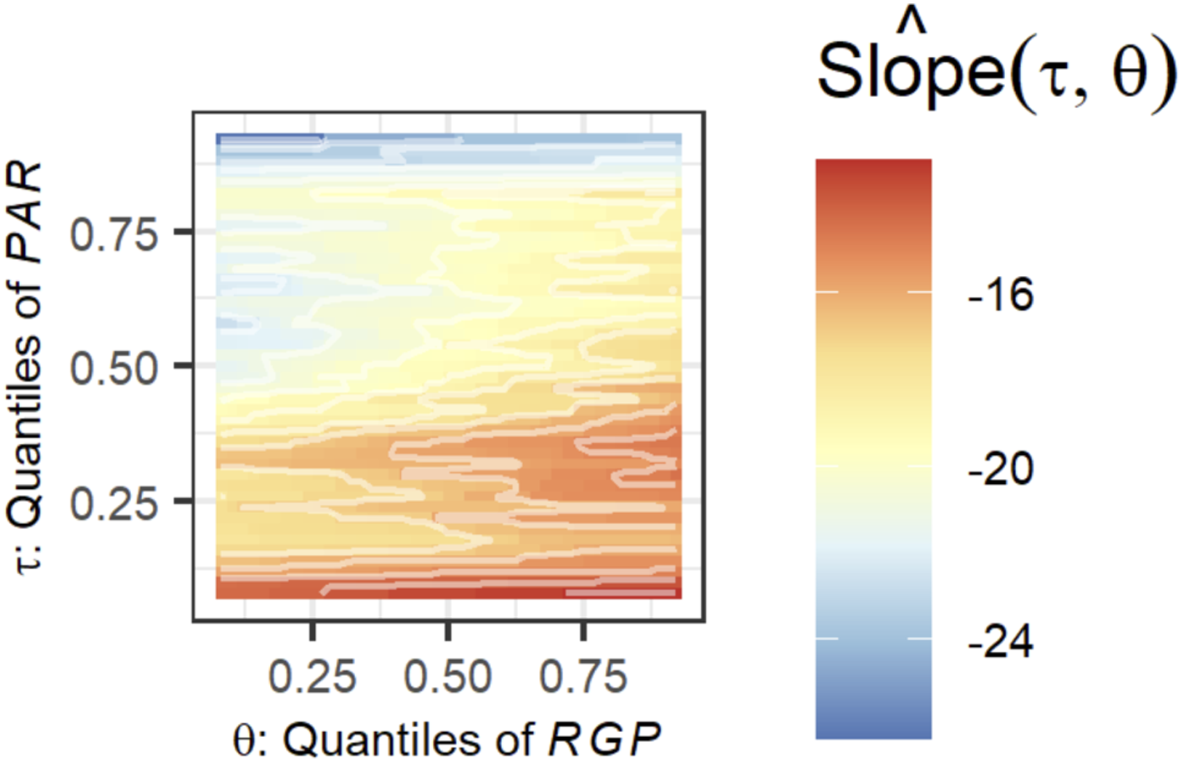
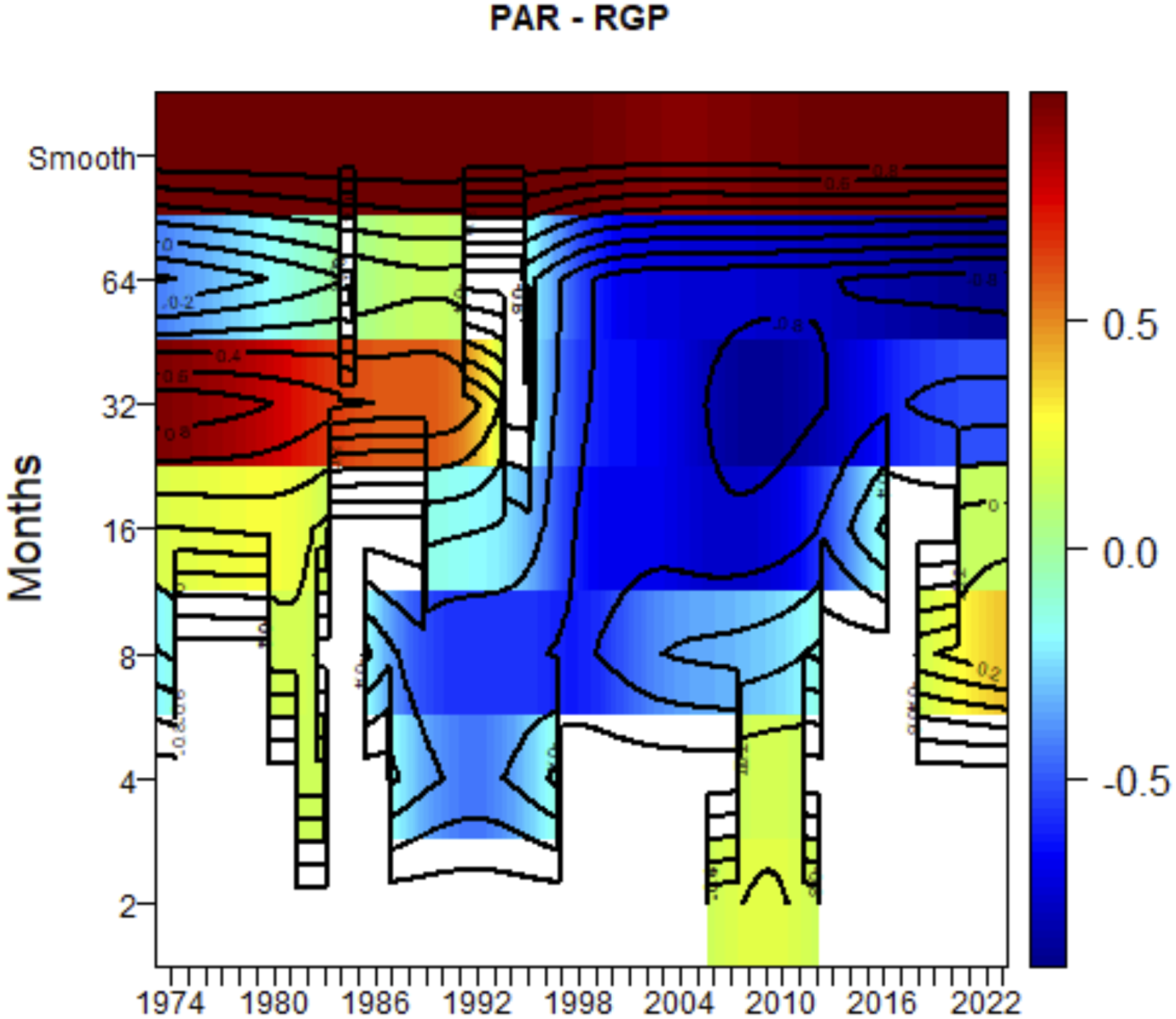
Browsing through Figure 1, there does seem to be a negative association between PAR and RGP, as is confirmed by a negative full-sample correlation coefficient of = −0.46, with a p-value of 0.00. The empirical fact that this negative association is nonlinear, however, is indicated when we estimate a quantile-on-quantile regression model, in line with Sim and Zhou (2015). We find, as reported in Figure A1 at the end of the paper (Appendix), that the effect varies in magnitude across the conditional quantiles of PAR for different sized-values (quantiles) of RGP, with relatively stronger effects at lower quantiles of the latter and upper quantiles of the former. Using the wavelet localized multiple correlation (WLMC) approach of Fernández-Macho (2018), the nonlinear negative relationship of RGP with PAR is, in general, confirmed not only based on varying strength of correlation over time, but also across frequency-bands, particularly over to medium- to long-run since the mid-1980s, as shown in Figure A2, which we also place at the end of the paper.

We also control for crude oil prices by utilizing the real values of the Cushing, Oklahama West Texas Intermediate (WTI) spot oil price (RWTI), with the nominal price also derived from the EIA,⁶ and the CPI deflator from the FRED. As has been emphasized by Kilian (2010), while crude oil is the main input in the production of motor gasoline, the retail prices of the latter will in addition reflect shocks to the demand from the US for gasoline as well as shocks to the ability of US-based refiners to process crude oil. In other words, changes in the retail price of gasoline are likely to be driven not exclusively by events in the global crude oil market. It, thus, is important to look at both gasoline and oil separately when considering the role of energy prices in impacting the presidential approval ratings.

We now turn our attention to a detailed discussion of our other predictors, beyond the energy prices. In order to capture a broad base of macroeconomic and financial variables, in line with the literature on presidential approval ratings mentioned above, we use eight factors (F1, F2,…, F8) derived from the 134 macroeconomic variables of Ludvigson and Ng (2009, 2011).⁷ Including these factors gives us the advantage of capturing a wide array of aggregate and regional time-series. The factors contain information on real output and income, employment and hours, real retail, manufacturing and sales data, international trade, consumer spending, housing starts, housing building permits, inventories and inventory sales ratios, orders and unfilled orders, compensation and labor costs, capacity utilization measures, price indexes, interest rates and interest rate spreads, stock market indicators, and foreign exchange measures. As pointed out by Ludvigson and Ng (2009, 2011), the factors can be distinctly identified with F1 being a real activity factor, F2 capturing interest rate spreads, F3 and F4 capturing comovements of prices, F5 being an interest rates factor, F6 and F8 capturing the situation in the housing and the stock markets, and, finally, F7 summarizing the alternative measures of the money supply.

In addition, in line with earlier studies dealing with what determines US presidential approval ratings, we use the macroeconomic uncertainty (MU) and financial uncertainty (FU) measures developed by Jurado et al. (2015) and Ludvigson et al. (2021), which, in turn, is the average time-varying variance in the unpredictable component of 134 macroeconomic and 148 financial time-series. In other words, the MU and FU variables are designed in a way so as to capture the average volatility in the shocks to the factors that summarize real and financial conditions.⁸ The metrics that we use are the broadest measures of macroeconomic and financial uncertainties currently available for the US. The uncertainty indexes cover three forecasting horizons of 1-, 3-,and 12-month-ahead, and are denoted by MU1, MU3, MU12, FU1, FU3, and FU12.

Again, in line with earlier research on the topic of presidential approval ratings, as far as geopolitical risks are concerned, we consider two indexes related to threats and attacks. The two indexes are based on the work by Caldara and Iacoviello (2022),⁹ who compute the indexes by counting the number of articles related to adverse geopolitical events using automated text search of the electronic archives of three newspapers (namely, the Chicago Tribune, the New York Times, and the Washington Post) for each month (as a share of the total number of news articles). The search spans eight categories (war threats, peace threats, military buildups, nuclear threats, terror threats, beginning of war, escalation of war, terror acts), with the geopolitical threats (GPRT) index covering categories 1 to 5, and the geopolitical acts (GPRA) index comprising of categories 6 to 8.

Understandably, along with a lag of presidential approval ratings, included to capture the persistence of the presidential approval ratings, we end up with 19 predictors of the presidential approval ratings for the current period, covering the monthly sample period ranging from 1973:10 to 2023:12, based on data availability at the time of writing this paper, with the start date corresponding to the RGP series,¹⁰ and the end date being in line with the eight factors and the six uncertainty measures.

Random Forests

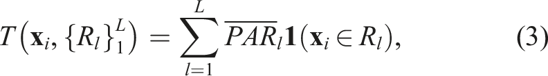
In order to detect the nature of the link between the presidential approval rating, PAR and real gasoline prices, RGP, we use models of the following format:

P A R_{t} = f (P A R_{t - 1}, R G P_{t}, C V_{t}),

(1)

where CV_t denotes a vector of the 17 control variables (i.e., eigth macro and financial factors (F1, F2,…, F8); six uncertainty-related measures (MU1, MU3, MU12, FU1, FU3, FU12); two geopolitical risks indexes (GPRT, GPRA), and RWTI), and f(.) is a function to be estimated. We estimate this function using random forests (Breiman, 2001). A random forest consists of a large number of individual regression trees, T, which are combined in an additive way. A regression tree, in turn, consists of a root and several nodes and branches (see, Breiman et al. (1984)). The nodes and branches partition the space of the predictors into non-overlapping regions, which are identified by applying a search-and-split algorithm (for a textbook exposition, see Hastie et al. (2009)). This search-and-split algorithm is initialized at the root of a regression tree by subdividing the space of predictors into a left region (i.e., a branch), R₁, and a right region, R₂, which are identified by searching for combination of a predictor and a splitting point, {s, p}, that solves the following optimization problem:

\min_{s, p} \{\min_{{\bar{P A R}}_{1}} \sum_{x_{s} \in R_{1} (s, p)} {(P A R_{z} - {\bar{P A R}}_{1})}^{2} + \min_{{\bar{P A R}}_{2}} \sum_{x_{s} \in R_{2} (s, p)} {(P A R_{z} - {\bar{P A R}}_{2})}^{2}\} \to {s^{*}, p^{*}},

(2)

where x_s denotes a realization of predictor s, an asterisk denotes an optimal value, z identifies those realizations of PAR that belong to a region, and

{\bar{P A R}}_{k}, k = 1,2

denote the region-specific means of PAR.

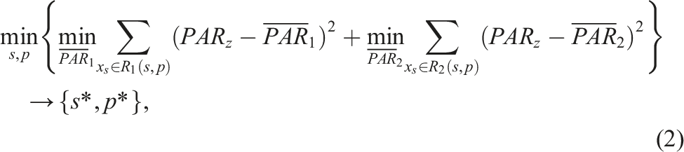
Upon applying the search-and-split algorithm in top-down way by applying this optimization problem in a recursive way, we can grow a complex regression tree that consists of many nodes and branches. The predicted value of the presidential approval ratings then can be computed from such a regression tree as follows:

T (x_{i}, {R_{l}}_{1}^{L}) = \sum_{l = 1}^{L} {\bar{P A R}}_{l} 1 (x_{i} \in R_{l}),

(3)

where L denotes the number of regions and 1 denotes the indicator function.

A complex regression tree should inform a researcher in much detail about the link between the presidential approval ratings, the real gasoline price, and the vector of control variables. At the same time, its complicated hierarchical structure makes a complex regression tree rather sensitive to the specific idiosyncratic features of the sample of data under study. A random forest addresses this overfitting problem by growing not only one but many regression trees. Such an ensemble of regression trees is grown by (i) computing a large number of bootstrap samples by resampling from the data, (ii) growing a random regression tree for every single bootstrap sample, and (iii) predict the presidential approval ratings as the average prediction obtained from the ensemble of random regression trees. A random regression tree uses for the search-and-splitting algorithm only a random subset of the predictors and, thereby, mitigates the effect of influential predictors on tree building. Averaging across random regression trees, in turn, stabilizes the resulting predictions.

We use the R language and environment for statistical computing (R Core Team, 2023) and the R add-on package “randomForestSRC” (Ishwaran & Kogalur, 2023) to estimate random forests. We use 500 individual regression trees to grow a random forest, and bootstrapping is done with replacement.

Empirical Results

We start our empirical analysis with a brief look at the results of a conventional ordinary-least-squares (OLS) model. This OLS model features only the lagged presidential approval ratings and real gasoline prices as predictors, but not the other control variables. The OLS model, thus, sheds light on the bivariate linear correlation between the presidential approval ratings and real gasoline prices, after accounting for the persistence of the former. Table 1 summarizes the results of estimating the OLS model. The coefficient of the lagged presidential approval ratings is estimated to be approximately 0.91, while the coefficient estimated for real gasoline prices takes on a value of roughly −1.99. Both coefficients are individually highly significant statistically, and also their total explanatory power, as summarized by the F-statistic, is highly significant. The adjusted R² of the OLS model is approximately 0.87, indicating that the fit of the model is satisfactory. The main message to take home from the OLS model is that the contemporaneous correlation between the presidential approval ratings and real gasoline prices is significantly negative.

Table 1.

OLS Results.

Predictor	Coefficient	t-value
Intercept	6.7445	3.8340^a
PAR lag	0.9077	40.4991^a
Real gasoline prices	−1.9970	−2.6794^a
Adjusted R²	0.8679
F_2,600DF (p-value)	<0.0001

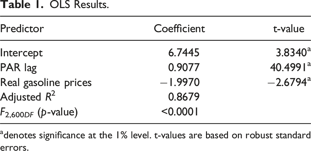
^adenotes significance at the 1% level. t-values are based on robust standard errors.

The OLS model imposes a linear structure on the data. The results that we summarize in Figure 2 indicate that such a linear structure may be too restrictive.¹¹ Figure 2 shows a scatterplot of the presidential approval ratings as a function of real gasoline prices along with a superimposed local Gaussian polynomial regression and its ± 2 standard error band. In line with the OLS results, the polynomial regression function has a negative slope as well. The local slope of the polynomial regression function, however, in addition reveals that, at comparatively low values of real gasoline prices, the correlation is stronger (in absolute terms) than at relatively high values of the real gasoline price. Hence, the estimated polynomial regression function indicates that the contemporaneous link between the presidential approval ratings and real gasoline prices is nonlinear.

Figure 2.

Local Gaussian polynomial regression. Dashed gray lines denote the boundaries of a ± two standard error band.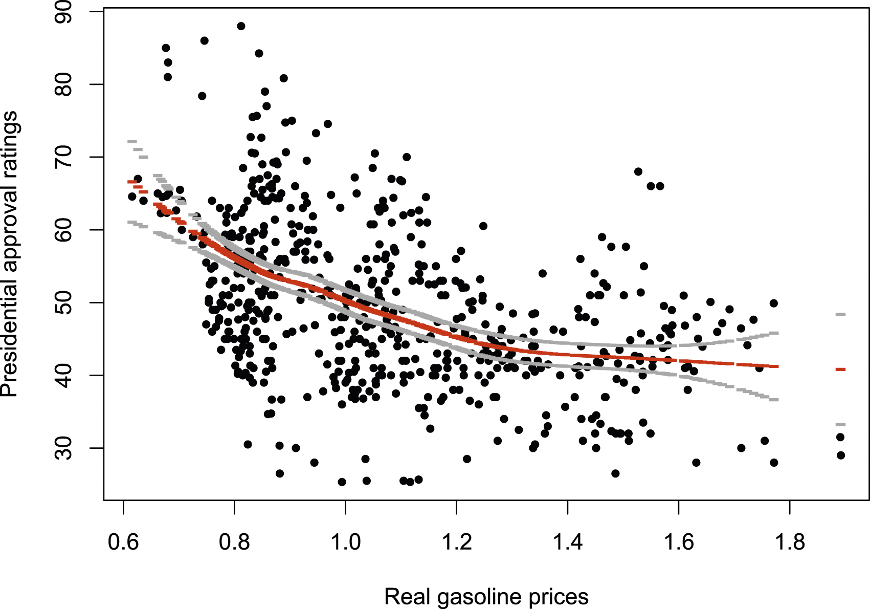

Like the OLS model that we consider in Table 1, the polynomial regression does not control for the impact of the predictors other than real gasoline prices. While it would be possible to include several other predictors in the OLS model in addition to real gasoline prices so as to trace out the incremental impact of real gasoline prices on the presidential approval ratings, such a research strategy runs into several difficulties. First, such an empirical modeling strategy would yield a high-dimensional but highly unreliable model in case nonlinearities in fact are present in the data. Second, such an empirical modeling strategy would result in an OLS model that, while already being complex, still would be incomplete because it only would be natural to account for a nonlinearity not only with regard to real gasoline prices, but rather with regard to the other predictors as well. Third, it would be important to account for potential interaction effects between the predictors because, for example, the impact of real gasoline prices on the presidential approval ratings may depend in a potentially complex way on the level of macroeconomic uncertainty. Such interaction effects further would inflate the number of predictors included in an OLS model. Finally, even after adding a full set of nonlinear and interactions terms to an OLS model, a researcher would still have to decide on the specific form of nonlinearities and interaction effects, further proliferating the space of models from which to choose arbitrarily a specific model for estimation and forecasting. Given these difficulties, it should be clear that random forests are a much better model to inspect how the presidential approval ratings are linked to real gasoline prices.¹²

In order to shed light on the link between the presidential approval ratings and real gasoline prices after controlling for the predictive value of the other predictors, we plot in Figure 3 the partial dependence function we obtain from estimating a random forest. The partial dependence function informs about the value of the presidential approval ratings that the estimated random forest predicts for alternative realizations of real gasoline prices, holding the other predictors constant. The estimated partial dependence function resembles the estimated polynomial regression function. The partial dependence function has a strongly negative slope for low values of real gasoline prices and then more or less flattens out when real gasoline prices increase beyond their mean (1.08)/median (1.03).

Figure 3.

Partial dependence plot. Dashed red lines denote the smoothed boundaries of a± two standard error band.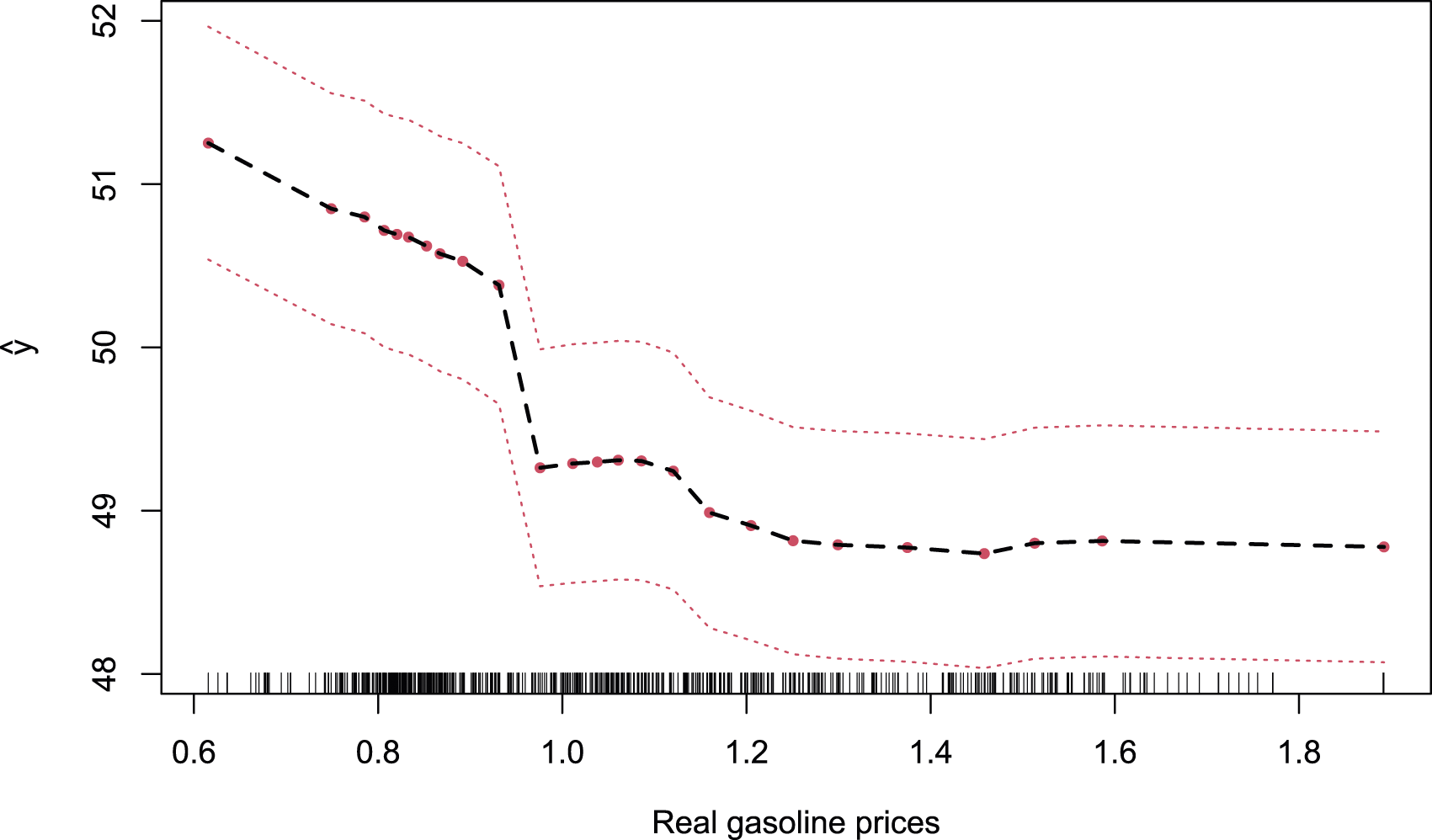

Another way to look at the link between the presidential approval ratings and real gasoline prices is to use the estimated random forest to study the variable importance (VIMP) of the latter. Alternative definitions of VIMP can be used to this end. Table 2 depicts the results for two such definitions. For the upper panel, permuted out-of-bag data are trickled down a tree and for every tree the difference is computed between the prediction error obtained using the predictor noised-up in this way and the original predictor. VIMP is then computed as the average of this difference across all trees in the estimated random forest. For the lower panel, VIMP is computed as an overall forest effect by comparing all perturbed and unperturbed trees in the estimated random forest. In other words, the left panel shows VIMP as an average tree effect, while the right panel shows VIMP as an overall forest effect. Both panels, however, convey the same message. The lagged presidential approval rating is the most important predictor, followed by real gasoline prices and the real oil price (or the other way round).

Table 2.

Variable Importance.

CI	PAR _t−1	F1	F2	F3	F4	F5	F6	F7	F8	MU1	MU3	MU12	FU1	FU3	FU12	GPRHT	GPRHA	RWTI	RGP
Panel A: Tree average effect
2.5	103.94	0.57	−0.45	−0.21	0.29	0.08	1.32	−0.14	−0.18	1.34	1.49	1.93	1.02	1.06	1.36	0.68	0.47	5.08	6.73
25	114.62	1.03	−0.09	0.15	0.65	0.39	2.05	0.03	0.12	2.02	2.47	4.17	2.23	1.71	2.49	1.07	1.85	6.76	8.45
50	120.23	1.28	0.09	0.34	0.84	0.55	2.43	0.13	0.27	2.38	2.98	5.34	2.86	2.05	3.08	1.28	2.57	7.64	9.36
75	125.83	1.52	0.27	0.53	1.03	0.71	2.82	0.22	0.43	2.74	3.45	6.52	3.45	2.40	3.68	1.48	3.23	8.53	10.26
97.5	136.51	1.99	0.63	0.89	1.34	1.02	3.55	0.39	0.73	3.43	4.48	8.76	4.71	3.05	4.81	1.87	4.68	10.21	11.98
Panel B: Overall forest effect
CI	PAR _t−1	F1	F2	F3	F4	F5	F6	F7	F8	MU1	MU3	MU12	FU1	FU3	FU12	GPRHT	GPRHA	RWTI	RGP
2.5	55.52	0.02	−0.47	−0.23	−0.26	−0.25	−0.05	−0.17	−0.14	−0.21	−0.15	0.02	0.04	0.04	0.07	−0.16	0.19	0.70	0.26
25	60.26	0.19	−0.25	−0.06	−0.11	−0.10	0.23	−0.08	−0.02	−0.07	0.04	0.26	0.32	0.22	0.24	−0.03	0.71	1.19	0.87
50	62.75	0.29	−0.14	0.04	−0.03	−0.01	0.38	−0.03	0.05	0.01	0.14	0.38	0.46	0.31	0.33	0.04	0.98	1.44	1.19
75	65.23	0.38	−0.02	0.13	0.05	0.07	0.53	0.02	0.11	0.08	0.24	0.51	0.61	0.41	0.43	0.11	1.25	1.69	1.51
97.5	69.98	0.56	0.20	0.30	0.19	0.23	0.81	0.11	0.23	0.23	0.42	0.75	0.88	0.59	0.60	0.24	1.77	2.17	2.12

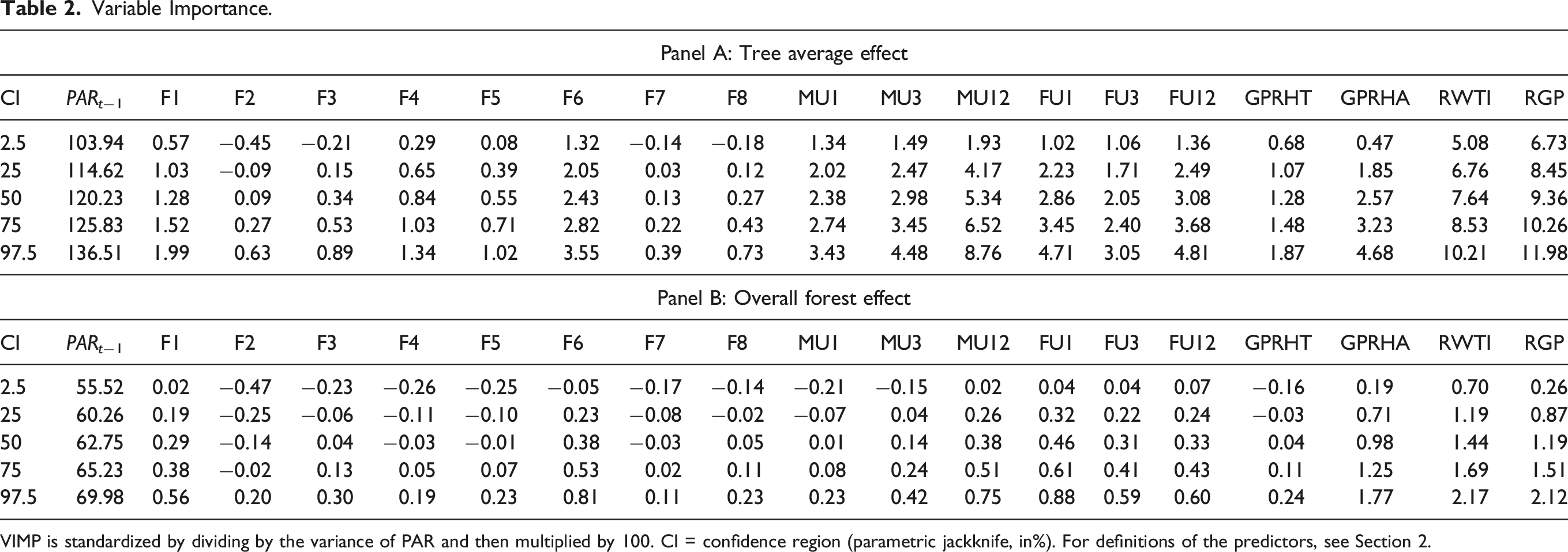
VIMP is standardized by dividing by the variance of PAR and then multiplied by 100. CI = confidence region (parametric jackknife, in%). For definitions of the predictors, see Section 2.

In Table 3, we look at the forecasting properties of real gasoline prices. To this end, we compare a benchmark model, PAR_t+1 = f(PAR_t, CV_t), with a rival model, PAR_t+1 = f(PAR_t, CV_t, RGP_t), both estimated by means of random forests. We estimate the models recursively, using an initial training period of 10 years,¹³ and use the recursive estimates to compute out-of-sample one-month-ahead forecasts of the presidential approval ratings. We then compute the root-mean-squared forecasting error (RMSFE) and the mean absolute forecasting error (MAFE) for both models. The RMSFE (MAFE) ratios inform about the relative forecasting performance of the two competing models. A RMSFE (MAFE)

> 1

shows that the rival model (the one that features the real gasoline price in its array of predictors) performs better than the benchmark model. The RMSFE and MAFE ratios both take on a value of about 1.03, indicating that real gasoline prices have a moderate positive effect on forecast accuracy.

Table 3.

Forecasting Results.

Statistic	Value
RMSFE ratio	1.0275
MAFE ratio	1.0318
RMSFE ratio (discount factor 0.99)	1.0205
MAFE ratio (discount factor 0.99)	1.0392
RMSFE ratio (discount factor 0.9)	1.0921
MAFE ratio (discount factor 0.9)	1.0764
CW test (p-value)	<0.0001
DM test (loss 1, p-value)	<0.0001
DM test (loss 2, p-value)	0.00019

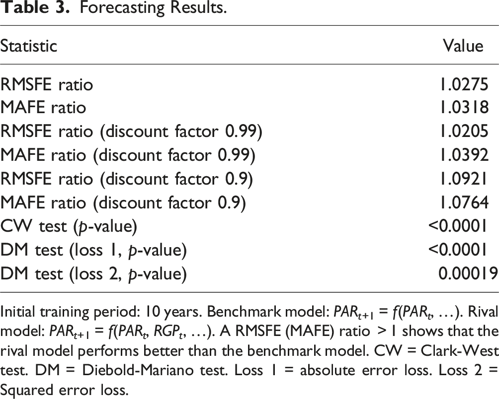
Initial training period: 10 years. Benchmark model: PAR_t+1 = f(PAR_t, …). Rival model: PAR_t+1 = f(PAR_t, RGP_t, …). A RMSFE (MAFE) ratio $> 1$ shows that the rival model performs better than the benchmark model. CW = Clark-West test. DM = Diebold-Mariano test. Loss 1 = absolute error loss. Loss 2 = Squared error loss.

We also report results for a modified RMSFE (MAFE) ratio, where the discount “old” forecast errors using the formula FE_s × γ^T−s, for s = T, T − 1, T − 2, …, where FE denotes the forecast error and T denotes the last observation of the sequence of out-of-sample forecasts. We consider two cases: γ = 0.99 and γ = 0.9. In both cases, more recent forecast errors receive a larger weight as compared to more distant forecast errors. We observe that discounting increases the ratios. This observation suggests that the impact of real gasoline prices on forecast accuracy has tended to increase in the more recent past.

In order to inspect this observation from a different angle, we plot in Figure 4 how the rank of real gasoline price among the predictors changes when we move the end of the recursive-estimation window forward in time. We plot the rank of real gasoline prices in terms of how often this predictor is used for splitting when growing a random forest (upper panel) and in terms of VIMP (lower panel). A lower rank means that real gasoline prices are more important. The evolution of both metrics shows that the importance of real gasoline prices has increased over time.

Figure 4.

Importance of real gasoline prices over time. The rank of RGP in terms of how often this predictor is used for splitting when growing a random forest (upper panel) and in terms of VIMP (lower panel). Window = Index of recursive-estimation window.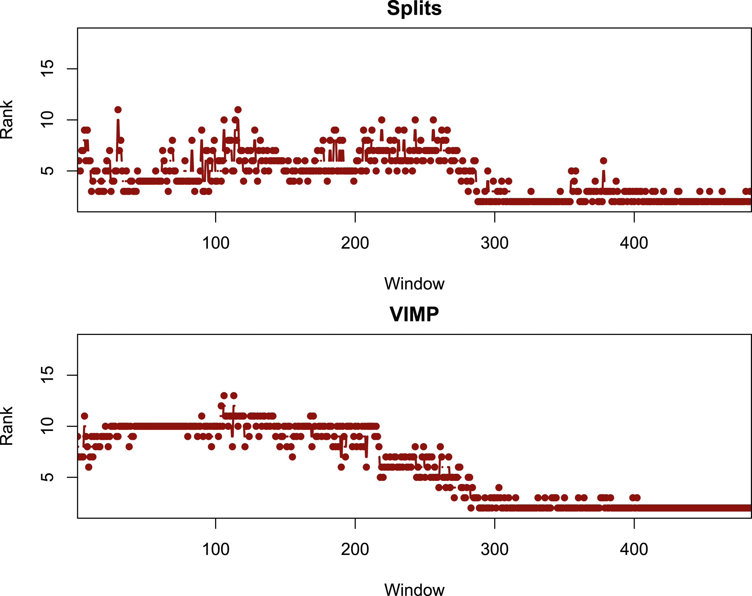

To assess the statistical significance of the impact of real gasoline prices on forecast accuracy, we report, also in Table 3, the results of the Clark and West (2007) and the Diebold and Mariano (1995) tests, where we report results for absolute and squared forecast errors in case of the latter. We report results for both tests because a comparison forecasting models in terms of statistical tests is complicated by the nonlinear and complex structure of random forests. The nonlinear and complex structure of random forests implies that the models are not simple nested versions of each other. In any case, both tests yield statistically significant results and, thus, point in the same direction that real gasoline prices help to improve the accuracy of one-month-ahead forecasts of the presidential approval ratings.

Besides the expectations of the consumers (which have been closely associated with the PAR of the US recently by Gordon (2024)) and businesses captured by the survey data, that forms part of the large database from which the eight factors are extracted, the macroeconomic and financial uncertainties that we include in our array of predictors can be interpreted as forward-looking variables as they capture the non-predictable component of these variables due to various types of shocks (Ludvigson et al., 2021), including those emanating from the energy sector (Sheng et al., 2020), and, as such, account for the sociotropic argument that movements in gasoline prices have a substantial impact on voters expectations of the overall macroeconomy. The incremental impact of real gasoline prices on the presidential approval ratings, therefore, can be interpreted as direct evidence of the pocketbook mechanism.¹⁴ In order to strengthen this interpretation further, we let subsequent macroeconomic conditions, M_t+1, be linked to voters’ expectations of the overall macroeconomy, $M_{t | t + 1}^{e}$ , by some function, $M_{t + 1} = h (M_{t | t + 1}^{e})$ . We also assume, in line with the sociotropic mechanism, that voters’ expectations are some function, g(.), of currently observed real gasoline prices, $M_{t | t + 1}^{e} = g (R G P_{t})$ . We then have $M_{t + 1} = h (g (R G P_{t})) \equiv \tilde{g} (R G P_{t})$ or $R G P_{t} = {\tilde{g}}^{- 1} (M_{t + 1})$ , assuming the usual regularity conditions. If so, real gasoline prices should impact the presidential approval ratings only because current real gasoline prices are a proxy of subsequent macroeconomic conditions. Now, we let the latter be captured by the macroeconomic factors, F1, F2,…,F8, and then include the array of predictors of our random-forests models to include F1_t+1, F2_t+1,…,F8_t+1. If we find a direct impact of RGP_t on the presidential approval ratings in such an extended model, we interpret such a finding as further evidence in support of the pocketbook mechanism. Figure 5 summarizes the results for such an extended model, where we focus again on a the ranking of real gasoline prices. The findings closely resemble the results we plot in Figure 4. Hence, including the lead macroeconomic factors in the array of predictors does not change the overall picture, lending further support to the pocketbook mechanism.¹⁵

Figure 5.

Importance of real gasoline prices over time in an extended model. The rank of RGP in terms of how often this predictor is used for splitting when growing a random forest (upper panel) and in terms of VIMP (lower panel). Window = Index of recursive-estimation window. The extended model features the leads of the macroeconomic factors as additional predictors.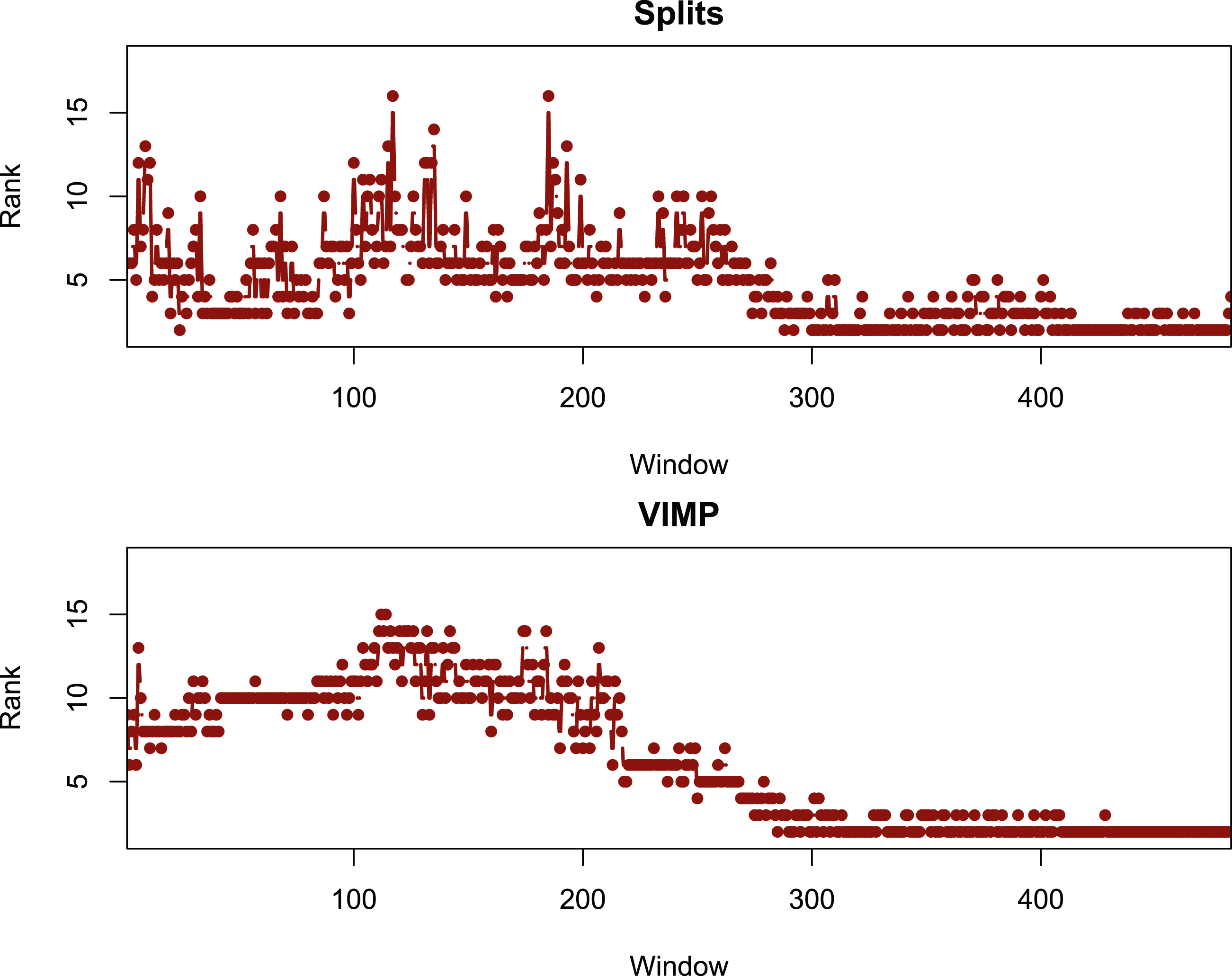

Concluding Remarks

We have used random forests to study the link between the U.S. presidential approval ratings and real gasoline prices, where we have controlled for a large number of control variables that have been studied in earlier literature. Our empirical results have shown that the link between the presidential approval ratings and real gasoline prices is negative and nonlinear. We have found that, putting the lagged presidential approval ratings aside, real gasoline prices clearly are as important, or even more important, than other conventional predictors of the presidential approval ratings. We also observe that real gasoline prices even have predictive value for the subsequent presidential approval ratings in an out-of-sample forecasting experiment. Given the importance of the issue, the predictive value of real gasoline prices for the subsequent presidential approval ratings should be investigated in future research in a more systematic way by considering longer forecast horizons and alternative forecasting models.

Random forests have the advantage that they render it possible to consider a large number of predictors of the the presidential approval ratings, the link of which to the predictors is then traced out in a flexible and completely data-driven way. If voters use real gasoline prices as a source of information about the health of the macroeconomy, then the link between real gasoline prices and the presidential approval ratings should disappear, or at least weaken, once we control for predictors that somehow control for the uncertainty and expectations of the voters about subsequent macroeconomic developments. To this end, we have included in our model various macroeconomic uncertainties and (lead) macroeconomic factors. In spite of the fact that random forests can use these predictors, we have found a direct effect of real gasoline prices on the presidential approval ratings. Our empirical findings, thereby, support the pocketbook mechanism, which stipulates that the link between the the presidential approval ratings and real gasoline prices reflects a sizable effect of the latter on personal economic situations of voters.

At this stage, it is important to point out that our finding that real gasoline prices carry predictive information for the US presidential approval ratings might carry only limited policy implications, given that US presidents cannot necessarily control energy prices, as they are determined by condition worldwide supply and demand. In other words, though chances of being re-elected is likely to be influenced, besides other macroeconomic factors, by real gasoline prices, the president might not be able to do much beyond possibly reducing taxes to compensate for the increase in real gasoline prices at the domestic-level, and/or reducing import tariffs from a global (import) perspective. Having said this, perhaps our results make a case for more emphasis on transition to renewable energy to reduce dependence on gasoline (fossil fuel) and, hence, enhance the probability of retaining the presidential office, besides meeting environmental standards required for achieving the long-term goal of a more “green economy”.

Footnotes

Author’s Note

We would like to thank an anonymous referee for many helpful comments. The usual disclaimer applies.

Declaration of Conflicting Interests

The author(s) declared no potential conflicts of interest with respect to the research, authorship, and/or publication of this article.

Funding

The author(s) received no financial support for the research, authorship, and/or publication of this article.

ORCID iD

Christian Pierdzioch

Notes

Appendix

Figure A1.

Results for a quantile-on-quantile regression.

Figure A2.

Results for wavelet localized multiple correlation.

References

Adrangi

Macri

(2019). Does the misery index influence a U.S. president’s political re-election prospects? Journal of Risk Financial Management, 12(1), 22. https://doi.org/10.3390/jrfm12010022

Bai

Perron

(2003). Computation and analysis of multiple structural change models. Journal of Applied Econometrics, 18(1), 1–22. https://doi.org/10.1002/jae.659

Baumeister

Kilian

Lee

T. K.

(2017). Inside the crystal ball: New approaches to predicting the gasoline price at the pump. Journal of Applied Econometrics, 32(2), 275–295. https://doi.org/10.1002/jae.2510

Berlemann

Enkelmann

(2014). The economic determinants of U.S. presidential approval: A survey. European Journal of Political Economy, 36(1), 41–54. https://doi.org/10.1016/j.ejpoleco.2014.06.005

Berlemann

Enkelmann

Kuhlenkasper

(2015). Unraveling the relationship between presidential approval and the economy: A multidimensional semiparametric approach. Journal of Applied Econometrics, 30(3), 468–486. https://doi.org/10.1002/jae.2380

Bouri

Gupta

Pierdzioch

(2024). Modeling the presidential approval ratings of the United States using machine-learning: Does climate policy uncertainty matter? European Journal of Political Economy, 85(C), 102602. https://doi.org/10.1016/j.ejpoleco.2024.102602

Breiman

(2001). Random forests. Machine Learning, 45(1), 5–32. https://doi.org/10.1023/a:1010933404324

Breiman

Friedman

J. H.

Oshen

Stone

(1984). Classification and regression trees. Chapman and Hall.

Brock

W. A.

Scheinkman

J. A.

Dechert

W. D.

LeBaron

(1996). A test for independence based on the correlation dimension. Econometric Reviews, 15(3), 197–235.

10.

Burden

B. C.

Mughan

(2003). The international economy and presidential approval. Public Opinion Quarterly, 67(4), 555–578. https://doi.org/10.1086/378963

11.

Caldara

Iacoviello

(2022). Measuring geopolitical risk. American Economic Review, 112(4), 1194–1225. https://doi.org/10.1257/aer.20191823

12.

Campbell

J. Y.

(2008). Viewpoint: Estimating the equity premium. Canadian Journal of Economics, 41(1), 1–21. https://doi.org/10.1111/j.1365-2966.2008.00453.x

13.

Chen

Huang

Wang

(2023). Presidential economic approval rating and the cross-section of stock returns. Journal of Financial Economics, 147(1), 106–131. https://doi.org/10.1016/j.jfineco.2022.10.004

14.

Choi

S.-W.

James

Olson

(2016). Presidential approval and macroeconomic conditions: Evidence from a nonlinear model. Applied Economics, 48(47), 4558–4572. https://doi.org/10.1080/00036846.2016.1161718

15.

Chong

Halcoussis

Phillips

(2011). Does market volatility impact presidential approval? Journal of Public Affairs, 11(4), 387–394. https://doi.org/10.1002/pa.410

16.

Clark

T. E.

West

K. D.

(2007). Approximately normal tests for equal predictive accuracy in nested models. Journal of Econometrics, 138(1), 291–311. https://doi.org/10.1016/j.jeconom.2006.05.023

17.

Coggin

T. D.

(2024). U.S. Presidential approval and the macroeconomy: 1960−2022. Economics and Politics, 37(1), 376–399. https://doi.org/10.1111/ecpo.12322

18.

Dickerson

(2016). Economic perceptions, presidential approval, and causality: The moderating role of the economic context. American Politics Research, 44(6), 1037–1065. https://doi.org/10.1177/1532673x15600787

19.

Diebold

F. X.

Mariano

R. S.

(1995). Comparing predictive accuracy. Journal of Business and Economic Statistics, 13(3), 253–263. https://doi.org/10.1080/07350015.1995.10524599

20.

Fauvelle-Aymar

Stegmaier

(2013). The stock market and U.S. presidential approval. Electoral Studies, 32(3), 411–417. https://doi.org/10.1016/j.electstud.2013.05.024

21.

Fernández-Macho

(2018). Time-localized wavelet multiple regression and correlation. Physica A: Statistical Mechanics and its Applications, 492(C), 1226–1238. https://doi.org/10.1016/j.physa.2017.11.050

22.

Fiorina

M. P.

(1981). Retrospective voting in American politics. Yale University Press.

23.

Gomez

B. T.

Wilson

J. M.

(2001). Political sophistication and economic voting in the American electorate: A theory of heterogeneous attribution. American Journal of Political Science, 45(4), 899–914. https://doi.org/10.2307/2669331

24.

Gordon

R. J.

(2024). How do electoral votes, presidential approval, and consumer sentiment respond to economic indicators? National Bureau of Economic Research (NBER). Working Paper No. 33068.

25.

Gupta

Kanda

P. T.

Wohar

M. E.

(2021). Predicting stock market movements in the United States: The role of presidential approval ratings. International Review of Finance, 21(1), 324–335. https://doi.org/10.1111/irfi.12258

26.

Gupta

Wohar

M. E.

(2017). Forecasting oil and stock returns with a Qual VAR using over 150 years off data. Energy Economics, 62(C), 181–186. https://doi.org/10.1016/j.eneco.2017.01.001

27.

Halcoussis

Lowenberg

A. D.

Phillips

G. M.

(2009). The Obama effect. Journal of Economics and Finance, 33(3), 324–329. https://doi.org/10.1007/s12197-009-9077-3

28.

Harbridge

Krosnick

J. A.

Wooldridge

J. M.

(2016). Presidential approval and gas prices: Sociotropic or pocketbook influence? In Krosnick

J. A.

Chiang

I.-C. A.

Stark

T. H.

(Eds.), Political psychology: New explorations (pp. 246–275). Taylor and Francis.

29.

Hastie

Tibshirani

Friedman

(2009). The elements of statistical learning: Data mining, inference, and prediction (Vol. 2). Springer.

30.

Iseringhausen

Petrella

Theodoridis

(2023). Aggregate skewness and the business cycle. https://doi.org/10.1162/rest_a_01390

31.

Ishwaran

Kogalur

U. B.

(2023). Fast unified random forests for survival, regression, and classification (RF-SRC). R package version 3.2.2. https://www.randomforestsrc.org/

32.

Jurado

Ludvigson

S. C.

(2015). Measuring uncertainty. American Economic Review, 105(3), 1177–1216. https://doi.org/10.1257/aer.20131193

33.

Kilian

(2010). Explaining fluctuations in U.S. Gasoline prices: A joint model of the global crude oil market and the U.S. retail gasoline market. Energy Journal, 31(2), 87–104.

34.

Kilian

Zhou

(2022). Oil prices, gasoline prices and inflation expectations. Journal of Applied Econometrics, 37(5), 867–881. https://doi.org/10.1002/jae.2911

35.

Kim

S. E.

Yang

(2022). Gasoline in the voter’s pocketbook: Driving times to work and the electoral implications of gasoline price fluctuations. American Politics Research, 50(3), 312–319. https://doi.org/10.1177/1532673x211043445

36.

Kinder

D. R.

Kiewiet

D. R.

(1981). Sociotropic politics: The American case. British Journal of Political Science, 11(2), 129–161. https://doi.org/10.1017/s0007123400002544

37.

Kramer

G. H.

(1971). Short-term fluctuations in U.S. voting behavior, 1896−1964. American Political Science Review, 65(1), 131–143. https://doi.org/10.2307/1955049

38.

Ludvigson

S. C.

(2021). Uncertainty and business cycles: Exogenous impulse or endogenous response? American Economic Journal: Macroeconomics, 13(4), 369–410. https://doi.org/10.1257/mac.20190171

39.

Ludvigson

S. C.

(2009). Macro factors in bond risk premia. Review of Financial Studies, 22(12), 5027–5067. https://doi.org/10.1093/rfs/hhp081

40.

Ludvisgon

S. C.

(2011). A factor analysis of bond risk premia. In Ulah

Giles

(Eds.), Handbook of empirical economics and finance (pp. 313–372). Chapman and Hall.

41.

Pástor

Veronesi

(2020). Political cycles and stock returns. Journal of Political Economy, 128(11), 4011–4045. https://doi.org/10.1086/710532

42.

R Core Team . (2023). R: A language and environment for statistical computing. R Foundation for Statistical Computing. https://www.R-project.org/

43.

Sheng

Gupta

(2020). The impacts of structural oil shocks on macroeconomic uncertainty: Evidence from a large panel of 45 countries. Energy Economics, 91(C), 104940. https://doi.org/10.1016/j.eneco.2020.104940

44.

Sim

Zhou

(2015). Oil prices, US stock return, and the dependence between their quantiles. Journal of Banking and Finance, 55(C), 1–8. https://doi.org/10.1016/j.jbankfin.2015.01.013

Gasoline Prices and Presidential Approval Ratings of the United States

Abstract

Keywords

Introduction

Data

Random Forests

Empirical Results

Concluding Remarks

Footnotes

Author’s Note

Declaration of Conflicting Interests

Funding

ORCID iD

Notes

Appendix

References