Sage Journals: Discover world-class research

Abstract

Chitosan nanofibers reinforced with tungsten disulfide inorganic nanotubes (INT-WS₂) were fabricated in this study. The aim was to investigate the effect of the material parameters and the electrospinning process parameters on the obtained nanofibrous morphology of the mats. The INT-WS₂ content, the polymer solution concentration, the electric field strength, and the solution's flow rate were the investigated factors within the framework of response surface methodology. Scanning electron microscopic and image analysis were used for the dimensional characterization of the nanofibrous morphology and the estimation of three selected responses. Two responses were related to the quality of the nanofibrous morphology: the number surface density of the beads (N_bead) and the average bead-to-fiber diameter (D_bead/D_fiber). The third response was indicative of the fiber thickness (D_fiber). The developed models as well as the coupling and the individual effects of the four investigated factors are given. The results indicate that the electrospun nanofibrous morphology is mostly affected by the polymer solution concentration, the electric field strength and the INT-WS₂ loading. Furthermore, the response-surface results reveal possible experimental pathways that may be followed in order to obtain specified nanofibrous chitosan/INT-WS₂ morphologies.

Keywords

Nanofiber chitosan electrospinning design of experiments tungsten disulfide

Introduction

Nowadays, there are many different techniques for the production of highly porous polymeric structures. Most common of them include particle leaching [1], phase separation [2], freeze drying [3], rapid prototyping [4], CO₂ foaming and antisolvent techniques [5], co-continuous blends [6], and fiber- or textile-forming processes [7]. Electrospinning is an attractive technique for the production of highly porous and fibrous structures [8,9]. These fibrous materials have been successfully used in the membrane/filtration technology [10,11] and biomedical applications [12,13]. Moreover, electrospinning, compared to other techniques, has many advantages such as high production yield, low cost, and the simplicity of the process [14]. The fiber diameters that can be produced by electrospinning may vary from a few nanometers to a few micrometers.

The electrospun morphology is affected by several material and processing parameters. The main material parameters that affect the electrospun fibrous morphology are the solution concentration, dynamic viscosity, density, surface tension, dielectric permittivity, and electrical conductivity. The aforementioned factors, in turn, depend on the type of polymer, solvent, or the filler used. At the same time, the electrospun fibrous morphology also depends on the electrospinning process parameters: the electric field, the diameter and the angle of the spinneret, the spinning distance, and the flow rate [15]. It has been reported that the fiber diameter decreases by a polymer solution concentration decrease, surface tension decrease, solution viscosity decrease, solution conductivity increase, and field strength increase [16]. However, regarding the effect of the applied voltage, contradictory experimental findings exist in the literature. The fine tuning of the fibrous morphology can be achieved by appropriately adjusting the electrospinning parameters [17]. Consequently, the impact of the processing and material parameters on the resulting electrospun morphology is significant from both theoretical and practical point of view.

As mentioned earlier, very thin fibers with nanoscaled diameters (nanofibers) can be produced via electrospinning. These nanofibrous structures bring new opportunities with respect to the material properties that can be achieved: high surface-to-volume ratio and significantly high porosity. Nanofibers cover a broad range of current and emerging technological applications. These applications include tissue engineering, anti-microbiological wound dressings [18], adsorption/filtration [10], drug delivery [12], catalysis [19], and sensors [20]. For the effective development and commercialization of the electrospun mats there need to be considered not only the fibrous structure itself but also the beads, which often occur in the fibrous structure. Even though beads are regarded as nondesirable characteristics (“byproducts”) of the fibrous structure, they can have functional roles in various applications. For instance, the beads on the electrospun fibrous structure can be used for cell inclusion or drug reservoirs [21], while the formation beaded fibers was found to promote hydrophobicity [22]. In many of the aforementioned applications, the biodegradability and the biocompatibility of the polymer should be considered. Chitosan is a biodegradable and biocompatible carbohydrate polymer with the ability to form nanofibers via electrospinning [23 –25]. Electrospinnable chitosan solutions have been prepared using various solvents such as aqueous acetic acid [24 –28], trifluoroacetic acid, and trifluoroacetic acid/dichloromethane mixtures [29,30]. Aqueous acetic acid should be the preferred solvent in the case of large-scale chitosan nanofiber production due to its low cost and reduced environmental and health considerations compared to the rest of the aforementioned solvents [31]. However, difficulties in obtaining uniform chitosan nanofibers from aqueous acetic acid solutions have been reported [30 –32]. These difficulties arise from various factors such as the relatively high molecular weight of chitosan, the reduced stability of the aqueous acetic acid solution, and the repulsive forces between the ionic groups within the backbone of chitosan [33]. At the same time, there are various types of commercial chitosan (food grade, medical grade, etc.) that vary with respect to their physiochemical characteristics (molecular weight, deacetylation degree, viscosity, origin, etc.). The electrospinnability of the different types of chitosan, using aqueous acetic acid solutions, may vary considerably. There is also some divergence in the morphology of the resulting electrospun film, when different types of chitosan are used. In that sense, the electrospinning parameters for the formation of chitosan nanofibers should be reconsidered, as far as the different types of chitosan are concerned.

Nanocomposite nanofibers have attracted much attention lately, due to the significant enhancement in the mechanical and other properties of the nanofibers [34,35]. Several nanofillers can be used as reinforcements for the production of nanocomposite nanofibers depending on the targeted application. In the case of chitosan, multiwall carbon nanotubes (MWCNTs) [36], hydroxyapatite [37], mesoporous silica [38], silver nanoparticles [32], and chitin nanocrystals [39] have been used. However, studies dealing with chitosan nanocomposites that incorporate other types of novel inorganic nanofillers and especially nanotubes (e.g. inorganic nanotubes) are still missing. Tungsten disulfide inorganic nanotubes (INT-WS₂) combine a variety of attractive physiochemical properties such as biocompatibility, high Young's modulus, compressive strength, and chemical inertness. INT-WS₂ exhibit high aspect ratio, with diameter around 20 nm and length up to a few microns [40 –42]. Therefore, the continuation of the research efforts aiming at the nanoreinforcement of chitosan nanofibers with controlled morphology may expand their use to new applications and products.

Many studies regarding the electrospinning of chitosan and other biopolymers [28,43] investigate the effect of the electrospinning parameters on the fiber diameter, by modifying one factor at a time, while maintaining the other factors constant. Another method commonly used is the best-guess method, which is based on experience. Both of these methods have major disadvantages. The study of the electrospinning process with either method is not quantitatively accurate and systematic. At the same time, the best combination of factors and responses cannot be found, since interactions between factors cannot be detected. These limitations are even more pronounced when many factors and responses are investigated. There is an ongoing research activity regarding the applicability of design of experiments (DoE) in the electrospinning process. In order to identify the significant variables of the system, significant research efforts aim at the development of suitable experimental designs [21,44]. DoE systematically applies statistical methods, such as replication, blocking and randomization, to experimental procedures in order to ensure the accuracy of the model formed. Response surface methodology (RSM) can shed light to the interactions between the variables (factors) of the system. Moreover, RSM provides the possibility to quantify these interactions. It has been established that RSM is a reliable methodology which can be applied in various systems/processes found in academic research and industry [45]. Last but not the least, compared to other traditional methods RSM is less time consuming because, for a certain number of factors within specified ranges, RSM uses the minimum number of experimental runs [46].

In this work, a novel polymer–nanotube nanocomposite system in the form of nanofibrous membrane was investigated. Chitosan nanofibrous membranes, reinforced with INT-WS₂, were prepared by electrospinning using DoE. The experimental design was employed for the following purposes: (a) the identification and quantification of process and material parameters that significantly affect the final electrospun chitosan/INT-WS₂ nanofibrous morphology, (b) the identification and quantification of the interactions between these parameters, (c) the revelation of possible pathways in order to obtain nanocomposite and nanofibrous films with specified morphologies.

Experimental section

Materials

Medical grade chitosan (95/500) with high deacetylation degree (≥92.6%) was purchased from Heppe Medical Chitosan GmbH (Germany). According to the product's datasheet, the molecular weight of this type of chitosan is 200–400 kDa, as determined by gel permeation chromatography (GPC). Acetic acid (100%, anhydrous) was purchased from Merck (Germany), while INT-WS₂ were purchased form Nanomaterials Ltd. (Israel). The aforementioned materials were used as received, without any further treatment.

Preparation of the nanocomposite electrospun mats

Initially, chitosan/INT-WS₂ solutions, needed for the electrospinning process, were prepared. Specified INT-WS₂ content (0.5–1% w/v) was dispersed in aqueous acetic acid (90% acetic acid/10% water v/v) by sonicating the solution for 10 min. Relatively low chitosan loadings (2.5–3.5% w/v) were then added in the solution and it was subsequently sonicated for another 5 min. In the case of chitosan-only solution preparation the first step of the procedure (sonication for 10 min) was omitted. The (nanocomposite) chitosan solution was stirred overnight (for 14h minimum) until homogenous solution was received. The (nanocomposite) chitosan solution was then poured into a glass syringe, having 10 mL internal volume. A 20G needle (with 0.9 mm outer diameter) was firmly attached to the syringe. A Qis Ν1000 syringe pump was used to inject polymer solution with controllable flow rate (between 0.5 and 1.5 mL/h). A Spellman CZE 1000R high voltage supply was used for the generation of electric field between the needle and the grounded collector. The collector was consisting of a metal plate covered with an aluminum foil. The needle was connected to the high voltage supply, having a positive charge (+), and the grounded electrode (-) was attached to the metal target. The needle-collector distance was set to 10 cm, while the voltage varied between 20 kV and 26kV. After the preparation of chitosan/INT-WS₂ electrospun mats, all samples were dried in vacuum overnight at room temperature. The custom electrospinning setup used for the production of nanofibers is shown in Figure 1. It is worth noting that the electrospinning setup was enclosed inside a chamber so as to maintain a stable environment during the electrospinning process. It has been reported that high relative humidity (%RH) alterations may significantly affect the electrospun morphology due to conductivity fluctuations [44,47]. In our case, all electrospinning experiments were carried out at controlled room temperature (23.4–25.1℃) and ambient relative humidity (30–35%).

Figure 1.

A schematic representation of the electrospinning apparatus used.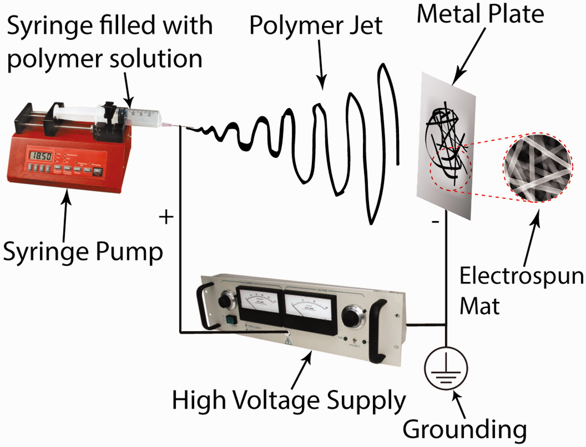

Experimental design and responses

A D-optimal experimental design was used, with an initial condition number equal to 8.37 (<10) and objective response-surface modeling. This experimental design included 29 experimental runs. Four of these runs were pure replicates. Each one of the 29 experimental runs was executed once. The flow rate (qualitative factor), the solution concentration (quantitative factor), the INT-WS₂ loading (quantitative factor) and the electric field strength (voltage/length unit - quantitative factor) were selected as controllable factors. In this case, the flow rate was considered qualitative factor, due to the fact that the experimental setup used allows the flow rate to be defined only at specified levels. In Table 1, the factor settings used in the experimental design, are shown.

Table 1.

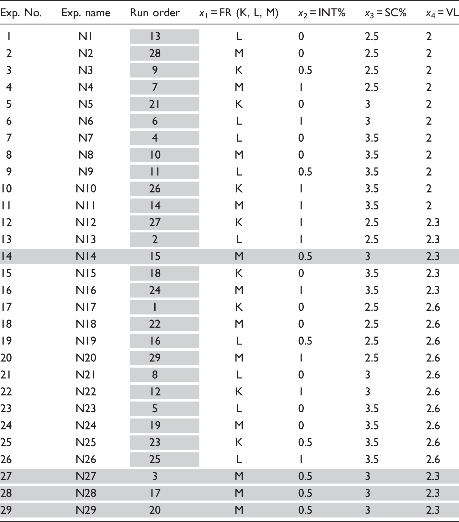
Experimental conditions for the electrospinning of chitosan/INT-WS₂ nanocomposites.

Controllable factors	Factor levels
Flow rate (FR)	K, L, M
INT-WS₂ loading (INT%)	0, 0.5, 1 (%w/v)
Solution concentration (SC%)	2.5, 3, 3.5 (%w/v)
Electric field strength (VL)	2, 2.3, 2.6 (kV/cm)

K = 0.5 mL/h, L = 1 mL/h, M = 1.5 mL/h.

In addition to the parameters (factors) already included in this experimental design, some extra material and process parameters could affect the morphology of chitosan/INT-WS₂ nanocomposite nanofibers. Specifically, solution's conductivity, surface tension, target characteristics (e.g. the rotational speed of a rotating target), ambient conditions (i.e. elevated temperatures, different inert gases, etc.) could be considered. However, the incorporation of many different factors would render the experimental design rather complicated and nonexploitable from a practical point of view. This is attributed to the fact that it is not economical and sometimes not feasible to measure and control so many experimental parameters simultaneously in the industrial scale.

It is worth noting that the levels and the limits of each factor were carefully selected based on some preliminary (screening) experiments. In brief, at solution concentrations lower than 2.5% (w/v) only beads (at 1% w/v) or mostly beads rather than fibers (at 2% w/v) were formed. This denoted that solution concentrations higher than 2.5% (w/v) are required in order to obtain well-formed nanofibers. Nevertheless, solutions with chitosan concentrations higher than 3.5 % (w/v) were too viscous and not electrospinnable. The INT-WS₂ loading was kept at relatively low values (up to 1% w/v) since the viscosity of the solution significantly increases at higher INT-WS₂ concentrations, which hinders the electrospinnability of the solution. On the other hand, a 2–2.6 kV/cm electric field strength range was selected for two reasons. Firstly, no or very few nanofibers were deposited on the grounded target at electric field strength values lower than 2 kV/cm. Secondly, the occurrence of many electrical discharges and sparks at electric field strength values higher than 2.6 kV/cm prevented the control of the electrospinning process. The flow rate was set in the range 0.5–1.5 mL/h. At flow rates lower than 0.5 mL/h solidification of the chitosan solution inside the needle (clogging) was observed. Deposition of a thick chitosan film on the target was observed at flow rates higher than 1.5 mL/h due to insufficient time left for solvent evaporation and fiber consolidation.

The experimental parameters represent the vertices of a three-dimensional (3D) cubic region (design space), which is formed by combining the upper and the lower limits of each factor. The different experimental runs are set as discernible points in the design space, according to our experimental design. For better clarification, the experimental runs are presented on a separate cube for each level (K, L, M) of flow rate (Figure 2). The design space is represented by this cubic region, so as the experiments will yield not only adequate but also reliable measurements of the responses of interest. For a quadratic model, the experiments must be carried out for at least three levels of each factor. These levels are best chosen equally spaced (e.g. −1, 0, + 1).

Figure 2.

The 3D experimental space. The numbered green spheres on the vertices of the cube correspond to the experimental runs listed in Table 2. For each level (K,L,M) of flow rate the experimental runs are presented on a separate cube, in order to offer a clearer representation.

In Table 2, the conditions of the 29 experimental run are summarized. These 29 experimental runs were carried out randomly in order to ensure randomization, while four of these runs were replicates to ensure replication. Moreover, three responses were determined in order to obtain a more reliable representation of the experimental results. The selected responses were used in the statistical analysis in order to consider not only the fibrous but also the beaded structures of the resulting electrospun mats. However, only the fibrous fraction of the electrospun mat is taken into consideration in most published studies, while the beaded structures are often neglected. Therefore, we seek to obtain a comprehensive and complete picture of the electrospun mats' morphology by introducing the following three responses: the fiber diameter (D_fiber), the number surface density of the beads (N_bead), and the bead-to-fiber diameter (D_bead/D_fiber). D_fiber is related to the fiber thickness, while the rest of the responses (N_bead and D_bead/D_fiber) were introduced in order to investigate the formation of beaded structures on the produced electrospun mats. A comprehensive description of the experimental workflow and the analysis of the results, in the framework of the design of experiments, are given in Figure 3.

Table 2.

The design of experiments being used consisted of 29 runs. The two fundamental principles of design of experiments (randomization and replication), are highlighted.

Exp. No.	Exp. name	Run order	x₁ = FR (K, L, M)	x₂ = INT%	x₃ = SC%	x₄ = VL
1	N1	13	L	0	2.5	2
2	N2	28	M	0	2.5	2
3	N3	9	K	0.5	2.5	2
4	N4	7	M	1	2.5	2
5	N5	21	K	0	3	2
6	N6	6	L	1	3	2
7	N7	4	L	0	3.5	2
8	N8	10	M	0	3.5	2
9	N9	11	L	0.5	3.5	2
10	N10	26	K	1	3.5	2
11	N11	14	M	1	3.5	2
12	N12	27	K	1	2.5	2.3
13	N13	2	L	1	2.5	2.3
14	N14	15	M	0.5	3	2.3
15	N15	18	K	0	3.5	2.3
16	N16	24	M	1	3.5	2.3
17	N17	1	K	0	2.5	2.6
18	N18	22	M	0	2.5	2.6
19	N19	16	L	0.5	2.5	2.6
20	N20	29	M	1	2.5	2.6
21	N21	8	L	0	3	2.6
22	N22	12	K	1	3	2.6
23	N23	5	L	0	3.5	2.6
24	N24	19	M	0	3.5	2.6
25	N25	23	K	0.5	3.5	2.6
26	N26	25	L	1	3.5	2.6
27	N27	3	M	0.5	3	2.3
28	N28	17	M	0.5	3	2.3
29	N29	20	M	0.5	3	2.3

Figure 3.

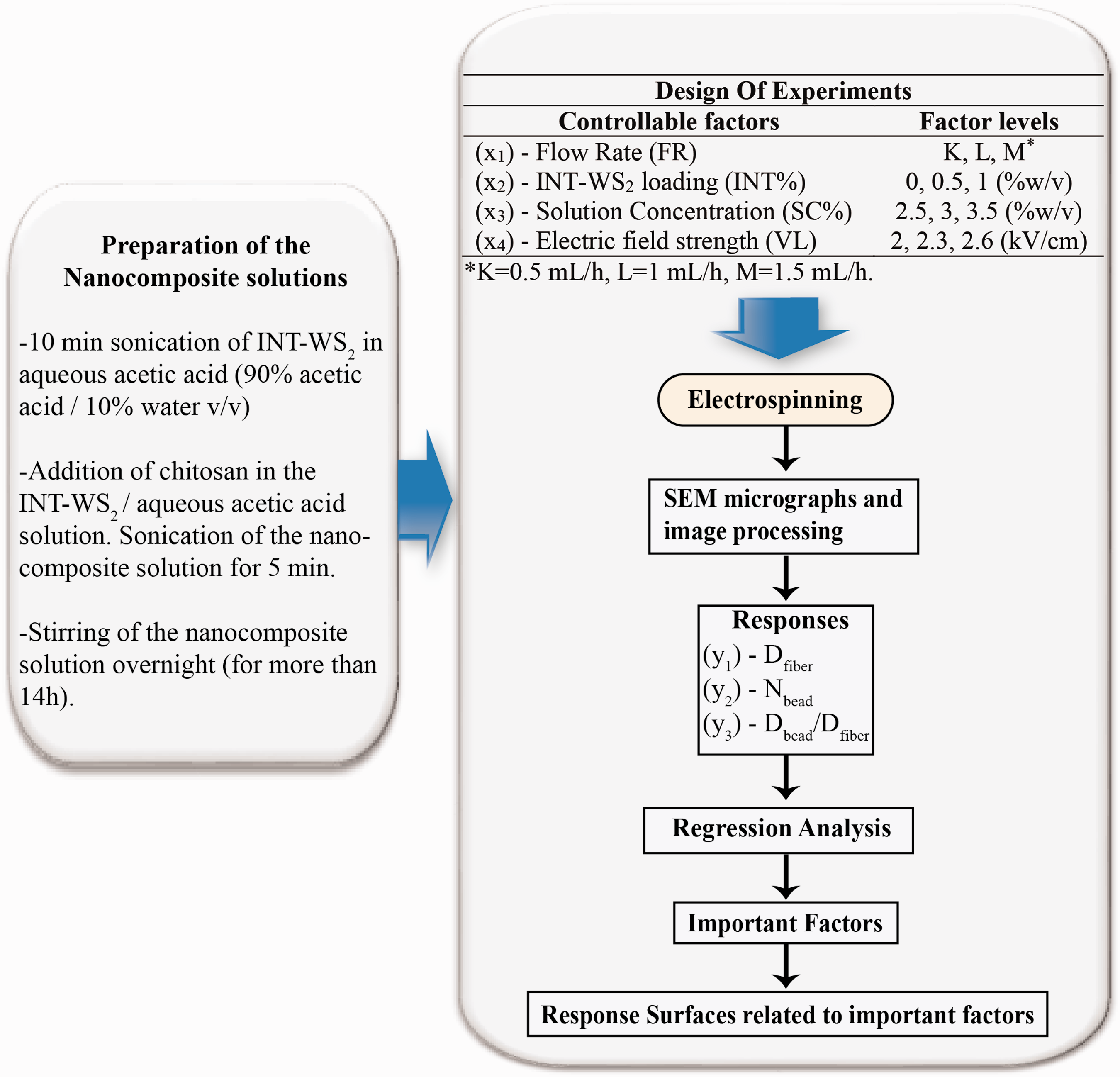
The experimental workflow and the analysis of the results in the framework of the design of experiments methodology.

Morphological characterization and statistical analysis

Morphological examination of the electrospun mats was realized by means of scanning electron microscopy (SEM) using a JEOL 6610LV microscope. The dispersion of INT-WS₂ in chitosan nanofibrous mats was evaluated via energy-dispersive spectroscopy (EDS), using a large area (80 mm²) silicon drift detector (X-Max 80, Oxford Instruments), attached to the SEM. All images and spectra were recorded and analyzed using AZtech Nanoanalysis software (Oxford Instruments). All surfaces were coated with gold prior observation, in order to prevent surface charging under the electron beam, using a Quorum 150R S magnetron sputtering device.

The geometrical characteristics (D_fiber, N_bead and D_bead/D_fiber) of the electrospun mats were measured and quantified using image analysis software (ImageJ 1.50b and BoneJ plug-in for the measurement of D_fiber) [48]. Two samples were examined for each experimental run. At least two indicative areas of each sample were selected, while images of two different magnifications (×10,000 and ×20,000) were recorded from each area. For the determination of the morphological characteristics of the nanofibrous structure (D_fiber, N_bead and D_bead/D_fiber) at least four images were processed. Furthermore, only images of lower magnification (i.e. × 10,000) were used for the number of beads per µm² (N_bead) measurement. In this way, a better N_bead assessment was achieved by taking into account the widest possible area.

For the creation of the D-optimal design and the posterior regression analysis, MODDE 10.0 software was employed. All the figures related to the experimental design and statistical analysis shown in this work, were created using the same software.

Results and discussion

Morphology

The morphology and the diameter of the produced fibers could be partly affected by the elongational flow's aligning effect due to the presence of the electrical field, the polymer solution's surface tension, and the rapid solidification of the fibers [21,44]. During electrospinning, the electrical forces applied make the fibers thinner. However, the surface area of the liquid (polymer solution) is decreased due to the surface tension [49]. Hence, structures, that contain not only fibers but also beads, may be formed in some cases during the solidification of the polymer solution. On the other hand, the polymer solution's flow rate in the syringe may also affect, in some extent, the formation of beads inside the electrospun fibrous structure. In general, the polymer solution in lower flow rates has more time for polarization. Although, in higher flow rates the solvent evaporation time is much shorter and the elongational forces much weaker. Hence, beaded fibers with relatively large diameters may be formed in higher flow rates. It is worth noting that some effects of the parameters mentioned (e.g. applied voltage, flow rate) may have a controversial effect on the electrospun morphology depending on the type of the polymer being used [9,50].

SEM photos of six indicative experimental runs are shown in Figure 4. The produced nanofibrous electrospun mats mainly exhibited four types of morphology which are listed below:

(a) Nanofibers with few (small-sized) beads (Exp. N2 and N23).

(b) Nanofibers with many beads (Exp. N9).

(d) Bead-free nanofibers (Exp. N21).

Figure 4.

SEM photos of six morphologically indicative experimental runs (N2, N4, N9, N21, N23, N28). The scale bar for the × 10,000 photos is set to 3 µm, while for the × 20,000 is set to 1 µm.

When the polymer solution concentration is low, wet fibers cannot be strained by the electrical field upon their deposition on the metal plate. Their solidification procedure is governed by the relaxation process, which depends on the viscoelastic properties, and the surface tension. Τhereby, beaded fibers may occur [21]. The viscosity increase, carried out by increasing the polymer concentration in the solution, could avert the jet collapse and the droplet generation prior to solvent evaporation. Moreover, at higher solution concentrations many entanglements among the polymer chains may occur. In that sense, the solvent's molecules are allocated among the entangled polymer chains and the ability of bead formation is reduced due to the surface tension decrease [51]. However, beaded fibers may also be observed at very high polymer concentrations, due to the increased viscosity of the solution which hinders the straining of the fibers and the solidification of the polymer shortly after its exit from the needle tip.

When the polymer concertation in the solution exceeds a certain (critical) concentration (in our case more than 3% w/v), the fibers were mostly dried upon their deposition on the metal target, so as a rather uniform fibrous mat is obtained. In this case, the number of beads along the fibers decreases. This explains the formation of rather uniform nanofibers for solution concentration 3% w/v (N21), the formation of beaded fibers in concentrations lower than 3% w/v (i.e. 2.5% w/v, N2) and the formation of slightly beaded fibers in high polymer solution concentrations (i.e. 3.5% w/v, N23). However, some other factors may contribute to the bead formation.

With the addition of INT-WS₂ more beads are formed on the nanofibrous structure. This could be ascribed to the fact that the nanotubes may alter locally the conductivity of the polymer solution. These local conductivity alterations could cause electric field inhomogeneity. The electric field inhomogeneity may induce polymer solution to be strained at different rates. Consequently, this may lead to beaded nanofibrous structures. Nevertheless, the formation of beaded nanofibrous structures may also be attributed to the hindering of the polymer chain's entanglements caused by the presence of INT-WS₂. In that sense, the surface tension should increase and more beads are formed. Therefore, the aforementioned explain the production of rather beaded structures in the experimental runs N4, N9, and N28. The dispersion of INT-WS₂ inside the chitosan nanofibrous was investigated by means of EDS elemental analysis (see Supplementary Material). INT-WS₂ appears to be well-dispersed in the fibers and the beads of the electrospun film, with no evident signs of aggregation (Figure S1a and S1b). The values (raw data) and the corresponding error bars of the three responses (D_fiber, N_bead, and D_bead/D_fiber), for the 29 experimental runs, are presented in Figure 5. It is worth noting that the average values of the responses were used in the subsequent regression analysis.

Figure 5.

The values and the corresponding error bars of the three responses (raw data): (a) D_fiber, (b) N_bead, and (c) D_bead/D_fiber), for the 29 experimental runs.

Raw response data assessment and regression analysis

Multiple linear regression analysis (MLR) was performed, in order to assess the impact of each factor on the electrospun nanofibrous morphology and to find possible pathways towards a desired morphology. The raw (as-measured) data of the three responses (y₁≡D_fiber, y₂≡N_bead, y₃≡D_bead/D_fiber) are illustrated in Figure 6(a) to (c). The raw response data distribution appears to be rather unsymmetrical. The respective Box–Whisker plots corroborate the unsymmetrical distribution of the raw response data (Figure 6(d) to (f)). These raw response data need to be transformed, since the data subjected to regression analysis, should follow a normal distribution. Therefore, three different logarithmic transformations were applied to the raw data of each response (y₁, y₂, and y₃), prior conducting MLR. The transformations applied to the raw response data are summarized in Table 3.

Figure 6.

Histograms illustrating the raw data distribution of the three responses: (a) D_fiber, (b) N_bead, (c) D_bead/D_fiber. The corresponding Box–Whisker plots (d,e,f) indicate the unsymmetrical distribution of the raw data.

Table 3.

Responses' transformations and terms used to model each response.

Analysis type: Multiple linear regression (MLR)
Model type: Quadratic (for all responses)
Nontransformed responses	Transformed responses	Model terms	Number of model terms
y₁ ≡ D_fiber	Y₁ = 10log(0.31 × y₁-13)	Constant, INT%, SC%, VL, SC%×SC%, INT%×SC%.	6
y₂ ≡ N_bead	Y₂ = 10log(3.1 × y₂+0.8)	Constant, FR(K), FR(L), FR(M), INT%, SC%, VL, INT% × INT%, SC% × SC%, VL × VL, FR(K) × INT%, FR(L) × INT%, FR(M) × INT%, FR(K) × SC%, FR(L) × SC%, FR(M) × SC%, FR(K) × VL, FR(L) × VL, FR(M) × VL, INT% × SC%, INT% × VL, SC% × VL.	22
y₃ ≡ D_bead/D_fiber	Y₃ = 10log(2 × y₃+12)	Constant, INT%, SC%, VL, INT% × INT%, SC% × SC%, VL × VL, INT% × VL.	8
Full list of model terms that can be introduced in the quadratic model's equation^a		Constant, FR(K), FR(L), FR(M), INT%, SC%, VL, INT% × INT%, SC% × SC%, VL × VL, FR(K) × INT%, FR(L) × INT%, FR(M) × INT%, FR(K) × SC%, FR(L) × SC%, FR(M) × SC%, FR(K) × VL, FR(L) × VL, FR(M) × VL, INT% × SC%, INT% × VL, SC% × VL.	22^b

A quadratic model with four factors can be expressed by the following quadratic equation:

y = β_{0} + β_{1} x_{1} + β_{2} x_{2} + β_{3} x_{3} + β_{4} x_{4} + β_{11} x_{1}^{2} + β_{22} x_{2}^{2} + β_{33} x_{3}^{2} + β_{44} x_{4}^{2} + β_{12} x_{1} x_{2} + β_{13} x_{1} x_{3} + β_{14} x_{1} x_{4} + β_{23} x_{2} x_{3} + + β_{24} x_{2} x_{4} + \in

(1)

where β₀ is a constant, β_ij are the coefficients of the model (with i = 1,2,3,4 and j = 0,2,3,4), x_i are the factors of the model (in our case x₁≡FR, x₂≡INT%, x₃≡SC%, x₄≡VL) and ∈ is the error. As can be seen from equation (1) there are four term types: constant (i.e. β₀), linear (e.g. β₁x₁), quadratic (e.g.

β_{11} x_{1}^{2}

), and interaction terms (e.g. β₁₂x₁x₂).

The initial number of model terms that can be introduced in the equation is 14 according to equation (1). However, the flow rate (FR) here is considered as a qualitative factor. In that sense, additional terms [FR(K), FR(L), FR(M), FR(K) × INT%, FR(L) × INT%, FR(M) × INT%, FR(K) × SC%, FR(L) × SC%, FR(M) × SC%, FR(K) × VL, FR(L) × VL, FR(M) × VL] for each discrete level (K,L,M) of FR were introduced in equation (1) making a total of 22 terms.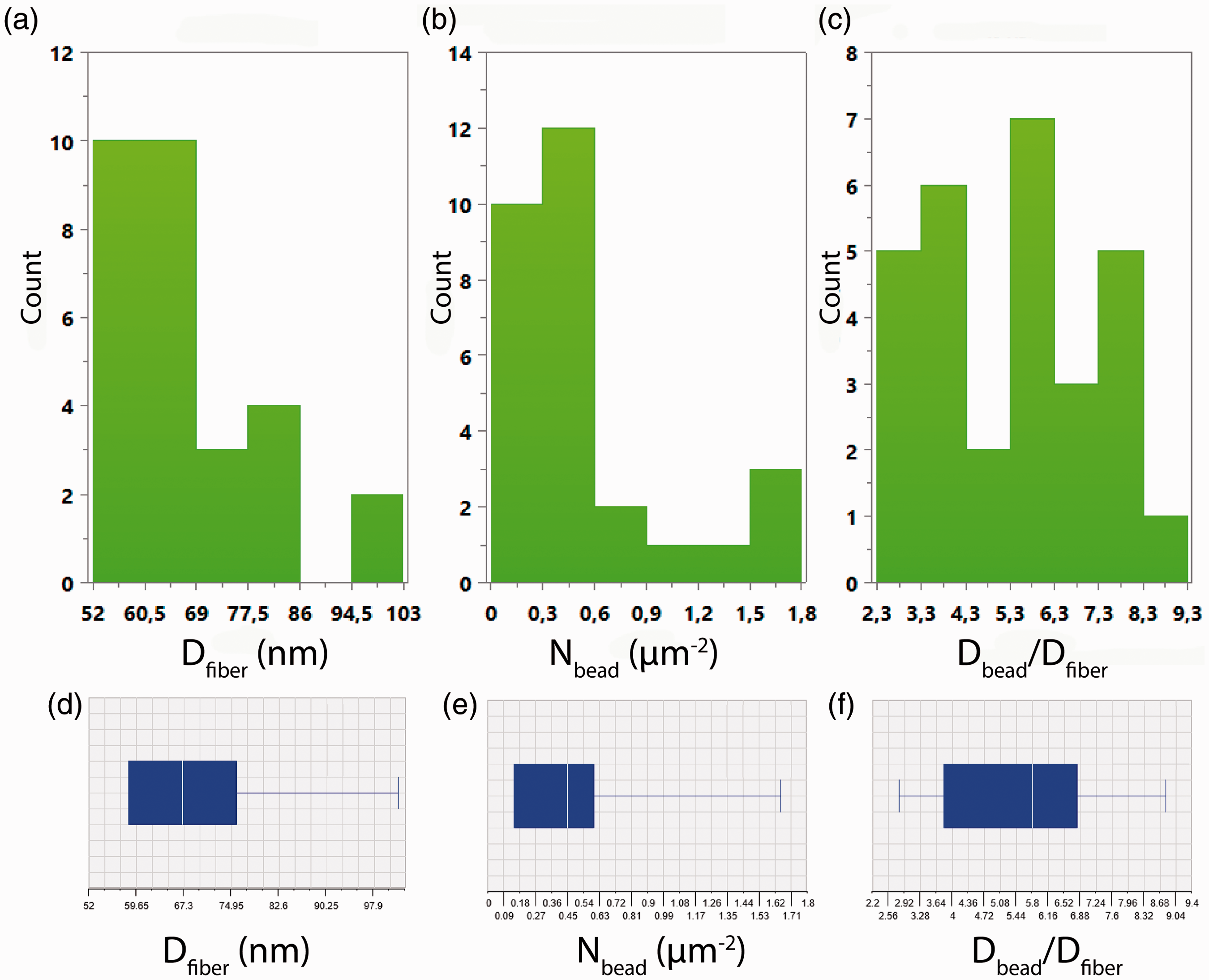

In Figure 7, the transformed responses (Y₁, Y₂, and Y₃) are shown. The transformed response data are much more symmetrically distributed than the raw response data. Hence, the distribution of the data could be regarded as normal since there is only a very small deviation from the normal distribution. Consequently, the regression analysis may reliably be performed.

Figure 7.

Histograms illustrating the transformed data distribution of the three responses: (a) transformed D_fiber (Y₁), (b) transformed N_bead (Y₂), (c) transformed D_bead/D_fiber (Y₃). The corresponding Box–Whisker plots (d,e,f) of the transformed data indicate a much more symmetrical distribution compared to the raw data.

For the transformed responses, statistical analysis results regarding the quadratic model's predictive ability (Q²), its goodness of fit (R²), its validity, and reproducibility are shown in Figure 8. The R² value denotes how well the data are fitted by the model used. Depending on the statistical problem, R² values usually should obtain values higher than 0.5, while R² values close to unity denote a perfect fit. Nevertheless, R² is quite sensitive to the degrees of freedom of system studied and it is possible to enforce R² to obtain values close to 1, arbitrarily, by including additional terms in the model.⁴⁶

Figure 8.

Transformed responses' model check based on the regression analysis (MLR) results. A bar chart of R² (green), Q² (blue), the model validity (yellow), and the reproducibility (cyan) – from left to right – for all responses is given in (a), while in (b) the aforementioned model-check values (and also $R_{adj}^{2}$ ) are tabulated.

The R² values for the transformed responses (Y₁, Y₂, and Y₃) were 0.8762, 0.9945, and 0.8764, correspondingly. These values appear to be sufficiently high that implies a good fit. Nevertheless, the quadratic equations developed in this work may include additional terms corresponding to the three-level (K, L, M) qualitative factor x₁. R² adjusted ( $R_{adj}^{2}$ ) is not quite sensitive to the degrees of freedom of the system; hence, it is not affected by comprising additional model terms. Moreover, $R_{adj}^{2}$ always obtains lower values than R². Consequently, $R_{adj}^{2}$ was examined as an additional and more reliable criterion in order to assess the goodness of the fit. The $R_{adj}^{2}$ values for the responses Y₁, Y₂, and Y₃ are 0.6849, 0.9860, and 0.6854, respectively. The $R_{adj}^{2}$ value for Y₂ should be considered to be perfect. However, the $R_{adj}^{2}$ values Y₁ and Y₃ are not quite high. The Q² parameter estimates the predictive strength of the model and at the same time it denotes the goodness of prediction. Q² is the most sensitive indicator and can take values up to unity (like R²) while a Q² value equal to 1 denotes a perfect model. However, the lower limit of Q² is minus infinity. Generally speaking, Q² values higher than 0.5 denote a good model and Q² values higher than 0.9 denote an excellent model [46]. The Q² values for the transformed responses Y₁, Y₂, and Y₃ are −0.5097, 0.9342, −0.4605 correspondingly (see Figure 8). The Q² value for the second response (Y₂) is higher than 0.9; hence it should be regarded as excellent. However, the Q² values for the other responses are negative, which indicates that there are serious model problems (i.e. the model has no predictive power) for the transformed responses Y₁ and Y₃. The third indicator “model validity” (yellow bars in Figure 8) denotes the validity of the model, and its values should be higher than 0.25 (threshold value). Significant lack of fit occurs when the model validity is below 0.25, while no lack of fit exists for values higher than 0.25. In our model, the validity is lower than the threshold value (0.25) only for the first response Y₁. Nevertheless, the acceptable model validity value (∼0.59) combined with the unacceptable Q² value, for the response Y₃, is a contradictory outcome. This contradictory result for the response Y₃ along with the not quite high values of $R_{adj}^{2}$ , coupled with the relative large deviation between R² and $R_{adj}^{2}$ and the negative values of Q² for Y₁ and Y₃ should be explained by the initial inclusion of many insignificant model terms. Additional model terms were initially included also to the models due to the three levels (K, L, M) of x₁ factor (see Table 3).

Therefore, the initially developed models should be refined by excluding insignificant model terms in order to improve the models' qualitative characteristics. The terms used in the models' equation (for each response) are shown in Table 3. Statistical analysis results (Q², R², model validity, and reproducibility) for the three responses (Y₁, Y₂, and Y₃), after model refinement are summarized in Figure 9. The model refinement was performed by deleting insignificant model terms, so as to obtain the highest possible values for Q², $R_{adj}^{2}$ , model validity, and reproducibility. A conspicuous increase in Q² (turned from negative to positive values) accompanied with a decrease in the divergence between R² and $R_{adj}^{2}$ ( $R_{adj}^{2}$ increases and at the same time R² decreases) was observed by including six model terms for the response Y₁ and only eight model terms for the response Y₃ (see Figure 9). At the same time, the model validity was increased and it was found to be higher than the threshold value (0.25) for both Y₁ and Y₃ after model refinement (see Figure 9). All the aforementioned observations indicate that good models developed after an appropriate model refinement. Moreover, it is worth noting that the model reproducibility was maintained at high levels even after model refinement.

Figure 9.

Transformed responses' model check based on the regression analysis (MLR) results after model refinement: (a) a bar-chart which illustrates R² (green), Q² (blue), the model validity (yellow), and the reproducibility (cyan) – from left to right – and (b) the aforementioned model-check values (and also $R_{adj}^{2}$ ) in table form.

Quantitative relationships between the three responses were revealed through the MLR analysis. The proposed model equations can successfully describe the experimental results obtained. Specifically, the model equations can safely predict new values within the cubic experimental region investigated and for all responses (Y₁, Y₂, and Y₃). In view of these results, the important factors for the production of nanocomposite and nanofibrous chitosan/INT-WS₂ mats could be recognized. Moreover, the optimum conditions to produce the desired electrospun morphologies may be obtained.

Important factors

The electrospinning parameters do not equally affect the three responses D_fiber, N_bead, and D_bead/D_fiber. Hence, a critical question arises: How much do the three factors affect these responses? In order to scrutinize the importance of each factor, coefficient plots were obtained (Figure 10). The coefficient plots display the regression coefficients, along with the confidence intervals (at 95% level), for all three responses (Y₁, Y₂, Y₃). Moreover, the coefficient plots can provide valuable information regarding the model interpretation: the effect of every single model term (linear, interaction, and quadratic) on the examined response could be evaluated. Hence, it is possible to detect interactions between factors by examining the effect of the interaction terms on the response of interest. The coefficient plots were produced from data that have been previously scaled and centered, due to the fact that the range of the response values is different. The data scaling rendered the regression coefficients comparable. The height of each regression coefficient bar denotes the variation in the response value, as the corresponding factor varies from 0 to 1 (coded units) and the other factors maintain their average value. Each coefficient bar may be directed either to positive or negative values, depending on the coefficient's effect on the response (i.e. increase or decrease of the response values) [46]. A regression coefficient is regarded as statistically significant (with values higher than noise), if only the confidence interval does not traverse the zero line. In that sense, a straightforward identification of the effect of each model term on the three responses (Y₁, Y₂, Y₃) can be achieved, by simply inspecting the three graphs shown in Figure 10.

Figure 10.

Coefficient plots (with their confidence intervals at 95%) for all responses: (a) Y₁, (b) Y₃, (c) Y₂.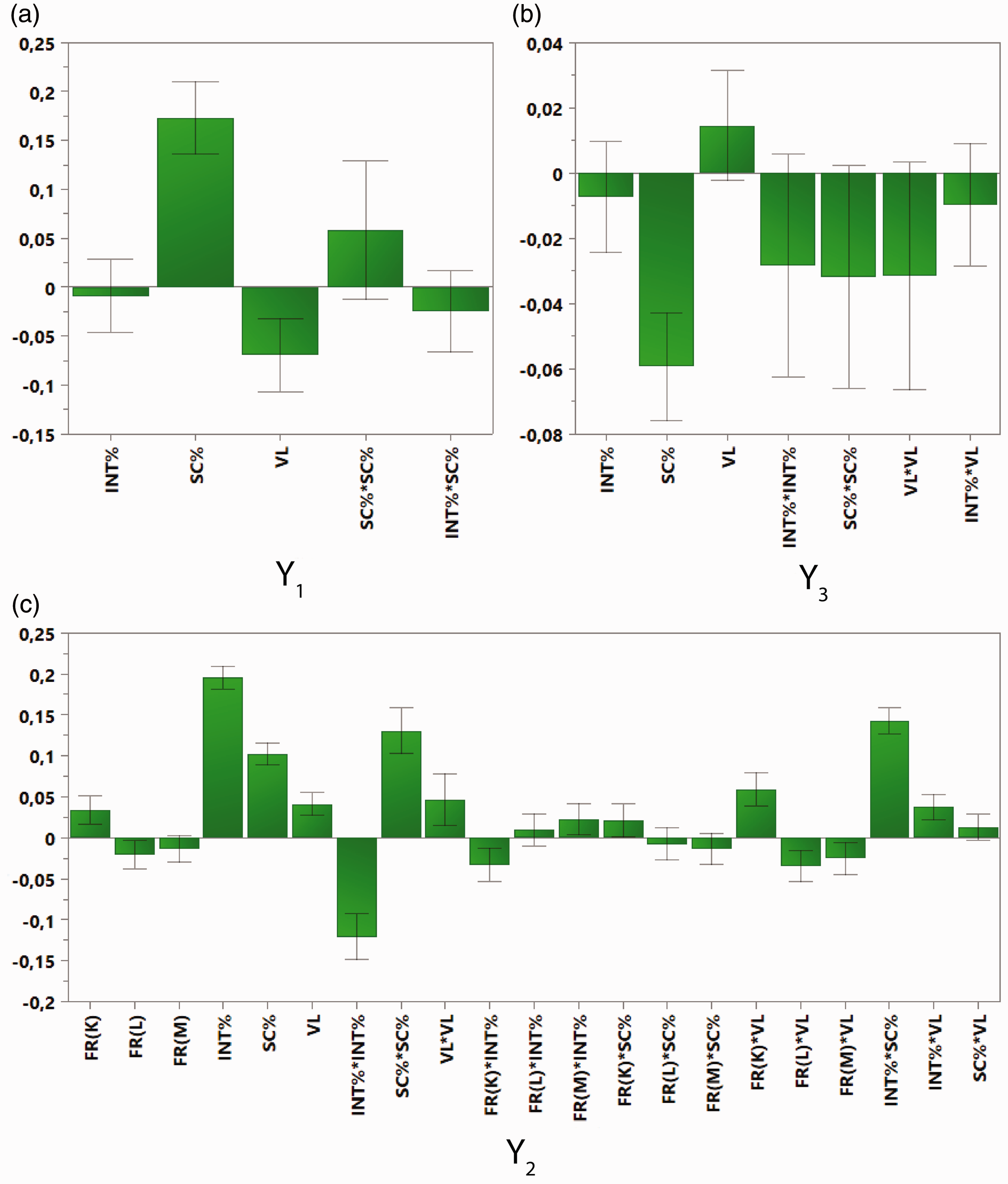

It is rather evident from Figure 10(a) that only two model terms are significant for Y₁: SC% (i.e. solution concentration) and VL (i.e. electric field strength). For the response Y₃ (Figure 10(b)) only the SC% (i.e. solution concentration) term should be considered as significant. However, for the Y₂ response 16 model terms are significant (see Figure 10(c)): FR(K) (i.e. flow rate at the K level (0.5mL/h)), FR(L), INT% (i.e. % w/v concentration of INT-WS₂), SC%, VL, INT% × INT%, SC% × SC%, VL × VL, FR(K) × INT%, FR(M) × INT%, FR(K) × SC%, FR(K) × VL, FR(L) × VL, FR(M) × VL, INT% × SC%, INT% × VL.

The polymer solution concentration (SC%) is the most significant factor for Y₁ and Y₃, having a remarkable bar height, as shown in Figure 10(a) and (b). For the Y₂ response, the polymer solution concentration is the second most significant factor. It is worth noting that the substantial influence of the polymer solution concentration does not outshine the impact of additional statistically significant terms. Furthermore, other potential trends can be found due to the fact that SC% was varied within a relatively narrow range [44]. As aforementioned in the morphology discussion (Figure 4), the polymer solution concentration (SC%) seemed to have a significant influence on the morphology of the electrospun mats. This coefficient analysis aims at the quantification of the effect of the solution concentration specifically on each geometrical characteristic (response) of the electrospun mats. Actually, when the polymer solution concentration is low, beaded and relatively thin fibers are formed regardless of the INT-WS₂ and the flow rate. When a critical concentration (3%) is reached, rather uniform nanofibers with slightly increased diameter are obtained. Beaded fibers are usually formed when the polymer concentration in the solution is low. This mainly occurs due to the low surface tension of the solution [15,49]. Electrospun mats with fewer beads are obtained, while the polymer concentration in the solution increases owing to the viscosity increase [15,49]. Moreover, various interaction terms (cross-terms), which include SC% (e.g. INT% × SC%), have a significant effect only for Y₂, while for the two other responses (Y₁ and Y₃) no cross-term appeared to have a significant effect.

The electric field strength (VL) is another important parameter of the electrospinning process. VL is the second most significant factor for Y₁ and the third most significant factor for Y₂. However, VL is not a significant factor in the case of Y₃ (Figure 10(b)). VL here appears to have a negative effect on the Y₁. The increase in the electric field strength yields narrower fiber diameters, due to the fact that the repulsive electrostatic forces increase when the electric field is strong [52]. Moreover, VL seems to have a positive impact on Y₂. It has been reported that bead formation becomes easier as the electric field becomes stronger, due to the faster charge dissipation in stronger electric fields and due to other phenomena that take place during the electrospinning process [16,53,54]. On the other hand, various cross-terms that include VL (e.g. INT% × VL) have a significant influence only for Y₂ (Figure 10(c)). This means that the electric field strength also has quite a significant effect when combined with other significant factors (e.g. INT%).

The INT-WS₂ loading (INT%) should be also be considered as an important factor. INT% is the most significant factor for the Y₂ response, since the INT% bar is much higher than the other significant factor bars with their confidence intervals not crossing zero. Nevertheless, INT% does not significantly affect Y₁ and Y₃. The addition of INT-WS₂ increases the number of beads, as aforementioned at the morphology discussion. Several cross-terms including INT% (e.g. INT% × SC%) should also be considered significant, but only for Y₂ response (Figure 10). This means that the effect of the INT-WS₂ loading is also rather significant when related to other important factors (e.g. SC%).

The fourth factor of the electrospinning process studied here, namely the flow rate (FR), should be considered a factor of minor importance, since the model terms related to FR are not quite high compared to the other three factors. However, the FR(K) and FR(L) terms are considered statistically significant, only for Y₂, but with their bars being considerably lower than the other three factors. Moreover, in the case of Y₂ response there are various cross-terms including FR(K), FR(L), or FR(M) that possess high bars (i.e. large coefficients) having confidence intervals that do not cross zero (Figure 10(c)). Two of the most statistically significant cross-terms are FR(K) × INT% and FR(K) × VL. This means that the flow rate, when combined with INT-WS₂ loading or the electric field strength, can play a crucial role on the number of beads observed on the nanofibrous electrospun mats. Nevertheless, the various cross-terms of the type FR × INT% or FR × VL change from positive to negative (e.g. FR(K) × INT% is positive, but FR(L) × INT% is negative) when increasing the flow rate from low to high values (from K to L and from K to M). Therefore, one could say that the influence of these factors included in the aforementioned cross-terms is nullified. In that sense, even though the flow rate (FR) is included in several statistically significant model terms regarding the Υ₂ response, the flow rate fails to affect considerably and systematically the formation of beads on the electrospun mats (Figure 10(c)).

Response-surface results

Response surfaces' observation provides further insights into the effects of the factors on the responses, which extend beyond phenomenological correlations. Contour plots for all responses (nontransformed) as a function of SC% and INT% at the L level of FR and at three values of VL (2, 2.3, 2.6 V/cm) are presented in Figure 11. Each column of the figure illustrates contour plots that present the variation of a certain response (D_fiber, N_bead, or D_bead/D_fiber) as a function of the two aforementioned factors (SC% and INT%). These contour plots have been calculated using the corresponding model equations for the four discrete levels of FR. However, contour plots only for the L level of FR are presented here since the flow rate does not significantly affect the resulting electrospun morphology and the contour plots for the other levels of FR (K and M) are very similar with the plots for level L.

Figure 11.

Contour plots for all responses as a function of %SC and %INT at the L level of FR and at three values of VL (2, 2.3, 2.6 V/cm). Specifically, each column of the figure illustrates contour plots that present the variation of a response (D_fiber, N_bead, or D_bead/D_fiber) as a function of the two aforementioned factors (%SC and %INT). Each row depicts contour plots for the three responses that correspond to a specific value of VL (2, 2.3, or 2.6 V/cm). The different colors in the plots denote the response value's fluctuation from low (blue) to high (red) values.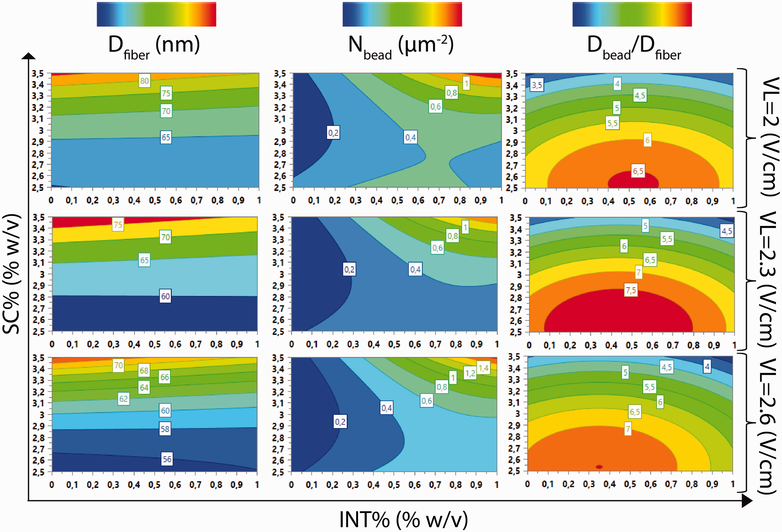

For the contour plots of the three responses for electric field strength (VL) 2 V/cm, nanofibers in the range 56–65 nm may be produced at low polymer solution concentrations. At high solution concentrations the fiber diameter (D_fiber) increases to 80 nm. Nevertheless, the INT-WS₂ loading does not affect D_fiber due to the fact that the contours are situated collaterally among each other and also situated collaterally with regard to the horizontal axis (INT%). On the other hand, the bead density (N_bead) is rather low (0.2 beads/µm) in very low INT-WS₂ loadings, while in high INT-WS₂ loadings N_bead becomes quite high (1 beads/µm). Adding to that, the combined effect of the INT-WS₂ loading and the polymer solution concentration, previously mentioned, here becomes evident: N_bead becomes quite high (1 beads/µm) if only the polymer solution concentration is also rather high (∼3.5% w/v). Moreover, at very low polymer solution concentrations (2.5% w/v) the N_bead is almost double than the N_bead for intermediate polymer solution concentrations (3% w/v) and for a certain INT-WS₂ loading. This means that if someone wants to produce rather bead-free INT-WS₂ nanocomposite chitosan nanofibers, a polymer solution concentration around 3% w/v and no or very low INT-WS₂ loadings should be chosen. This is also in accordance with our experimental findings/morphological observations. The contour plot that corresponds to the bead-to-fiber diameter (D_bead/D_fiber) has contours, which are formed ellipsoidally. Hence, D_bead/D_fiber values are increasing when the solution concentration is low and the INT-WS₂ loading obtains intermediate values (0.5 % w/v). The D_bead/D_fiber values are decreasing at higher polymer solution concentrations and the lowest possible D_bead/D_fiber values are recorded at the corners of the graph (at very low and at very high INT-WS₂ loadings).

The contour plots obtained for the rest of VL values (2.3 and 2.6 V/cm) are rather similar to the contour plots previously described (for VL = 2 V/cm). Moreover, the variation of the responses follows the trends previously described. However, the maximum and the lowest response values that can be obtained change by increasing the VL to 2.3 and 2.6 V/cm according to the trends recorded previously: the D_fiber decreases by an increase in VL, while the N_bead increases by an increase in VL. The D_bead/D_fiber values are increasing for VL = 2.3 V/cm, while in higher VL values (VL = 2.6 V/cm) D_bead/D_fiber slightly decreases. The response-surface results are in good accordance with the experimental findings.

Conclusions

A DoE study regarding the nanofibrous morphology of chitosan/INT-WS₂ electrospun mats was carried out, in the context of RSM. From the quadratic models and the subsequent analysis, we managed not only to identify but also to quantify the significance of electrospinning and material parameters (factors) on the attained nanofibrous morphology. Moreover, interactions between factors have been identified and quantified. The solution concentration (SC%), the electric field strength (VL) and the INT-WS₂ loading (INT%) were found to significantly affect the electrospun nanofibrous morphology, since they significantly affect one or more responses.

Additionally, the interpretation of the response-surface results gives directions for further research regarding the recommended electrospinning parameters for the system studied. The response-surface results revealed possible experimental pathways that one may follow in order to obtain a specified nanofibrous chitosan/INT-WS₂ morphology. Moreover, the response-surface results presented here can also be taken into consideration in order to subsequently optimize the electrospun chitosan/INT-WS₂ morphology, so as to obtain electrospun mats with optimum morphological characteristics (D_fiber, N_bead, D_bead/D_fiber) in the micro- or nanoscale. This is important due to the fact that many physical properties of the electrospun mats (e.g. hydrophobicity) depend on the morphological characteristics of the fibrous structure.

Finally, future work could be destined to the characterization and optimization of nanocomposite electrospun mats consisting of different biodegradable polymers and other types of nanofillers. This type of nanofibrous materials offers new opportunities in terms of applications.

Footnotes

Declaration of Conflicting Interests

The author(s) declare no potential conflicts of interest with respect to the research, authorship, and/or publication of this article.

Funding

The author(s) received no financial support for the research, authorship, and/or publication of this article.

Supplementary Material

Supplementary material is available for this article online.

References

Alves da Silva

Crawford

Mundy

et al.

Chitosan/polyester-based scaffolds for cartilage tissue engineering: Assessment of extracellular matrix formation. Acta Biomater 2010; 6: 1149–1157.

Nam

Park

. Biodegradable polymeric microcellular foams by modified thermally induced phase separation method. Biomaterials 1999; 20: 1783–1790.

Chen

. Techniques for fabrication and construction of three-dimensional scaffolds for tissue engineering. Int J Nanomed 2013; 8: 337–350.

Billiet

Vandenhaute

Schelfhout

et al.

A review of trends and limitations in hydrogel-rapid prototyping for tissue engineering. Biomaterials 2012; 33: 6020–6041.

Baklavaridis A, Tsivintzelis I, Zuburtikudis I, et al. Preparation of porous poly(L-lactic acid)-co-(trimethylene-carbonate) structures using supercritical CO2 as antisolvent and as foaming agent. Polym Eng Sci. 2017; 57: 1005–1015.

Baklavaridis

Zuburtikudis

Panayiotou

. Porous composite structures derived from multiphase polymer blends. Polym Eng Sci 2015; 55: 1856–1863.

Eichhorn

Hearle

JWS

Jaffe

et al.

Handbook of textile fibre structure: Fundamentals and manufactured polymer fibres, Amsterdam: Elsevier Science, 2009.

Greiner

Wendorff

. Electrospinning: A fascinating method for the preparation of ultrathin fibers. Angew Chem Int Edit 2007; 46: 5670–5703.

Reneker

Chun

. Nanometre diameter fibres of polymer, produced by electrospinning. Nanotechnology 1996; 7: 216–223.

10.

Dotti

Varesano

Montarsolo

et al.

Electrospun porous mats for high efficiency filtration. J Ind Text 2007; 37: 151–162.

11.

Shahrabi

Gharehaghaji

Latifi

. Fabrication of electrospun polyamide-66 nanofiber layer for high-performance nanofiltration in clean room applications. J Ind Text 2016; 45: 1100–1114.

12.

Gouda

Hebeish

Aljafari

. Synthesis and characterization of novel drug delivery system based on cellulose acetate electrospun nanofiber mats. J Ind Text 2014; 43: 319–329.

13.

Bosworth

Downes

. Electrospinning for tissue regeneration, Amsterdam: Elsevier Science, 2011.

14.

Wendorff

Agarwal

Greiner

. Electrospinning: Materials, processing, and applications, New York: Wiley, 2012.

15.

Subbiah

Bhat

Tock

et al.

Electrospinning of nanofibers. J Appl Polym Sci 2005; 96: 557–569.

16.

Deitzel

Kleinmeyer

Harris

et al.

The effect of processing variables on the morphology of electrospun nanofibers and textiles. Polymer 2001; 42: 261–272.

17.

Dong

Liao

Ngiam

et al.

Degradation behaviors of electrospun resorbable polyester nanofibers. Tissue Eng Pt B-Rev 2009; 15: 333–351.

18.

Jayakumar

Prabaharan

Nair

et al.

Novel chitin and chitosan nanofibers in biomedical applications. Biotechnol Adv 2010; 28: 142–150.

19.

Mitschang

Schmalz

Agarwal

et al.

Tea-bag-like polymer nanoreactors filled with gold nanoparticles. Angew Chem Int Edit 2014; 53: 4972–4975.

20.

Macagnano

Zampetti

Kny

. Electrospinning for high performance sensors, Heidelberg: Springer, 2015.

21.

Cui

Zhou

et al.

Investigation on process parameters of electrospinning system through orthogonal experimental design. J Appl Polym Sci 2007; 103: 3105–3112.

22.

Yoon

Moon

Lyoo

et al.

Superhydrophobicity of PHBV fibrous surface with bead-on-string structure. J Colloid Interf Sci 2008; 320: 91–95.

23.

Kim

. Chitin, chitosan, oligosaccharides and their derivatives: Biological activities and applications, Boca Raton, FL: CRC Press, 2010.

24.

Homayoni

Ravandi

SAH

Valizadeh

. Electrospinning of chitosan nanofibers: Processing optimization. Carbohydr Polym 2009; 77: 656–661.

25.

Geng

Kwon

Jang

. Electrospinning of chitosan dissolved in concentrated acetic acid solution. Biomaterials 2005; 26: 5427–5432.

26.

Ignatova

Manolova

Rashkov

. Electrospun antibacterial chitosan-based fibers. Macromol Biosci 2013; 13: 860–872.

27.

Cheng

Hund

Aibibu

et al.

Pure chitosan and chitsoan/chitosan lactate blended nanofibres made by single step electrospinning. Autex Res J 2013; 13: 128–133.

28.

De Vrieze

Westbroek

Van Camp

et al.

Electrospinning of chitosan nanofibrous structures: Feasibility study. J Mater Sci 2007; 42: 8029–8034.

29.

Areias

Gomez-Tejedor

Sencadas

et al.

Assessment of parameters influencing fiber characteristics of chitosan nanofiber membrane to optimize fiber mat production. Polym Eng Sci 2012; 52: 1293–1300.

30.

Ohkawa

Cha

Kim

et al.

Electrospinning of chitosan. Macromol Rapid Commun 2004; 25: 1600–1605.

31.

Cao

et al.

Enhanced chromium (VI) adsorption using nanosized chitosan fibers tailored by electrospinning. Carbohydr Polym 2014; 125: 206–213.

32.

Liu

Liao

et al.

Fabrication and durable antibacterial properties of electrospun chitosan nanofibers with silver nanoparticles. Int J Biol Macromol 2015; 79: 638–643.

33.

Min

Lee

Lim

et al.

Chitin and chitosan nanofibers: Electrospinning of chitin and deacetylation of chitin nanofibers. Polymer 2004; 45: 7137–7142.

34.

Huang

Zhang

Kotaki

et al.

A review on polymer nanofibers by electrospinning and their applications in nanocomposites. Compos Sci Technol 2003; 63: 2223–2253.

35.

Wang

Tan

Liu

et al.

Conducting MWNT/poly(vinyl acetate) composite nanofibres by electrospinning. Nanotechnology 2006; 17: 5829–5835.

36.

Numnuam

Thavarungkul

Kanatharana

. An amperometric uric acid biosensor based on chitosan-carbon nanotubes electrospun nanofiber on silver nanoparticles. Anal Bioanal Chem 2014; 406: 3763–3772.

37.

Liu

Peng

et al.

The promotion of bone regeneration by nanofibrous hydroxyapatite/chitosan scaffolds by effects on integrin-BMP/Smad signaling pathway in BMSCs. Biomaterials 2013; 34: 4404–4417.

38.

Sun

Sui

et al.

Composite mesoporous silica nanoparticle/chitosan nanofibers for bone tissue engineering. Rsc Adv 2015; 5: 17541–17549.

39.

Naseri

Algan

Jacobs

et al.

Electrospun chitosan-based nanocomposite mats reinforced with chitin nanocrystals for wound dressing. Carbohydr Polym 2014; 109: 7–15.

40.

Rothschild

Sloan

Tenne

. Growth of WS2 nanotubes phases. J Am Chem Soc 2000; 122: 5169–5179.

41.

Goldman

Zak

Tenne

et al.

Biocompatibility of tungsten disulfide inorganic nanotubes and fullerene-like nanoparticles with salivary gland cells. Tissue Eng, Part A 2015; 21: 1013–1023.

42.

Kaplan-Ashiri

Cohen

Gartsman

et al.

Mechanical behavior of individual WS2 nanotubes. J Mater Res 2004; 19: 454–459.

43.

Ristolainen

Heikkilä

Harlin

et al.

Poly(vinyl alcohol) and polyamide-66 nanocomposites prepared by electrospinning. Macromol Mater Eng 2006; 291: 114–122.

44.

Tsimpliaraki

Svinterikos

Zuburtikudis

et al.

Nanofibrous structure of nonwoven mats of electrospun biodegradable polymer nanocomposites - A design of experiments (DoE) study. Ind Eng Chem Res 2009; 48: 4365–4374.

45.

Montgomery

. Design and analysis of experiments, 8th ed. New York: Wiley, 2012.

46.

Eriksson

Johansson

Kettaneh-Wold

et al.

Design of experiments principles and applications, Umea: Umetrics, 2000.

47.

Costolo

Lennhoff

Pawle

et al.

A nonlinear system model for electrospinning sub-100 nm polyacrylonitrile fibres. Nanotechnology 2007; 19: 035707

48.

Doube

Klosowski

Arganda-Carreras

et al.

BoneJ: Free and extensible bone image analysis in ImageJ. Bone 2010; 47: 1076–1079.

49.

Fong

Chun

Reneker

. Beaded nanofibers formed during electrospinning. Polymer 1999; 40: 4585–4592.

50.

Zhang

Yuan

et al.

Study on morphology of electrospun poly(vinyl alcohol) mats. Eur Polym J 2005; 41: 423–432.

51.

Ramakrishna

. An introduction to electrospinning and nanofibers, Singapore: World Scientific, 2005.

52.

Yuan

Zhang

Dong

et al.

Morphology of ultrafine polysulfone fibers prepared by electrospinning. Polym Int 2004; 53: 1704–1710.

53.

Demir

Yilgor

et al.

Electrospinning of polyurethane fibers. Polymer 2002; 43: 3303–3309.

54.

Buchko

Chen

Shen

et al.

Processing and microstructural characterization of porous biocompatible protein polymer thin films. Polymer 1999; 40: 7397–7407.

Supplementary Material

Please find the following supplemental material available below.

For Open Access articles published under a Creative Commons License, all supplemental material carries the same license as the article it is associated with.

For non-Open Access articles published, all supplemental material carries a non-exclusive license, and permission requests for re-use of supplemental material or any part of supplemental material shall be sent directly to the copyright owner as specified in the copyright notice associated with the article.

0.00 MB

0.40 MB

Exp. No.	Exp. name	Run order	x₁ = FR (K, L, M)	x₂ = INT%	x₃ = SC%	x₄ = VL
1	N1	13	L	0	2.5	2
2	N2	28	M	0	2.5	2
3	N3	9	K	0.5	2.5	2
4	N4	7	M	1	2.5	2
5	N5	21	K	0	3	2
6	N6	6	L	1	3	2
7	N7	4	L	0	3.5	2
8	N8	10	M	0	3.5	2
9	N9	11	L	0.5	3.5	2
10	N10	26	K	1	3.5	2
11	N11	14	M	1	3.5	2
12	N12	27	K	1	2.5	2.3
13	N13	2	L	1	2.5	2.3
14	N14	15	M	0.5	3	2.3
15	N15	18	K	0	3.5	2.3
16	N16	24	M	1	3.5	2.3
17	N17	1	K	0	2.5	2.6
18	N18	22	M	0	2.5	2.6
19	N19	16	L	0.5	2.5	2.6
20	N20	29	M	1	2.5	2.6
21	N21	8	L	0	3	2.6
22	N22	12	K	1	3	2.6
23	N23	5	L	0	3.5	2.6
24	N24	19	M	0	3.5	2.6
25	N25	23	K	0.5	3.5	2.6
26	N26	25	L	1	3.5	2.6
27	N27	3	M	0.5	3	2.3
28	N28	17	M	0.5	3	2.3
29	N29	20	M	0.5	3	2.3

Exp. No.	Exp. name	Run order	x₁ = FR (K, L, M)	x₂ = INT%	x₃ = SC%	x₄ = VL
1	N1	13	L	0	2.5	2
2	N2	28	M	0	2.5	2
3	N3	9	K	0.5	2.5	2
4	N4	7	M	1	2.5	2
5	N5	21	K	0	3	2
6	N6	6	L	1	3	2
7	N7	4	L	0	3.5	2
8	N8	10	M	0	3.5	2
9	N9	11	L	0.5	3.5	2
10	N10	26	K	1	3.5	2
11	N11	14	M	1	3.5	2
12	N12	27	K	1	2.5	2.3
13	N13	2	L	1	2.5	2.3
14	N14	15	M	0.5	3	2.3
15	N15	18	K	0	3.5	2.3
16	N16	24	M	1	3.5	2.3
17	N17	1	K	0	2.5	2.6
18	N18	22	M	0	2.5	2.6
19	N19	16	L	0.5	2.5	2.6
20	N20	29	M	1	2.5	2.6
21	N21	8	L	0	3	2.6
22	N22	12	K	1	3	2.6
23	N23	5	L	0	3.5	2.6
24	N24	19	M	0	3.5	2.6
25	N25	23	K	0.5	3.5	2.6
26	N26	25	L	1	3.5	2.6
27	N27	3	M	0.5	3	2.3
28	N28	17	M	0.5	3	2.3
29	N29	20	M	0.5	3	2.3

Nanofibrous morphology of electrospun chitosan nanocomposites reinforced with WS2 nanotubes: A design-of-experiments study

Abstract

Keywords

Introduction

Experimental section

Materials

Preparation of the nanocomposite electrospun mats

Experimental design and responses

Morphological characterization and statistical analysis

Results and discussion

Morphology

Raw response data assessment and regression analysis

Important factors

Response-surface results

Conclusions

Footnotes

Declaration of Conflicting Interests

Funding

Supplementary Material

References

Supplementary Material

Exp. No.	Exp. name	Run order	x₁ = FR (K, L, M)	x₂ = INT%	x₃ = SC%	x₄ = VL
1	N1	13	L	0	2.5	2
2	N2	28	M	0	2.5	2
3	N3	9	K	0.5	2.5	2
4	N4	7	M	1	2.5	2
5	N5	21	K	0	3	2
6	N6	6	L	1	3	2
7	N7	4	L	0	3.5	2
8	N8	10	M	0	3.5	2
9	N9	11	L	0.5	3.5	2
10	N10	26	K	1	3.5	2
11	N11	14	M	1	3.5	2
12	N12	27	K	1	2.5	2.3
13	N13	2	L	1	2.5	2.3
14	N14	15	M	0.5	3	2.3
15	N15	18	K	0	3.5	2.3
16	N16	24	M	1	3.5	2.3
17	N17	1	K	0	2.5	2.6
18	N18	22	M	0	2.5	2.6
19	N19	16	L	0.5	2.5	2.6
20	N20	29	M	1	2.5	2.6
21	N21	8	L	0	3	2.6
22	N22	12	K	1	3	2.6
23	N23	5	L	0	3.5	2.6
24	N24	19	M	0	3.5	2.6
25	N25	23	K	0.5	3.5	2.6
26	N26	25	L	1	3.5	2.6
27	N27	3	M	0.5	3	2.3
28	N28	17	M	0.5	3	2.3
29	N29	20	M	0.5	3	2.3