
Abstract
This paper presents a demonstrative application of a forward model-driven approach to structural health monitoring (SHM), incorporating hierarchical validation methods. A key tenet of the approach is that an SHM system can be constructed that is capable of diagnosing damage at the full system level, without full system damage-state data having been used in its development; achieving this would be highly impactful as the system-level damage state data is generally not feasible to acquire (previous SHM methods such as data-driven SHM have been hindered by their dependence on these data). This is achieved by carrying out validation activities on the damage model at the subassembly level of the structure. The particular focus of the present paper is on damage detection and assessment, although the approach offers a natural basis for extension to other damage identification activities such as damage location and prognosis. The present study focuses on two of the key elements of the model-driven approach: validation of the predictive substructure models and their application in the assembled model. The ideas discussed are demonstrated in a case study based on a laboratory-scale truss bridge structure.
Keywords
Introduction
Approaches to structural health monitoring (SHM) can be broadly separated into two categories: data-driven and model-driven methods. Data-driven methods rely on structural data to infer the normal operating condition of a structure using some machine learning process, whereas model-driven methods use physics-based models to infer the health state of a structure by comparing the predictions of the models to structural data.
Data-driven methods for SHM have had significant success in recent decades as the field of machine learning has advanced significantly; simultaneous advancements in computational capabilities and sensor placement techniques have also been key. However, since data-driven methods are dependent on labelled training data for the machine learning processes, many SHM applications present significant difficulties. The foremost among these is the ability to acquire data from structures in their damaged states. 1 Without these data, data-driven SHM is limited to novelty detection methods, which, while applicable to damage detection problems, are not suitable to more refined problems such as damage localisation or assessment. This therefore motivates the use of predictive models to simulate the data required for training statistical models.
Model-driven methods can be further divided into approaches that use a parameter updating scheme to infer the presence of damage, and approaches that use model predictions to simulate training data for statistical damage detectors, as described above. Due to their basis on knowledge of physics, model-driven SHM methods are well-suited to all levels of Rytter’s hierarchy (which describes the tasks commonly associated with a complete SHM strategy; damage detection, localisation, assessment and prognosis). 2 By contrast, advanced data-driven methods have been applied to the first three levels of the hierarchy, 3 but due to the lack of physical insight involved in their development, it is not possible for them to provide any information regarding damage prognosis or remaining life assessment.
Inverse model-driven structural health monitoring (IMD-SHM) has been applied successfully in industry,4,5 but suffers from two key issues. The first issue is that the parameter updating problem used to match the model predictions to structural data, and thus infer damage, can be highly unstable. Rigorous constraint of the problem is required in the development stage of the strategy in order to avoid issues such as lack of solution uniqueness. The other main issue, which affects the application of all models, is the paradigm that all models are ‘wrong’. 6 The inherent inaccuracy of predictive models is usually mitigated by verification and validation (V&V) to ensure that models are sufficiently accurate and robust for a given application, with any associated uncertainties in the model quantified. However, in the context of SHM, this can become difficult as comparison to structural damage-state data is required in order to validate predictive damage models; this, as discussed previously, can be unfeasible to acquire.
The use of models in a forward, predictive, capacity – here termed forward model-driven structural health monitoring (FMD-SHM) – offers potential improvements on both classic IMD-SHM and data-driven methods. By avoiding the parameter updating problem used in IMD-SHM, many computational issues in executing the strategy are avoided. In addition, using the numerical model to generate training data for a statistical damage classifier avoids the need to acquire large training datasets experimentally. The key drawbacks of FMD-SHM are that the design and development of predictive models for SHM are still difficult undertakings, and the models still require validation in order to be used with confidence. This usually means that some level of damage-state data is required from the target structure in order to ensure the accuracy of the model’s damage-state predictions.
One particular motivation for the development of FMD-SHM is that it offers significant potential for development of the strategy at the design and development stage. This has been identified as a significant step required to make SHM systems more applicable to industry. 7 One way in which the cost of implementation of an FMD-SHM strategy can be reduced is by performing validation at the subassembly level. This would then alleviate the requirement for assembly-level damage state data, provided that the uncertainty quantified at the subassembly level can be robustly propagated upward through the model hierarchy. This idea of hierarchical V&V is key to the ideas discussed in this paper.
Hierarchical V&V is popular in a range of disciplines,8,9 but has not yet been considered as a means to reduce the cost of SHM system development. In addition, despite a number of promising studies,10–12 the use of FMD-SHM as a strategy in itself has received limited attention in the field. This paper demonstrates these concepts and the associated ideas through a case study that focuses on a laboratory-scale truss bridge; to the authors’ best knowledge, this will be the first published paper to explicitly demonstrate the applicability and performance of a hierarchical V&V strategy to a realistic SHM case study. The aim is to show that there is significant potential to reduce the dependence of SHM systems on highly expensive datasets without significant loss of classification accuracy, in the context of damage detection and assessment, compared to data-driven SHM methods.
A high-level framework for the implementation of an FMD-SHM strategy using hierarchical V&V methods is given in Figure 1. This provides the basis for the implementation of the hierarchically-validated SHM strategies and will be explored in this paper. The case study in this paper aims to demonstrate the feasibility of the forward model-driven approach, while highlighting the potential cost reductions that are available by implementing a hierarchical V&V strategy. This will be done by following the framework discussed in this paper to train a damage detector and regression model for an experimental bridge structure, using training data generated by a physics-based model which has been validated without the use of assembly-level damage data. The exact workflow followed in this case study may require development in other applications, particularly where the SHM strategy could be extended other tasks, but the underlying philosophies should be consistent, and it is hoped that the paper will clearly motivate further research into the potential of these ideas.
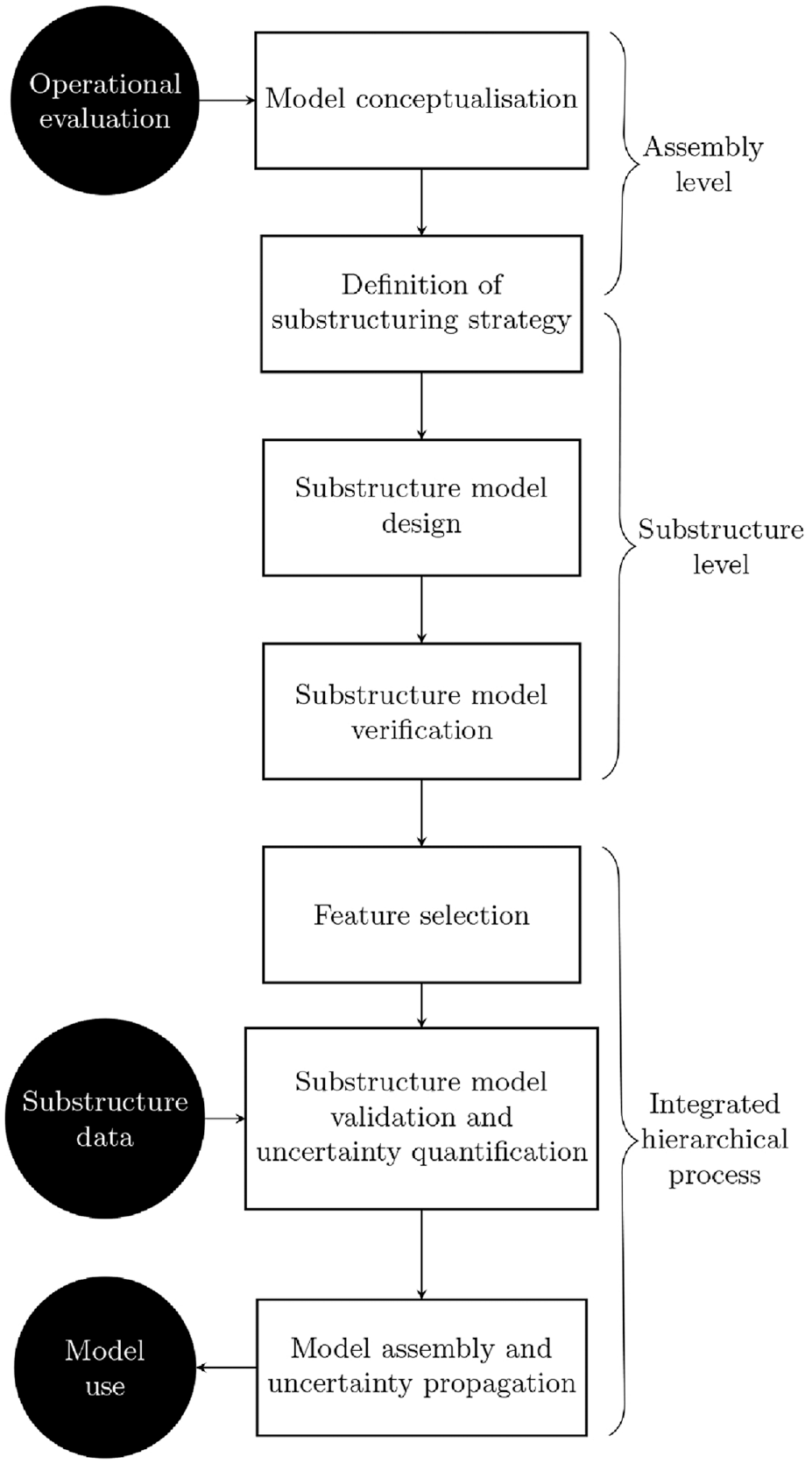
Proposed framework for hierarchical verification and validation.
The paper proceeds by presenting the methodologies for FMD-SHM, hierarchical V&V, and dynamic substructuring. This is then followed by a case study covering V&V activities, damage detection and damage assessment using the hierarchical V&V and FMD-SHM methodologies. The case study is then discussed and suggestions for future research are presented. The paper builds on the work presented in Wilson et al.13–15; it extends their findings by applying the models in an SHM context, and comparing the results against traditional data-driven methods.
Methodology
The methodology utilised in this paper for is based on the techniques of FMD-SHM and hierarchical V&V; the theoretical backgrounds for these techniques are presented as follows. Hierarchical V&V has been shown to be implementable using dynamic substructuring techniques 13 ; dynamic substructuring is therefore also presented as part of the methodology.
Forward model-driven structural health monitoring
This section aims to outline a general strategy for determining the health state of a system based on observed features generated as part of an FMD-SHM strategy. A simple strategy for damage detection would proceed as follows:
1. Use the model to make system-level predictions across health states of interest with any associated uncertainty.
2. Define an acceptable damage threshold for each class of damage (e.g. maximum permissible crack length).
3. Label the predicted data as belonging to either the undamaged class or damaged class.
4. Train a classifier using predicted training data and apply it to predict the global health state of the structure when presented with new test data. Options include:
• Building a non-probabilistic classifier: Train a classifier using labelled training data; when test data are presented, report the predicted class label.
• Using a probabilistic approach: Learn the distribution of the training data; when test data are presented, report the probability of class membership.
While the above is conceptually simple, challenges nonetheless arise and a number of decisions must be taken by the system designer. Setting of a threshold (which determines the decision boundary for the classifier) on acceptable damage is key among these. The compromise here is between maximising the true positive rate (TPR) and minimising the false positive rate (FPR). In industry, significant risk analysis and safety evaluation must be taken into account at this stage.
In principle, the damage detection strategy could be extended to both damage localisation, classification and identification of (discrete) damage extent by expanding the set of health states that are considered. Alternatively, regression methods may be used to arrive at a continuous valued prediction where required. Both damage detection and damage assessment – using regression methods – are demonstrated in this paper.
Hierarchical V&V
In order to ascertain the accuracy and reliability of representative models of reality, their predictions must be ratified against actual observations from reality. This forms a significant portion of the V&V process and is critical in establishing model-driven systems that require any level of confidence in their predictions or outcomes. The term verification refers to the efforts to ensure that the model is accurate in its attempts to estimate a given solution, and therefore considers factors such as discretisation errors and errors of numerical model design. 16 Validation refers to the efforts to ensure that the model is an accurate estimation of reality, and the solutions it attempts to derive are representative of real-life observations; it therefore considers model discrepancies or biases and random errors. 16
The concept of uncertainty can be separated into two contributors to overall lack of knowledge: epistemic and aleatoric uncertainty. Aleatoric uncertainty, also known as irreducible uncertainty, pertains to unavoidable uncertainties inherent to a problem that cannot be reduced with additional knowledge. Aleatoric uncertainty is generally unbiased and random and can therefore be captured and estimated in the V&V process. Epistemic uncertainty, also known as systematic uncertainty, pertains to uncertainties due to actual lack of knowledge, for example in the case of model simplification or assumptions leading to certain physical processes being neglected from the problem. 17
Error refers to the difference between an estimation and the true solution and is unavoidable when any level of uncertainty is present. Random errors are generally considered the more benign of the two types, and manifest in a scattering of predictions around a mean value that can be described by some statistical model. Systematic errors, which are also referred to as model discrepancy or model bias, refer to a repeated offset between the prediction and the true value; these can be described by a particular function based on a set of input parameters.
Physics-based models can be used for SHM purposes in a variety of ways. IMD-SHM refers to model updating methods whereby a models input parameters are updated in order to align its predictions with live structural data; this allows for damage to be inferred from the state of the model inputs. 1 Models can also be used in a forward sense, where their predictions are used to provide training data for statistical machine learning models for damage inference. 1 In order to validate a model for each of these purposes, damage-state data must be acquired for comparison with damage-state predictions. This leads to a series of difficulties when conducting V&V in a SHM context, summarised below:
1. Target structures may be of prohibitively high value to carry out invasive or damaging data acquisition processes.
2. If the target structure is unique, usage requirements and other factors may restrict the data acquisition process, limiting the types of testing that can be performed.
3. The target structure may be difficult to scale or transport in such a way as to allow well-designed, controllable laboratory tests.
4. The design or operating environment of the target structure may make sensor placement difficult.
5. The operating condition of the structure may be difficult to replicate in order to acquire representative validation data.
Notwithstanding some successes,18–20 model-driven SHM has been significantly handicapped in its applicability in industry due to the issues outlined above. This motivates further research into the advancement of V&V techniques to mitigate the current difficulties.
Hierarchical V&V allows confidence to be ascribed to the predictions of an assembly-level model. This is achieved by using subassembly data to validate a series of submodels separately and then constructing an assembly-level model from the validated submodels. The uncertainty can be quantified at the assembly level by propagating the uncertainty from the subassembly levels upwards, thereby establishing quantifiable confidence in the predictions of the assembly-level model. Hierarchical V&V offers the potential to improve the feasibility of model-driven SHM in the long term for the following reasons:
1. The method avoids the need to acquire damage-state data from assemblies that represent high capital investment.
2. Design of experiments can take advantage of repeated subassemblies or components, particularly in the case of modularity or symmetry of components, to reduce the extent of testing required.
3. Ease of data acquisition can be improved as smaller-scale and simpler structures are required for testing.
4. The testing of simpler structures could increase ease of sensor placement.
An extension of this logic could be applied to target structures that form part of a population, for example in the case of wind farms or airline fleets. Individual structures in these populations may not be identical in truth, but they may share nominally identical components or subassemblies. The ability to validate substructures in this context would offer strong value gains in the SHM of populations.
Outside of the field of V&V, hierarchical model use has its own set of potential benefits. A key advantage of submodelling is the ability it grants to focus model resolution, and therefore computational effort, in facets of the model assembly that are integral to its behaviour. 21 This therefore allows for more parsimonious model design. Another benefit is that submodelling naturally allows for a division of labour; this would allow modelling departments within companies to effectively manage large projects and workloads collaboratively.
Hierarchical V&V (and hierarchical model design in general) does present certain difficulties. The foremost issue with using hierarchical V&V in SHM is the question of how to quantify the uncertainty in the submodels, and then propagate this uncertainty through the assembly process. Handling of uncertainties in a complex model can often lead to extremely computationally intensive activities, for example in the use of random sampling methods to propagate input uncertainties through to model predictions. In addition, while aleatoric uncertainty is a relatively well-understood discipline, the quantification and handling of epistemic uncertainty is an open research question, particularly where it may be introduced in the assembly process. Consideration into how this would affect the ability to assign confidence to an assembly-level model based on a set of validated submodels must be taken into account.
The particular issue of epistemic uncertainty associated with substructure assembly is closely linked to the question of how to model the interfaces between the substructures. Joint behaviour can greatly affect the dynamic behaviour of a structure, and therefore presents a potential pitfall if not properly accounted for during the assembly process. It could also be very difficult to model joint behaviours from the assembly as boundary conditions of the submodels. The submodels should be validated over a range of operating conditions that would reflect the conditions that they are placed under in the full assembly. This could potentially be difficult to capture in the design of experiments for acquiring validation data. On the other hand, the use of submodels does offer the potential for joints to be considered in special detail, where bespoke interaction models could be designed to reflect complex physical behaviours. Given the large area of research that concerns the modelling of various types of joints, specialist knowledge could be readily incorporated into the process here.
Finally, a potential drawback of hierarchical V&V is the effect of local versus non-local, or global, behaviours. In designing and validating the submodels for SHM, modellers must make sure to focus on model behaviours that would allow for global damage detection in the assembly and are not sensitive to local effects only. In addition, it is important to validate the submodels over a range of damage conditions; therefore, the features used for this process must be damage-sensitive at the submodel (local) level. A full discussion on the handling of features in a hierarchically validated system for FMD-SHM can be found in Wilson et al. 14
Dynamic substructuring
Dynamic substructuring is the term for a group of methods designed for the assembly or disassembly of predictive models of dynamic systems and, as such, is integral to this paper. 21 In terms of nomenclature, the following definitions for dynamic substructuring are presented in this paper:
In assembly of a set of substructures, conditions need to be defined which describe the interface behaviour at the joints. The two key defining conditions are degree-of-freedom (DoF) compatibility, and interface force equilibrium. The simplest compatibility constraint is to set the responses to be equal at the interface; however, this can be altered in order to improve accuracy in modelling of joints.
The compatibility condition is enforced by defining a matrix, B (the compatibility matrix). B is a signed Boolean matrix; in the case of rigid connections, it is defined such that its product with x (the response vector of the substructures) is the zero vector (Equation (1)). The dimensions of B are the number of interface connections in assembly by the number of unassembled DoFs.
In addition to DoF compatibility, the interface forces must satisfy the constraint of equilibrium in assembly. This constraint is enforced by the matrix L (the localisation matrix), which is defined such that the product of its transpose with g, the vector of interface forces, is equal to zero (Equation (1)), in the case of rigid connections at the interfaces. It should be noted that internal forces are present in all masses, but do not generally contribute to dynamic behaviour (or are neglected from most models). However, the forces at the interface of an assembly must be combined to describe a new set of internal forces within the new lumped mass. The localisation matrix is an unsigned Boolean matrix whose dimensions are the number of unassembled DoFs by the number of DoFs in the assembly. L will also map the global vector of assembled DoFs,
For a substructuring problem under the assumption of rigid joint connections, the assembly can be represented using the three-field formulation (see Equation (1)). The mass

The substructuring problem can be approached via several methods, depending on the information available to the modeller and the intended application of the model. There are two overarching mathematical processes for the assembly of substructures: primal and dual assembly. These are equivalent to each other mathematically, but each lends itself to different techniques and situations.
21
Starting with the three-field formulation, to apply primal assembly, Equation (2) is substituted into Equation (1) to eliminate redundant response entries from the equation of motion. Following this, the equation is premultiplied by

Direct physical assembly of substructures can be carried out simply using the primal assembly method. To derive the assembled and updated parameter matrices (
This method has been applied successfully in previous exploratory investigations into the hierarchical V&V process.13,15 Other dynamic substructuring methods available include frequency-based substructuring (via dual assembly) and model reduction methods such as Craig–Bampton; the reader is referred to Allen et al. 21 for further information on these.
In any dynamic substructuring procedure, the assembly is carried out by applying physical constraints to the substructures that define the joints in some way. Therefore, it is critical that these constraints and their impact on the assembly model are fully understood. Assumptions that are made to simplify the dynamic substructuring assembly process, such as the assumption of rigid connections (which has been used in the above derivations), must be stated, and attempts to quantify the discrepancy they introduce are highly recommended.
Case study
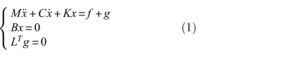
The aims of this case study were to demonstrate that hierarchical V&V could be applied to SHM problems and achieve similar performance to more established SHM methods such as data-driven SHM. Hierarchical V&V could be carried out by validating submodels of the larger assembly and assembling these via dynamic substructuring. The assembled models could then be used to generate training data according to the FMD-SHM paradigm. The case study made use of a laboratory-scale truss bridge structure at the University of Sheffield’s Laboratory for Verification & Validation, shown in Figure 2. The truss bridge is a popular design in civil engineering, comprising a solid deck with a rigid upper assembly of struts that bear the load on the deck. The structure was ideal for this study as it could be easily broken down into a series of subassemblies and components: the deck, the struts and the upper frame holding the struts together. A similar style of bridge in Leuven was studied in an SHM context in Maes and Lombaert. 22
The laboratory-scale truss bridge used for this case study.
The submodels of the bridge for this study was constructed from finite elements in ANSYS Mechanical using APDL. The strut components were cut from thin aluminium plate and were modelled as simple beam structures; collectively, the struts could be considered as a substructure of the bridge. The upper frame consisted of a rectangular beam structure with an additional cross member at its midpoint; the beam components of this subassembly were lengths of aluminium Rexroth. The deck subassembly consisted of a thin aluminium plate bordered by a rectangular Rexroth frame. These subassemblies represented the key substructures of the assembly, and were therefore selected for development as separate submodels.
The assembly model was constructed from the submodels using the primal assembly method of dynamic substructuring in the physical domain. The joint components, which consisted of a range of bolts, washers, nuts and brackets were neglected from the model. The joints between substructures were assumed to be rigid and coincident with the nodes on the submodels nearest to the actual joint location on the real structure. These simplifications drastically reduced the complexity of the assembly process, meaning that the compatibility matrix could be derived analytically when a list of the joint nodes on each submodel was provided; however, it must be acknowledged here that some amount of model discrepancy would be added to the assembly model by simplifying the joints in this manner.
The model was designed to provide predictions of the modal behaviour of the bridge based on a set of inputs and parameters. The inputs to the model describe the damage condition and entailed the damaged strut, the location of the crack on the strut and the depth of the crack. The parameters of the model entailed the material properties and the crack model parameters. Uncertainty could be quantified in the model by fitting distributions to each parameter through V&V.
In order to evaluate the natural frequencies and modes shapes of the substructures, an eigenvalue solution was obtained using the mass and stiffness matrices of the submodels. Due to the nature of the deck as a thin plate, the aspect ratio of the elements used in this substructure were very high, which led to poor conditioning of the mass matrix of the deck and assembly. This then meant that the inversion of the mass matrix could cause potential inaccuracies, a process which was required in computing the eigenvalue solution. Cholesky decomposition was used in order to carry out the Krylov–Schur algorithm for computing a subset of eigenvalues pertaining to the low modes of the model. This process was verified by comparing the product of the decomposed matrices to the original matrix, which was found to have very low error.
The beam crack models investigated in this study were based on Friswell and Penny 23 ; this paper reviews four open crack modelling methods and compares them against experimental data – the vast majority of damage models for beams can be categorised as one of these overall techniques. The methods can be categorised as follows:
Element stiffness reduction methods
– This method reduces the stiffness of the element where the crack is located on the beam.
– The two key inputs are the location of the element and the magnitude of the stiffness reduction.
– The stiffness reduction can be related to the crack depth by reducing the depth of the element at the crack location by the crack depth – this has the benefit of adding physical interpretability to the model inputs.
– An additional parameter is crack width (the length of the element at the crack location). This gives greater control of the model but means that the beam requires remeshing for different parameters.
Discrete spring methods
– This method replaces the continuum beam model with a spring at the crack location of variable stiffness.
– The inputs to the model are the spring stiffness, which is based on the depth of the true crack, and the crack location.
– The physical interpretability of this model is low, and the damage magnitude is only controllable through the spring stiffness, which does not allow for independent control of crack depth and width.
Element removal methods
– This method is based on beam models with 3D meshes.
– Elements can be removed entirely from these meshes to best match the removal of material observed in the real crack.
– This method is the most physically representative, and can be used to very precisely model the geometry of a crack, but has relative high computational cost due to its dependence on fine meshes.
Stiffness distribution methods
– This method uses a law to describe the distribution of the stiffness across the whole length of a cracked beam.
– Many distributions can be used; the Christides and Barr 24 and Sinha 25 distributions were tested in Friswell and Penny. 23 A Gaussian distribution was used in Bruns et al. 26
– The accuracy of the method is entirely dependent on the distribution law selected; significant disparities were observed between the accuracy of the Sinha distribution and the Christides and Barr distribution in Friswell and Penny. 23
Three candidate models were identified for this case study, described in the following sections. Given that the strut submodel was constructed as a solid beam of 2D line elements, element removal methods were not applicable in this case. Discrete spring methods were also not investigated for this case study.
Model 1
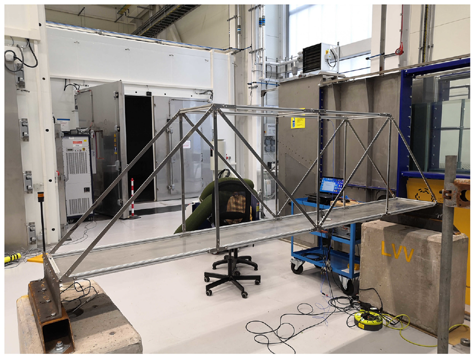
Model 1 was essentially an element stiffness reduction damage model. The inputs to the model were crack depth and location on the strut. The element at the crack location was then reduced in stiffness by reducing its cross-sectional depth by the depth of the crack, with the centroid offset from the undamaged elements as shown in Figure 3. The key tuneable parameter of the model was crack width
Graphical representation of damage model 1 with inputs and parameters marked (x, d and w represent distance, depth and width respectively).
Model 2
Model 2 was an extension of model 1 with an additional tuneable parameter that controlled the Young’s modulus of the element at the damage location,
Model 3
Model 3 was a stiffness distribution damage model which used a Gaussian distribution to describe the Young’s modulus at each node of the model, as was demonstrated in Bruns et al.
26
The inputs were
Submodel verification
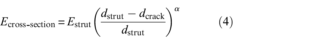
Verification was carried out in this study by comparison of numerical results to analytical solutions where possible, and by grid convergence analysis using the Richardson Extrapolation 27 and the grid convergence index (GCI). 16 The models investigated included nominal strut and plate models, used to verify the accuracy of the ANSYS BEAM188 and SHELL181 elements used to construct these elements, respectively. These basic models were verified against analytical solutions calculated using the Blevins’ formulae for natural frequencies. 28 The bridge substructures (struts, upper Rexroth, deck) were then all subjected to grid convergence analyses.
BEAM188, which was used for the struts and Rexroth, is a two-node element in the ANSYS library designed for analysis of beam structures. Each of the nodes has six DoFs as standard (plus an optional warping DoF) and the element can be evaluated by linear, quadratic or cubic laws based on Timoshenko beam theory. 29 BEAM188 is a 1D line element with cross-section data specified separately to make it 3D, allowing it to be tailored to both the thin strut and the more complex Rexroth geometries.
To verify the accuracy of the beam elements used for the strut and Rexroth sections of the model, a nominal case was set up to compare the solutions of a modal analysis to a set of equivalent analytical solutions. 28 The assumptions made for this solution are that the beam is of uniform cross-section with dimensions much less than the length of beam, the material is linear, homogeneous and isotropic, the beams can only deflect normal to the undeformed axes, no axial loads are applied, and the rotation and translational motions of the beam are not coupled. The rotational modes were calculated separately, under the same assumptions as the translational modes but for pure rotational motion uncoupled from any translational motion.
The case modelled a cantilever beam of length 1000 mm, with height 20 mm and thickness 4 mm. The Young’s modulus was set to
The error between the analytical solution and the model predictions of the first 10 modes for the BEAM188 elements.
SHELL181 is designed for analysis of thin shell structures, and was applied to the deck in this analysis. Each element has four nodes, each of which has six DoFs as standard. SHELL181 is a 2D area element, where the thickness is defined separately (it is suitable for laminate as well as homogeneous shells). The number of integration points within each element is optional, the default being three.
Similarly to with the beam elements, a nominal case was set up to compare the shell element formulations to a set of analytical solutions. The shell elements were used to construct the plate in the deck substructure, which was bordered in the model by a Rexroth beam structure. As for beams, the rectangular plate is a suitably simplistic member that its natural frequencies can be derived analytically. 28 The assumptions made for this solution are that the plate is flat and of constant thickness (which is much less than the length or width of the plate); the material is linear, homogeneous and isotropic; the deflections are small and flexural with no rotary or shear contribution and there are no in-plane loads on the plate.
The case modelled a plate constrained at each end of length 2500 mm, with width 100 mm and thickness 3 mm. The Young’s modulus was set to 71 GPa, the Poisson’s ratio to 0.33 and the density to
The error between the analytical solution and the model predictions of the first six modes for the SHELL181 elements.
Some large jumps in the error values can be seen in Figures 4 and 5. These were caused by the small number of elements in the coarse models leading to significant erroneous predictions on certain modes. Additionally, a low precision was used for the solutions; this would have caused major jumps towards the lower end of the log axis.
A grid convergence analysis was carried out on the submodels using the GCI.
16
The GCI uses the Richardson Extrapolation to provide an indication of the level of numerical convergence of a finite element model compared to the estimated value of the exact solution.
27
The GCI is effectively an evaluation of the error between the
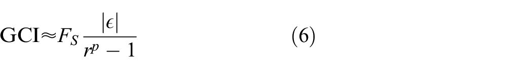
where
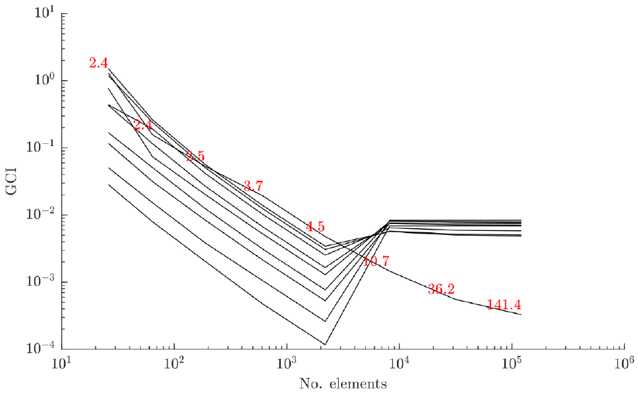
For the grid convergence analysis of the strut submodels, the diagonal (longer) strut was used in a cantilever setup. The nominal parameter values were used (Table 1), and no load or damage conditions were applied to the model. The results of this analysis are shown in Figure 6 (this plots the convergence of the first 10 modes of the strut, with solution times recorded at each grid point). This indicates good convergence of the modal analysis with increasing grid refinement for the first 10 natural frequencies of the strut. As shown in Figure 6, the optimum refinement for this component is around
The nominal parameters of the bridge substructures.
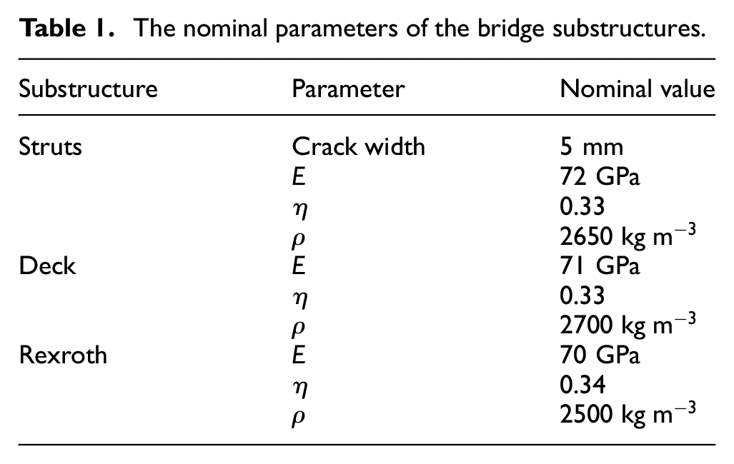
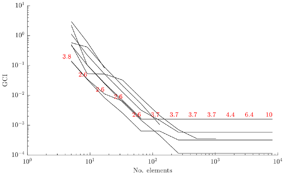
The GCI for the diagonal strut submodel, with solution times (in seconds) marked in red.
The GCI for the bridge’s upper frame submodel, with solution times (in seconds) marked in red.
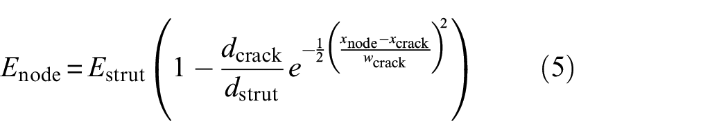
The GCI for the bridge deck submodel, with solution times (in seconds) marked in red.
The upper frame submodel consisted of five lengths of Rexroth beam joined to form a figure-of-eight, with free-free boundary conditions. This meant that the modal analysis produced six rigid-body modes, which were discounted from the analysis. The results are shown in Figure 7. This indicates good convergence of the modal analysis with increasing grid refinement for the flexural modes of the substructure. Based on the time taken to evaluate the model compared to its convergence, it is clear that the optimum number of elements for this substructure is around
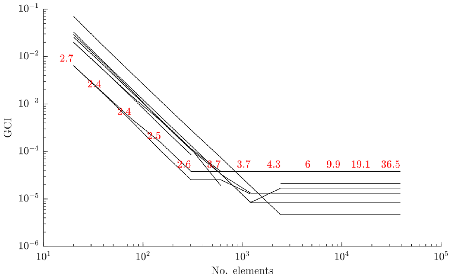
The deck submodel consisted of four lengths of Rexroth beam joined at the ends to form a rectangle, which bounded a thin rectangular plate. The submodel was fixed at each end, which replicated its boundary conditions as part of the bridge assembly. The results are shown in Figure 8. This indicates good convergence of the modal analysis with increasing grid refinement for the first 10 modes of the model. The optimum grid refinement for the deck substructure seems to be around
Following this grid convergence analysis, the element sizes were set to 11, 25 and 50 mm for the struts, upper frame and deck submodels, respectively. These were chosen by taking the element size at which the convergence for each substructure reached the asymptotic range and then doubling it to save on computational effort. This step back from satisfactory convergence would add some additional numerical uncertainty to the solution, but was required for this study to aid the timely development of the methods. Based on the verification activities summarised here in conjunction with many checks and code iterations, the numerical model implementations were considered accurate for following studies.
Experimental data: assembly level
The experimental data follows on from a similar dataset presented in 2021 to acquire undamaged- and damaged-state data from the bridge. 30
The 2021 tests were carried out in two phases. The first phase entailed a roving hammer tap test in order to identify the mode shapes of the structure under excitation in its nominal, undamaged state. This dataset was then used for matching the experimental modes to those predicted by the numerical model. The second phase entailed shaker-excited damage-state testing to identify the effect that increasing damage had on the natural frequencies of the structure. Damage was introduced by saw cut to the mid-point of each of the three vertical struts on one side of the bridge at 2.5 mm intervals up to maximum depth of 17.5 mm, at which point the strut was replaced before commencing the test on the next strut. The bridge was fixed at each end – with all DoFs constrained – to cast-iron mounts, which were in turn attached to heavy concrete blocks. These were considered to be rigid boundary conditions.
Similar tests were carried out for this case study, with the addition of a test to identify the impact of boundary condition uncertainty on the results. The first main objective of the new test set was to aid the accuracy of mode-matching by the modal assurance criterion (MAC) to the model predictions; this was done by carrying out a more high-fidelity roving hammer test with the bridge in its undamaged condition. The 2021 tests used 54 tap locations: 27 on the deck, one at the midpoint of each strut and 13 on the upper frame. 30 This was insufficient for providing mode shape data on which to discriminate between modes with similar mode shapes because the midpoint of the struts was a node for many mode shapes. In addition, the struts showed the most deviation in mode shape between modes and were the key components of interest, so additional tap locations along the struts were desirable. The present tests used 76 tap locations, with three locations excited along each strut at each quarter-length; the tap locations at the extreme ends of the deck were removed for these tests as the bridge was fixed at these locations.
The secondary objective of the new tests was to acquire a more globally descriptive set of damage-state data for the bridge; the damage tests were carried out on the struts that were symmetrically ‘unique’ in the structure, that is, the two diagonal and vertical struts located in one ‘corner’ of the bridge – these were the four struts in the far corner in Figure 2, closest to the laptop. These struts were labelled 1, 5, 2 and 6; see Figure 9. The present dataset should be more globally informative than the 2021 dataset as, due to the lines of symmetry of the structure in the
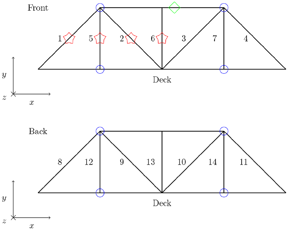
A schematic of the bridge structure, with damage locations marked in red stars, accelerometer locations marked in blue circles and the tap location marked in a green diamond.
The final aim was to investigate the uncertainty implications of the joints on the structure response. This was carried out by applying a known torque to the bolts fastening each strut to the assembly using a torque wrench, and carrying out repeat tests in between removing and reattaching a particular strut.
Methodology: healthy-state testing
Tap testing was used to identify the mode shapes for the lower modes of the bridge structure using the roving hammer method (the make and type of the impact hammer were PCB Piezotronics, model 086C03). This allowed for a large number of test points to be used without adding many accelerometers, which could impact the dynamic response of the structure. The ambient temperature was measured at
The dynamic response of the bridge was recorded in the range of 0 to 128 Hz. Reducing the scope of the tests to this frequency range had two benefits. Firstly, it allowed the use of an impact hammer with a very soft tip. This meant that double-impacts could be avoided, which were found to be an issue when exciting the struts due to their extreme flexibility. In addition to this, a frequency resolution of 0.0625 Hz could be achieved for the frequency response functions (FRFs). This in turn allowed for greater precision in identifying the natural frequencies within the spectra. This was desirable as many of the bridge’s natural frequencies were very close to each other in the frequency domain.
A triaxial accelerometer was used to record the response of the bridge to the impacts. This was attached to the Rexroth on the upper frame of the bridge, as the mobility of the structure was significant in that location, and many of the lower natural frequencies had mode shapes which involved displacement of this part of the structure. The accelerometer was fixed to the upper Rexroth on the near side of the bridge, between the first two joints in the x-direction; it is visible in Figure 2. The make and type of accelerometer were PCB Piezotronics, model 356B21.
Five repeat impacts were carried out at each damage location in order to reduce the noise in the results through averaging. Additional pre-processing measures to increase the cleanliness of the data was carried out by windowing the recorded excitation and response data.
Data acquisition was performed using the Siemens LMS system, with modal analysis carried out using the PolyMAX algorithm to isolate modal characteristics from the recorded FRFs. The final chosen modes were extracted concurrently with the modes used in the damage-state testing to ensure compatibility between the two datasets.
Methodology: damage-state testing
Tap tests were carried out on the bridge across a range of damage conditions using the same impact hammer as was used in the roving hammer testing. A single tap location was used with multiple accelerometers attached in the y- and z-directions at each joint (see Figure 9). The make and type of accelerometers were PCB Piezotronics, model 353B18. As with the roving hammer tests, repeats and windowing were used to reduce the noise level in the recorded data.
The ambient temperature was measured at
Damage was introduced to struts 1, 2, 5 and 6 by saw cut at the midpoint at 2.5 mm intervals, up to a maximum ‘crack’ depth of 17.5 mm. When each damage run was completed the strut of interest was replaced with a new strut. The damage locations and tap location are illustrated in Figure 9.
The final tests were carried out immediately after the damage-state testing. Strut 1 was removed and reattached three times, with tap tests carried out following each reattachment. This was in order to assess the uncertainty caused by the boundary conditions and provide a number of test points describing the bridge in its normal condition. The methodology was otherwise the same as for the damage state testing, described above.
Results
The FRFs were stored for each of the above-described test sets, from which modal data was extracted using the PolyMAX curvefitting algorithm. This method utilises a numerical approach to isolate the natural frequencies, damping ratios and mode shapes from manually selected resonance peaks on the FRFs. The key parameters guiding this process are the tolerances set for the natural frequencies, damping ratios and mode shape vectors for each peak, the maximum number of DoFs allocated to the curve fit, and engineering judgement. These tolerances describe the stability of a modal fit for a given resonance peak, where the solution would be considered stable if it was within each tolerance criterion when compared to the solution with one fewer DoF. The tolerances set for this analysis were 0.1% for the frequency, 5% for the damping ratio and 0.5% for the mode shape, meaning that the exported solutions are accurate to these boundaries. These values were set to tightly control the extracted natural frequencies, as these were of interest as features in the following analyses. Following feature extraction, the datasets were matched to each other using the natural frequency values, which resulted in an experimental dataset of 18 natural frequencies for each test.
Feature selection
The aim of feature selection at this stage of an FMD-SHM strategy using hierarchical validation is twofold: firstly, a set of damage-sensitive features that can be used to train a statistical model for damage detection in real-life structural data is required; secondly, a set of features on which it is appropriate to validate the submodels which make up the assembly should be identified. The features generated by the assembly-level model to train the statistical model for damage detection should be selected based on their variance when the input damage to the model is varied (where large observable variance is preferable). The features selected on which to validate the individual strut models must exhibit sensitivity to damage in order to allow for the damage model to be validated at this level. Engineering judgement must be exercised to ensure that the validation features at the substructure level are relevant to the selected features at the assembly level.
Natural frequencies were identified as suitable features for use in this study, due to their low dimensionality. In addition to this, the natural frequencies can be shown to be sensitive to global damage in structures and substructures and are therefore appropriate to hierarchical model designs, as they can be expected to indicate damage at both the assembly and substructure level. Finally, a key advantage to the use of natural frequencies as damage-indicating features is that they require few sensors in order to measure, provided that the sensors are not placed on any significant nodes of the structure. A key drawback of using natural frequencies as features in vibration-based SHM is that they do not give good information on damage location compared to other features such as mode shapes.
The feature extraction process for the model predictions in this case study was carried out by finding the eigenvalue solution to the model’s equation of motion. Extracting the natural frequencies from the experimental data was carried out using the PolyMAX curvefitting algorithm to the FRFs of the structure.
Feature selection was carried out in this study by using the physics-based model prior to validation to identify which of the extracted features – proportional changes in natural frequencies – were sensitive to the damage states of interest. The parameters of the model were its material parameters and the crack width, which are summarised in Table 1.
The first stage of the feature selection process was to use the model to generate a set of natural frequency predictions across the full range of damage. The damage states were midpoint cracks in each of the struts, ranging from the healthy condition to a crack depth of 17.5 mm at intervals of 2.5 mm. The first 50 natural frequencies were predicted using the model, which ranged up around 100 Hz.
Of each of these natural frequencies, the MAC was used to assess which modes remained ‘stable’ across the full range of damage – that is, which natural frequencies kept a consistent mode shape throughout the described range of inputs and did not switch with other modes as damage progressed. The threshold for the MAC below which the modes were considered to have changed significantly was set to 0.9. The majority of the predicted modes satisfied this criterion and were therefore retained for further analysis. Ensuring that the modes remained comparable to each other across the full range of damage meant that they could be expected to retain a fit to the experimental data, across damage conditions, after being matched to data from the structure in its undamaged state.
Following selection of the subset of ‘stable modes’ from the model predictions, mode-matching between these predictions and the experimental data was required. This was carried out by using the MAC to assess the similarity between the experimental and predicted mode shapes and by comparing the predicted natural frequencies with the experimental data. Given that there were many more predicted modes than were extracted from the experimental data, the matches were then finalised by selecting matches that maximised the MAC and minimised the error between the predicted and the experimental natural frequencies. The MAC was set to a minimum of 0.5 and the error between natural frequencies set to a minimum of 10%. This yielded a further reduced subset of modes.
Based on the criteria above, differing numbers of features were matched to the experimental data based on the number of available ‘stable’ modes from the first stage. The matched modes were then fed back into the model in order to determine which showed the most sensitivity to damage in each strut. The sensitivity was assessed by finding the percentage difference in natural frequency as damage progressed compared to the undamaged natural frequency for a given mode. Two modes were then selected for each strut. This selection was carried out by ordering the modes by their sensitivity at the highest level of damage and discarding the half of the feature set that was the least sensitive. Following this, the two modes with the highest MAC were selected from each remaining subset. Further selection criteria could be applied at this point, such as tests for feature robustness to environmental and operational variables (EOVs), as was investigated in Wilson et al. 14 The resulting subset of modes for this analysis are shown in Table 2.
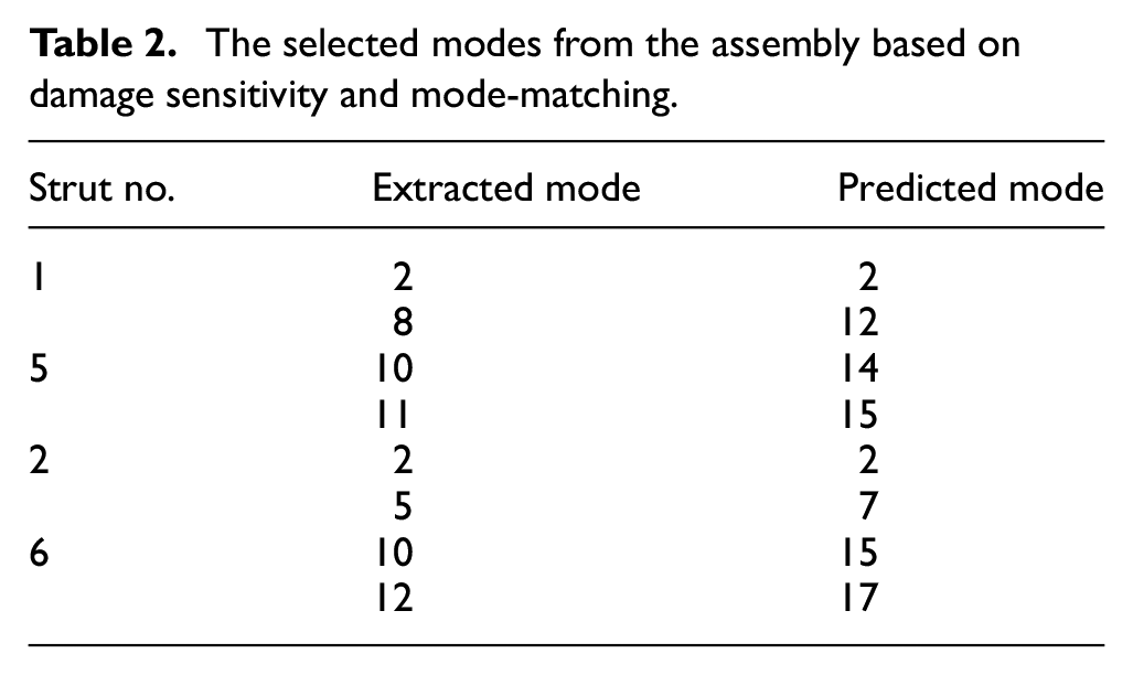
The selected modes from the assembly based on damage sensitivity and mode-matching.
Having determined a set of candidate features at the assembly level, it was required to determine a similar feature set on which to validate the strut models. Given that the first few natural frequencies of the struts in isolation covered the full range of frequencies extracted from the bridge, these were considered a reasonable feature set for submodel validation. To ensure that the modal behaviour was comparable between the struts in isolation and the struts when built into the assembly, a mode-matching was carried out between the two cases using the MAC. A key difficulty in this was that the main local mode shape for the struts in the assembly (at the lower modes) was an s-bend as the upper Rexroth was displaced. This was not captured in the isolated strut model, as the strut was constrained at both ends. Nevertheless, it was found that the first five natural frequencies of the struts in isolation could be loosely matched to the first hundred modes of the assembly, and would therefore be suitable for validation in this case.
The candidate validation feature sets (first five natural frequencies) for the two strut submodels are plotted in Figure 10. The features plotted are the proportional changes in the natural frequency as the damage progresses. Sensitivity to damage is clear, which means that these features will be suitable targets on which the validate the predictive damage models in the strut submodels; the use of these modes in validation is contingent on the ability to match them to experimental data.
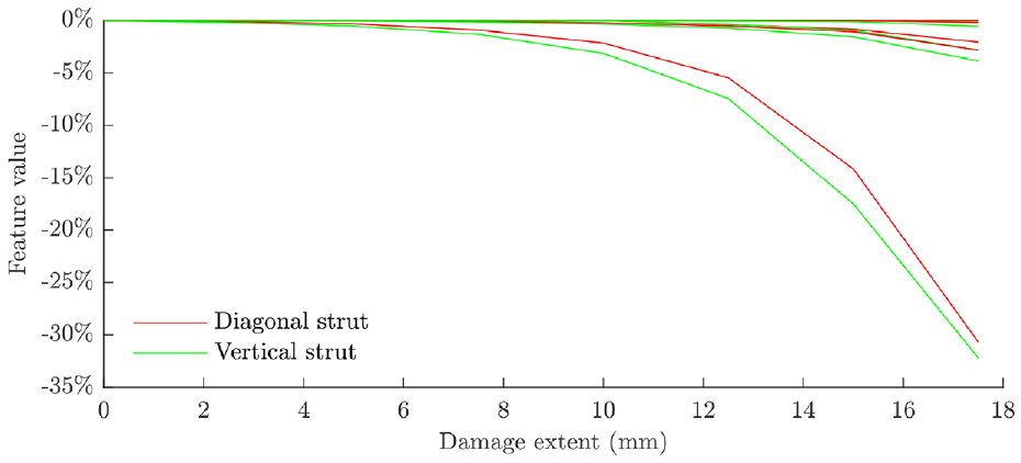
The features selected on which to validate the diagonal and vertical strut submodels for damage prediction.
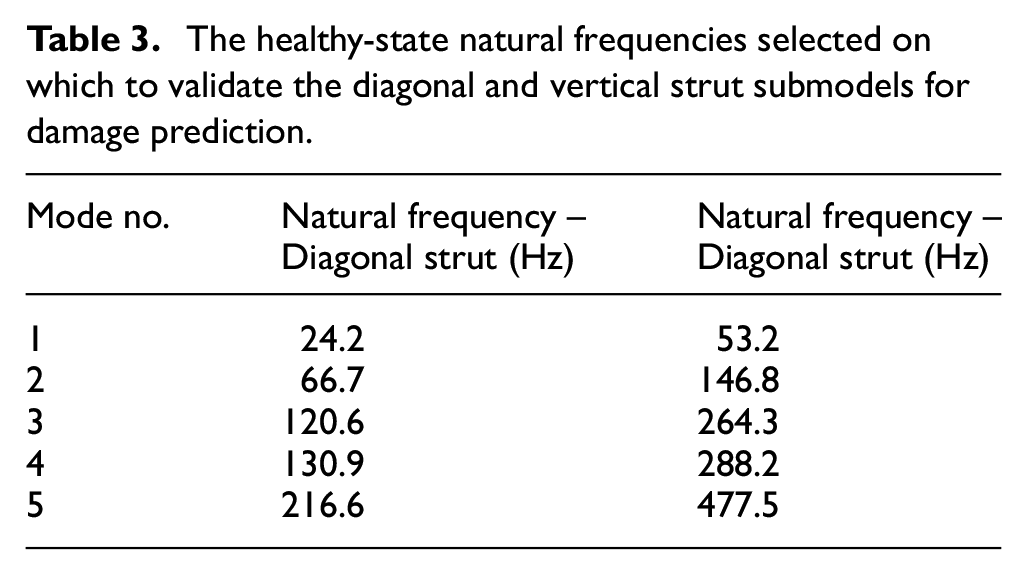
The natural frequencies selected are given for each strut in its undamaged condition in Table 3. The third mode was the most sensitive to damage and can be seen to be significantly more sensitive than the others in Figure 10. This is the first bending mode for both struts in the same dimension as the crack length, which explains the strong sensitivity to crack growth.
The healthy-state natural frequencies selected on which to validate the diagonal and vertical strut submodels for damage prediction.
Damage model validation
In order to attain an assembly-level predictive damage model of the bridge, the individual strut submodels were validated against experimental data. This entailed calibration of the material parameters of the submodels, and calibration, selection and validation of the crack models within the strut submodels. The validation process should allow quantifiable confidence to be attached to further predictions in the implementation of the model, which could then be used to make predictions at the assembly level with associated confidence via dynamic substructuring.
Experimental data: component level
The struts were tested under a range of static load conditions and damage scenarios. Both the vertical (shorter) and diagonal (longer) strut types were tested. The strut was fixed to a relatively rigid cast iron base structure, which itself set on damped steel feet. The strut was clamped at the top end with all DoFs fixed. At the bottom end, the strut was fixed to a runner such that all DoFs were fixed except for movement parallel to its length. Static loads could be applied to the strut by means of a pinion and wheel. The loads were controlled using weights that applied a moment to the wheel, which in turn applied vertical load to the pinion. This vertical load was tracked by a load cell. The rig is shown in Figure 11.
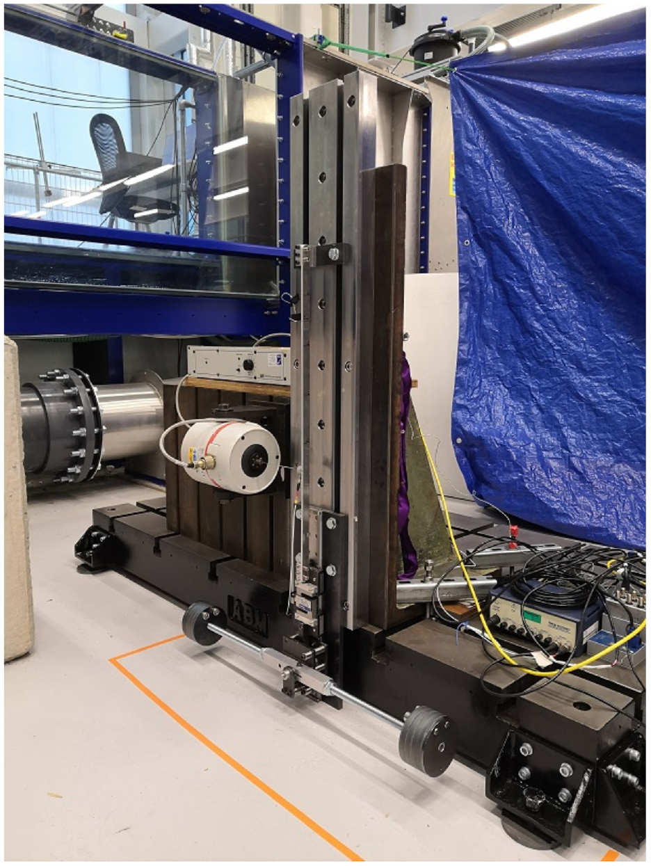
The rig used to conduct validation tests on the bridge struts with load mechanism at bottom end of strut and shaker shown attached; laser vibrometer not shown.
The struts were fastened to the mounts using bolts tightened to a torque of 10 Nm. A piezoelectric shaker was used to excite the struts via a stinger with a PCB 208CO2 force transducer; the shaker was attached to the same rigid structure as the strut and used a white noise signal ranging from 0 to 1000 Hz. The stinger was attached to the strut away from the measurement locations and away from any significant integer divisions along the strut length in an effort to avoid any mode shape nodes. The strut response was captured using a scanning laser vibrometer. The vibrometer measured the strut accelerations at a rate of 2560 Hz; a total of 32,768 samples were taken for each measurement point.
On the diagonal strut, 18 measurement points were recorded at 100 mm intervals (measured from the top end of the strut). At each vertical location two points were recorded, on either side of the central longitudinal axis of the strut. For the vertical strut, 22 points were recorded at 50 mm intervals.
The tests on the strut in the undamaged condition showed that the application of the static load has a noticeable effect on the dynamic response of the strut. Similar sensitivity was observed in the results for the vertical strut, indicating that the strut models should be validated against a range of static load conditions in order to capture any boundary condition loading they would experience in the full assembly.
Damage was added by saw cut incrementally to each strut through testing. In the diagonal strut, it was introduced at
Mode-matching was required in order to ensure that the features being validated from the numerical predictions were being compared fairly to their equivalents found in the experimental data. The first 10 and 8 predicted natural frequencies by the model were generated for the diagonal and vertical struts, respectively (the number of predicted modes in the range 0–1000 Hz for each strut). These were generated under each load case for each strut taken from the experimental conditions.
Given that the experimental data recorded the response in the z-direction only, it was to be expected that fewer modes would be identifiable in the same frequency range than would be predicted by the model. Due to the well-separated nature of the natural frequencies in this range of the frequency spectrum, it was possible to make the following matches using the comparison between the predicted and experimental natural frequencies. Analysis of the predicted mode shapes at these frequencies showed that these modes did have mode shape displacements in the z-direction, and the MAC indicated that the matches were legitimate based on these mode shapes (although certain estimates of the MAC were very low due to measurement noise on the experimentally derived mode shapes and the low displacement of certain modes). This led to the following set of matched modes (Table 4).
Summary of the matched modes between the experimental data and model predictions.
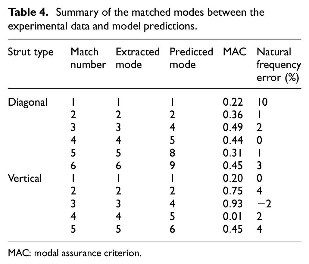
MAC: modal assurance criterion.
The first five predicted modes had been identified as ideal for validation in the feature selection stage; however, these could not all be reliably matched to experimental data, as can be seen from Table 4. Where matches could not be found from the first five predicted modes, higher modes were used in their place.
Calibration of material parameters
Calibration of the strut models in their undamaged condition was carried out in order to determine the uncertainty in the material parameters of the models and to ensure the accuracy of their predictions. The calibrated strut models could then be used in the validation of the damage models applied to both struts, which would allow for confidence to be established in the predictions of the models under damage conditions. The material parameters of the strut models were Young’s modulus, density and Poisson’s ratio (the nominal values for these are given in Table 1).
Calibration was carried out by minimising the error between the predicted and experimental values for the first four matched modes of the vertical and diagonal struts. The material parameters of the two struts were assumed to be represented by the same underlying distributions, given that the components were cut from larger sheets of the same aluminium plate. Previous analyses of the bridge under static loading showed that the struts would experience a range of static loads in operation of the bridge, both compressive and tensile (along the length of the struts), so the calibration was carried out at a range of static loads. The distribution of the parameters was estimated by fitting a normal distribution to the values derived by using the Nelder and Mead Simplex algorithm – an unconstrained multivariate optimisation process – at each load point and each strut. 31
Initial attempts were made to calibrate the Young’s modulus and density of the struts concurrently, with the Poisson’s ratio assumed to be relatively accurate (and also to have negligible impact on the results). However, this caused issues as the relationships between the target features – natural frequencies – and the two calibration parameters were inverses of each other. Therefore, the final calibration was carried out on the Young’s modulus of the struts only, and the Poisson’s ratio and density were kept at their nominal values.
It should be noted here that for an ideal calibration process, a bespoke design of experiments would be carried out prior to experimental data acquisition. This would use multiple struts in tests designed purposely to measure the quantities of interest in order to form a relatively large distribution. For example, a set of static load tests on a large set of struts could have been used to measure the Young’s modulus, and another set of struts could have been weighed in order to measure the material density. In this set of tests, only two struts were used: one vertical and one diagonal. The vibration data recorded was intended for validation of the dynamic damage models and was not particularly suitable for material parameter calibration. This limited the capability of the calibration process; however, as is shown below, some improvements were made on the estimation of the model parameters.
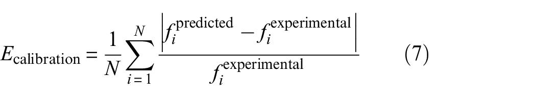
The error function for the optimisation algorithm was the mean of the error magnitude between the first four predicted and experimentally derived natural frequencies (Equation (7), where
The results of the optimisation process for calibrating the Young’s modulus of the struts.
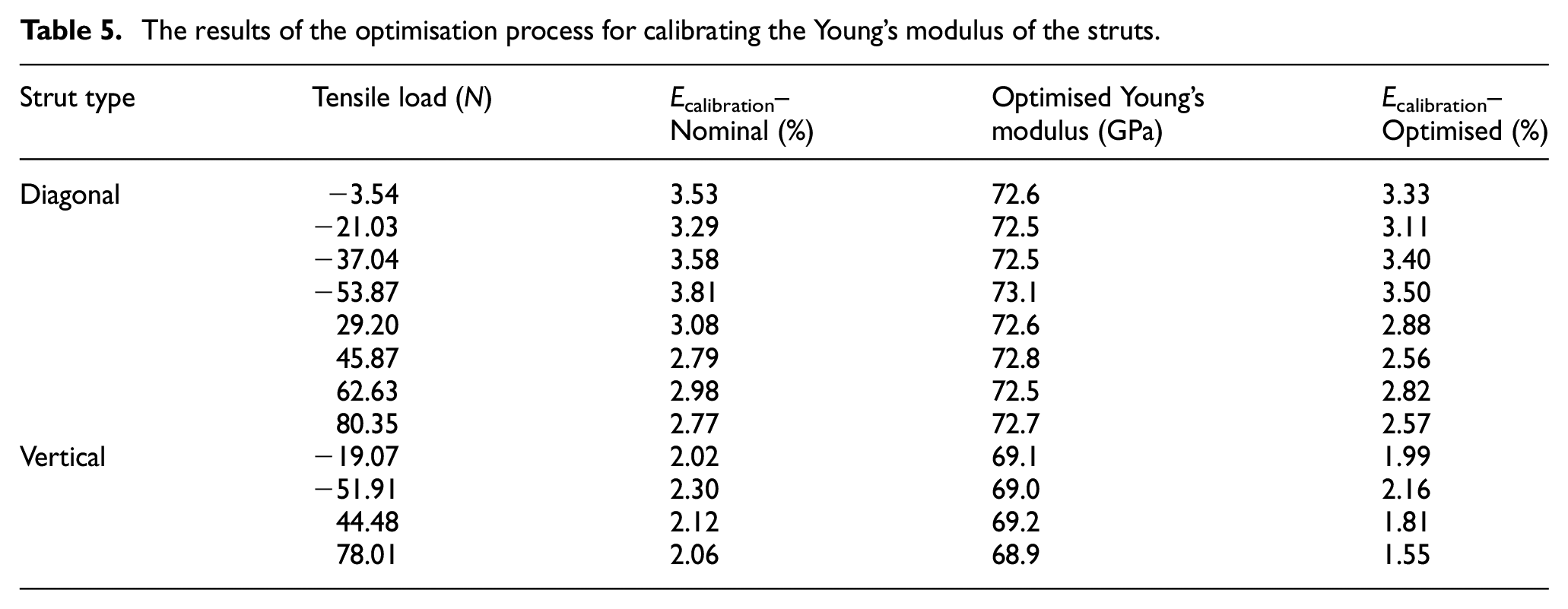
The underlying distribution for the Young’s modulus was estimated by fitting a normal distribution across all the test points; the form of the parameter distributions was based on the assumption that the central limit theorem would hold in a large population of components. Other distributions may perform differently; this would require separate investigations to the present works. The mean and standard deviation fitted to these results were 71.5 GPa and 2.52%, respectively. When these values were validated against the fifth natural frequency for each strut, which was left out of the calibration process, the error was comparable in magnitude to the error for the previous modes, which gives validity to the calibration process (see Table 5). Therefore, these results were used as the basis for further work.
Damage model parameter calibration
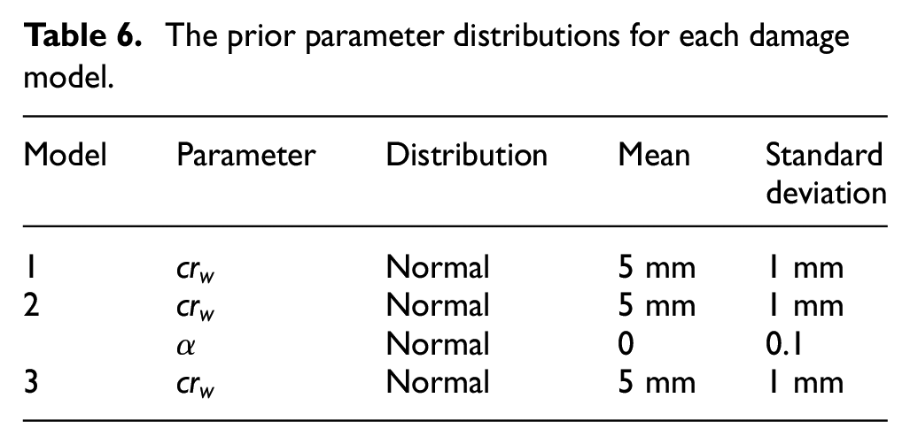
The parameters of the damage models were calibrated using approximate Bayesian computation (ABC). 32 This algorithm draws samples of the model parameters from a set of prior distributions, and then tests the models based on the samples against experimental data. An error metric is defined such that any sample points that produce an error greater than the threshold on this metric are discarded, while those that produce a lower error are retained and used to form an estimate of the posterior distribution. This makes ABC a likelihood-free method for estimating the posterior distributions of model parameters. ABC was selected for this research as it removed the task of fitting a formal likelihood distribution to the experimental data while enabling the incorporation of prior knowledge on the model parameters. The prior parameter distributions for each model were set according to Table 6.
The prior parameter distributions for each damage model.
The models were tested at a range of load points and damage conditions, with certain damage cases left out in order to validate the results of the ABC process for each model. The test points used for each set are summarised in Table 7.
The test points at which the experimental data was recorded for each strut.
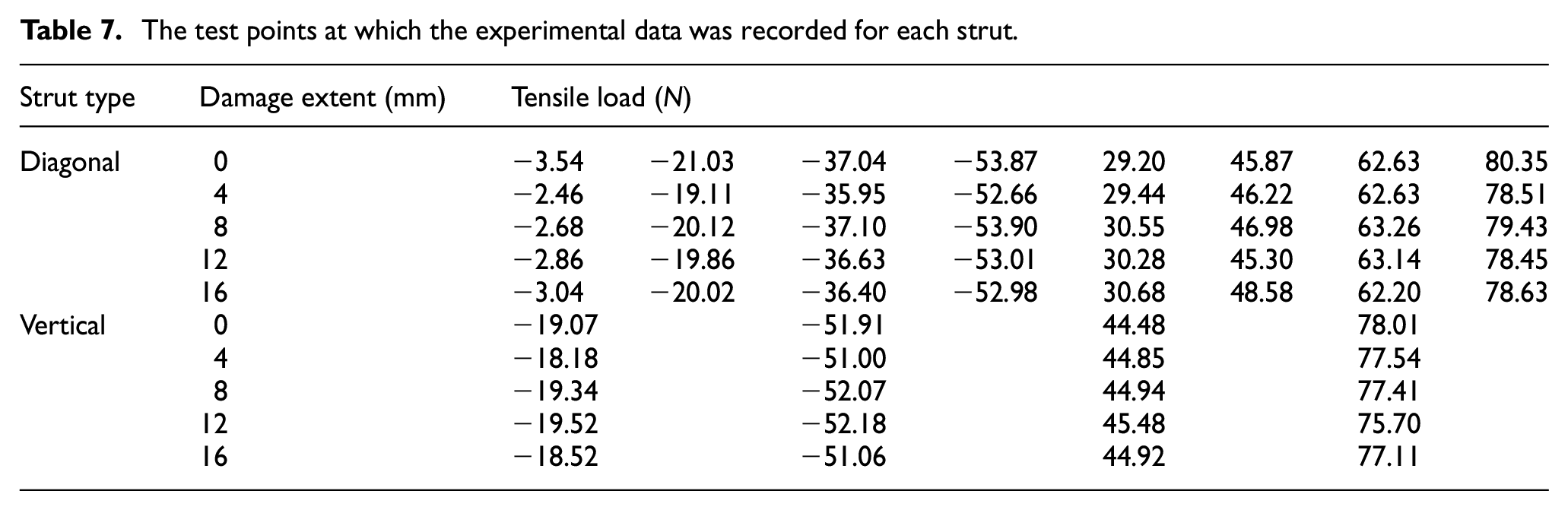
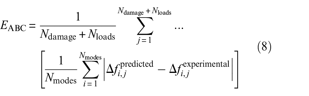
The training set utilised the proportional change in natural frequency from the undamaged condition at damage extents of 8 and 16 mm, whereas the validation set used the same feature at 4 and 12 mm. The error function upon which the threshold for the ABC posterior estimation was set was the average of the difference between the predictions and experimental data at the damage extents across all damage and load cases, and across the first five matched modes (as described in Equation (8)).
The acceptance rates for the three models based on this error metric for prior distributions of 1000 samples are given in Figure 12. This indicates that model 3 performs the best of the three considered models, with model 2 slightly out-performing model 1. In order to allow for fair comparison between the posterior distributions estimated for each model, a minimum acceptance ratio was set at 10%. This yielded the posterior parameter distributions shown in Figures 13–15. Models 1 and 3 yielded highly skewed posterior distributions for the crack width parameter; as this was the only tuneable parameter for these models, the nature of ABC means that one tail of the prior will be selected which causes skewness in the posterior. Model 2 has two parameters, which allows for a less skewed estimation of each. In each case, the posterior distributions contained crack widths from the higher end of the prior distribution, indicating that the prior model underpredicted the sensitivity to damage in the struts (the
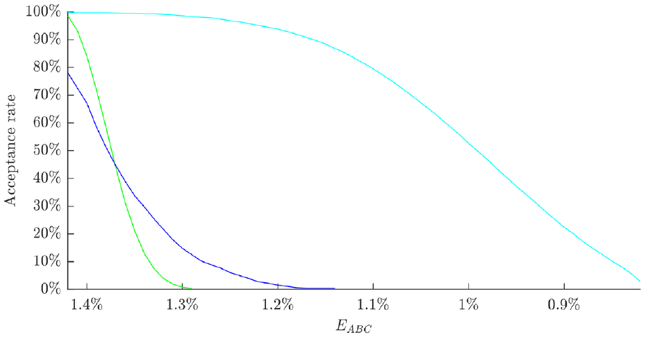
ABC acceptance rates for model 1 (green), model 2 (blue) and model 3 (cyan).
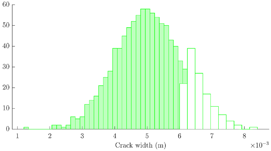
Histograms of the prior (filled) and posterior (clear) of crack width for model 1.
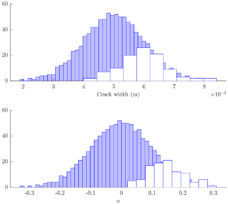
Histograms of the prior (filled) and posterior (clear) of crack width and
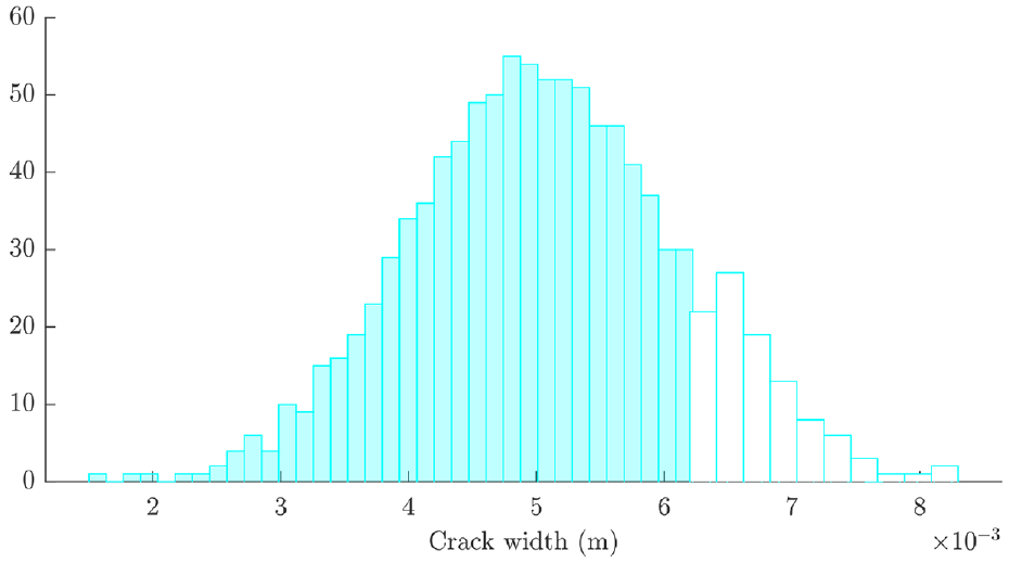
Histograms of the prior (filled) and posterior (clear) of crack width for model 3.
Posterior validation
The damage extents of 4 and 12 mm were left out of the error function for estimating the parameter posteriors in order to provide validation data for the ABC results. The prior and posterior parameters were evaluated at these test points in order to validate the ABC process carried out at the other test points. Ten samples were taken from the prior and posterior datasets for this process. These samples are plotted across the damage range in Figures 16 to 18 for the vertical strut for each of the models. It is clear from these that some improvement in accuracy has been made; however some inaccuracies remain, which are particularly noticeable at higher damage extents. Notably, the predictions are clearly highly robust to the static load conditions that the struts were subjected to for all modes and damage models.
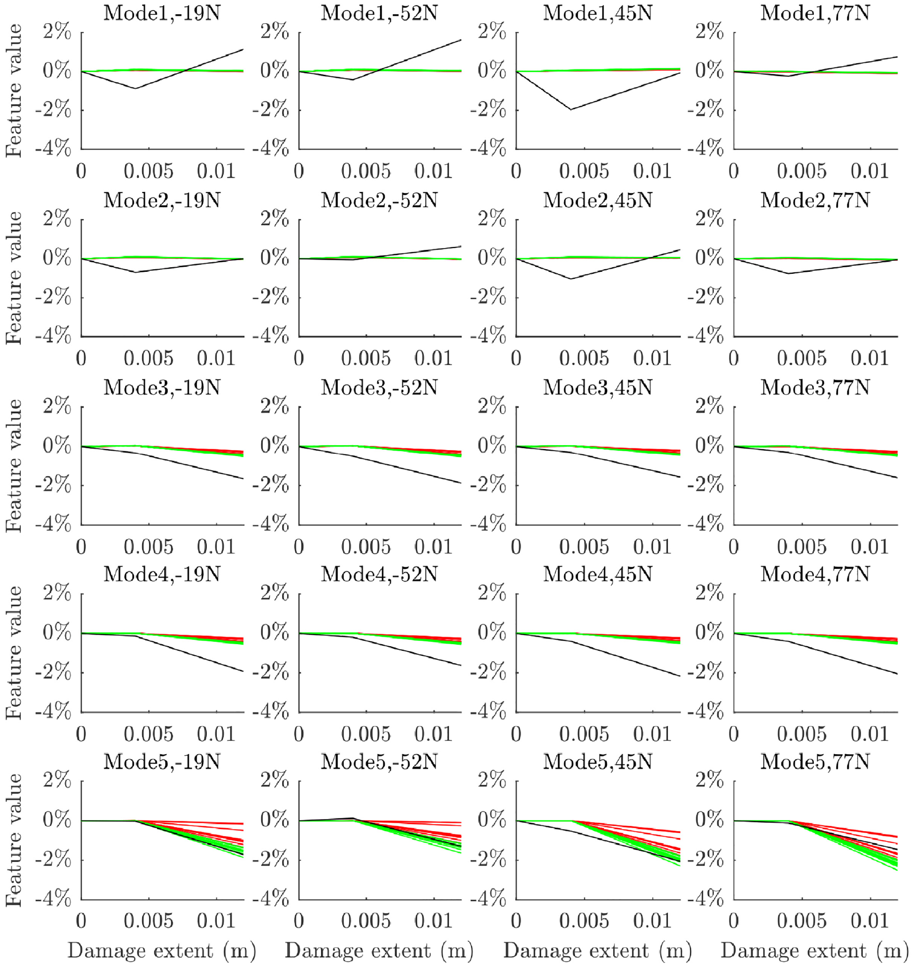
The change in natural frequency at the validation test points for the vertical strut with experimental data in black, prior samples in red and posterior samples in green for model 1.
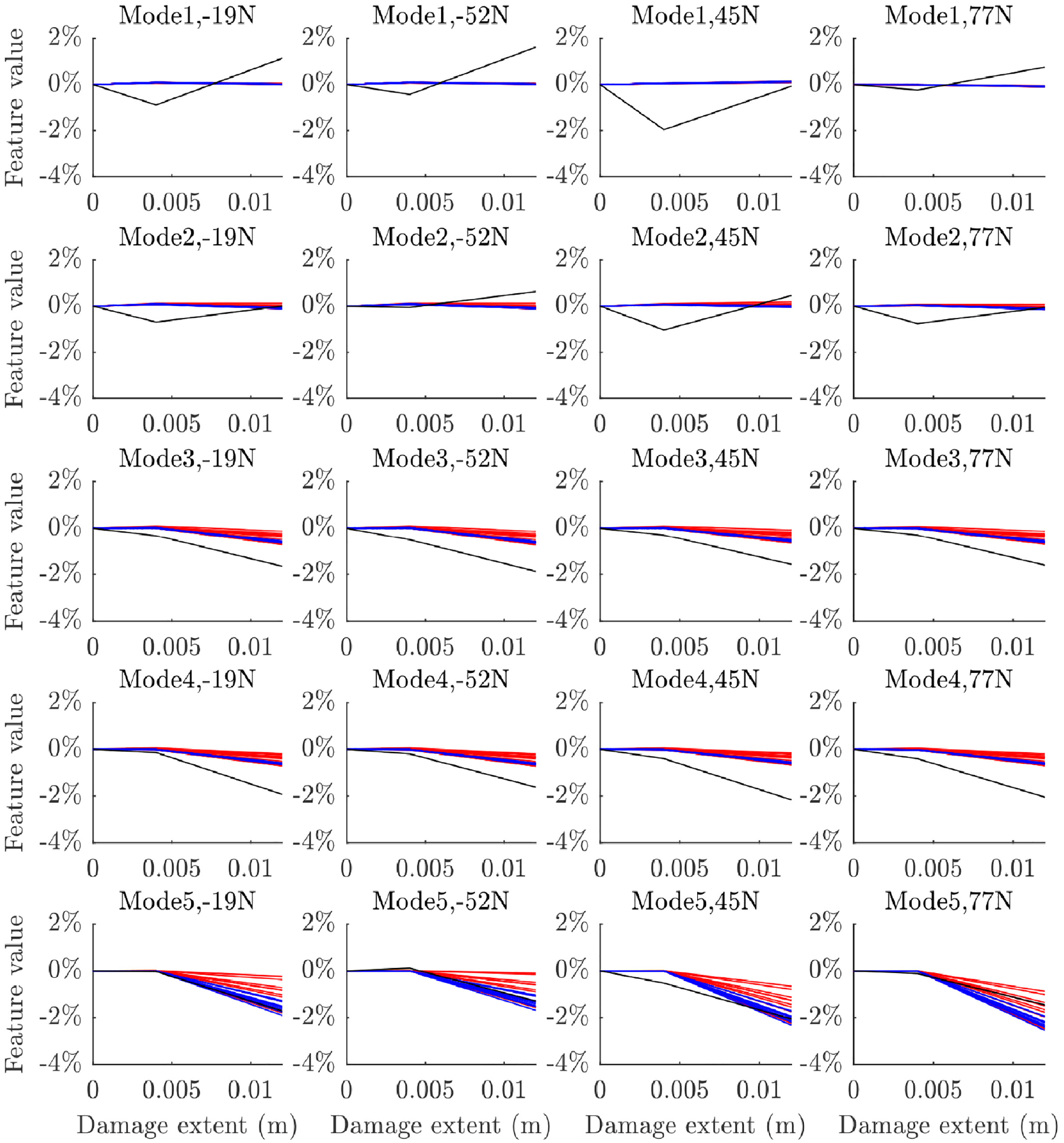
The change in natural frequency at the validation test points for the vertical strut with experimental data in black, prior samples in red and posterior samples in blue for model 2.
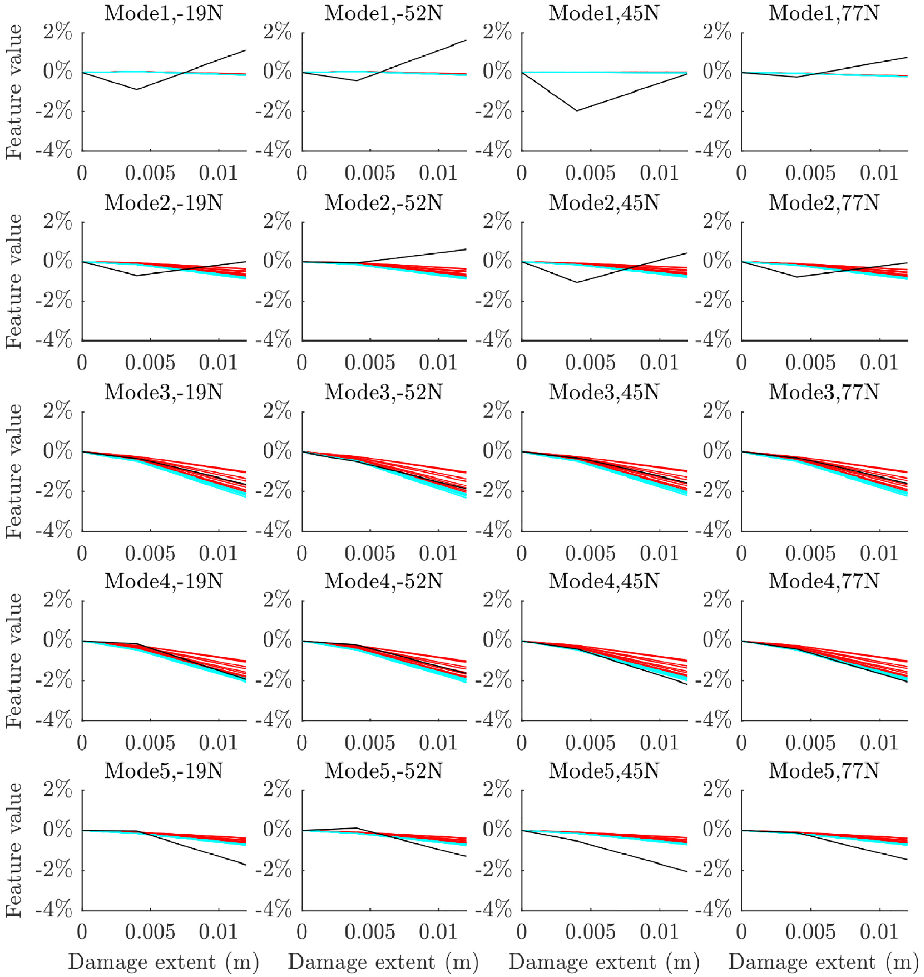
The change in natural frequency at the validation test points for the vertical strut with experimental data in black, prior samples in red and posterior samples in cyan for model 3.
Model 1 clearly does not capture the full sensitivity to damage for modes 3 and 4, however the posterior does offer a more accurate set of predictions than the prior model in this case. The same can be said for model 2, which seems to provide a greater estimate of the uncertainty on its predictions. Both models predict the fifth mode well and capture the lack of damage sensitivity on modes 1 and 2 (although the level of uncertainty on these modes does not seem to have been fully quantified given the variation seen in the experimental data for these modes). Model 3 performs better than models 1 and 2 when predicting modes 3 and 4, but is comparatively less accurate when predicting mode 5. Model 3 captures sensitivity to minor damage much better than models 1 and 2, which tend to underpredict damage sensitivity at crack depths of 4 mm. Like models 1 and 2, model 3 captures the lack of damage sensitivity in modes 1 and 2, but seems to do a better job of robustly quantifying the level of uncertainty on mode 2.
Based on the calibration and validation tasks carried out at the substructure level in this section, model 3 would be selected for use at the assembly level. However, all three validated models were tested at the assembly level in order to investigate if the conclusions drawn from testing at the substructure level would prove accurate at the assembly level. The validation can be considered an initial success, as it avoided the use of damage-state data at the assembly level, drawing this instead from the struts in isolation. If this can be shown to be impactful on the model predictions at the assembly level, this will demonstrate the potential for hierarchical validation within an SHM context.
Uncertainty propagation
Uncertainty propagation was carried out in conjunction with the model assembly process following the previous submodel validation activities in order to allow assembly-level predictions to be made with the associated uncertainty that was quantified through validation. The outcomes of the validation process were a set of posterior distributions for the parameters of the three strut-level damage models. These were incorporated into the assembly-level model of the bridge via dynamic substructuring directly. In addition to this, the uncertainty quantified on the material parameters of the struts in calibration was applied to the undamaged struts in the assembly by drawing samples from the material parameter distributions.
The full assembly model was generated from a set of pre-written submodels via primal dynamic substructuring in the physical domain. This was carried out under the assumption of rigid joints between the substructures at the nearest node location in the submodels. The rigid-joint assumption is not accurate for this structure: the joints actually contained a set of non-rigid bracket components. These components were neglected from the model; their mass and stiffness contributions would lead to some model discrepancy in the assembly model. However, this was assumed to be relatively insignificant to the model predictions. Other inaccuracies in the assembly include the geometric discrepancies caused by assuming that the struts were fixed directly at their extremities to the deck and upper frame.
The inputs to the model were the damage extents, the strut at which the damage was located, and the location of the damage along the strut. For each set of inputs, a full set of struts were generated of the same length as the posterior distribution of the damage model parameters. The strut containing the damage was assigned the crack model parameters and material parameters from the posterior distribution, whereas the remaining struts were assigned material parameters sampled randomly from the distributions estimated during calibration using Latin hypercube sampling. These submodels were then coupled with the nominal submodels of the deck and upper Rexroth (which had not been calibrated or validated – another unquantified source of uncertainty) to create a set of assembly models of the same length as the damage model posterior. This allowed, for a given set of inputs, a stochastic set of model predictions for those inputs.
The predictions across the damage extents are plotted against experimental data for the three validated models and their nominal equivalents in Figures 19 to 21. The features of interest were identified earlier in this paper, with two features identified as being sensitive to damage in each strut (see Table 2). There are two immediate findings that can be taken from these plots. The first is that a significant leap in accuracy was not achieved in validation, although some improvement is clear for certain cases (e.g. the predictions for damage in strut 5 using model 2 or strut 1 using model 3). The second is that validation allowed for good quantification of uncertainty in the assembly-level model predictions – this is informative when employing the model without assembly-level test data. Very low sensitivity can be observed for model 3 on the second feature for strut 2 (see Figure 21; differentiation between the model predictions and experimental data is difficult due to their similarity); this indicates that the selected feature would not be very appropriate for SHM applications and reselection following validation may be required. On the other hand, it is pleasing that insensitivity in the experimental data for this feature is mirrored in the model predictions before and after validation.
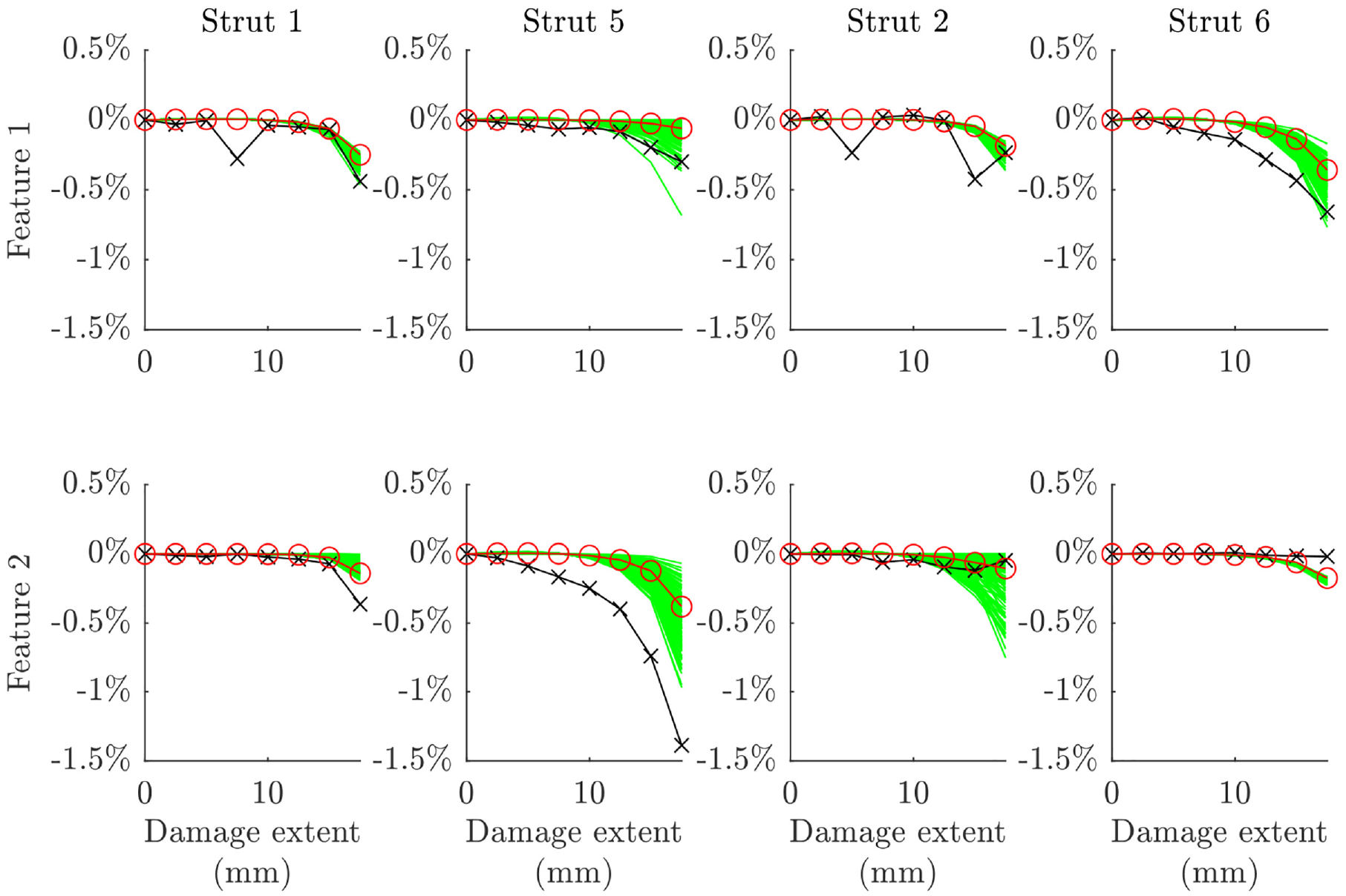
Predicted features at the assembly level compared to experimental data (black x’s) for the nominal (red o’s) and validated (green) parameter sets for model 1.
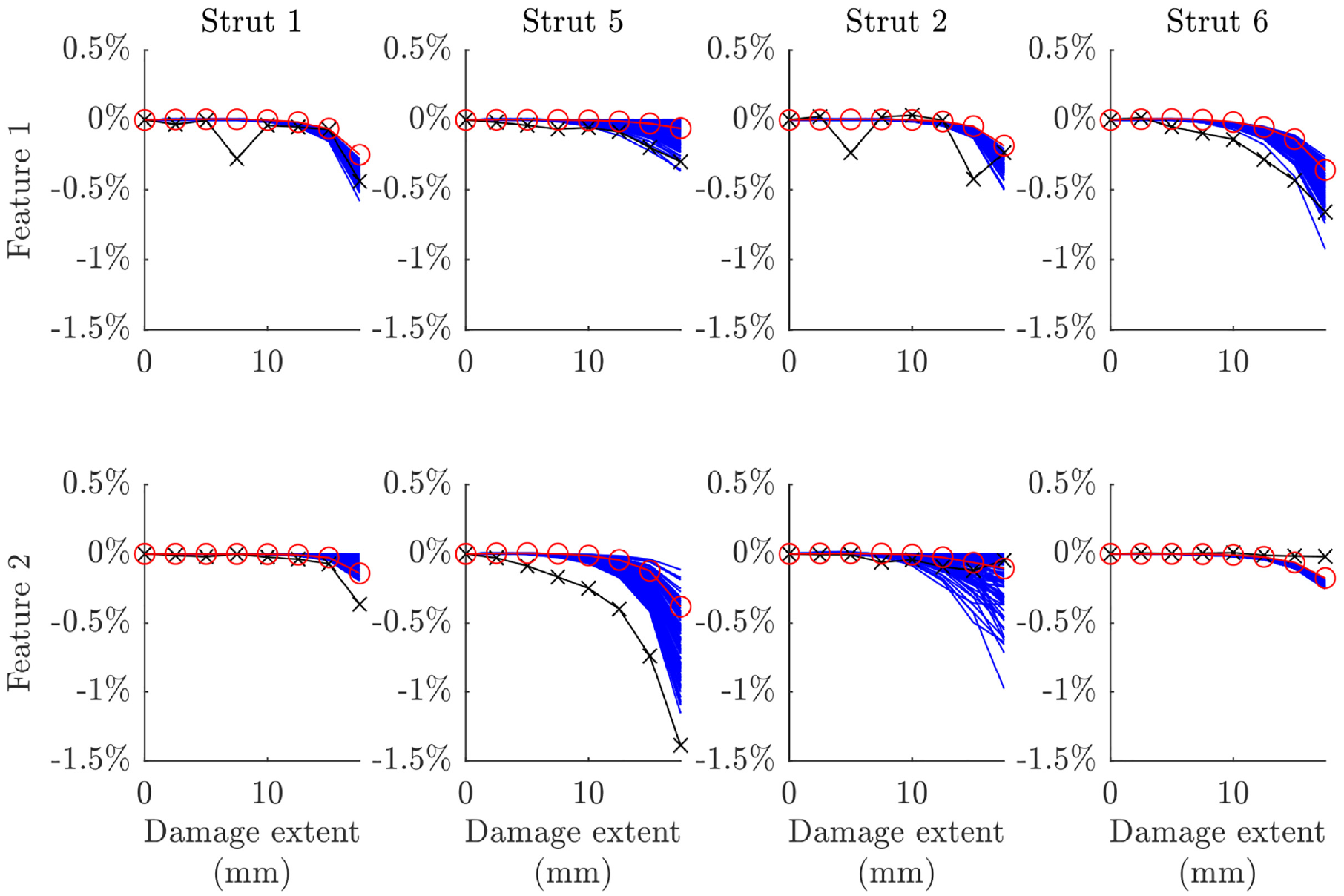
Predicted features at the assembly level compared to experimental data (black x’s) for the nominal (red o’s) and validated (blue) parameter sets for model 2.
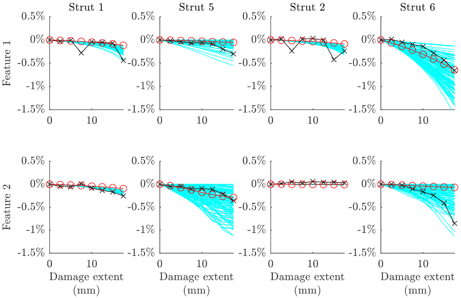
Predicted features at the assembly level compared to experimental data (black x’s) for the nominal (red o’s) and validated (cyan) parameter sets for model 3.
Model 3 appears to be the most accurate of the crack models investigated, followed by model 2. This confirms the predictions made at the substructure level and lends credibility to the hypothesis that validation and model selection activities carried out on assembly submodels can be used to confer validity of the assembly-level model. The accuracy of the models is further tested by applying their predictions in an FMD-SHM strategy in the following sections.
Damage detection
Damage detection refers to the task of determining whether data drawn from a structure indicates the presence or lack of damage in the structure. Damage detectors can be trained using either supervised or unsupervised learning processes, while localisation or assessment tasks generally require a supervised learning process (where the labels would be attached to potential damage labels or extents respectively). The output of labels based on features within recorded data – in an SHM context – allows engineers to make informed decisions on the management of a structure, for example to continue operations, to schedule an inspection or to take the structure out of service. These decisions are often enhanced by developing processes to analyse the risk attached to various classifier outputs; this can be done by using various cost functions bespoke to the application.
Damage detection methodology
Classification refers to the act of assigning a label, which signifies membership of a particular class, to a particular datapoint; in the field of SHM this usually means to take a data feature such as a natural frequency and to label it as being recorded from a structure in a particular health state (such as the undamaged or damaged classes in damage detection). The algorithms that carry out this task are called classifiers and can be trained using machine learning techniques. These techniques can be separated into supervised and unsupervised learning processes. Classifiers that are trained by an unsupervised process learn the class of a particular set of data; when exposed to fresh data, they are then able to distinguish whether or not it came from the original class of data. Classifiers trained by a supervised process are exposed to labelled data from at least one class; they should then be able to assign fresh data to one of the classes they have learned.
Two key types of classifier models are discriminative and generative classifiers. Discriminative models aim to use the training data to learn the boundary between two sets of labelled data, and are therefore often suited to supervised learning methods. 33 Generative classifiers, on the other hand, attempt to infer the probability distributions that the datasets are drawn from; they are therefore often applied to unsupervised learning problems. 33
A further important pair of classifier types are probabilistic and deterministic classifiers. 34 Deterministic classifiers refer to methods that will always label a particular data point to a particular class, whereas probabilistic classifiers will assign a particular data point a probability of membership to each class. The deterministic classifier is therefore often quicker and easier to use, but probabilistic classifiers can be more informative, particularly in a risk-based context.
Support vector machines (SVMs) are powerful tools for binary classification. They are based on a discriminative method and are non-probabilistic by nature. They can be used to produce a probabilistic output using the Platt method 35 ; this proceeds by fitting a sigmoidal probability function to the scores returned by the classifier rather than simply classifying them by some particular threshold. They can also be extended to multi-class classification tasks by using multiple binary classifiers to separate different regions of the feature space.
SVMs function by attempting to maximise the margin between two classes of data, where the margin is the perpendicular distance from the decision boundary to the nearest datapoints (support vectors) on each side. The form that the decision boundary takes is governed by the kernel; widely used options include linear, polynomial and radial basis function (RBF) kernels. The choice of kernel dictates the parameters that are adjusted to maximise the margin; for example for a linear kernel, the decision function would take the following form:

In this example, the (binary) classes are denoted by
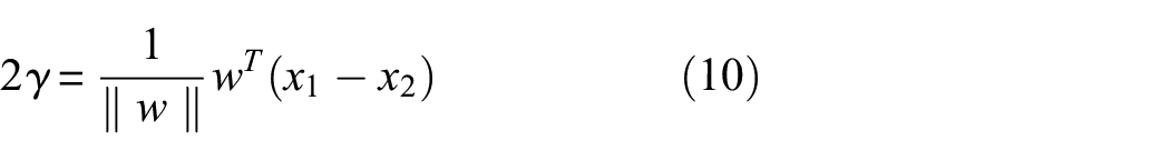
Given that Equation (9) yields a binary output, the argument is invariant to linear scaling and can be fixed such that the output is
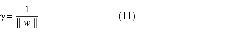
Equation (11) gives us a simple set of parameters to learn in order to maximise the margin for a linear SVM. Given that any new training data points must be classified as greater than 1 or less than −1 the following constrained optimisation problem can be found:
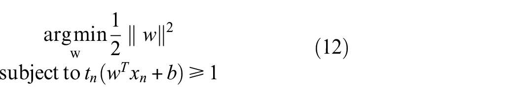
The clear issue with basic SVMs is the identification of a suitable set of support vectors when the training data overlaps, which can lead to violation of the constraint condition in Equation (12). In addition, where a ‘hard’ margin is enforced (which means no data is allowed to overlap the decision boundary), the SVM can be vulnerable to overfitting to a few support vectors. This is avoided by applying a ‘soft’ margin, which allows for an error term for each support vector. This term quantifies the distance between the margin and the support vector for n support vectors, allowing them to sit within the margin or on the wrong side of the decision boundary. This error term is included in the constraint equation for maximising the margin, as shown in Equation (13).

The contribution of the error term for each support vector to the optimisation function is controlled by the multiplier C, which forms a key hyperparameter when training SVMs. The new constraint equation for linear SVMs with soft margins is given as follows:
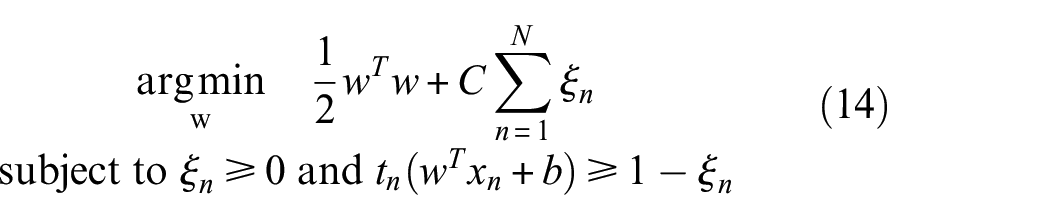
SVMs can be trained using model predictions for FMD-SHM. The ability to generate labelled predictions of the features from anywhere in the damage space is a major advantage of FMD-SHM and can be used to tailor learning process for the classifier (subject to the model predictions offering an adequate fit to real experimental data). As an example of how classifiers can be tailored to data, for the damage detection case it may be reasonable to assume that the normal condition data can be approximated by a Gaussian distribution. This assumption can be tested using stochastic model predictions of the undamaged case, with fit to a Gaussian distribution assessed using an appropriate metric (such as Kullback–Liebler divergence). If the Gaussian assumption on normal state data can thus be satisfied, it would be reasonable to adopt an RBF (alternatively referred to as a ‘Gaussian’) kernel to distinguish damaged and undamaged state data at the detection stage. In all cases, cross-validation is required to set the hyperparameters of the classifier. This allows for an optimised classifier to be trained and also gives an indication of the expected performance of the classifier when exposed to new data.
The global damage detector for the bridge was constructed by training local SVM damage detectors for each strut. The four SVMs were then exposed to the test data, and the classification scores were summed to derive a global classification score. This was then compared to a decision boundary in order to label to the test data as either healthy or damaged. The SVMs were trained and optimised using cross-validation minimisation to select the optimal kernel, kernel scale and C value for each SVM. The training data generated using the physics-based models in this study matched the test points from the assembly-level damage testing described earlier in this paper. This entailed predictions of the bridge in its healthy condition and with damage introduced to struts 1, 5, 2 and 6 (Figure 9), where damage was introduced to the midpoint of each strut in increments of 2.5 mm up to a maximum extent of 17.5 mm. For each damage case, the posterior predictions were evaluated for each damage model. The struts used in this dataset – 1, 5, 2 and 6 – represent the four structurally ‘unique’ struts in the assembly, as the bridge can be divided into four symmetrically identical quadrants along the
In order to evaluate the success of the FMD-SHM method on this dataset, two data-driven methods were developed for comparison. The first of these was a novelty detector, which used a one-class SVM for each strut. These SVMs used an RBF kernel and C value of 1 by default. The training data for the novelty detector was drawn from the assembly-level dataset, utilising the undamaged-state data points drawn from the damage-state testing and boundary condition testing. The data was therefore not dependent on damage-state data from the assembly, but would be limited to the damage detection task only, whereas the model-based strategy could feasibly be extended to other SHM tasks. The detector relied on the physics-based model for feature selection. Setting of the decision boundary would also be very difficult in industrial applications if models or assembly-level test data were not available.
A supervised data-driven damage detector was also trained using the damage-state test data. The SVMs were trained on the same dataset as the novelty detector, with the addition of the damage-state data at the extents of 5, 10 and 15 mm. These SVMs were optimised similarly to those used for the FMD-SHM method. This detector was clearly dependent on assembly-level data across damage states – a major drawback for many SHM strategies. For both the novelty detector and the supervised damage detector the individual strut SVMs were combined to create a global damage detector in the same way as the FMD-SHM damage detector.
Results
Classifiers are generally assessed on their performance in terms of accuracy metrics such as sensitivity and specificity. Features such as these aim to capture the ability of the classifier to correctly label datapoints as being from the class that they are drawn from in reality. The TPR and FPR for classification are dependent on the classification threshold, where increasing the threshold will increase the rate of true positive labels, but simultaneously increase the FPR. A good classifier will maximise the ratio between the TPR and the FPR, and the setting of the classification threshold is clearly key to this.
One way to rigorously evaluate the performance of a classifier is through the receiver operating characteristic (ROC); this covers the TPR and the FPR over a range of classification thresholds. The ROC curves are plotted for the classifiers generated in this paper in Figure 22. The damage thresholds indicated for each subfigure define any crack of depth equal to or greater than the threshold as damaged.
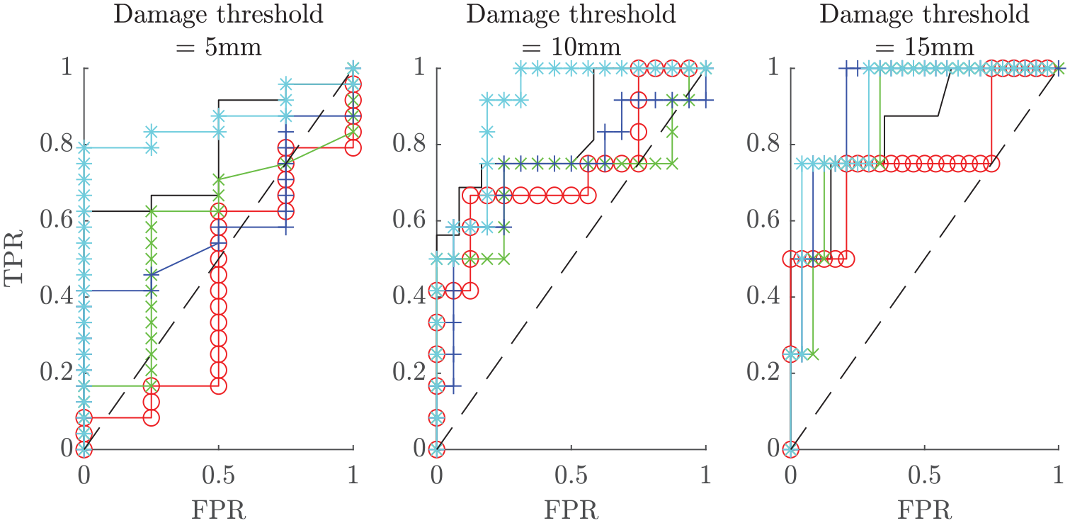
ROC curves for the novelty detector (black), supervised detector (red), model 1 detector (green), model 2 detector (blue), model 3 detector (cyan) with the boundary for informative classification marked with a dashed line.
The area under the ROC curve gives a useful scalar metric for a classifier, where the minimum value for an informative classifier would be 0.5. These values are plotted against damage threshold for the classifiers in Figure 23.
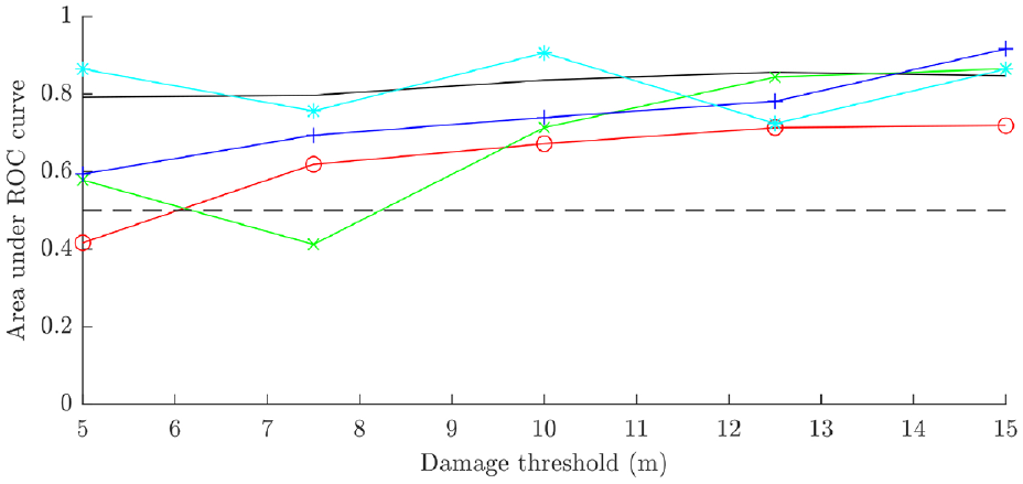
The area under the ROC curves at a range of different damage thresholds for the novelty detector (black), supervised detector (red), model 1 detector (green), model 2 detector (blue), model 3 detector (cyan) with the boundary for informative classification marked with a dashed line.
The initial conclusions that can be drawn from Figures 22 and 23 are promising: the FMD-SHM detectors performed reasonably well compared to the data-driven methods. However, it is possible that the FMD-SHM detectors could be further improved by selecting an updated feature set using the validated models. The initial feature set was selected using the unvalidated, nominal condition models; given the increased accuracy and knowledge of the uncertainty in the model predictions following validation, a more informative feature set may be found that would improve these results further.
Two new feature sets were selected using the validated models to investigate this hypothesis. Feature set 1 – the original set used – was selected prior to validation. The matched features were selected based on damage sensitivity and the MAC. The features were ordered in terms of damage sensitivity (the proportional change in natural frequency at the greatest damage extent) and the less sensitive half of the set was discarded. The two features that maximised the MAC between the model predictions and experimental data within the remaining features were selected. This process was repeated using the validated models for feature set 2. ‘Minimum sensitivity’ was used as a measure of damage sensitivity; this was the proportional change in natural frequency at the greatest damage extent for the posterior sample that showed the least sensitivity to damage. Using the minimum sensitivity was intended to value robustness in the damage sensitivity of the features. For feature set 3, damage sensitivity was prioritised over the MAC, where the two features selected from the matched mode set were simply the ones that showed the greatest minimum sensitivity.
The classification results for the three feature sets are plotted in Figure 24. It can be seen that the reselected feature sets 2 and 3 offer a slight improvement in classification performance for models 1 and 2. This was not the case for model 3, with the reselected feature sets proving less useful than the original features selected prior to validation. This is not necessarily very surprising given the strong performance of the original feature set. It is noticeable that the classification results are relatively robust to feature selection, which offers some credibility to the overall model performance, as good accuracy can clearly be obtained for a large range of predictions.
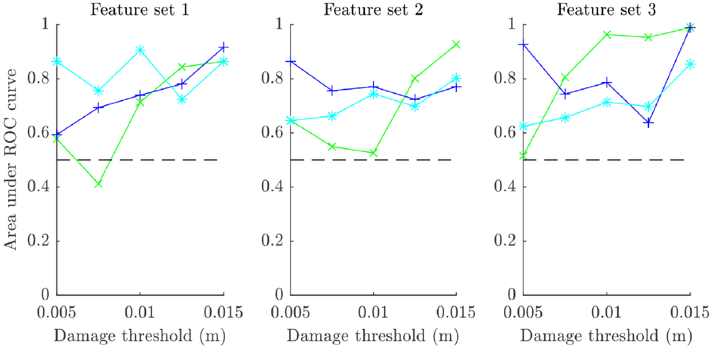
The area under the ROC curves at a range of different damage thresholds for the novelty detector (black), supervised detector (red), model 1 detector (green), model 2 detector (blue), model 3 detector (cyan) using three features sets.
Concluding remarks on damage detection task
The results of the damage detection task for this case study are very pleasing. The FMD-SHM method proved successful using the training data from the hierarchically validated models and performed very favourably when compared to traditional data-driven methods.
The data-driven methods were reliant on the model themselves, which was utilised to select the features on which they were trained. Furthermore, while the novelty detector performed particularly well, it should be noted that it would be very difficult to set an optimal classification boundary without further utilising the models.
The good performance of the FMD-SHM method was particularly pleasing given that it was achieved – through hierarchical validation – without the use of any damage-state assembly data (this was required for the supervised learning data-driven model). Further credibility for hierarchical validation can be drawn from the fact that the best-performing damage model for the classification task was model 3; this was identified at the strut level as the most accurate of the three models (followed by model 2 and finally model 1 – this prediction also proved to be to correspond to assembly-level classification performance).
The features selected prior to validation proved to be useful for damage detection after validation, which backs up the hypothesis that models can be used in a relatively coarse form for the feature selection task in SHM. Fresh features could be selected using the models after validation – these new feature sets improved the performance of classifiers trained using model 1 and model 2.
A further application of the validated models in classifier design would be to set an optimal classification threshold. Given the demonstrable accuracy of the models based on the hierarchical validation process, this could again be carried out without the requirement for any assembly-level damage-state data. Instead, cross-validation of the model predictions could be used to determine an ideal classification boundary with confidence. This could be carried out based on a risk-based framework to design a suitable cost function using classification metrics such as the TPR and the FPR.
Additional extensions of the work presented here would be to use the stochastic predictions to train a probabilistic damage detector; this would be more informative in a risk-based context as mentioned above.
Damage assessment
Damage assessment refers to the task of determining the severity of a class of damage. Assessment can be carried out as a classification task, where damage is assigned some discrete severity label, or by regression, where the severity is assigned a value from a continuous distribution.
Rytter’s hierarchy progresses from damage detection to localisation prior to assessment. 2 Localisation and categorisation of damage is generally required before the severity of damage can be determined for a particular type of damage. The work presented in this paper relied on the use of natural frequencies as features; due to their global nature this presents significant difficulties when carrying out damage localisation. Localisation is particularly difficult for the truss bridge due to the lines of symmetry in the structure and the number of natural frequencies very close to each other in the frequency spectrum. Therefore, the study of damage assessment in this paper is carried out based on the assumption that the location and type of damage is known.
Damage assessment methodology
The validated models were tested on their ability to train a regression model to assign a value to the depth of a crack at the midpoint of each strut of the bridge. This was based on the assumption that the strut containing the crack and the location of the crack was known, and that the damage was known to be an open edge crack.
The regression model selected for this task was the Gaussian process (GP). GP function on the assumption that the underlying distribution of a system can be represented by a collection of normally distributed processes. They are highly flexible and, given sufficient training data, can be fitted to any given underlying function – this is dependent on the mean and covariance functions of the GP, which operate similarly to the kernel for other machine learning algorithms. A key advantage of GPs is that they contain an inherent uncertainty estimation alongside their mean prediction for a given input; this allows for confidence to be attached to any models used for damage assessment. For a detailed explanation of the mathematical basis for GPs, the reader is referred to Rasmussen and Williams. 36
The GP regression models trained for this chapter were fitted via the MATLAB function ‘fitrgp’ using quasi-Newton optimisation. Bayesian optimisation was used to select the covariance function and the hyperparameters. The training data were assumed to contain measurement noise.
The training data used for the damage assessment task were the same as those used for the detection task. The label set was expanded in the training data for this task; instead of the labels being damaged or healthy, as was the case for training damage detectors, the labels were the damage extents at which the training data were generated. Each of the three feature sets used for damage detection were applied to this task. This constitutes an expansion in the dimensionality of the learning space, but with no additional training data provided compared to the damage detection task. As such, a lower level of accuracy should be expected compared to the damage detection results (this is in addition to the fact that damage assessment is inherently a more challenging task for statistical models).
Results
The results of the GP regression models are plotted in Figure 25, which shows the predicted crack depths based on the feature inputs derived from the experimental data (the same test data that was used for the damage detection task). All three damage models were tested on each strut, as were all three feature sets.
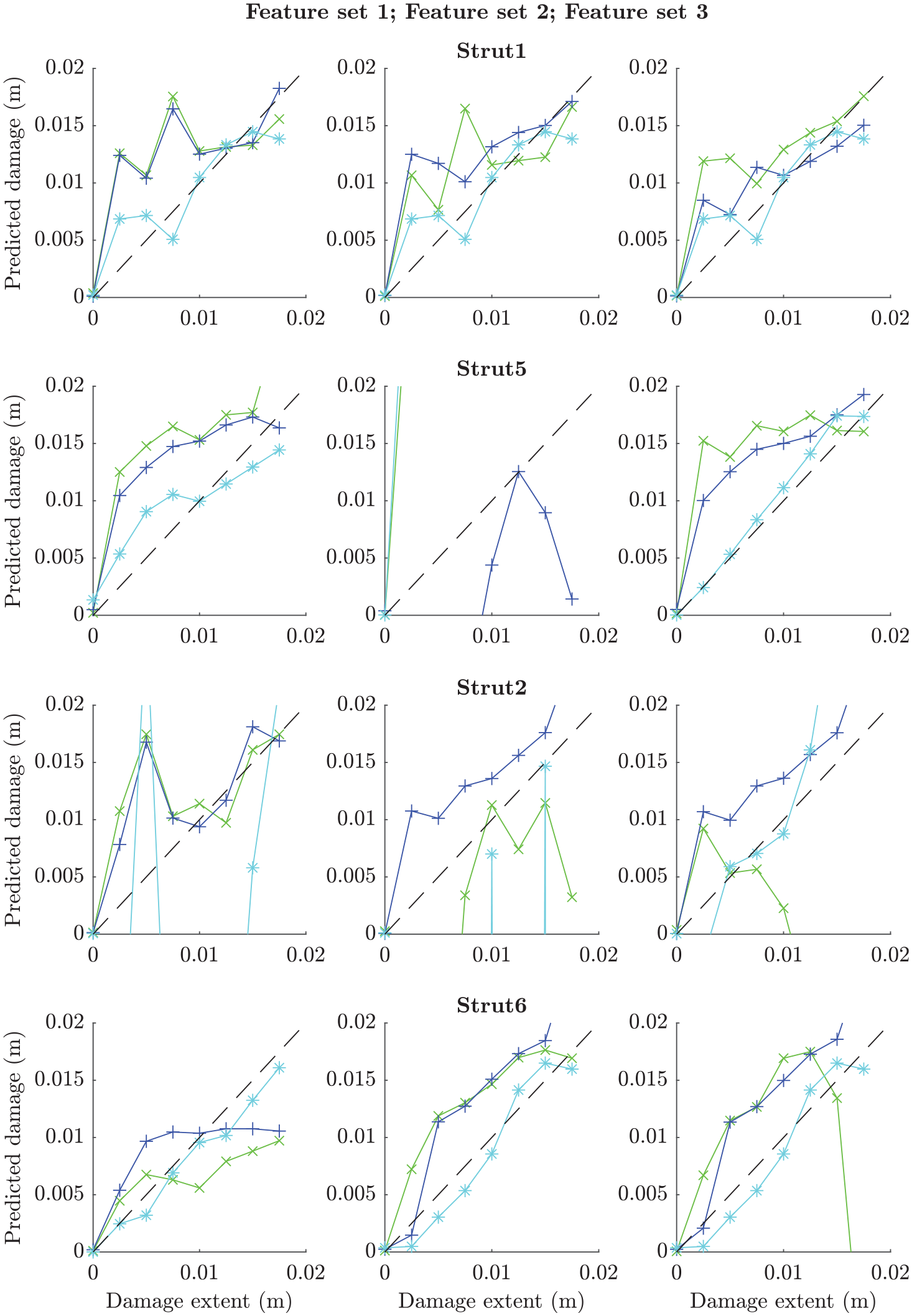
The predicted damage extent compared to the true value for model 1 (green), model 2 (blue) and model 3 (cyan) with the ideal regression model marked as a dashed line.
It can be seen from Figure 25 that the success of the FMD-SHM method for damage assessment is mixed. The rate of damage progression is well-captured by the statistical models in some cases, such as for Strut 1, but for others the accuracy of the regression models is poor. In a number of cases, the predicted damage extents are not physically possible (the predicted crack depth being either less than zero or greater than the depth of the strut). Model 3 appears to be the most robustly accurate across the test data, and it is also apparent that the models are able to more accurately predict crack depth at greater damage extents. It is difficult to judge which of the models performs the most accurately for the damage assessment task, as the variability in accuracy is very significant from case to case.
Concluding remarks on damage assessment task
The damage assessment task was attempted using FMD-SHM techniques based on the three validated damage models. GP regression models were trained using the model-generated datasets and were successful in predicting the depth of cracks in the struts – given knowledge of the damage location – for most cases. Poor predictive performance, such as the model 3 regression model for damage in strut 2 based on feature set 1, can be linked to poor feature matching and selection; Figure 21 shows that the damage sensitivity in this feature space was low, and the model predictions do not correlate well with the experimental data for feature 2. This indicates that the poor performance of certain sets of predictions are due to inadequate feature matching and selection, although model discrepancy could also cause inaccuracies in these cases.
Most of the results show that accurate prediction of damage extent is difficult when the crack length is small, but accuracy is much better at greater damage extents. This is to be expected, given that examination of the selected features has shown that lesser damage extents have relatively small impact on the natural frequencies, whereas much greater sensitivity was observed at greater damage extents (see Figures 19–21). This makes the data at low damage extents very sensitive to noise, and the stochastic model predictions have significant overlap, making separability of the data difficult, which in turn makes it difficult to confidently assign a particular estimate of crack depth.
There is scope for the GP models to be significantly improved by developing a more advanced probabilistic set of beliefs. It is known that the predicted outputs of the models cannot physically be less than zero or greater than 20 mm; this could therefore be incorporated into the model prior to improve the hyperparameter learning process.
Further improvements to this investigation could also be likely made with more precisely targeted experimental data; if a test was focused on a single strut, then the test data could be recorded with more sensor locations to allow for more accurate feature matching. This would allow for more confidence to be attributed to the model predictions, and it would be easier to determine the true sources of error in the model predictions (these could be due to model discrepancies or to mismatching of features). Similarly, generating more training data at a larger range of damage inputs would be expected to improve the performance of the trained statistical regression models.
Discussion and evaluation
A novel application of hierarchical V&V for FMD-SHM was presented in this paper. The ideas were tested in a damage detection and assessment scenario and were shown to perform well compared to data-driven methods. In addition to these results, there is scope for further exploitation of model-based SHM methods which are discussed in this section.
A key benefit of the model-based approach is that the performance of a proposed SHM system can be evaluated prior to any experimental data becoming available; as experimental data becomes available this evaluation can be further refined. This was demonstrated by the selection of the feature space based on validated model predictions prior to the incorporation of experimental damage-state data. While this study used a fairly small set of candidate features (the first few natural frequencies of the structure), this could potentially be significantly extended when applied to a more extensive project, allowing for the selection of a more highly informative feature space.
There is a trade-off to be made between sensitivity and specificity in classifier systems; this is usually based on the setting of the acceptable damage threshold in the context of a damage detection exercise, as was the case in this paper. The setting of the threshold is heavily dependent on the context of the work, and was therefore fairly arbitrary in an academic study such as this. However, in an industry application, the setting of this value should be based on some sort of informed risk analysis; as with the feature selection task, with FMD-SHM methods it is – uniquely – possible to carry out this optimisation task prior to implementation of the SHM system based on the predictions of the physics-based model.
The data required to carry out these pre-implementation optimisation tasks essentially comprises the model evaluations and the subassembly validation data. The latter dataset here allows for the quantification of uncertainty in the model predictions, which allows confidence to be established in the optimisation task. The full set of work upon generating the validated assembly-level model would essentially comprise the following:
1. Selecting a classifier (or a ‘classification structure’ comprised of several classifiers).
2. Defining a cost function based on safety and risk analysis.
3. Selecting an optimisation technique to minimise the cost function defined above.
This process may be computationally demanding. This can be alleviated in a number of ways, the foremost among which would be the use of fast-running surrogates; surrogate models are reasonably well-developed in a structural dynamics context.
Sensor placement is another key issue that limits the successful implementation of SHM strategies; FMD-SHM and hierarchical V&V are no different. A key limitation of the experimental data recorded for this study was the lack of resolution in the mode shapes, particularly at key structural locations such as the struts. The optimisation process enabled by the model can also cover the design of experiments for the SHM system. This would then enable highly effective feature matching and maximise the potential for an informative classifier.
Further work
The FMD-SHM method is applicable across all levels of Rytter’s hierarchy 2 ; due to the exploratory nature of this paper only damage detection and assessment were investigated; however, extensions to localisation and prognosis are key to the further development of the method. Each of these tasks would require more extensive datasets than were required for this study but should otherwise be applicable in a similar style of case study. In addition, the use of validated model predictions to set the decision criteria for the statistical models in FMD-SHM, as discussed in this section, would be a natural continuation from the research presented in this paper.
The quantification of uncertainty in the assembly process is an outstanding issue in the hierarchical V&V process – this problem will require attention in further research concerning hierarchical V&V for SHM. The modelling of joints is closely related to this issue. Joints were neglected from this study, but are known to have contributed to dynamic effects in assemblies. An investigation into the modelling of joints in assemblies, as well as tests of more advanced dynamic substructuring techniques (such as the use of non-rigid connections between substructures), in a hierarchical V&V context would yield further information as to the level of accuracy and confidence that can be achieved through hierarchical V&V.
The application of hierarchical V&V to population-based SHM is an intriguing prospect. Given that structures in a population would be expected to share many components, the individual validation of submodels of these components across the range of damage and operational conditions could be very effective, as the submodels could then be integrated into a large range of nominally similarly assembly-level models representing structures across the population. Demonstrations of this could be carried out using similar examples to the bridge structure used in this study by applying the validated strut models to different configurations of the assembly.
Finally, an additional problem in the implementation of SHM strategies in industry is the influence of confounding variables which are difficult to separate in the data from the effects of damage. In theory, FMD-SHM is a good method to use in tackling this issue, as physics-based models can be used to generate a wide range of training data across EOVs relatively cheaply, through the use of surrogate models if necessary. Alternatively, validated models would be very useful in identifying features that are robust to the effects of EOVs. 14 However, in either of these applications, it is clear that this would require model validation across these EOVs. A study to investigate the application of a hierarchical V&V strategy in the presence of EOVs would be a significant contribution to the field.
Conclusion
This paper introduced and evaluated the application of a novel framework for SHM incorporating a forward model-driven technique and hierarchical V&V. The aim of this was to demonstrate that the lack-of-data problem that afflicts many data-driven SHM strategies can be mitigated by using simulated data, and that – furthermore – the simulated data could be generated using validated models where the validation data could be drawn from the subassembly level. This was carried out and demonstrated through a case study, showing that the dependence on assembly-level damage data for SHM systems (which is often extremely expensive to acquire) could be avoided entirely.
While the results of the SHM systems trained in this paper are not comparable in terms of accuracy to the state of the art in other methods, and the testing dataset was somewhat limited, the results shown in the paper are highly encouraging as the methods presented performed well compared to supervised and unsupervised data-driven techniques on the same dataset. This has significant potential impact in the field, since no assembly-level damage state data were required in developing these methods. Further to this, there are clear next steps to be taken which could be expected to refine the process followed in this paper, and to expand the scope to further SHM tasks.
Footnotes
Declaration of conflicting interests
The authors declared no potential conflicts of interest with respect to the research, authorship, and/or publication of this article.
Funding
The authors disclosed receipt of the following financial support for the research, authorship, and/or publication of this article: This research made use of The Laboratory for Verification and Validation (LVV) which was funded by the EPSRC (Grant numbers EP/R006768/1 and EP/N010884/1), the European Regional Development Fund (ERDF) and the University of Sheffield.