
Abstract
There are a large number of time domain, frequency domain and time-frequency signal processing methods available for univariate feature extraction. However, there is no consensus in SHM on which feature, or feature sets, are best suited for the identification, localisation and prognosis of damage. This paper attempts to address this problem by providing a comprehensive benchmark of feature selection & reduction methods applied to an extensive set of univariate features. These univariate features are extracted using multiple statistical, temporal and spectral methods from the benchmark S101 and Z24 bridge datasets. These datasets contain labelled accelerometer recordings from full scale bridges as they are progressively subjected to multiple damage scenarios. To identify the minimal set of features that best distinguishes between the multiple damage states, a supervised machine learning approach is used in combination with multiple feature selection methods. The ability of these reduced feature sets to distinguish between damage states is benchmarked using the prediction performance of the classification models, with the training and test sets obtained through stratified k-fold cross validation. The results obtained show that reduced sets of univariate features, extracted from a single accelerometer sensor, are capable of accurately distinguishing between multiple classes of healthy and damaged states. This work provides a benchmark for SHM practitioners and researchers alike for the choice, comparison and validation of feature extraction and feature selection methods across a wide range of systems.
Keywords
Introduction
Vibration based bridge SHM involves the installation of sensors that measure the dynamic response of a structure. The dynamic response of a structure is governed by a large number of parameters, such as geometric (e.g. for a bridge: span, deck width, boundary conditions), 1 material (e.g. mass, stiffness, damping), 2 environmental (e.g. temperature, wind) 3 and operational (e.g. live load) 4 factors. Differences in these parameters and the age of a structure influence the SHM methodology and approach and present a significant challenge in the establishment of a standard SHM method for all structures.
Data driven methods for Structural Health Monitoring (SHM) have been established using statistical and machine learning for feature modelling and damage identification.5–8 Due to the dimensionality of high-frequency acceleration data, the selection of features to be extracted from the raw time domain signal is central to this approach. There is still a lack of consensus on the optimal feature, or combination of features, for distinguishing between various damage types. Despite the significant effort applied in the field to establishing the optimal combination of damage sensitive feature and statistical learning model, the performance of each feature and model combination differ based on the assessment scenario and the performance criteria chosen, even for the same structural dataset.9–12
An alternative thought process is to shift from trying to obtain the best method, to establishing a robust framework for distinguishing admissible, good enough methods from inadmissible ones and creating a robust benchmark of damage sensitive features. This framework must account for the significant instrumentation, transmission and storage constraints present when implementing a monitoring campaign on full scale operational structures. 13
Distinguishing the admissible set from the inadmissible will help decide on instrumentation monitoring, data interpretation, comparison and consistent decisions based on data, leading to increased value of information from SHM.14,15
This paper presents a comprehensive analysis of various time domain and time-frequency domain feature extraction methods. The ability of these features to distinguish between multiple damage states is evaluated using supervised machine learning models. Additionally, several feature selection methods are coupled with these classification models to evaluate whether reduced sets of features can achieve similar classification performance. The goal of this work is to identify the minimal set of features which maximise the ability of a statistical learning model to detect and distinguish between damage in structural systems.
As only a small number of accelerometers are required to capture the global dynamics of a structure, these sensors are extensively deployed for SHM.16–18 However, a key barrier to the full deployment of remote continuous SHM systems is energy-hungry transmission19,20 and storage requirements 1 of acceleration data. In order to capture the full range of dynamic response, a sampling frequency between 100 Hz to 500 Hz is generally used. 21 The data gathered from accelerometers during a SHM campaign quickly presents a ‘big data’ challenge. The dimensionality of the data due to this high sampling rate presents a significant challenge in transmitting and modelling the data. Pre-processing, feature extraction and dimensionality reduction techniques are therefore applied to the recorded raw acceleration data before modelling and statistical inference can be implemented.
Low power data transmission technologies such as LoRa 22 are extremely limited in the size of the data packets that can be transmitted per hour. Therefore, for accelerometer sensors system, data compression or feature extraction at the edge is required so that low data sized representations of the signal can be streamed offsite for modelling and analysis.23,24 The initial choice of features is of particular importance in the context of a wireless sensor network as feature extraction methods need to be pre-configured and pre-coded onto edge devices before deployment. 25
Feature extraction methods are employed to obtain useful lower dimension metrics from the raw time domain signals. The features extracted from acceleration signals are calculated over a set time window and provide a summary of the dynamic characteristics of the structure over that window. The change in these features over time are indicative of the behaviour of the dynamical system under measurement. In the context of remote monitoring, feature extraction methods are categorised in this work as either univariate, obtained from the raw measurements of a single sensor, or multivariate, obtained from the raw measurements of multiple sensors.
Multivariate parametric features capture dynamic characteristics of the structure, specifically natural frequencies, damping ratios and mode shapes. These features require inputting the raw acceleration data from each sensor into a large matrix. The streaming of the raw acceleration data offsite is not possible in a low power wide area network. Even if low power data transmissibility is not an issue due to consistent power supply for each sensor system, damage localisation is not possible when analysing features obtained using multivariate feature extraction methods and the raw acceleration signals cause additional challenges and costs in transmission latency and data storage and processing.
Univariate features are extracted from the raw acceleration data of an individual accelerometer. This enables feature extraction at the edge and the wireless transmission of lower dimensional features for analysis. Another advantage of univariate feature extraction is the potential for damage localisation by comparing features sampled at the same time point from different sensors located across the structure. However, univariate features have received less attention in the SHM literature. Unlike multivariate methods, univariate feature extraction loses the ability to carry out system identification and identify global structural characteristics such as mode shapes or the global natural frequency of the structure. As univariate features are not based on structural parameters, it is difficult to determine how much variation in the signal statistics is due to variations in environmental and operational effects or due to the occurrence of damage. The univariate features that can be extracted from a single acceleration signal can be categorised as statistical time domain features, temporal time domain features and spectral time-frequency domain features.
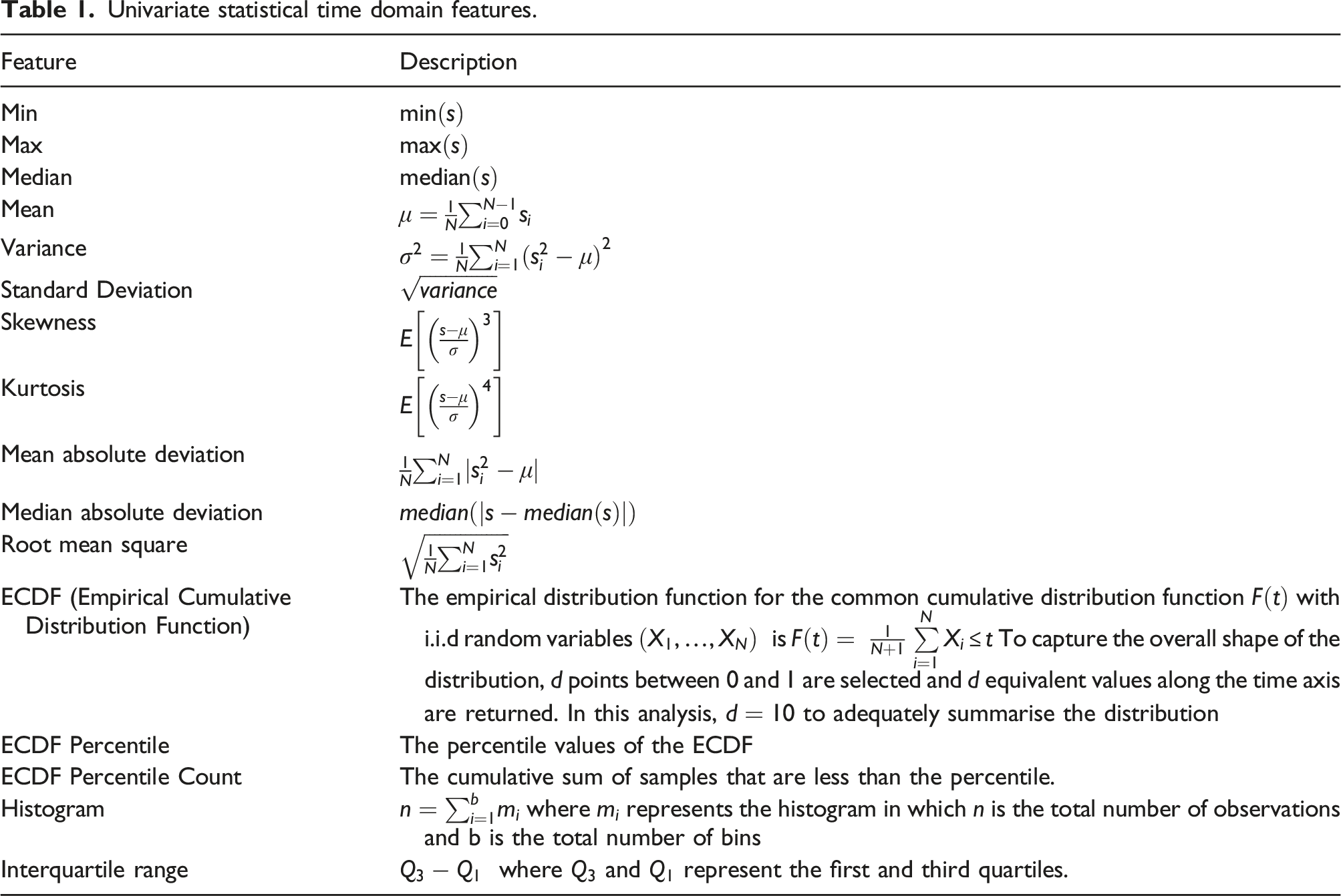
Statistical features are the simplest features computationally that can be extracted from a signal. These features are computed in the time domain and provide a summary of the statistics of the signal over the feature extraction window. Some of the primary statistical time domain features used include mean, variance, standard deviation, skewness, kurtosis, Root Mean Square (RMS)26–28 and the difference in empirical cumulative distribution functions. 29 Statistical features such as RMS have also been used in combination with modal parameters as Damage Sensitive Features (DSFs).30–32 The advantage of statistical features is the simplicity of their computation which becomes particularly important for edge feature extraction on microcontrollers in a wireless sensor network. 33
Temporal features provide information about the dynamics of the signal over time. Energy-based temporal features have been examined in [34] in relation to damage detection in the S101 bridge. One of the most prominent temporal features used in the SHM literature are the coefficients of a univariate autoregressive (AR) model29,35–37 or variations including auto-regressive moving average (ARMA) 6 autoregressive model with exogeneous inputs.38,39 Although an effective method for damage detection in experimental structures, AR models have had little success in full scale applications; they are incapable of representing nonlinearities and assume that the time series is stationary. 6
Spectral or time-frequency features represent the behaviour of the data in the frequency domain over time. Some of the primary spectral methods include short-term Fourier transforms (STFT), cepstrum coefficients, wavelet transforms and mode decomposition methods. Mode decomposition methods decompose the signal into intrinsic mode functions (IMFs). The Empirical mode decomposition (EMD) is the first step in the Hilbert Huang Transform (HHT) used to obtain instantaneous frequency data.40–42 Ensemble EMD (EEMD) is a popular method to prevent mode mixing problem. 43
STFT involves the calculation of the Fourier transform for windows of the data, with the changing spectra obtained by shifting the window through the entire time series signal. The changing spectrum of frequencies over time produces a spectrogram whose coefficients at each frequency can be used as DSFs.44,45 From either the magnitude or the power (squared amplitude of the STFT) features describing the statistical properties of the signal and the magnitude of the spectrum can also be computed.46,47
The use of cepstrum/cepstral coefficients as damage sensitive features has received a renewed focus in SHM over the last number of years.37,47–49 The Cepstrum is the inverse Fourier transform of the logarithm of the Fourier spectra magnitude squared. 50 Cepstrum analysis has shown promise as an efficient measure for detecting changes in a signal that are not easily identified in the spectrum. 47 In Ref. [37], the link between cepstrum based features and modal properties of a structure are defined with cepstrum features found to be an effective measure of damage detection.
The STFT is limited in that the fixed-length window leads to a fixed time-frequency resolution across the whole time-frequency domain. To optimise the time-frequency resolution for diverse spectral components in a signal, the window size should be varied. A continuous Wavelet Transform (CWT) addresses the fixed time-frequency resolution of the STFT by using adaptive variable time windows that are short in the high-frequency range and long in the low-frequency range. These windows are achieved through the use of wavelet functions.51,52 Wavelet transforms are one of the most well studied spectral feature extraction methods used in SHM.44,53,54 Wavelet transforms have also shown significantly higher accuracy in noise inference than the Hilbert Huang Transform. 41
Modal parameters can be identified in a univariate manner using wavelet based adaptive filtering. 55 Locally decentralised procedures using wavelet clustered filter banks for real time identification of modal parameters and localised damage detection have been developed with a view towards wireless sensor nodes.56,57
There are numerous features and feature types available for SHM. There is no universal agreement about the optimum features for different tasks, different structures and different damage types. Each feature type may have varying sensitivity to different forms of damage or be prone to false positives due to environmental and operational effects. A feature library is desirable for more effective SHM analysis by following a feature selection process.58,59
Rather than choosing a single method for feature extraction, the modelling of a combination of features could improve the overall damage detection with some features being more sensitive to particular damage types. However, if condensing and comparing multiple feature sets. It is necessary to characterise the statistical significance of features used. 60 Therefore, feature selection methods applied to multi-class datasets, where the classes in this scenario represent different damage states, are required to assess the significance of feature types and feature combinations on their ability to distinguish between damage states. Time-domain, frequency-domain and time–frequency domain features can be integrated to express the information in a signal more comprehensively. This approach has been extensively applied in the domain of bearing fault diagnosis,61–64 but it has yet to be applied to SHM datasets with multiple damage states. 59
Feature selection methods require a supervised learning approach where knowledge of the varying damage states or classes is available in order to identify the subset of informative features that best discriminate different classes. Once an optimal feature subset is identified, this could then be used as the input to unsupervised novelty detection algorithms for real-time damage detection. Most datasets contain irrelevant, highly correlated or noisy features that can be removed without a significant loss in information. Feature selection has become fundamental for data analysis, machine learning and data mining applied to high-dimensional datasets. 65 Feature Selection methods can be placed in three categories, filter methods, wrapper methods and embedded feature importance methods. Filter feature selection methods calculate the relevance of each feature with respect to the target classes. The features can then be sorted based on their individual relevance to the classes and a top percentage chosen for modelling. 66 Filter methods are independent of classifiers and applied before any modelling is undertaken. Examples of filter methods include analysis of variance (ANOVA), maximally relevant and minimally redundant (MRMR) and minimisation of joint mutual information (JMI). A comparison of filter methods for high-dimensional data from different fields is provided in Ref. [67]. Wrapper feature selection methods are greedy search algorithms that optimise model performance based on fitting a classification algorithm to different subsets of input features. The best feature set is the one which maximises the classification prediction accuracy. Recursive Feature Elimination (RFE) is an efficient backward selection algorithm that uses intrinsic model importance to rank features. Intrinsic or embedded feature importance is a measure of how each feature influences the predictions of a specific classification model. Model importance is embedded as it provides a link between the features and the modelling objective function. The objective function is the statistic being used by the classification algorithm to model the data. A feature subset obtained using RFE coupled with a Random Forest algorithm has been shown to improve classification accuracy on the ASCE benchmark dataset using wavelet packet transform features. 68 A number of filter, wrapper and embedded feature selection approaches have been applied to the binary scenario where two data sets are available from the Tianjin Yonghe Bridge before and after a damage occurrence.27,47,69. Feature selection based on a genetic algorithm (GA) is proposed in Ref. [70]; however, the results from a demanding feature selection phase are only comparable to an AR model for damage detection in a simple laboratory structure.
In this analysis, supervised learning classifiers are trained on univariate statistical time domain, temporal time domain and time-frequency domain features. Multiple feature selection methods are then implemented to identify the minimum feature set with the highest damage prediction capability. The datasets used are the benchmark S101 and Z24 datasets which contain acceleration recordings from measured progressive damage tests on full scale bridges. This analysis is the first application of feature selection to full scale bridge data with multiple damage states and is the most comprehensive comparison of the damage detection capabilities of statistical time domain, temporal time domain and spectral time-frequency domain features in the field of SHM. Artificial progressive damage events are applied to the Z24 38 and S101 18 bridge datasets to mimic how damage may progress in an operational structure.
For each accelerometer statistical time domain, temporal time domain and spectral time-frequency domain features are extracted using the Time Series Feature Extraction Library (TSFEL) in python. 71 Other libraries available for extracting time series feature from high-frequency signals include TsFresh72,73 and hctsa 74 an empirical comparison of these opensource packages is presented in Ref. [75].
A baseline of univariate damage sensitive features is required for SHM to compare different feature types with a feature selection process to obtain the minimum combination of features with the highest damage prediction performance. This feature subset could then be used as the input to unsupervised learning algorithms to identify damage as it occurs. However, a systematic and organised approach towards such a benchmarking approach has not been attempted to this point.
This paper intends to address this timely requirement in the field of SHM and creates a comparative benchmark for this purpose. Supervised learning classifiers are trained on univariate statistical time domain, temporal time domain and time-frequency domain features. Multiple feature selection methods are then implemented to identify the minimum feature set with the highest damage prediction capability. The datasets used are the benchmark S101 and Z24 bridge datasets, containing acceleration recordings from measured progressive damage tests on full scale bridges. This analysis is the first application of feature selection to full scale bridge data with multiple damage states and is the most comprehensive comparison of the damage detection capabilities.
Methodology
In this section, the theory outlined behind (a) the methods for estimating features from the data, (b) the classification algorithms used to classify these features into different damage states and (c) the selection of minimum feature subsets which maximise classification performance.
Feature Estimation
Univariate features are signal processing methods which can be obtained from individual accelerometer recordings. The features extracted from acceleration signals are calculated over a set time window and provide a summary of the dynamic characteristics of the structure over that window. The change in these features over time is indicative of the behaviour of the dynamical system under measurement. While individual features may have varying sensitivity to different forms of damage or be prone to false positives due to environmental and operational effects, the fusion of features could provide a greater overall damage detection capability and robustness to false positives.
Statistical Time Domain Features
Statistical time domain features are the simplest features computationally that can be extracted from a signal. These features that are computed in the time domain provide a summary of the statistics of the signal over the feature extraction window.
In the following formulae,
Temporal Time Domain Features
Temporal features provide descriptions of the dynamics of the signal over time during the feature extraction window. These features are also extracted from the time series signal. In the below temporal feature equations,
Time-Frequency Domain Features
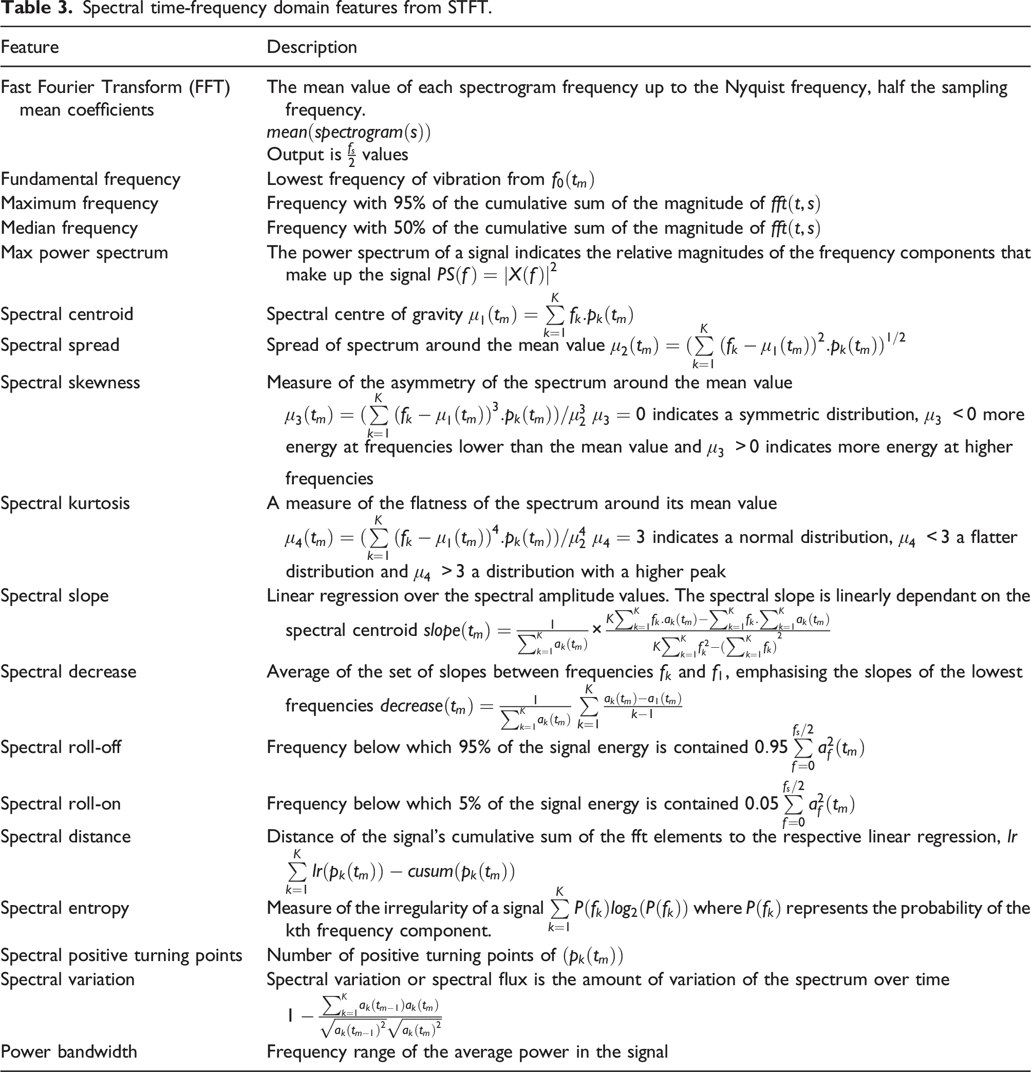
Spectral time-frequency features represent the signal change in the frequency domain over time. Three spectral approaches to obtaining time-frequency domain features are used in this analysis. These are the Short Term Fourier Transform (STFT), Cepstrum Coefficients and Wavelet Transforms.
Short Term Fourier Transform
The first set of spectral features is obtained from the application of a Short Time Fourier Transform (STFT) to the signal window. The Fourier transform is calculated for each block or window of the data, with the changing spectra obtained by shifting the window through the entire time series signal. The changing spectrum of frequencies over time produces a spectrogram with the horizontal axes representing time and the vertical axis representing frequency up to half the sampling frequency
The discrete-time STFT is related to the discrete-time Fourier transform, given by


Univariate statistical time domain features.
Univariate temporal features.

From either, the magnitude or the power (squared amplitude of the STFT) features describing the statistical properties of the signal and the magnitude of the spectrum can be computed. 46
In the following, the frequency and amplitude of the bin 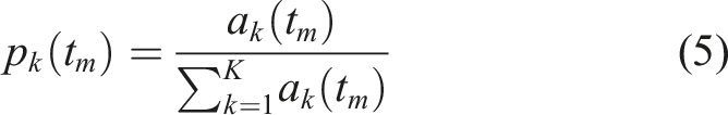
As the data is windowed to obtain discretized signal vectors to input into feature extraction algorithms, this can create spectral leakage when extracting frequency domain features. The signal is non-periodic and the Fourier transform assumes periodicity. Any significant differences in the start and end of the window of data become a sharp step change under that assumption, producing a lot of extra coefficients and noise. Multiplying the data by a window function can help mitigate that problem by reducing the magnitude down to zero or near-zero at the edges of a window.
A Tukey window is chosen over a hanning window as it better captures transient events than a hanning window. The choice of overlap in the windows is a balance between spectral leakage and spectral resolution. As the Tukey window is closer to one for a longer period of time, then the 50% overlap (factor of 2) often used for hanning windows is not required. When computing a spectrogram, or other time-frequency features, a smaller overlap maintains some statistical independence between individual segments of the spectrogram. 77 Therefore, a Tukey window with a 12.5% (factor of 8) overlap is used in this analysis.
Spectral time-frequency domain features from STFT.
Cepstrum Coefficients
The next set of spectral features are in the quefrequency domain known as cepstral or cepstrum coefficients. Cepstrum analysis is used for the detection of periodicity in a frequency spectrum. The use of cepstrum/cepstral coefficients as damage sensitive features has received a renewed focus in SHM over the last number of years.37,47–49 The Cepstrum is the inverse Fourier transform of the logarithm of the Fourier spectra magnitude squared. 50 Cepstrum analysis has shown promise as an efficient measure for detecting changes in a signal that are not easily identified in the spectrum. 79 In Ref. [37], the link between cepstrum based features and modal properties of a structure are defined with cepstrum features found to be an effective measure of damage detection.
The cepstrum of a signal is the inverse Fourier transform of the log-spectrum of that signal. The mel frequency cepstral coefficient (MFCCs) is the most common method of cepstral analysis used for damage detection in structural systems. The MFCC is a compact representation of the logarithm of the spectrum of the signal recorded from the structural system.
The application of the Discrete Fourier Transform (DFT) to each filtered signal window provides the short term power spectrum 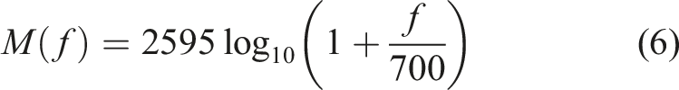
Next, the logarithm of the powers at each of the mel-frequencies is computed. Finally, an L-points discrete cosine transform is applied to the logarithm of the Mel spectra to convert the log mel spectrum back to the time domain. This gives the MFCC features.78,79
The extraction of the MFCCs can be described as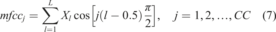
Linear Predictive Cepstrum Coefficients (LPCC) are derived from linear prediction coefficients (LPC). LPC are the coefficients of an auto-regressive model minimising the difference between linear predictions and actual values in a time window. The LPCC can be calculated as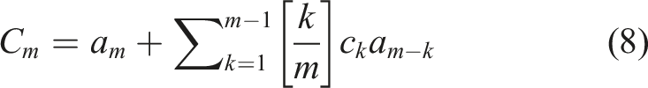
Wavelet Transform
The continuous wavelet transform (CWT) is an effective spectral feature for providing smooth and specific time frequency resolution throughout a signal The STFT is limited in that the fixed-length window leads to a fixed time-frequency resolution across the whole time-frequency domain. To optimise the time-frequency resolution for diverse spectral components in a signal, the window size should be varied. A continuous Wavelet Transform (CWT) addresses the fixed time-frequency resolution of the STFT by using adaptive variable time windows that are short in the high-frequency range and long in the low-frequency range. These windows are achieved through the use of wavelet functions with a Morlet wavelet used in this analysis. 52 Wavelet transforms are one of the most well studied spectral feature extraction methods used in SHM.44,53,54 Wavelet transforms have shown significantly higher accuracy in noise inference than other spectral feature extraction methods such as the Hilbert Huang Transform. 41
The continuous wavelet transform (CWT) is used in this analysis. The CWT of a signal 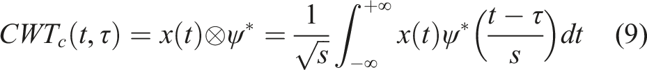


The continuous wavelet transform of the discrete sequence 
The multi-resolution characteristics of the continuous wavelet transform in low and high frequency bands improves the frequency resolution in the STFT, optimising the time-frequency resolution. Like with the STFT, features describing the statistical properties of the signal can be computed from the wavelet transform. These include the mean, absolute mean, variance and standard deviation of the continuous wavelet transform. Temporal features, energy and entropy of the CWT are also included.
Pre-Processing
The scale of features often differ significantly in magnitude. This can be solved by normalising features between a value of 0 and 1. The scaler takes each feature value, 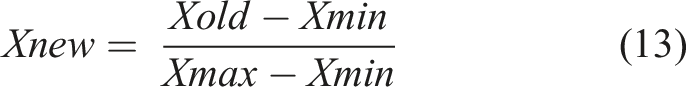
Normalising the features alleviates issues in classification and prediction. Without normalisation, features of a higher magnitude can incorrectly receive higher weighting for distance-based algorithms. Step sizes can also differ based on feature magnitude for models using gradient descent.
Feature Extraction Process
The process for extracting the presented features is shown in Figure 1. Feature extraction process.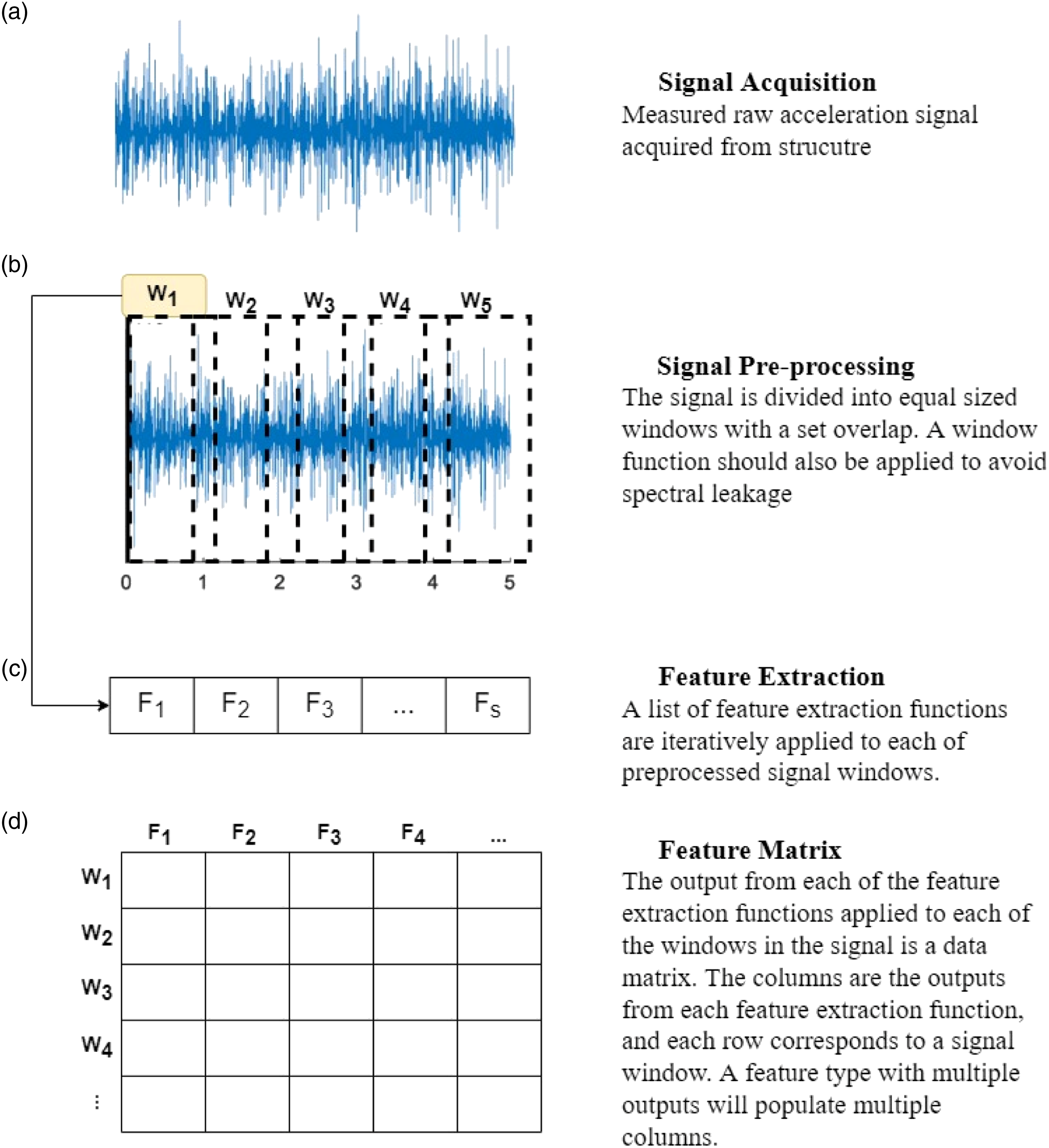
Classification
The first goal of the analysis is to determine whether classification of the different damage states can be performed using the full set of extracted statistical time domain, temporal time domain and spectral time-frequency domain features.
A set of five classification algorithms were chosen for this analysis. These models are chosen based on their use in SHM literature and their interpretability in terms of how they use features to predict output classes. The classification algorithms chosen for this analysis are a Support Vector Machine (SVM), Bagged Tree, Random Forest, k-Nearest Neighbours (kNN) and Naïve Bayes.
Neural network type models are known to be effective in capturing the nonlinear relationship between input features and the target. The issue with a neural network model is its low interpretability as it is very difficult to obtain the influence of each individual feature from a neural network model, particularly for multi-class classification.
Stratified k-fold Cross-Validation
Features are labelled based on the damage state they were extracted from and split into training, validation and test sets. The validation set is necessary to tune model hyperparameters and avoid overfitting of the model on the training set. The classification performance is then measured on the unseen test dataset.
Splitting the dataset into three sections significantly reduces the available data for training the classification models. K-fold cross validation can be used to utilise the full training dataset and provide robust models trained and validated over the entire training dataset. Cross validation splits the training set into K folds. The model is trained using K-1 folds and the last fold used for validation. For the next K-1 iterations, alternate folds are held out. The performance reported by K-fold cross-validation is the average of the values computed over the K iterations. By utilising the entire training set, cross validation also helps against overfitting.
The choice of K folds is based on balancing variance and bias across the dataset. A lower K value results in less variance but more bias, and a higher K value results in more variance but less bias. Overfitting occurs when there is too much variance and underfitting occurs when the bias is too high. Generally, a values of five or 10 are chosen for K. 80
Often in real life datasets, imbalance is present in the distribution of the class sizes. This can result in some folds containing few or no examples from smaller classes. Skew in the distribution of class sizes can also lead to models increasing classification accuracy by attributing values to the larger classes rather than classifying based on actual data values. Stratified K-fold cross validation utilises stratified sampling to ensure that the relative class frequencies are preserved across training and validation folds.
Support Vector Machine
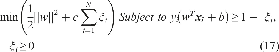
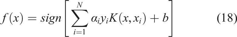
Support Vector machine is a kernel method which constructs a set of hyperplanes in a high dimensional space for classification. It is an effective supervised machine learning method for the classification of damage states.8,41,81,82
Classification is performed in a binary manner by obtaining the maximum margin hyperplane that divides a group of points 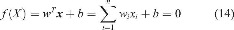
If both classes are completely separable, the data should satisfy the constraints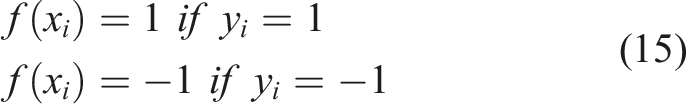

For multi-class classification, the binary SVM algorithm can be implemented in a one versus all or a one versus one approach.
Bagged Tree
The Bagged Tree model is an algorithm which uses bootstrap aggregation ‘Bagging’ in conjunction with a decision tree to construct an ensemble.
Decision trees are ideally suited for ensemble-based methods as they are high-variance, weak classifiers that can be easily randomised. Trees are constructed on a bootstrapped dataset of the original data. Each tree partitions the data in a hierarchical manner with each branch of the decision tree splitting the data based on a mapping from the feature space to the target classes. Splits are made at each node where data samples fall into the right or the left child of the node. Any node in a tree represents a subset of the feature space. Each tree is grown in a two-step procedure for each node. A subset is first chosen at random and then the optimal split is determined by an impurity measure.
Common Impurity measures include variance, Gini index or entropy. 83 Each node splits downward in a recursive manner until a stopping criteria is reached such as a set threshold value. More complex decision trees lead to finer partitions, giving improved performance on the training dataset. To reduce over fitting, regularisation such as maximum tree depth is used to control this complexity.
Each decision tree model in the ensemble is used to generate a prediction of the class for each sample and these predictions are averaged to give the final bagged tree model prediction. The advantage of bagging is that the by averaging multiple noisy unbiased models, the variance is significantly reduced. 66
For the Bagged Tree, the entire feature set is considered when splitting every node in every decision tree, therefore the trees are not completely independent of each other. This tree correlation limits the benefits of averaging and can prevent bagging from optimally reducing the variance of the predictions. 80
Random Forest
The Random Forest algorithm is a modification of the bagged tree which builds a large collection of de-correlated trees before averaging. The idea is that a group of weak and uncorrelated learners is more robust and can generally outperform a single strong learner.
The correlation in trees is reduced by the introduction of randomness in the process of tree construction. For the training of each decision tree in the ensemble, a different random subset of features is chosen at each split in the tree. This results in a diverse ensemble of uncorrelated predictions leading to a substantial reduction in the model variance. Random forests are also more computationally efficient than bagged tree models as the entire feature set is not considered at each node split.
The Random Forest model has had previous SHM applications in predicting natural frequencies, 84 damage detection68,85,86 and crack detection.87,88
k-Nearest Neighbour
k-nearest neighbour (kNN) is an effective nonparametric method for classification which is regularly used in SHM applications.68,89–91 The kNN algorithm computes the distance between each training and test sample in the dataset, returning the k closest samples. The closeness of a datapoint is determined by a distance metric such as the Euclidean distance. The probability of a data point belonging to a particular class is dependent on the proportion of training set neighbours in each class. The primary parameter in the kNN algorithm is the number of neighbours. If the number of neighbours is too low, kNN can be prone to overfitting while too many neighbours lead to boundaries that do not separate the structure of the classes. 66
Naïve Bayes
Naïve Bayes is a classification technique suitable for high dimension feature spaces. Naïve Bayes is a conditional probability model which assigns instance probabilities to each feature in the vector 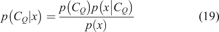
Classification Performance Metrics
The assignment of a datapoint to one of the classes of healthy and damage states is governed by a decision threshold in the range of 0–1. A datapoint is assigned to a class when it is predicted probability for that class is above the threshold. The default threshold for normalised prediction probabilities is 0.5.
Several performance metrics can be used to assess the prediction performance of each classification algorithm. Each metric assesses a different aspect of the classification performance. Some classification models perform better on some criterion over others. 93 The use of a variety of performance metrics is especially important for multi-class datasets as challenges such as class imbalance can cause bias in the classification procedure.
Accuracy Classification Score
Accuracy is the most commonly used performance metric in machine learning.
93
The accuracy score compares the predicted labels, 
Accuracy or error rate applies a Naïve 0.5 threshold to decide between classes. Classification accuracy is based on a count of the errors and does not give any indication about which classes are being confused.
Precision (Specificity)
Precision measures the proportion of true negatives that are correctly identified. Precision is the ratio
Recall (Sensitivity)
Recall measures the proportion of true positives that are correctly identified. Recall is the ratio
Balanced Accuracy Classification Score
The balanced accuracy score is used for imbalanced datasets and is defined as the average recall obtained on each class. This is equivalent to the accuracy score with each sample weighted with weight 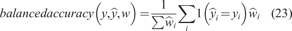
F1 Classification Score
F1 score is a weighted average of the precision and recall. This score can be additionally weighted by support, to account for class imbalance. The F1 score is calculated independently for each class and the weighted based on the number of true instances for each class.
Matthews Correlation Coefficient
The MCC is a correlation coefficient value between −1 and +1 that measures the quality of multiclass classifications. A coefficient of +1 represents a perfect prediction, 0 an average random prediction and −1 an inverse prediction. MCC can be defined in terms of a confusion matrix C for Q classes • • • • 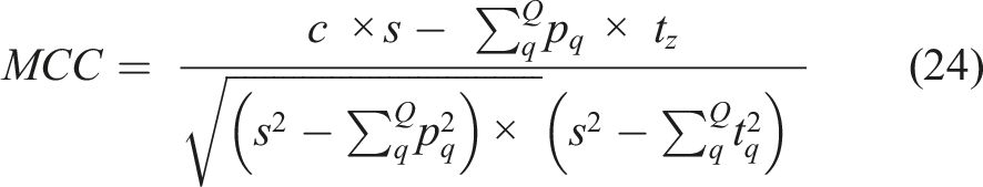
The MCC statistic is also known as the phi coefficient.
ROC-AUC Classification Score
ROC-AUC, or c-statistic, computes the Area Under the Receiver Operating Characteristic Curve (ROC-AUC) from the prediction scores for various classification thresholds. An assumption in the use of classification accuracy as an evaluation metric is that the class distribution among examples is constant and relatively balanced. In the real world, this is rarely the case. The ROC method is a robust, efficient solution to the problem of comparing multiple classifiers in imprecise and changing environments. 94 ROC curves describe the behaviour of a classier without regard to class distribution or error cost, and so decouple classification performance from these factors.
ROC is a probability curve of recall versus 1-specificity, and AUC represents the measure of separability. This metric gives a value between 0 and 1, indicating the capability of the model in distinguishing between classes. For multi-class classification, the AUC of each class can be calculated in a one versus one (OVO) or in a one versus the rest approach (OVR).
Feature Selection
The goal of feature selection is to identify a subset of informative features that best discriminate different classes. Most datasets contain irrelevant, highly correlated or noisy features that can be removed without a significant loss in information. Feature selection has become fundamental for data analysis, machine learning and data mining applied to high-dimensional datasets. 65 For high-dimensional datasets, it is necessary remove non-informative and redundant features to reduce the dimensionality of the dataset, making models easier to interpret. A reduced relevant feature set also decreases the chance of over-fitting by removing noisy features and improves prediction accuracy. 95 The feature subset should provide classification accuracy that is close to the accuracy achieved using the entire feature set. Crucially, for a remote monitoring system, a reduced feature set results in less computation at the edge and less data to transmit. Feature Selection methods can be placed in three categories, filter methods, wrapper methods and embedded feature importance methods.
Filter feature selection methods calculate the relevance of each feature with respect to the target classes. The features can then be sorted based on their individual relevance to the classes and a top percentage chosen for modelling. 66 Filter methods are independent of classifiers and applied before any modelling is undertaken.
ANOVA F-Test
The ANOVA F-test is a filter method appropriate for multiclass classification. The ANOVA, analysis of variance, test is a parametric statistical hypothesis test for determining whether the means of multiple samples are from the same distribution. The F-statistic is then used to calculate the ratio of the explained and unexplained variance from the ANOVA test and rank the features based on their level of variance across the damage states.
The higher the F statistic, the more the mean values of the feature differ between the classes. For each feature 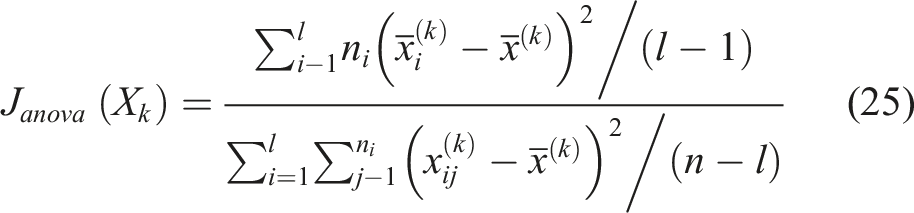
For each of the classification models, we would like to know how the prediction accuracy varies with the inclusion of different percentiles of ANOVA ranked features.
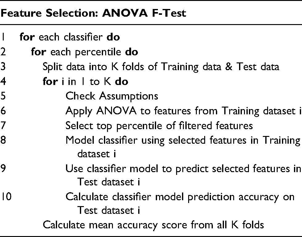
1. To prevent data leakage, the K fold stratified cross validation is first applied to the data.
2. The training set for each feature is checked to determine if the data is normal, has constant variance and is independent and identically distributed.
3. The ANOVA F-Test is then applied to each individual feature based on the training set from each fold.
4. The top Q percentile of features from the ANOVA ranking is selected.
5. The classification algorithm is then applied to the training data and the accuracy of the model predictions on the testing data is calculated.
6. Finally, the mean accuracy from the K cross validation folds is obtained for each classifier.
For the ANOVA test, each feature is evaluated individually, redundant or highly-correlated features may be selected and the combined predictive power of multiple features is not taken into consideration.
Filter methods for feature selection are computationally efficient but the selection criteria of the features are not related to the effectiveness of the classification model.
Wrapper feature selection methods are search algorithms that optimise model performance based on fitting a classification algorithm to different subsets of input features. The best feature set is the one which maximises the classification prediction accuracy.
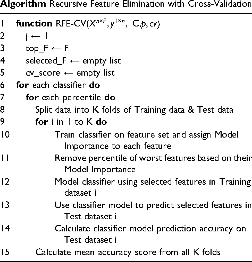
Recursive Feature Elimination
Wrapper methods operate in a sequential manner of feature selection. The most simple wrapper methods involve building a subset of features incrementally, either starting from an empty set (Sequential Forward Selection, SFS) or starting from a complete set removing redundant features (Sequential Backwards Selection SBS). The aim of the process is to maximise a criterion such as a classification performance metric until the required dimensionality is achieved. Both SFS and SBS are greedy algorithms which are computationally intensive as they require the refitting of the model at each feature increment. The methods also suffer from nesting of feature subsets which significantly deteriorates optimisation ability. 96
Recursive Feature Elimination (RFE) is a more efficient wrapper method. RFE is a backward selection algorithm that uses intrinsic model importance to rank features. At each stage, a number or percentile of least important features is iteratively eliminated prior to rebuilding the model. This avoids refitting models at each feature increment of the search. A feature subset obtained using RFE coupled with a Random Forest algorithm has been shown to improve classification accuracy on the ASCE benchmark dataset using wavelet packet transform features. 68
Model Importance
Intrinsic or embedded feature importance is a measure of how each feature influences the predictions of a specific classification model. Model importance is embedded as it provides a link between the features and the modelling objective function. The objective function is the statistic being used by the classification algorithm to model the data. Model importance scores provide insight into which features are the most and least important for modelling the data. These features can then be ranked and a top percentile selected as a feature subset within the RFE algorithm.
Of the classification algorithms presented in the methodology, the tree based algorithms, Random Forest and Bagged Tree, rank features based on mean decrease in impurity (MDI). Impurity is quantified by the splitting criterion (Gini or Entropy) of the decision trees. One of the challenges with ensemble methods is that the interpretability of the models is lost. The MDI is an internal estimate of the variable importance, and an internal estimate of the importance of each feature. MDI is calculated by summing the impurity reduction of the class labels over all the tree nodes where each feature appears. A large variable importance score means that using a particular feature to split samples results in clear separation of classes in subsequent branches. The impurity reductions over all the decision trees of the ensemble are averaged to obtain an estimate of the overall importance of each feature.
One of the issues with feature selection using Mean Decrease in Impurity, particularly for a tree based model, is the incorrect assignment of high importance to noisy and correlated features. 83 Features can be assigned importance due to their high correlation with other relevant features rather than being important features individually. Feature importance measures are also computed from the training dataset; therefore, importance can be high for features that are not predictive of the target classes. As long as the model has the capacity to use a feature to overfit the data, it will be given a high importance score. Therefore, this method does not reflect the ability of a feature to make predictions on the unseen test dataset.
Permutation Importance
An alternative method to obtain the importance of features to the classification model is to compute the permutation importance. The permutation feature importance is the decrease in a model score when a single feature value is randomly shuffled.
This is repeated for each feature in the dataset. Then this whole process is repeated 3, 5, 10 or more times. The result is a mean importance score for each input feature (and distribution of scores given the repeats). A drop in the model score is indicative of how much the model depends on a specific feature. This procedure breaks the relationship between the feature and the target variable. Permutation-based feature importance, avoids the issue with model importance as it is computed on unseen data.
Permutation of features is overly sensitive to multicollinearity. When two features are correlated and one of the features is permuted, the model will still have access to the feature through its correlated feature. This could result in a lower importance ranking for two features which are actually very important for predictions.
Feature Correlation Clustering
One of the challenges in selecting important features is that many of the features are collinear. When features are collinear, permutating one feature will have little effect on the model’s performance because it can get the same information from a correlated feature. One of the ways in which this issue can be dealt with is to first cluster features based on their correlations, only keeping individual features from each cluster. Spearman rank-order correlations can be used to quantify the correlation across the entire feature set. Hierarchical clustering can then be performed on the Spearman rank-order correlations.
To reduce the feature set, a threshold is set at a specified cluster distance on the hierarchical cluster plot. A single feature is then chosen from each cluster at the threshold. The closer the threshold value is to 0, the more clusters and the more features that will be selected. Once a subset of features has been obtained where the collinearity has been removed, previous feature selection methods can be applied.
Data
This section provides details of the S101 and Z24 bridge datasets. These benchmark datasets were progressively damaged while monitoring system were in place.
S101 Bridge
The S101 Bridge was pre-stressed 3-span flyover near Vienna in Austria that had a main span of 32 m and two 12 m side spans. In 2008, the S101 Bridge was to be replaced due to insufficient carrying capacity and deteriorating structural condition, identified from visual inspection.
Progressive damage was conducted on the S101 Bridge
97
across 3 days from 17:16 on the 10/12/2008 to 11:04:00 on the 13/12/2008. During this period, the bridge was closed to traffic. Therefore, asides from induced damage events, bridge excitations were mainly ambient. One traffic lane beneath the bridge was kept in use. Figure 2 shows the layout of the accelerometers on the bridge. There are 14 sensors located on the east side and one reference sensor on the west side of the bridge with data recorded at a sampling rate of 500 Hz. Minimal temperature variation was observed throughout the test duration as sub-zero temperatures were kept within a 3–4° range, day and night, due to persistent heavy cloud cover. S101 Bridge. (a) S101 Bridge and (b) sensor location grid, adapted from Ref. [98].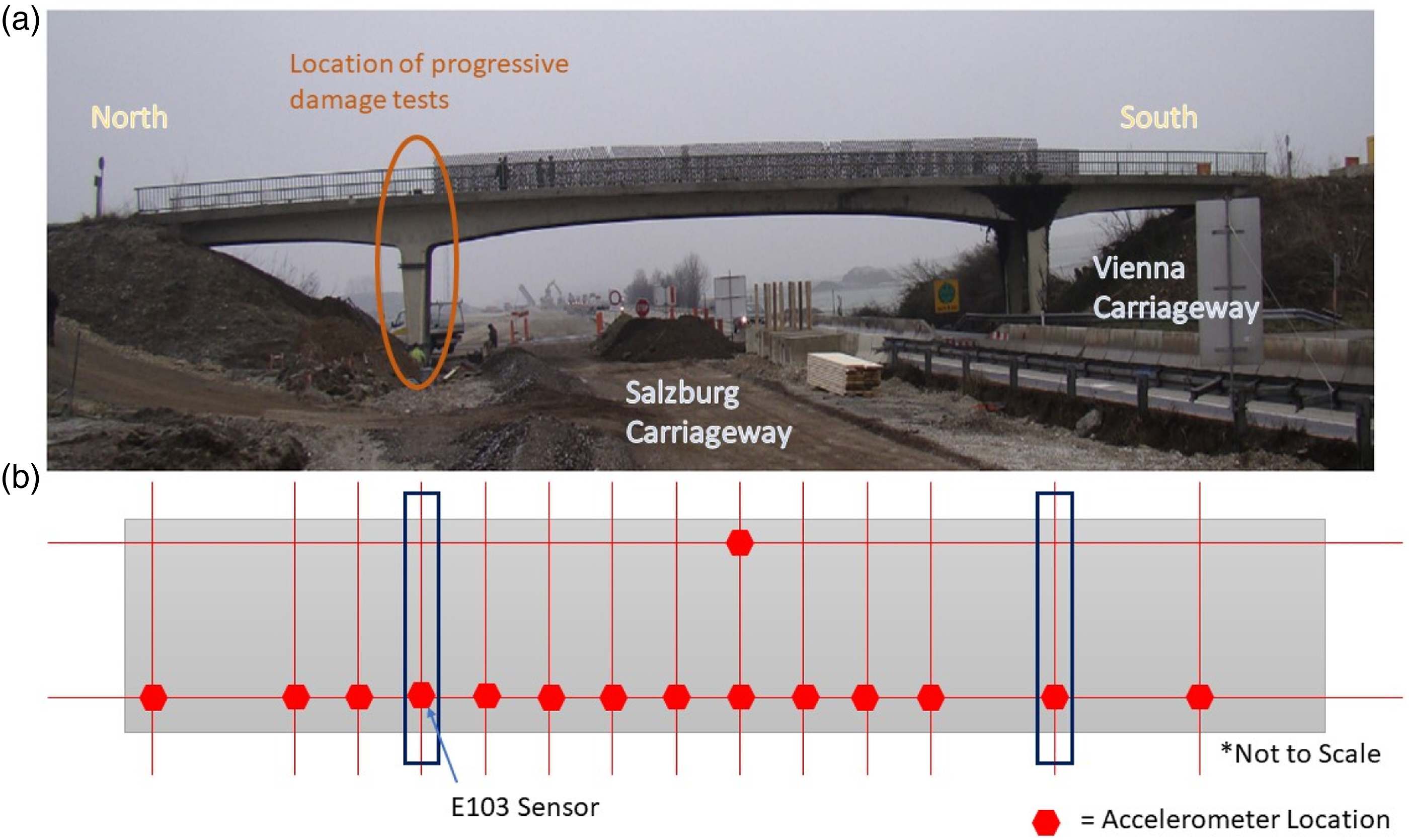
List of Minutes and Timeline
Timeline of events, S101 bridge dataset.
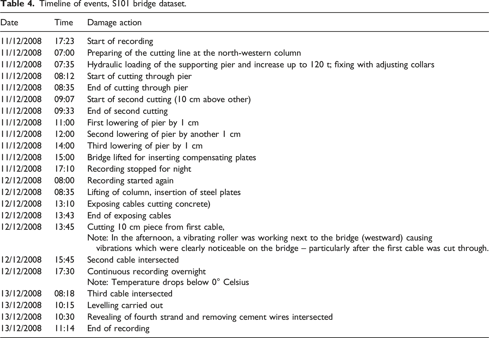
This event timeline is organised into 12 separate sequences which will be analysed as separate damage classifications. Each sequence corresponds to a damage state caused by an action on the bridge and any subsequent monitoring before the next action. These were obtained from detailed notes in Ref. [98].
There is a missing sequence of data is present in the timeline during Class F as recording was paused overnight from 17:10 to 08:00.
Z24 Bridge
The Z24 dataset was recorded from a pre-stressed concrete, 14-30-14 m span, highway bridge in Switzerland, Figure 3. Two rows of three pinned concrete columns are supporting the bridge at the endpoints and two concrete piers clamped into the girders are situated at the end points of the main span. Although there were no known structural problems with the bridge, it had to be demolished because a new railway next to the highway required a bridge with a larger side span. A detailed description of the monitoring can be found in Ref. [38]. (a) Z24 bridge (b) close up view of bridge (c) longitudinal section and plan view of Z24 bridge.
99
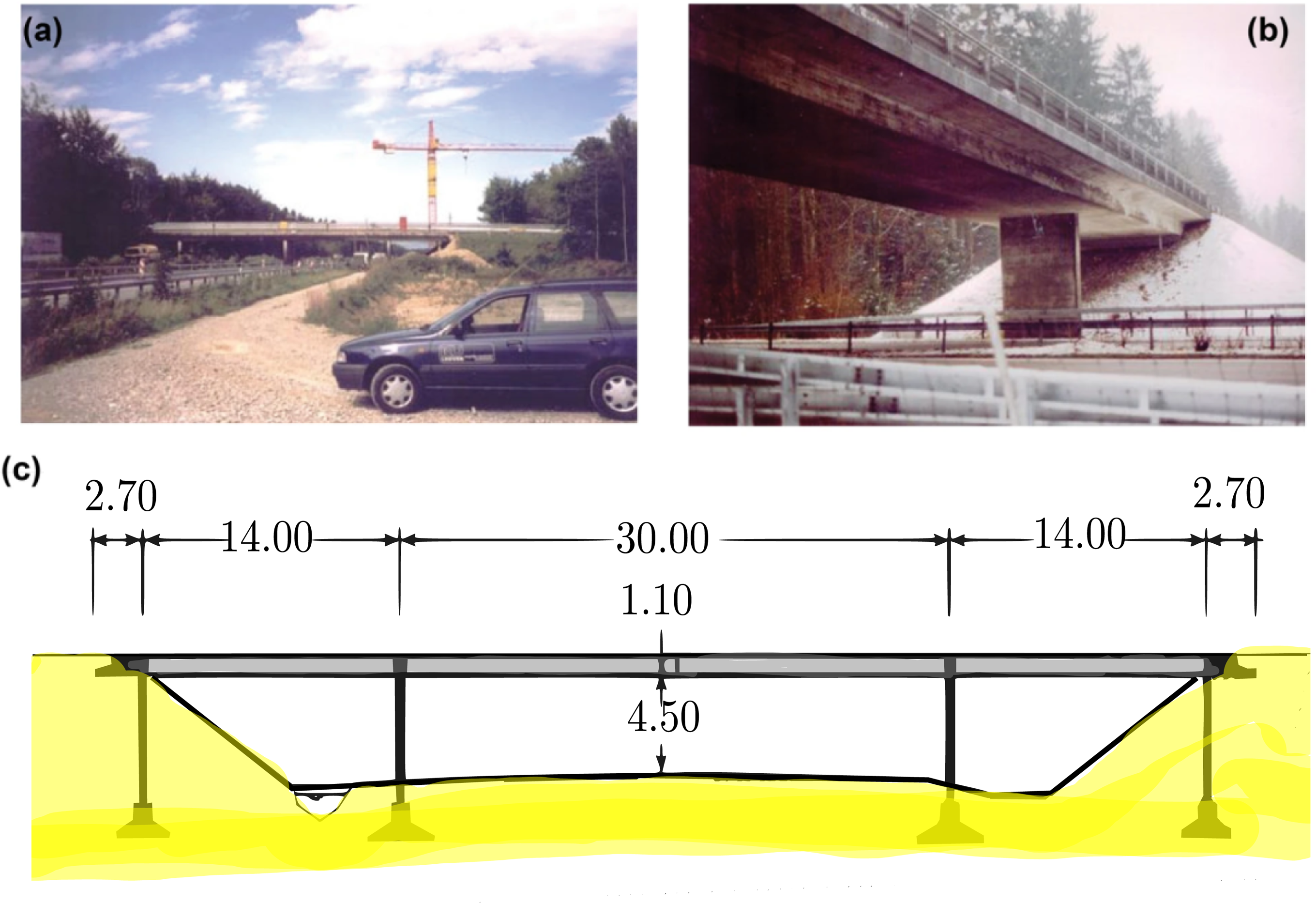
Prior to its demolition, it was monitored for almost an entire year, from 10th November 1997 to the 10th September 1998, using a network of accelerometers and environmental sensors measuring air temperature, soil temperature, humidity, etc. 99
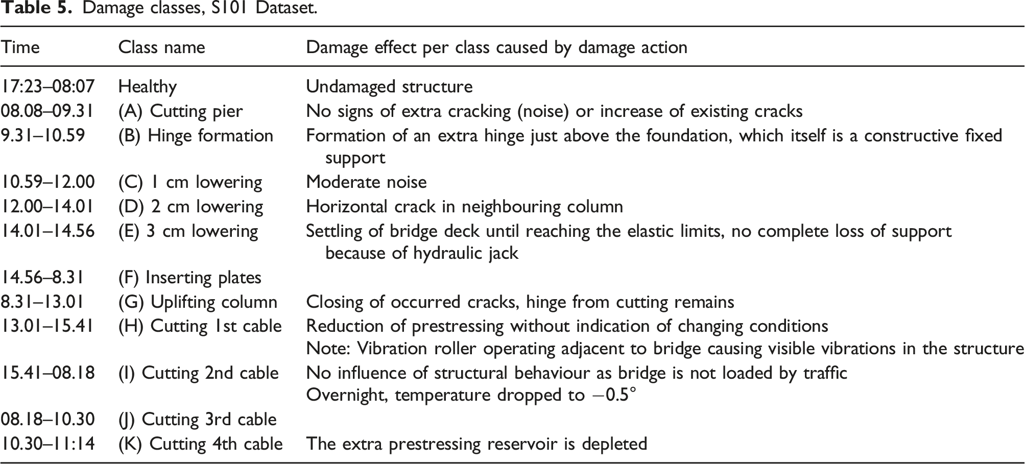
Damage classes, S101 Dataset.
Due to the lack of long term monitoring data where a healthy structure experiences damage, the Z24 dataset has become the benchmark dataset in the field of SHM over the last 20 years.6,17,37,91,100–102
PDT Monitoring Data
Progressive Damage Tests (PDTs), Z24 bridge. 81
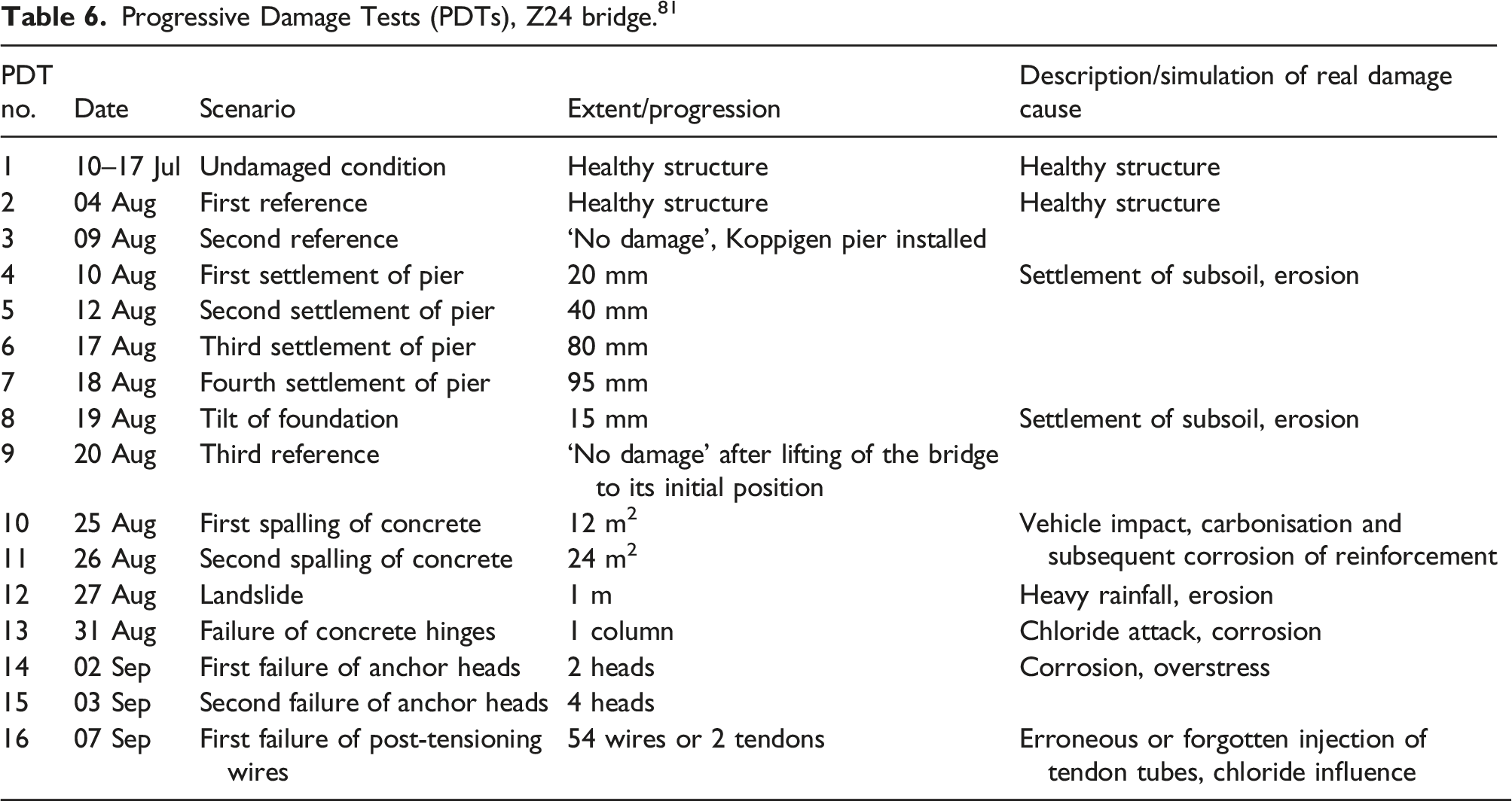
The installation of the testing apparatus involved serious changes in the structure. As a result, three of the PDTs are described as reference states against which the other PDTs are compared. To facilitate reversible settlement of the pier, jacks were installed on the pier at the Koppigen end of the bridge. PDTs 3–6 involved lowering of the pier which produced some cracking. After this, the pier was returned to its original position. In PDT 7, the foundation was rotated. The foundation was then returned to its original position before a third reference measurement was taken, PDT 8. PDTs 9–16 involved irreversible, cumulative damage (Figure 4). Progressive damage test sensor layout.
For each PDT, nine test setups were deployed with 33 acceleration time-series from various sensors collected. Data was sampled at 100 Hz and a total of 65,568 samples were measured for each setup. There were five common time-series between the setup tests: R1-V, R2-T, R2-V, R2-L, and R3-V. R1, R2, R3 are the location of sensors and V, T, L denote the sensor orientation. The layout of the accelerometers across the structure for the PDTs is shown in Figure 4 with R1, R2 and R3 denoting three reference locations. For each PDT, the bridge was tested with both ambient (Ambient Vibration Testing AVT) and forced (Forced Vibration Testing FVT) excitation from a shaker.
Analysis of S101 Bridge
As a baseline for the feature selection methods, the classification models are trained and tested on a full feature set. Next, each of the feature selection methods is applied to the dataset. The classification models are re-trained and tested using the reduced feature set obtained from each feature selection approach. Taking into consideration the motivation for edge feature extraction, the optimal feature set is the one which maximises the classification prediction performance with the minimal number of features.
Feature Estimation
For each accelerometer statistical time domain, temporal time domain and spectral time-frequency domain features are extracted using the Time Series Feature Extraction Library (TSFEL) in python. 71 A minute window was applied to the 500 Hz data leading to each feature being calculated over 30,000 datapoints.
Sixty one feature types were extracted from each accelerometer as in Appendix 1, Table 27. In Refs. [29] and [103], only the frequency range between 0 and 18 Hz was considered as this is where the first five modes can be identified. To restrict the volume of FFT mean coefficients computed for a sampling frequency of 500 Hz, in this analysis, only the FFT mean coefficients from 0 to 30 Hz are included in the analysis.
With FFT mean coefficients from 0 to 30 Hz and multiple MFCC, LPCC and wavelet coefficients, there are 141 individual features in total. The results presented are for sensor E103. This sensor was located nearest to the bridge column where the damage actions were undertaken.
The classification and feature selection methods outlined in the methodology are applied to this feature set to identify a subset of features which optimise the classification prediction of the different damage classes.
Classification
The damage class sizes in the S101 data are highly imbalanced. Imbalance occurs when some classes have a low proportions of data relative to the other classes. To account for class imbalance, weighted classification prediction performance metrics are used to evaluate the classification models for the S101 dataset.
For k-fold cross validation, the challenge with an imbalanced dataset is that some training folds will not contain any datapoints from certain minority classes and majority classes will be overrepresented. Therefore, a stratified cross validation procedure is implemented for the S101 dataset. Stratification samples test data from each class, maintaining the relative class sizes for the training and test splits and ensuring that each damage state is represented in each fold. A standard 5-fold stratified cross validation is chosen which results in an 80–20 train-test split across each fold and each damage state. The data is not shuffled so that the time sequence within each class is maintained.
Hyperparameter Optimisation
To identify the optimum hyperparmeters for each model, a 5-fold stratified cross-validation grid search method is first deployed on the S101 dataset.
Classifier hyperparameters.
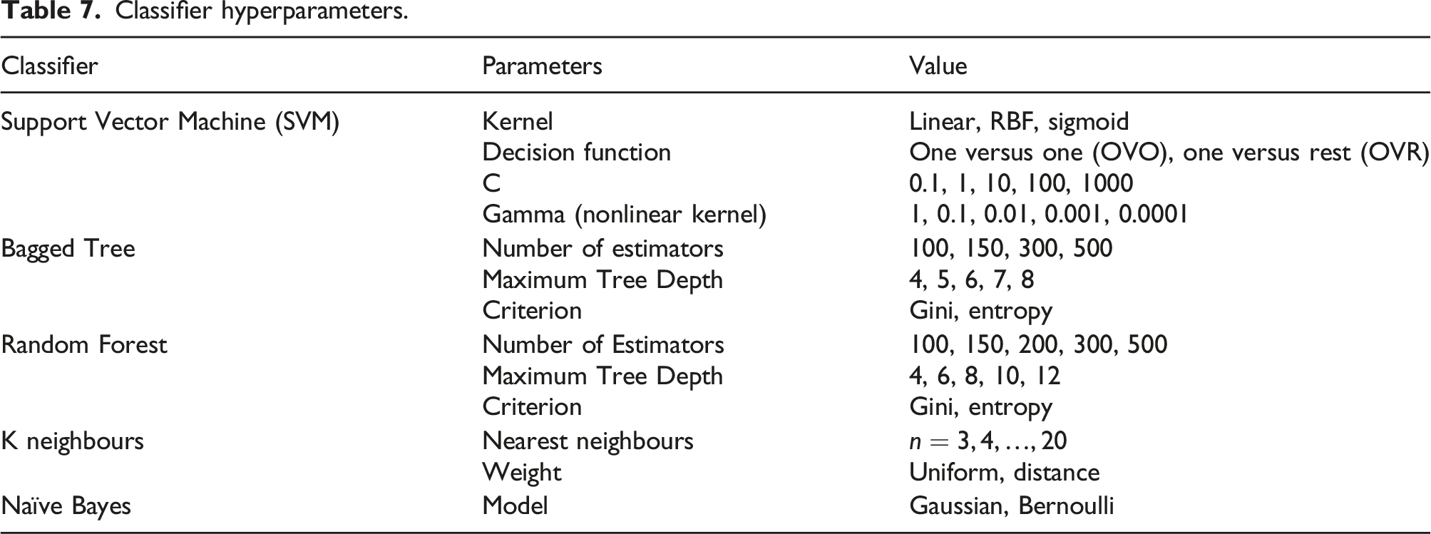
The size of the hyperparameter grid is determined by the range and combination of hyperparameters chosen for each model.
The grid search cross validation procedure is used to identify the optimal hyperparameters of each classification model. Grid search cross validation is the most widely used method for optimising the parameters of a machine learning classifier. 104 This method generates an exhaustive list of candidate models from a grid of parameter values. The chosen hyperparameters are then chosen are from the model with the best classification performance.
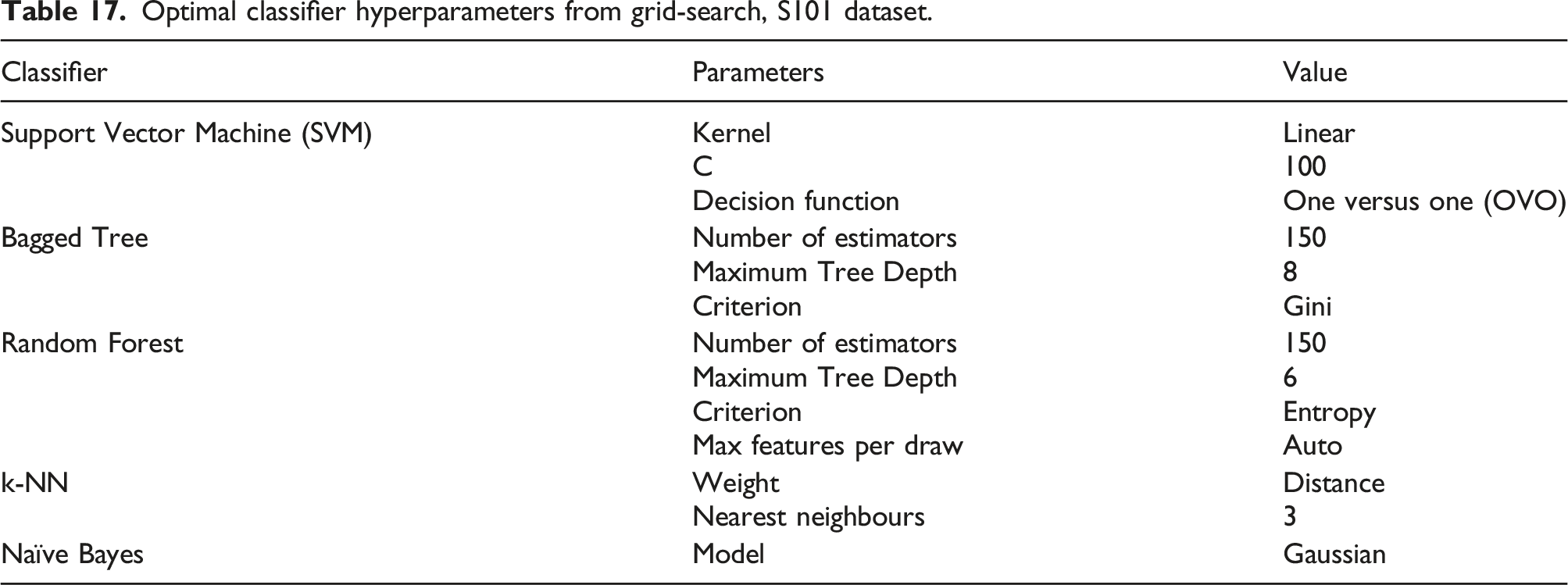
For example, using the parameters of the Support Vector Machine in Table 7, three grids of parameters must be explored for candidate models. 1. Grid one contains the linear kernel and the list of C values (0.1, 1, 10, 100, 1000) 2. Grid two contains the RBF kernel and the cross-product of the C values (0.1, 1, 10, 100, 1000) and the gamma values (1, 0.1, 0.01, 0.001, 0.0001) 3. Grid three contains the sigmoid kernel and the cross-product of the C values (0.1, 1, 10, 100, 1000) and the gamma values (1, 0.1, 0.01, 0.001, 0.0001)
These grids are run once for the one versus one (OVO) decision function and again for the one versus rest (OVR) decision function.
Optimal classifier hyperparameters from grid-search, S101 dataset.
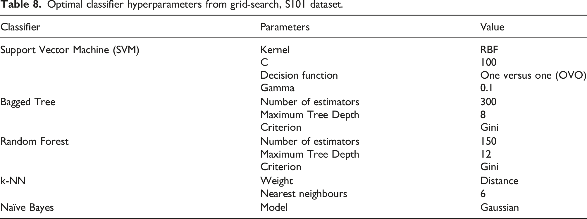
The parameters that maximise the classification prediction performance of the entire feature set are chosen in advance to avoid overfitting of the training dataset and to ensure comparability of models across different cross validation folds for each feature selection method.
Full Feature Set
Classifier performance S101, full feature set, 5-fold stratified cross validation.
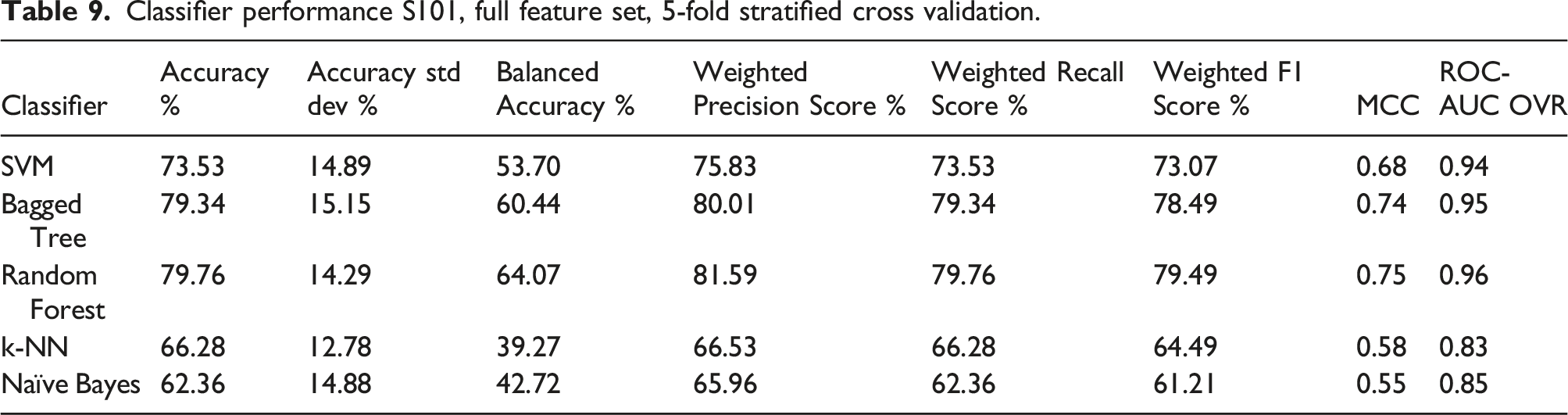
ROC-AUC is the Area under the curve of the receiver operating characteristic. This is a binary metric which is computed in a one versus rest (OVR) manner.
Full feature set S101, random forest five stratified cross validation folds.
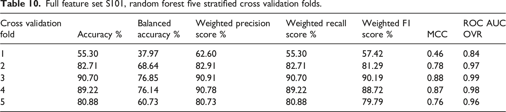
The highest overall performance is achieved in fold 3 and the worst in fold 1. The high standard deviation across the folds is caused by the significant difference in the classification performance of the first fold compared to the next four folds.
Figure 5 shows a confusion matrix for fold 1, the worst performing fold. The majority of misclassifications are occurring between successive damage states with values being misclassified as the previous damage state. The misclassification in this fold demonstrates the challenge involved in classifying damage states from a sequential dataset. For an unshuffled stratified sample, the unseen test data for the first fold is from the beginning of each class. The point at which one class ends and another begins was defined based on observations of the technicians on site. As each class includes data moving between damage states, it is expected that there could be some misclassification at the regions between classes, particularly for classes of similar damage states. This is particularly evident for damage states H, I and J which all involve the cutting of cables in the structure. Of primary importance for SHM is the separation between healthy and damage states and the reduction of false alarms. For the Healthy state, 98.3% of the unseen healthy data is being correctly predicted and the False Negative rate for the Healthy state is 93%. Therefore, despite the poor overall classification prediction for this fold, there classifier is clearly distinguishing between the Healthy state and the damage states. Full feature set S101, confusion matrix, random forest, fold 1.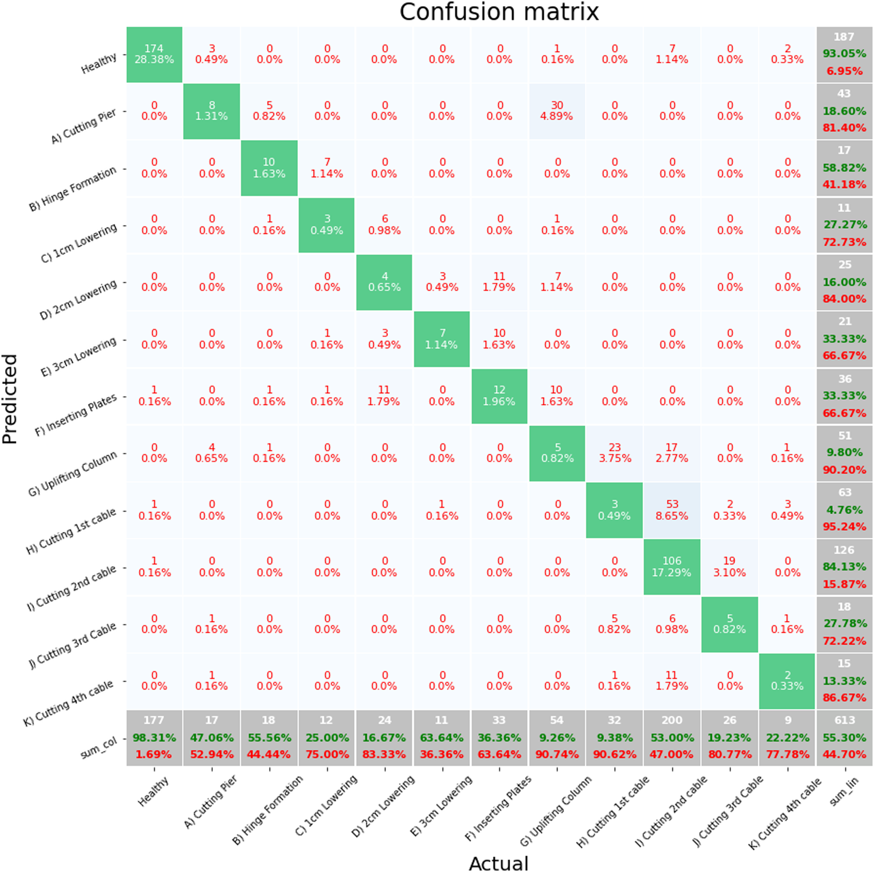
Figure 6 shows a confusion matrix for fold 3 which has the best classification performance from any of the folds. It is of note that for this fold, the test data was sampled from the middle of the class. As with fold 1, the majority of miss classifications are between damage states B and C and damage states G and H. Both cases are the border between the beginning of the pier lowering and cable cutting, respectively. Full feature set S101, confusion matrix, random forest, fold 3.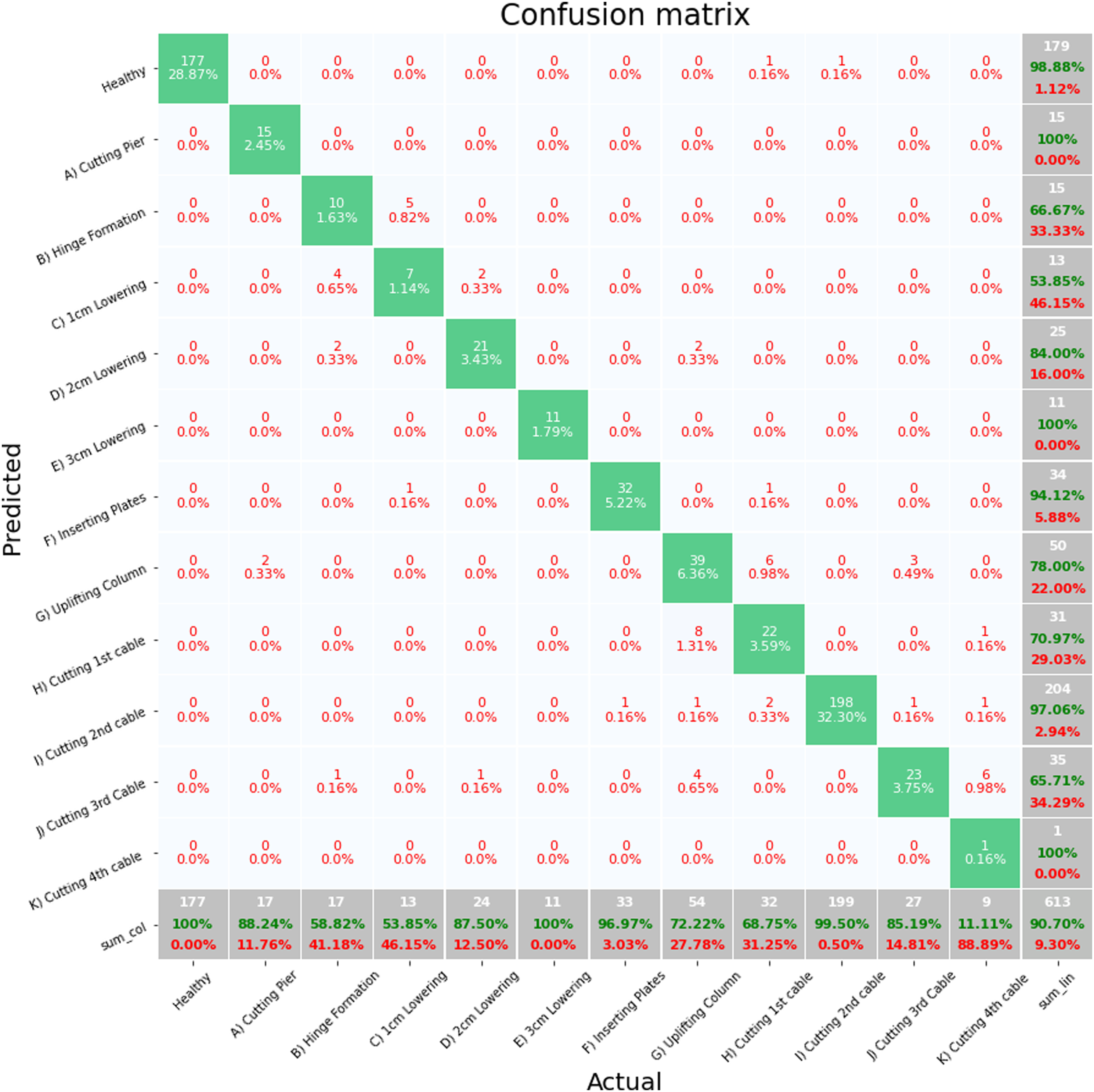
One of the concerns with an imbalanced dataset is that a classifier may learn to improve prediction performance by randomly assigning datapoints to majority classes. The confusion matrices show that this is not the case as the majority of miss classifications across the folds are when the unseen test data is at boundaries between classes, particularly between the damage states G, H, I and J where cables were cut.
The poor balanced accuracy scores from Table 10 are heavily influenced by classes such as damage state K which has a very poor classification prediction performance across each of the folds. This is not unexpected as damage state K has a small number of datapoints and the damage event, fourth cutting of cable, is very similar to the previous three damage states, J H and I with higher numbers of datapoints in their class.
Although each of the metrics in Table 9 and Table 10 differ in their values, they all have the same variation across each of the classes. As it is representative of both the precision and recall, the weighted F1 score will be used as the metric by which the various feature selection methods are compared and evaluated against the full feature set baseline.
Feature Selection
Next, the four feature selection methods are applied in combination with each of the five classification algorithms to identify the minimum feature sets that also maximise classification performance.
ANOVA F-Test
The top 80 features ranked by significance according to the ANOVA F-Test filtering method are shown in Figure 7. ANOVA F-Test, top 80 features.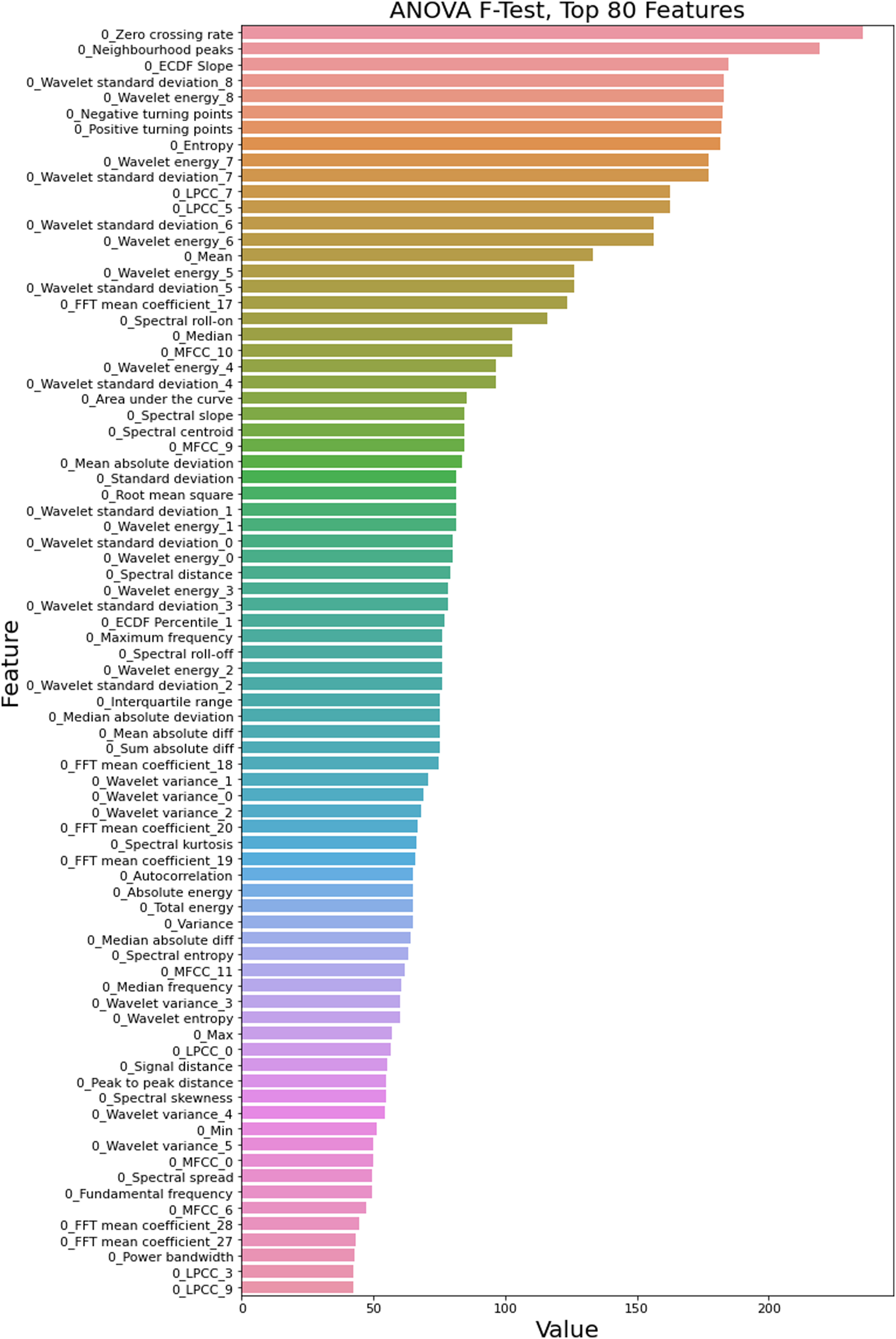
The x-axis shows the significance score from the ANOVA hypothesis test for the variance of each individual feature with different damage states. The y-axis shows the ranking of each feature based on its individual significance score.
The ANOVA feature selection method is a univariate method where each value’s relationship with the target classes are investigated individually before any classifier is applied. Figure 8 shows the variation in the weighted F1 score for each classification model with varying percentiles of ranked ANOVA features. The features are removed in a recursive manner as depicted in the methodology and the top percentile then modelled by the classifier. The figure shows 1%, 5% and 10% percentile increments of ranked features from 10% up to 100%. ANOVA ranked features, F1 score, S101 dataset.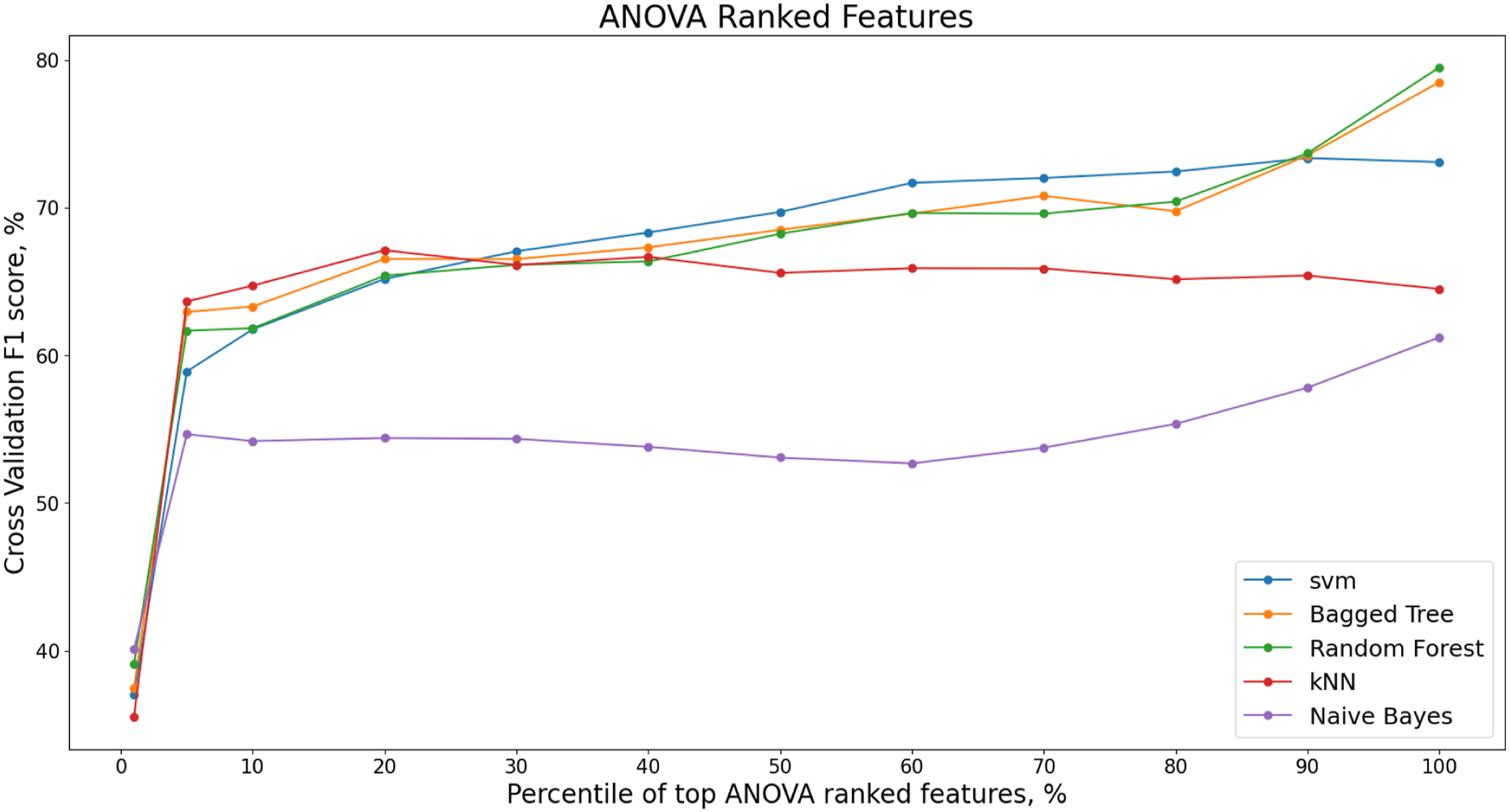
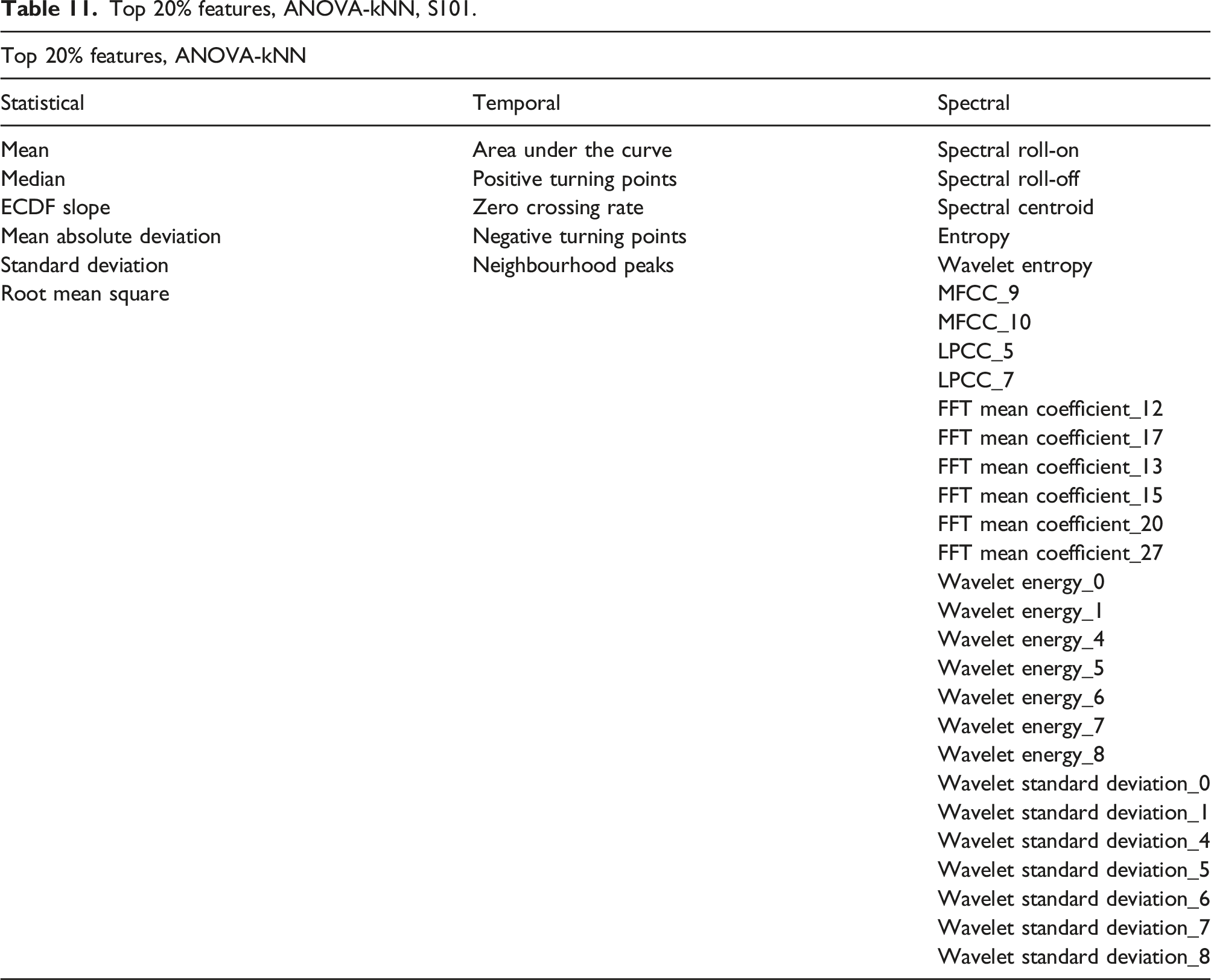
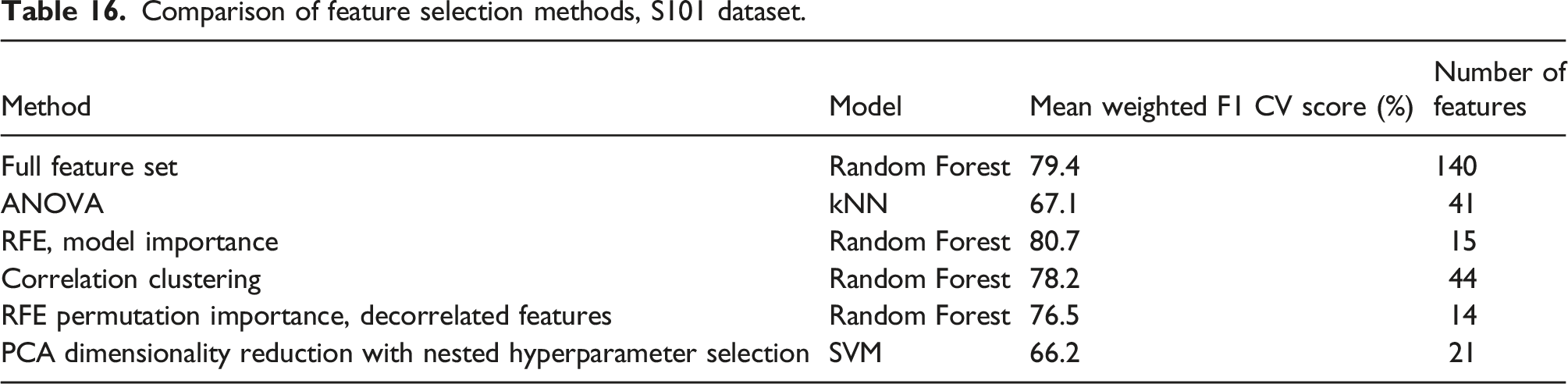
Although the Random Forest model has the highest overall F1 score, this is only after 90% of the ANOVA ranked features are included. The minimum number of features for the highest F1 score is achieved at 20% of the ANOVA ranked features for the kNN model. The number of features for the ANOVA-kNN model at 20% is 41 with an F1 score of 67.1%.
Top 20% features, ANOVA-kNN, S101.
RFE with Model Importance
Features can also be ranked based on their intrinsic importance in the modelling of the training data by the classification algorithms. This provides an understanding of how the machine learning models are predicting the damage states.
The intrinsic model importance of features can be identified for the SVM, Bag Tree and Random Forest models. The kNN and Naïve Bayes model have no intrinsic method for ranking features.
The recursive feature elimination is implemented for increments of 5% of features ranked by model importance. Varying percentiles of features are shown in Figure 9 for the SVM, Bagged Tree and Random Forest models with the corresponding mean weighted F1 score from the five cross validation folds. Recursive Feature Elimination (RFE) for varying percentiles of features ranked by model importance, S101 dataset.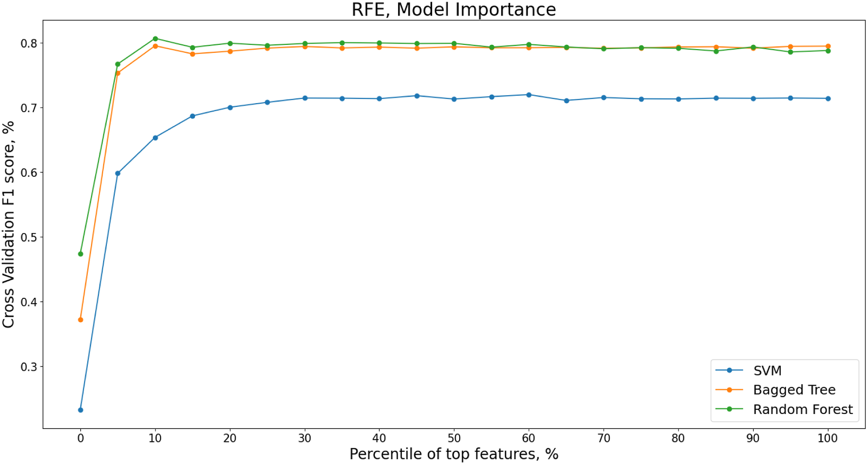
Selected features from top 10% of RF-RFE model, S101 dataset.
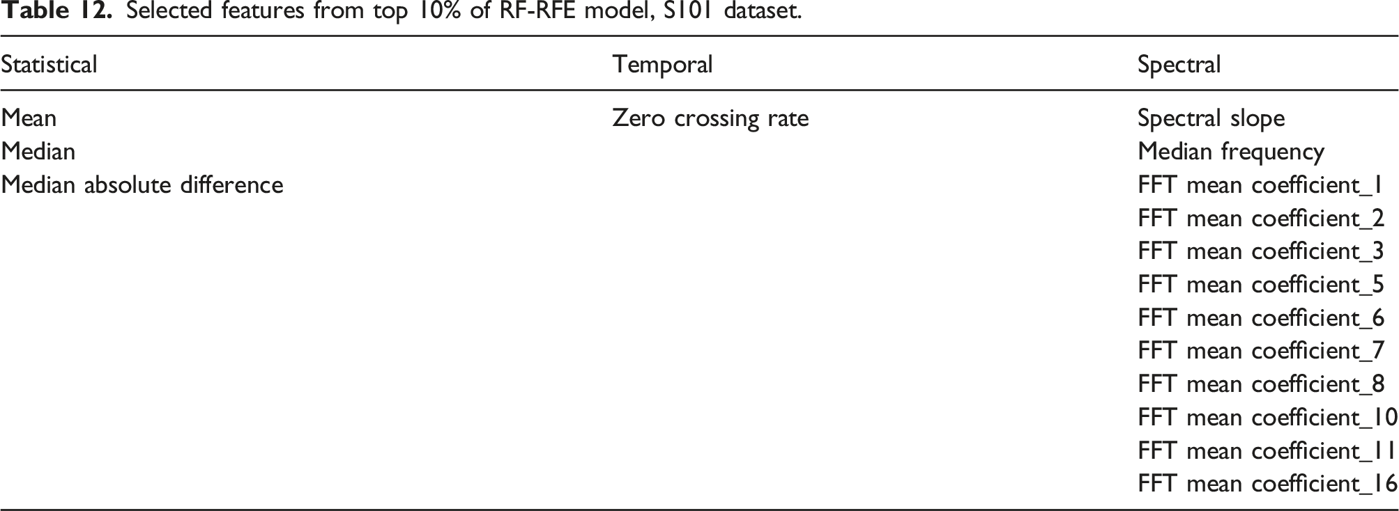
The F1 score is higher for these 16 features than when the entire feature set is included.
Ten out of the 16 most important features to the training of the random forest model are FFT mean coefficients from 1 to 16. It is possible that high model importance is being assigned to the FFT mean coefficients between 1 and 16 Hz due to their high correlation rather than their individual importance. When a training dataset contains large groups of correlated features, this can confound model interpretation with large groups of predictive and important features being masked and falsely appearing irrelevant. 105
Correlation Clustering
A Spearman correlation plot, Figure 10, shows the high correlation present in the statistical time domain, temporal time domain and spectral time-frequency domain features from across the entire S101 dataset. The lighter the colour, the higher the correlation with darker colours indicating negative correlation. Spearman correlation plot.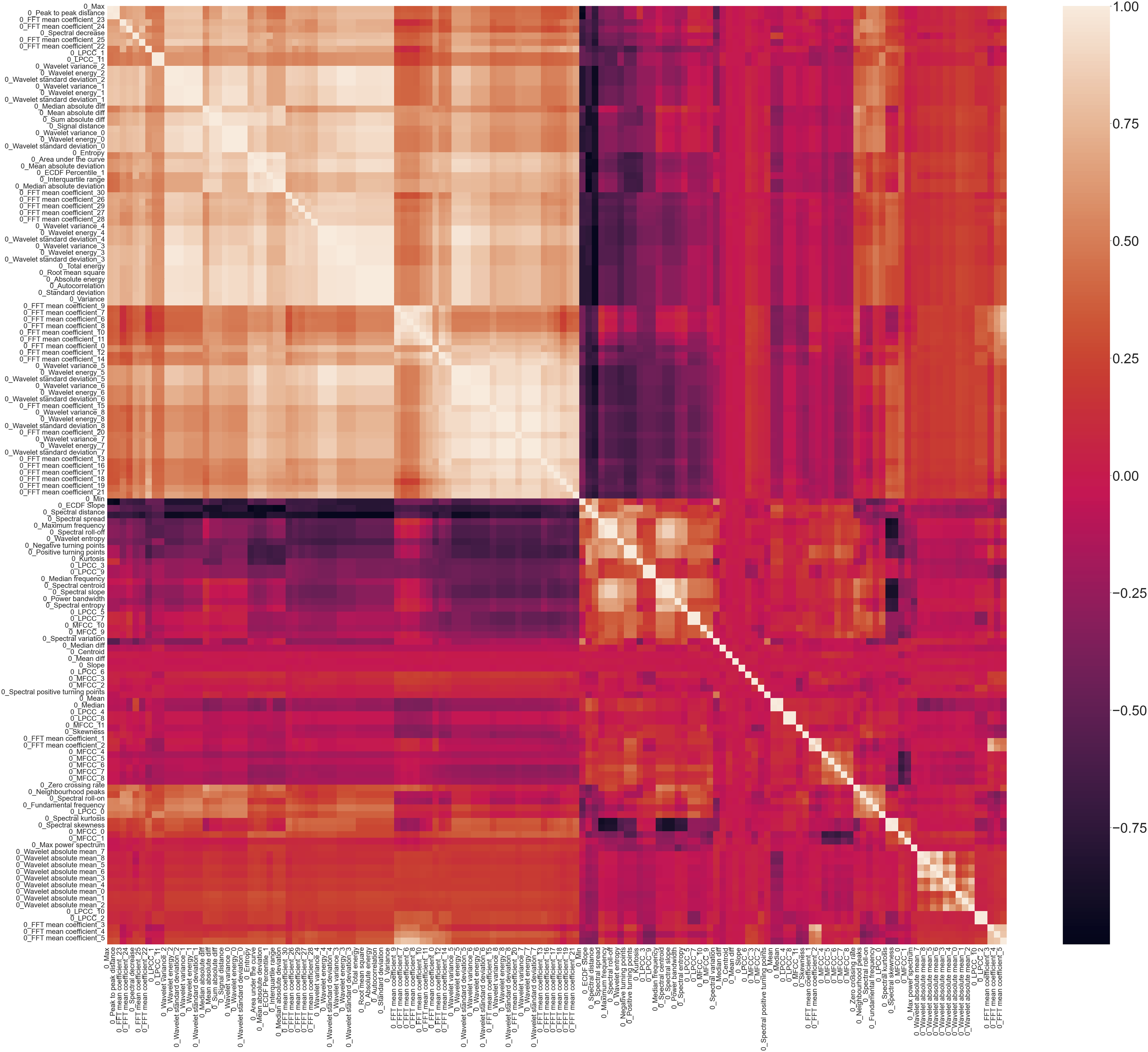
To reduce the number of features and the presence of multicollinearity in the dataset, hierarchical clustering is applied to the spearman rank-order correlations shown in Figure 10. A dendrogram, Figure 11, provides a visual representation of the hierarchical clusters for the feature set from the S101 dataset. Dendrogram of features, S101.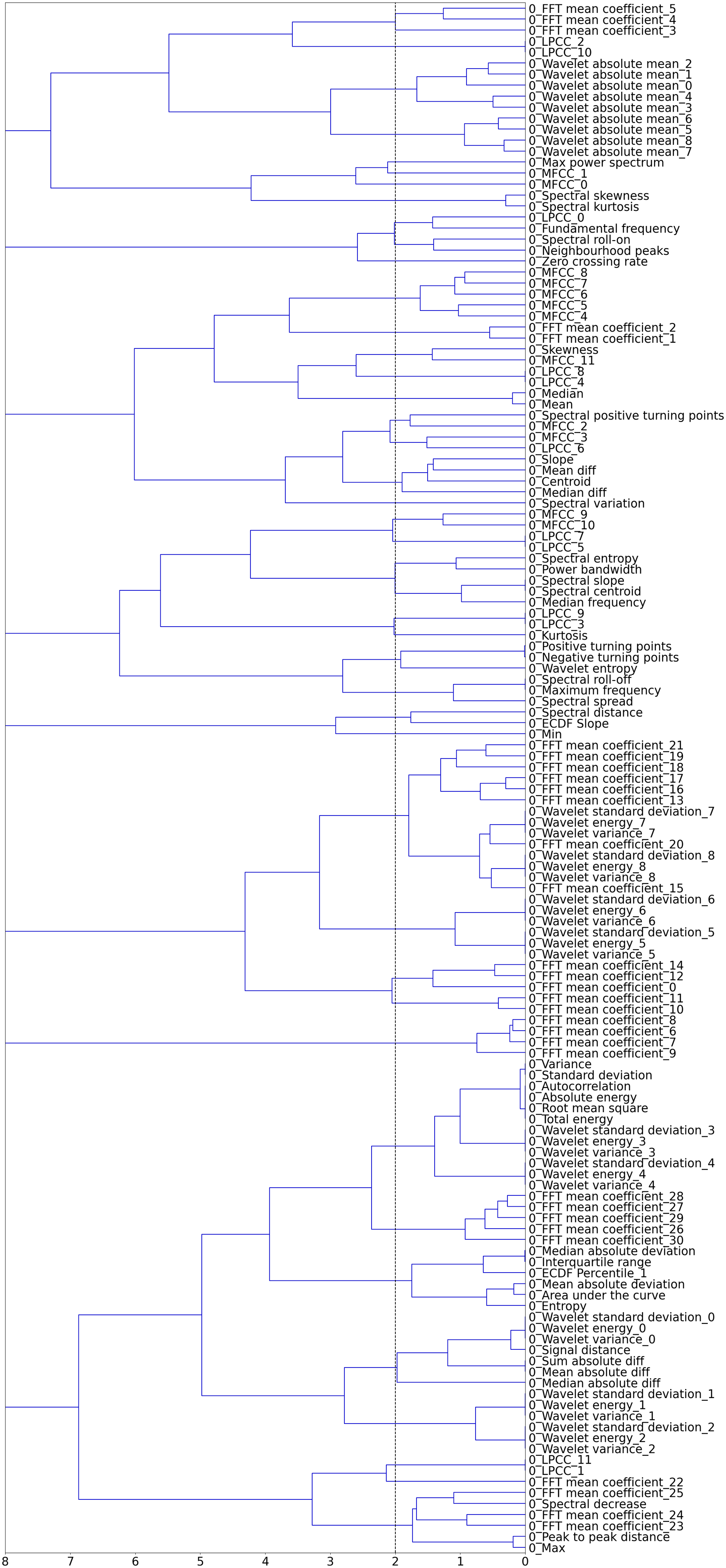
The x-axis of the dendrogram shows the distance between each of the clusters. The number of clusters decreases with increase in clustering distance. To reduce the correlated feature set, a threshold is set along the x-axis of the dendrogram and one feature is chosen from each cluster. Figure 12 shows how the performance of the classifiers varies with increasing hierarchical clustering distance thresholds (Figure 13). Varying F1 score for each classifier with increasing cluster distance thresholds, S101 Dataset. Recursive Feature Elimination (RFE) for varying percentiles of decorrelated feature set, ranked by permutation importance, S101 dataset.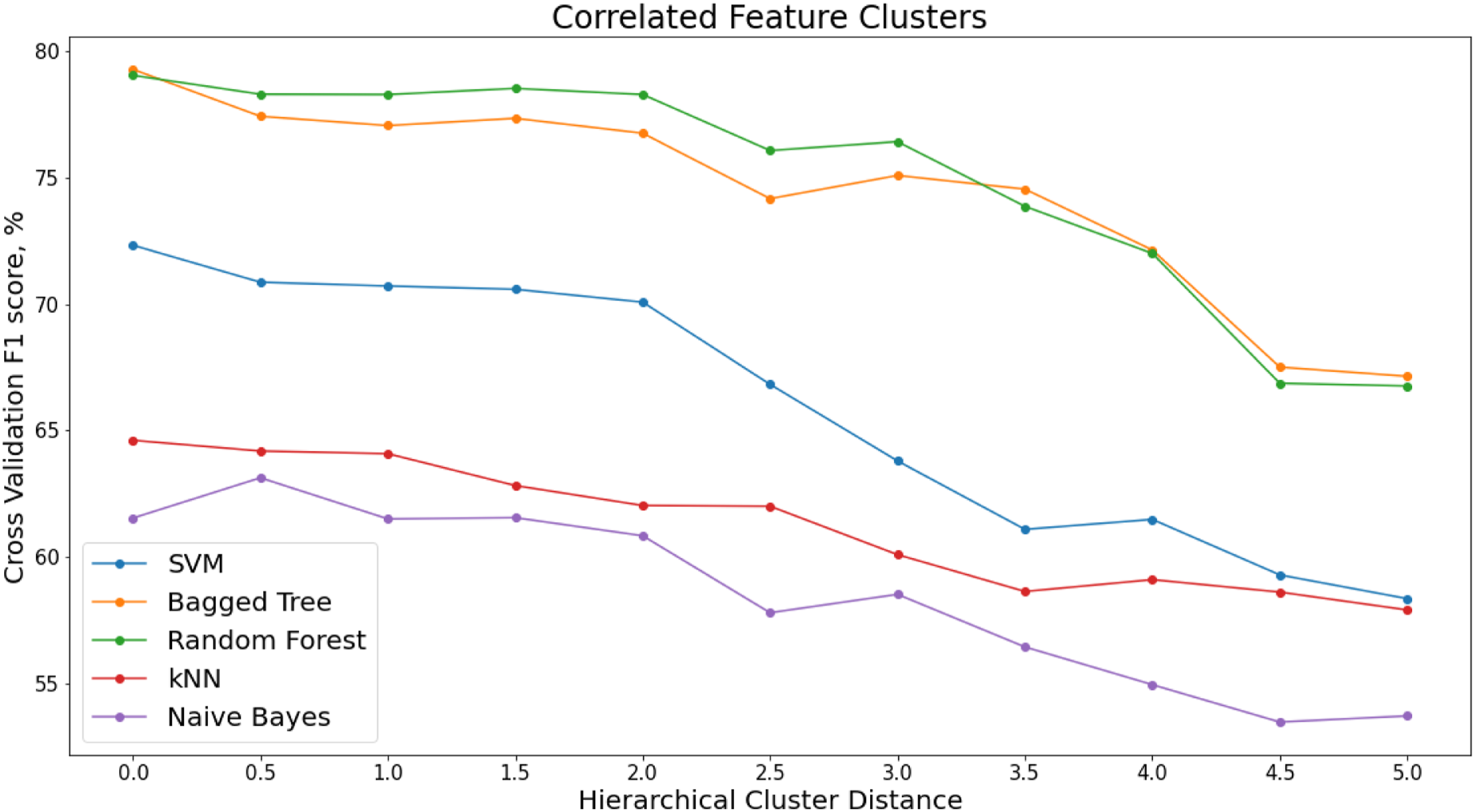
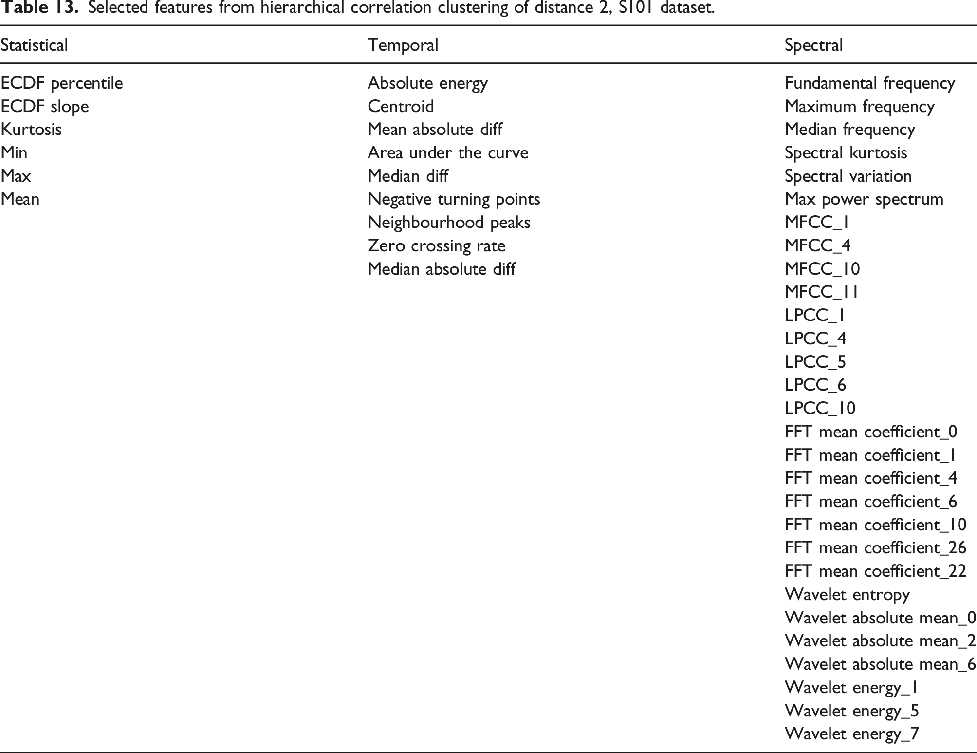
Selected features from hierarchical correlation clustering of distance 2, S101 dataset.
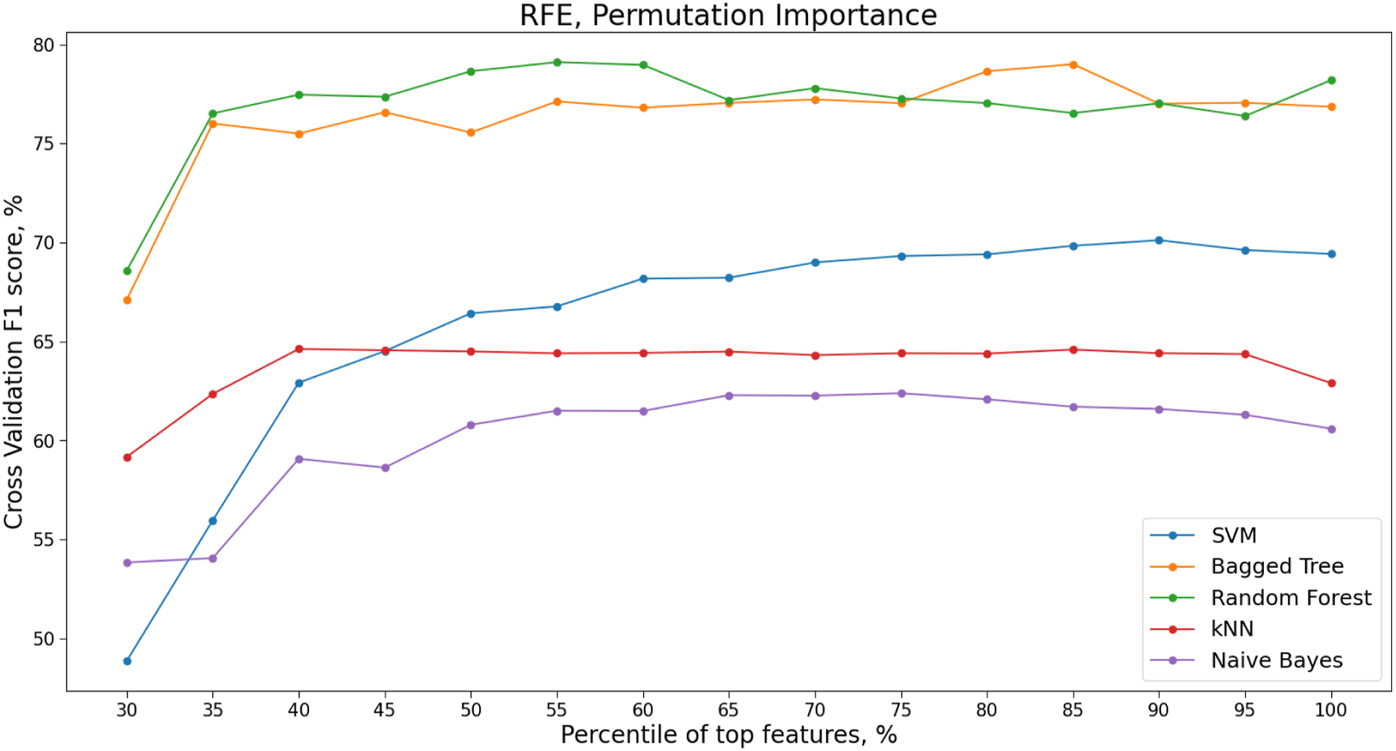
RFE with Permutation Importance
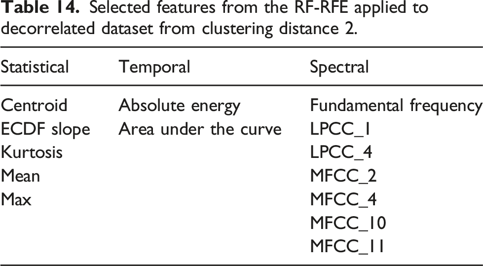
When features are collinear, permuting one feature will not have much effect on the model prediction performance as the same information can be obtained by the model from a correlated feature. RFE with Permutation importance is therefore applied to the decorrelated feature set presented in Table 13. The variation in F1 score with different percentages of permuted features from across the cross-validation folds is shown in Table 13.
Selected features from the RF-RFE applied to decorrelated dataset from clustering distance 2.
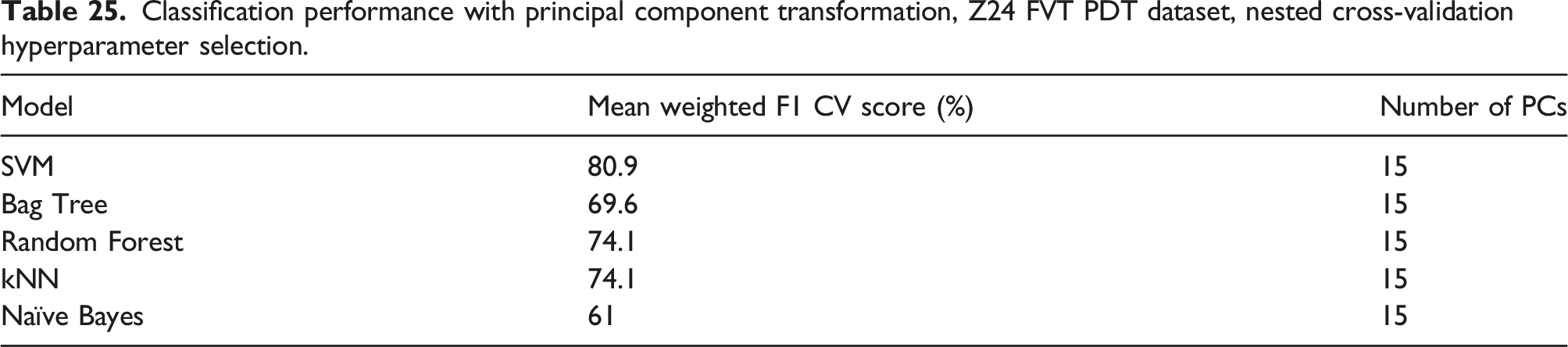
PCA Benchmark with Nested Hyperparameter Selection
As the standard dimensionality reduction technique used in SHM, Principal Component Analysis (PCA)106–109 is used as a benchmark for the classification performance of the reduced feature sets obtained in the previous sections for the S101 bridge dataset.
Principal component analysis, otherwise known as proper orthogonal decomposition, is a multi-variate method used to provide a linear mapping from the original feature dimension
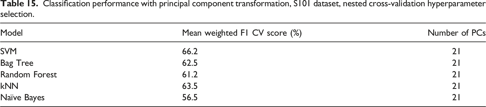
The full feature set of statistical time domain, temporal time domain and spectral time-frequency domain features is transformed using PCA; these principal comments are then used as the input features to each of the classification algorithms. The same 5-fold stratified cross-validation procedure is first used to train and test the classification model on the transformed feature set. For each fold, a training set of the feature matrix, composed of the extracted statistical time domain, temporal time domain and spectral time-frequency domain features are input into the PCA model. The number of principle components is chosen to model 90% of the variance within the training dataset.
Using the hyperparameters obtained from the full feature set, Table 8, to train the supervised classification models with the PCA transformed feature set would result in a substantial reduction in classification performance. As the PCA algorithm transforms the features to a lower dimension space, the relationship between the original feature set and the damage states or ‘classes’ has been significantly transformed.
Classification performance with principal component transformation, S101 dataset, nested cross-validation hyperparameter selection.
Comparison of Feature Subsets
Comparison of feature selection methods, S101 dataset.
Analysis, Z24 Bridge
In this analysis, PDTs 1–17 will be used as one full dataset. The PDT 1 reference state is considered to be the ‘Healthy’ state.
During PDT 2, the installation of the jack in the pier and associated safety work was carried out which caused a large change in the dynamic characteristics of the bridge. 6 This is therefore regarded as a Damage state.
From the 65,568 samples measured at 100 Hz from each setup. There were nine setups recorded over the day for each PDT. Features were extracted over windows of length 80 s resulting in 72 datapoint values per PDT.
Feature Estimation
The feature estimation follows the same procedure used in the analysis of the S101 bridge dataset. With FFT mean coefficients from 0 to 30 Hz and multiple MFCC, LPCC and wavelet coefficients, there are 141 individual features in total. The results presented are for reference accelerometer one near the Koppigen Pier (Figure 3).
The classification and feature selection methods outlined in the methodology are applied to this feature set to identify a subset of features which optimise the classification prediction of the different damage classes.
Classification
As opposed to the imbalanced S101 dataset, the class sizes in the Z24 dataset are of equal size. However, due to the sequential nature of the progressive damage tests and the 15 separate classes, standard 5 or 10 fold cross validation would be missing samples from classes within the training sets at each fold. To alleviate this, the data can either be shuffled or a stratified cross validation approach used. To maintain the sequential nature of the data within each class, a stratified 5-fold cross validation is again implemented for the Z24 PDT data. For the classification metrics, with a balanced dataset the weighted metrics will give the same results as the standard classification prediction metrics.
Hyperparameter Optimisation
Full Feature Set
The classification algorithms are first applied to the full feature sets from both the Ambient and Forces vibration test recordings.
Ambient Vibration Tests
Classifier performance, Z24, full feature set, 5-fold stratified cross validation, ambient vibration tests (AVT).
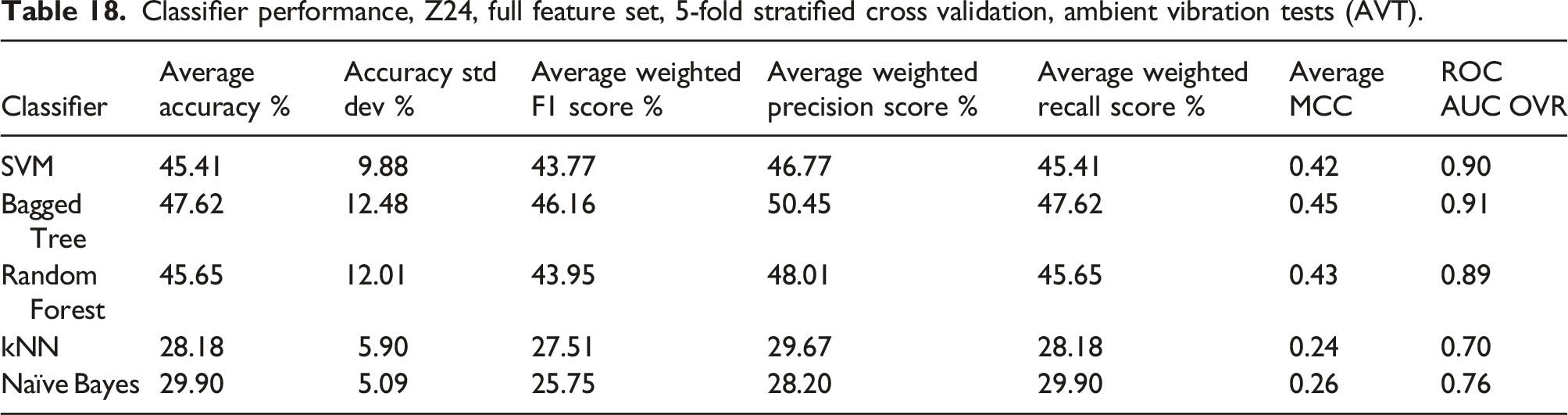
For the AVT, the only excitation on the structure was from one lane of traffic below the bridge.
Forced Vibration Tests
Classifier performance z24, full feature set, 5-fold stratified cross validation, forced vibration tests (FVT).
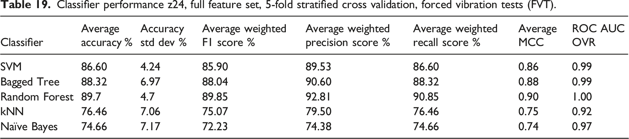
ROC-AUC is the Area under the curve of the receiver operating characteristic. This is a binary metric which is computed in a one versus rest (OVR) manner.
The Random Forest classifier has the overall best performance for the classification prediction metrics across the five folds. Each of the performance metrics has similar variation across each of the classification models.
Full feature set S101, random forest five stratified cross validation folds, FVT.
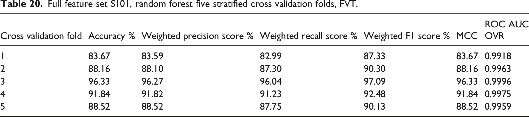
The highest overall performance is achieved in fold 3 and the worst in fold 1.
Figure 14 shows a confusion matrix for fold 1. Unlike the S101 dataset, the data from the z24 dataset is not continuous but distinct samples of data of 1 h. The unshuffled stratified sampling does however maintain the time sequence in the data so fold 1 contains data from the start of each progressive damage implementation. Stratified cross validation fold 1, random forest full features set, Z24 PDT FVT.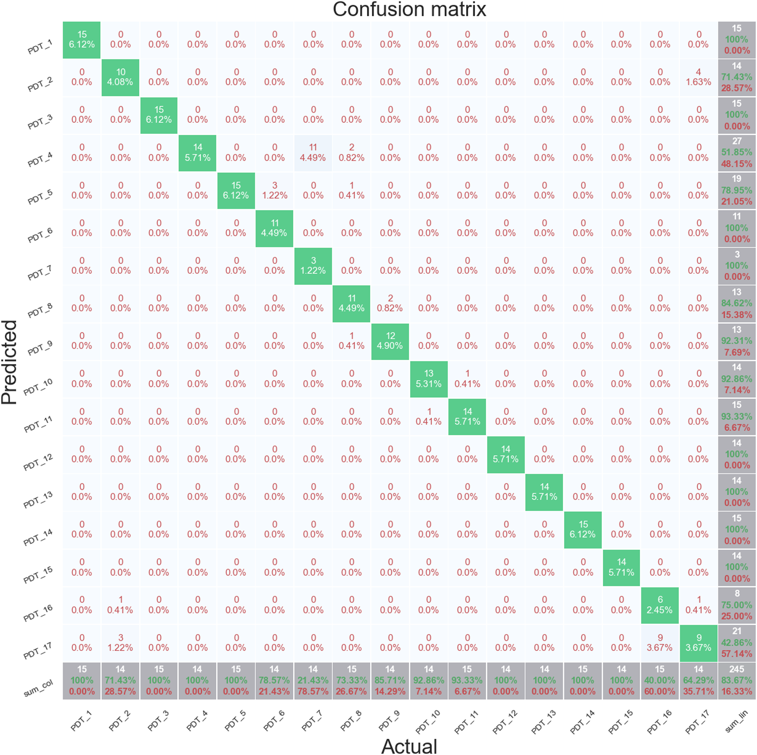
The majority of misclassifications are occurring between PDT 4 and PDT 7, the first and fourth settlement of the piers, respectively, and between PDT 15 and PDT 16, the second failure of anchor heads and first failure of post tensioning wires. This suggests that the effect of the cutting of the post-tensioning wires is not being identified in the signal features. The classification accuracy for the Healthy data, PDT 1, is 100%.
Figure 15 shows data from cross validation fold 3. This fold achieves an almost perfect prediction performance across all the folds with an overall accuracy score of 96.33%. The only misclassifications are between PDT 7 and PDT 5, the fifth and second settlement of the piers, respectively. The classification accuracy of the Healthy data, PDT 1, is also 100% for this fold. Stratified cross validation fold 3, random forest full features set, Z24 PDT FVT. Based on the classification results for the AVT and FVT, only the FVT data will be used in for the application of the feature selection methods.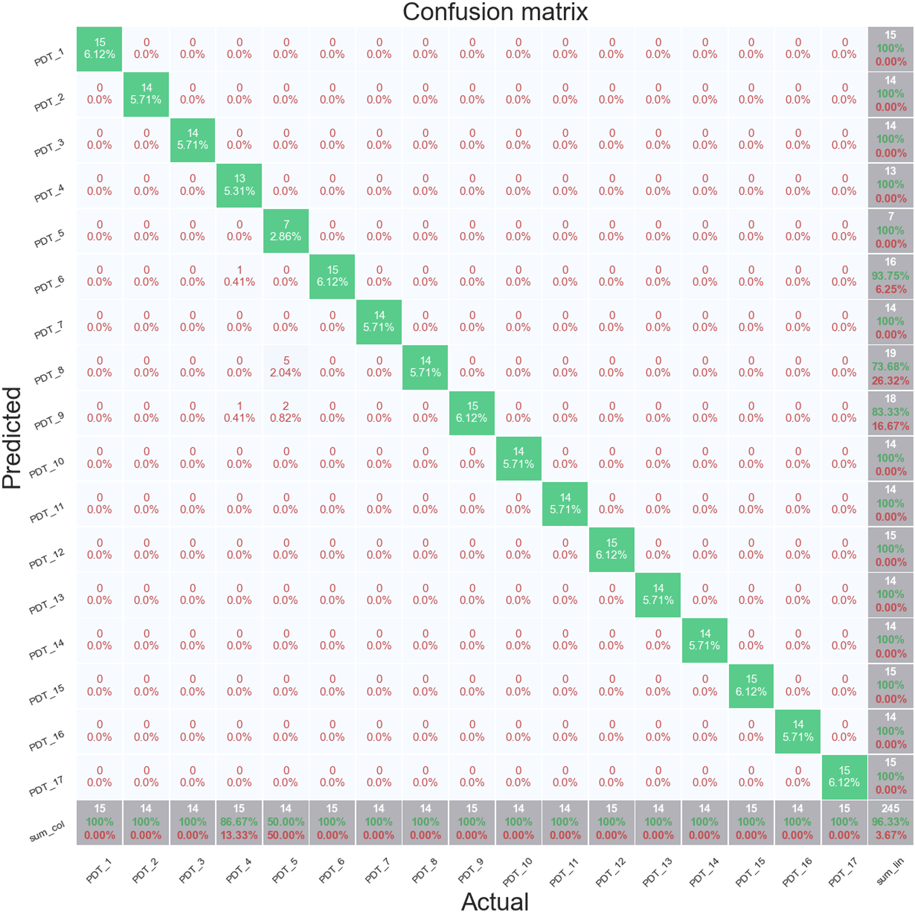
Feature Selection
Next, the four feature selection methods are applied in combination with each of the five classification algorithms to identify the minimum feature sets that also maximise classification performance.
ANOVA F-Test
Figure 16 shows the top 80 ranked features for the Z24 PDT FVT dataset. There is a clear difference between the variance in the first six features over the different damage classes compared to the rest of the features. ANOVA F-Test ranking of top 80 features, Z24 PDT FVT dataset.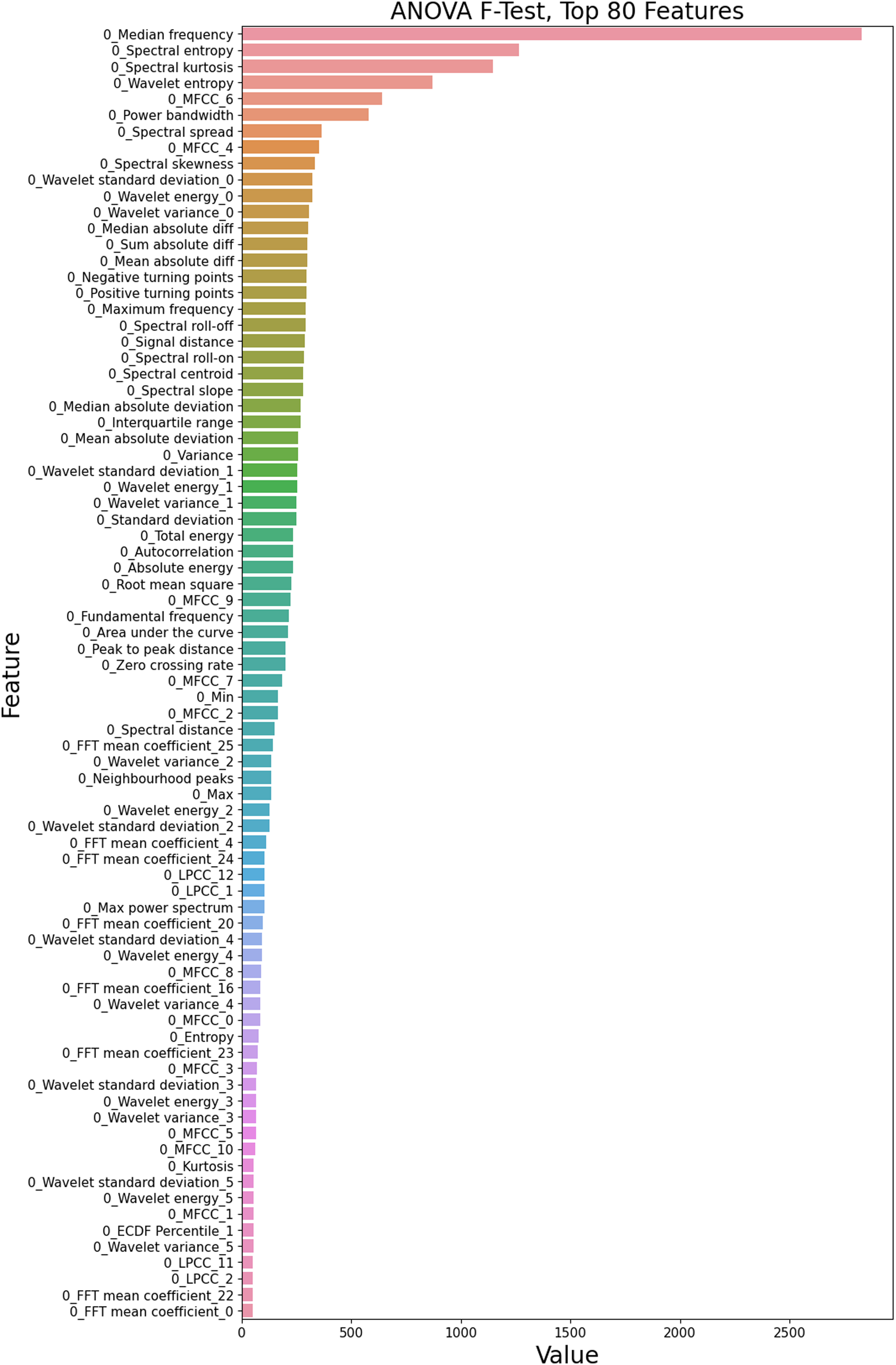
Figure 17 shows the change in F1 score for different percentiles of ANOVA ranked features for each classifier. ANOVA Ranked features, F1 score, Z24 PDT FVT dataset.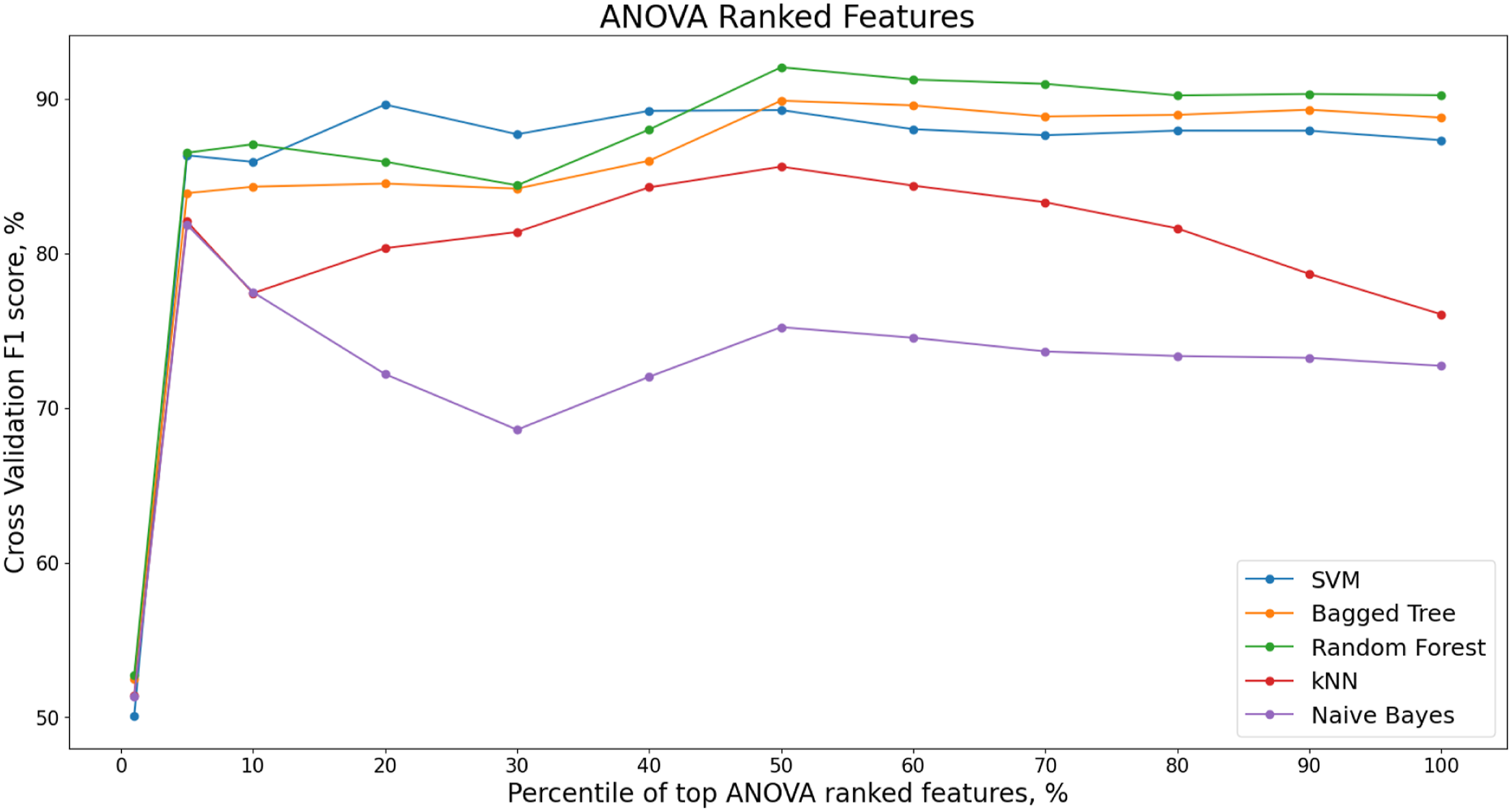
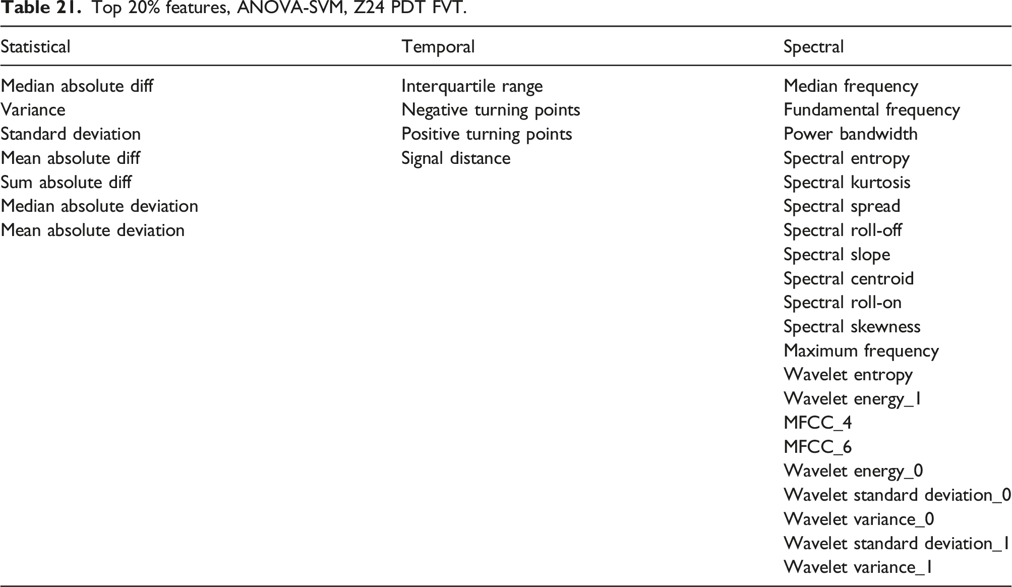
Top 20% features, ANOVA-SVM, Z24 PDT FVT.
RFE with Model Importance
The recursive feature elimination using intrinsic model importance for the SVM, Bag Tree and Random Forest models is next applied. Figure 18 shows the change in the cross validated F1 score for decreasing percentiles of features ranked by model importance. The RFE is implemented using increments of 5% of features. Recursive Feature Elimination (RFE) for decreasing percentiles of top features ranked by model importance, Z24 PDT FVT dataset.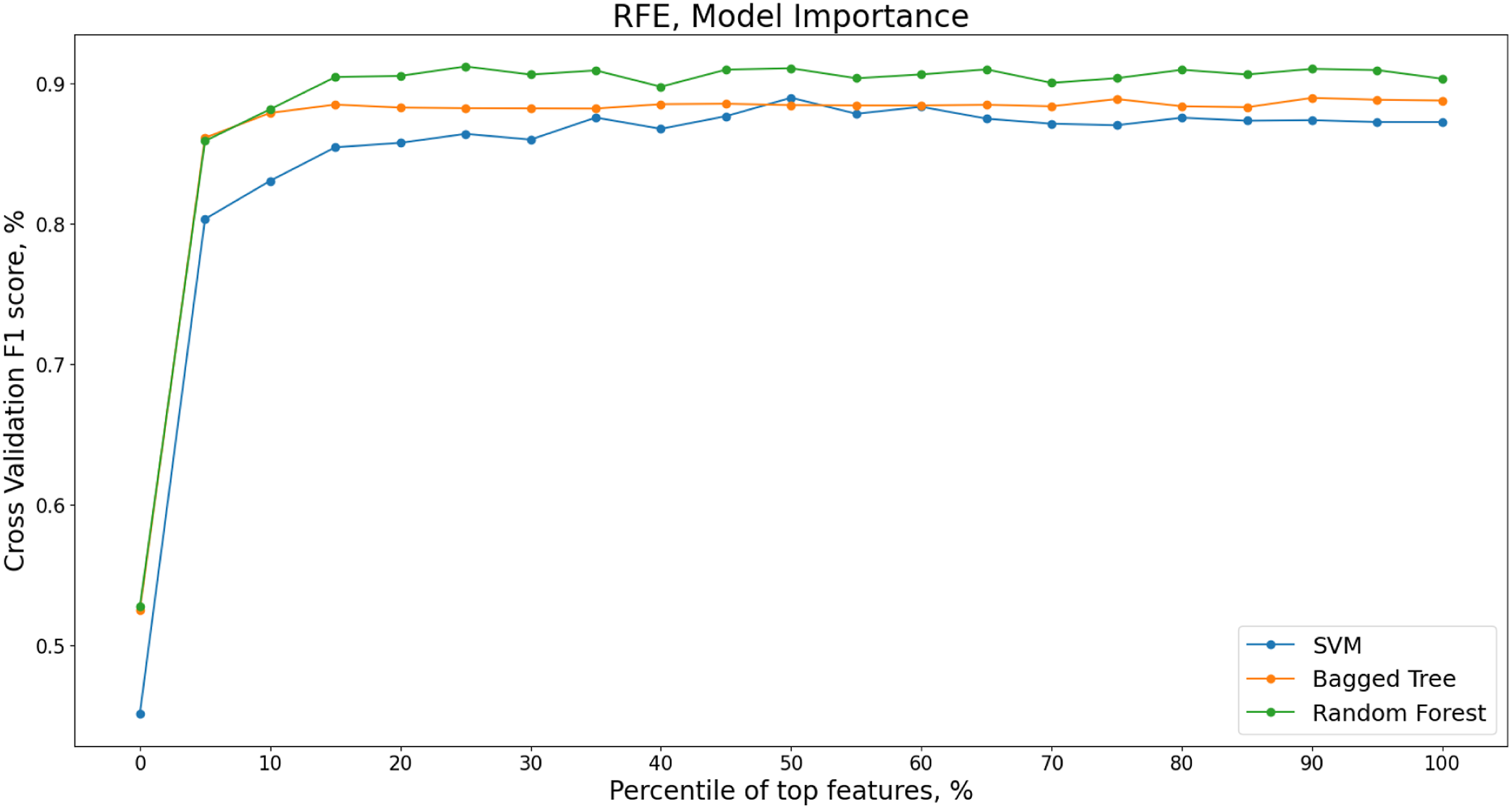
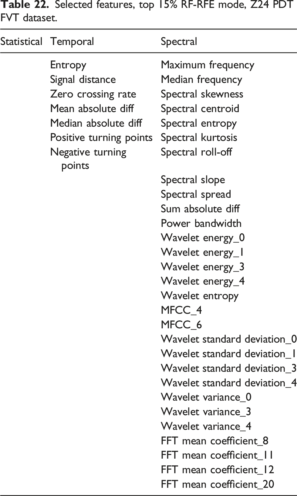
Selected features, top 15% RF-RFE mode, Z24 PDT FVT dataset.
Correlation Clustering
A Spearman correlation plot, Figure 19, shows the correlation present in the statistical time domain, temporal time domain and spectral time-frequency domain features from across the entire Z24 PDT FVT dataset. The lighter the colour, the higher the correlation with darker colours indicating negative correlation. Spearman Correlation Plot, Z24 PDT FVT.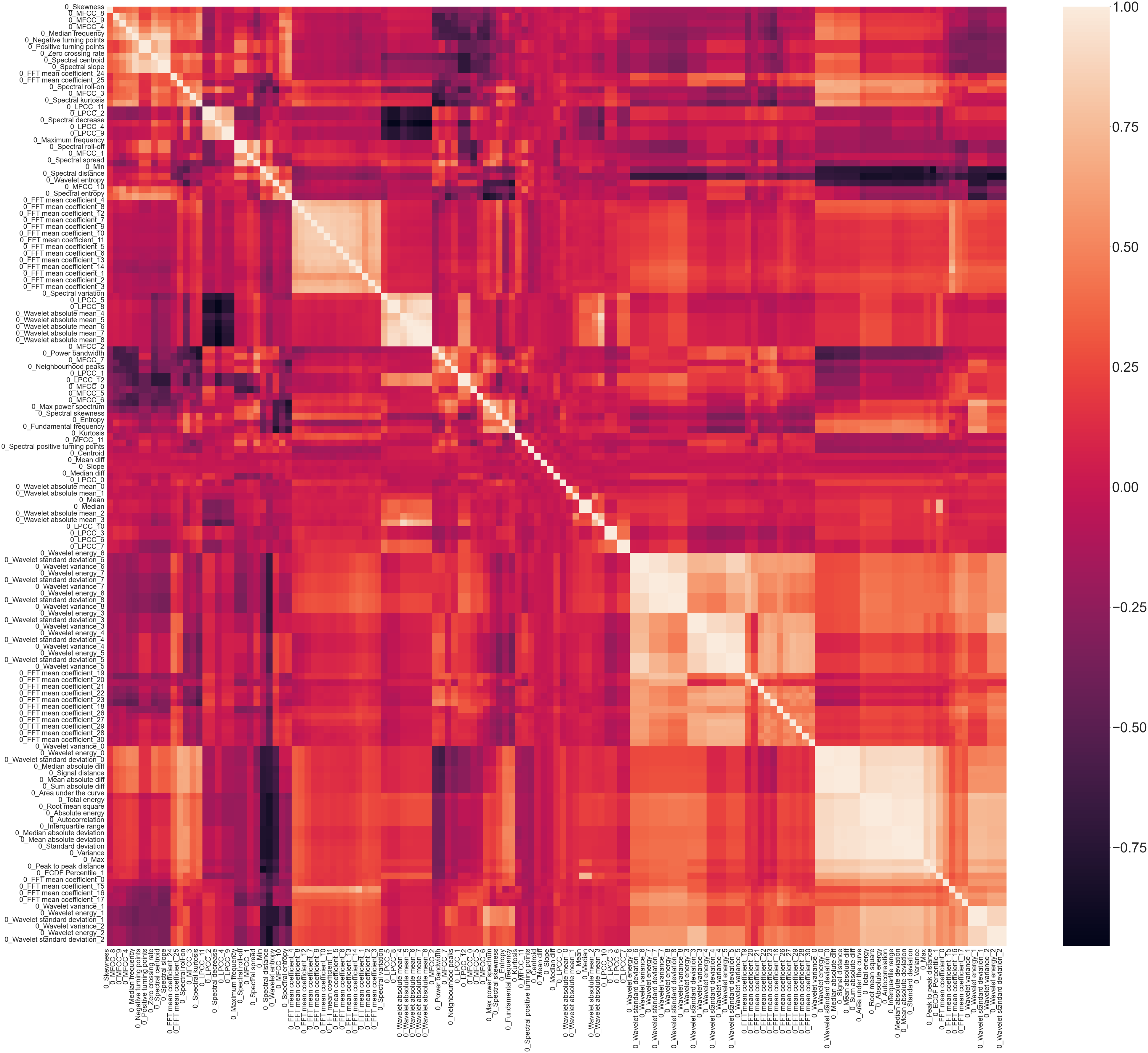
To reduce the number of features and the presence of multicollinearity in the dataset, hierarchical clustering is applied to the spearman rank-order correlations shown in Figure 19. A dendrogram, Figure 20, provides a visual representation of the hierarchical clusters for the feature set from the Z24 PDT FVT dataset. Dendrogram of hierarchical clustering of features, Z24 PDT FVT dataset.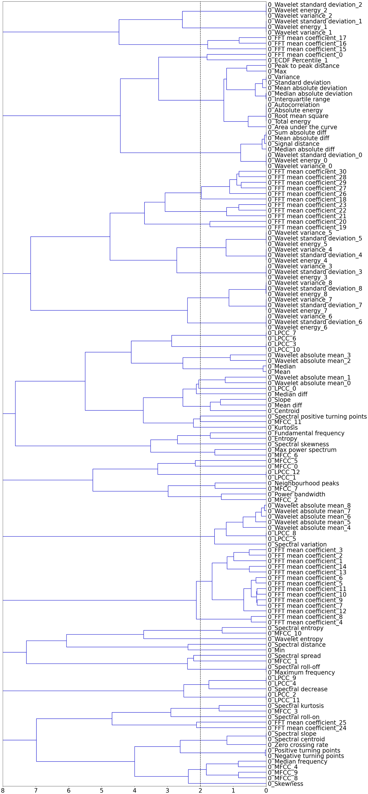
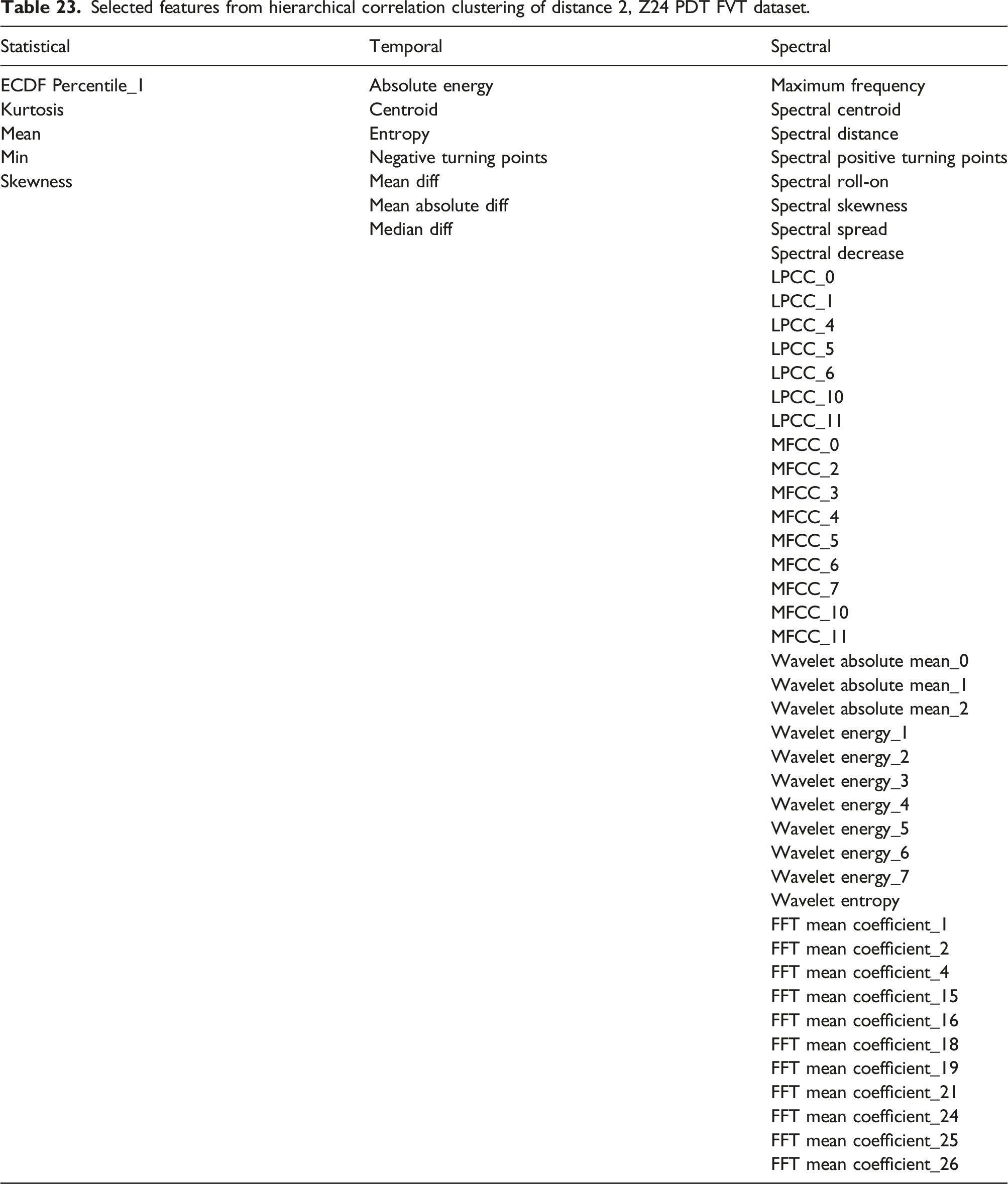
The x-axis of the dendrogram shows the distance between each of the clusters. The number of clusters decreases with increase in clustering distance. To reduce the correlated feature set, a threshold is set along the x-axis of the dendrogram, and one feature is chosen from each cluster. Figure 21 shows how the performance of the classifiers varies with increasing hierarchical clustering distance thresholds (Table 23). Varying F1 score for each classifier with increasing cluster distance thresholds, Z24 PDT FVT Dataset. Selected features from hierarchical correlation clustering of distance 2, Z24 PDT FVT dataset.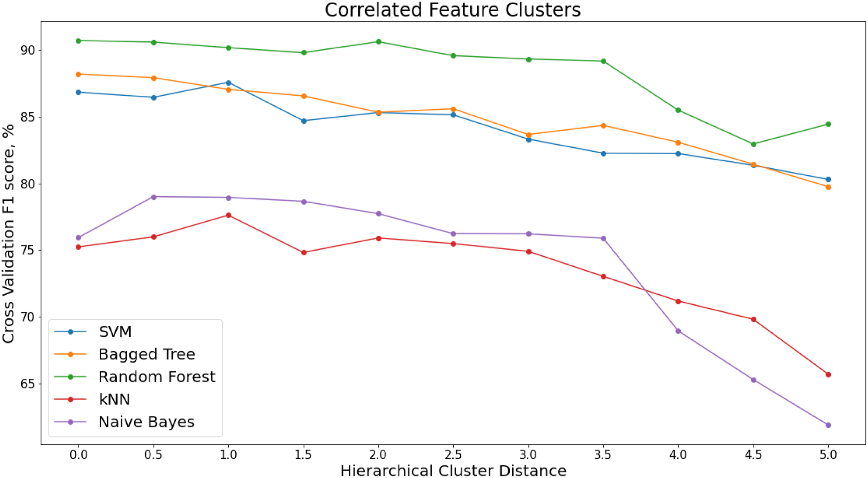
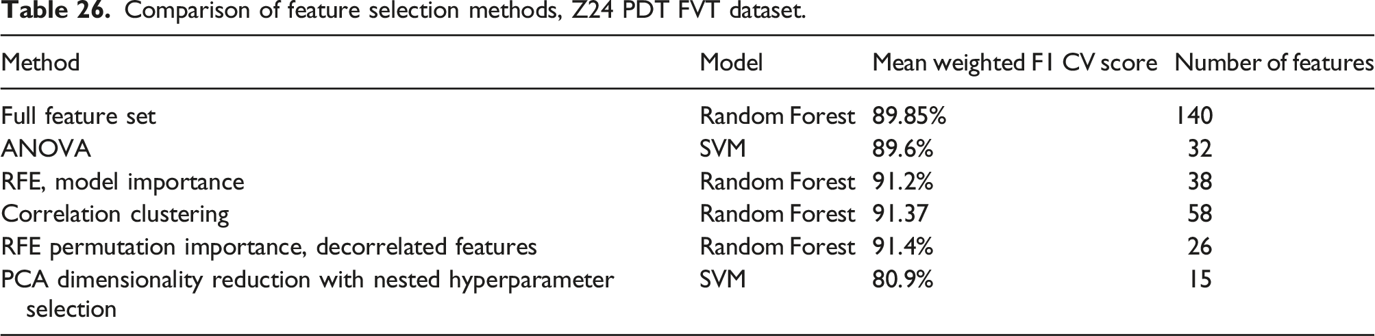
The highest F1 score is for the Random Forest model with a corresponding cluster distance of two. This results in and F1 score of 91.37% and a feature set of 58 features.
RFE with Permutation Importance
When features are collinear, permuting one feature will not have much effect on the model prediction performance as the same information can be obtained by the model from a correlated feature. RFE with Permutation importance is therefore applied to the decorrelated feature set presented in. The variation in F1 score with different percentages of permuted features from across the cross-validation folds is shown in Figure 22 for the decorrelated dataset from the hierarchical clustering. Recursive Feature Elimination (RFE) for varying percentiles of decorrelated feature set, ranked by permutation importance, Z24 PDT FVT dataset.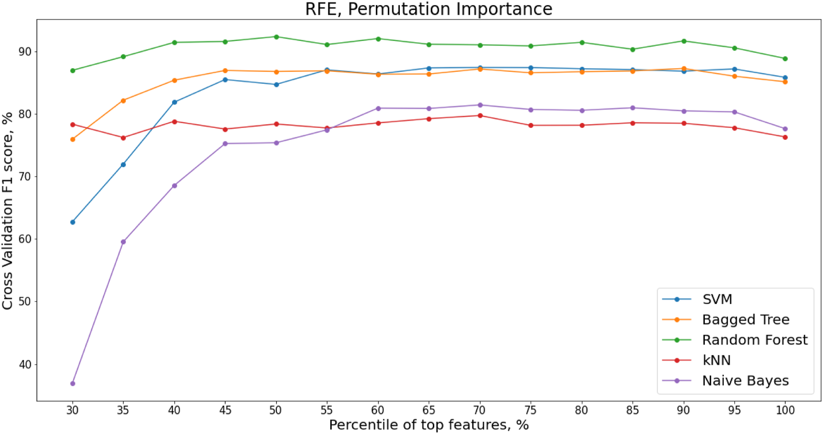
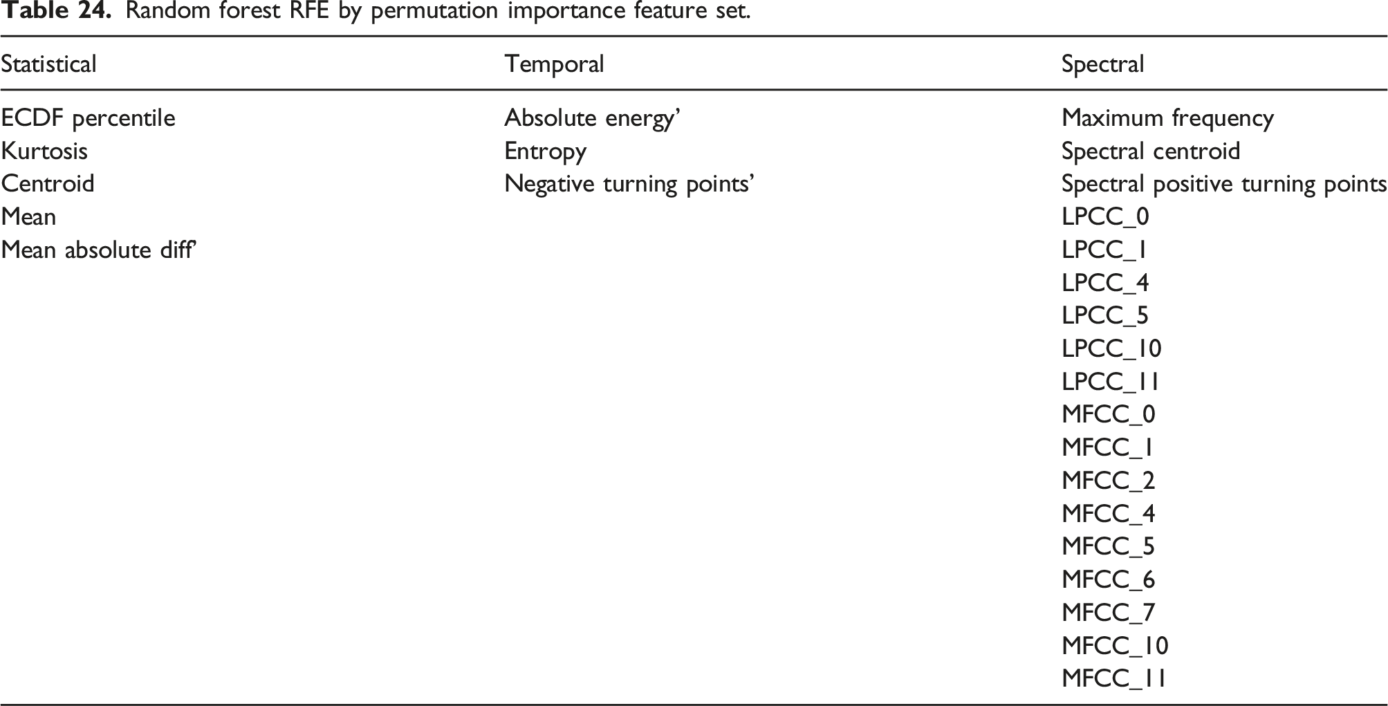
Random forest RFE by permutation importance feature set.
PCA Benchmark
The feature set of statistical time domain, temporal time domain and spectral time-frequency domain features is transformed using PCA before being used as the input features to each of the classification algorithms.
The same 5-fold stratified cross-validation procedure is used to train and test the classification model on the transformed feature set and the number of principle components are chosen to model 90% of the variance within the training dataset.
Classification performance with principal component transformation, Z24 FVT PDT dataset, nested cross-validation hyperparameter selection.
Comparison of Feature Subsets
Comparison of feature selection methods, Z24 PDT FVT dataset.
Discussion
The work outlines an approach to determining which is the minimum set features that best distinguishes between Healthy and damaged states in bridges. In order to determine this feature set, a supervised classification approach is implemented on two datasets where full scale bridges were subjected to progressive damage. 140 statistical time domain, temporal time domain and spectral time-frequency domain features are extracted from both datasets. The entire feature set is first used to test the ability of classification models to distinguish between the damage states using the extracted feature set. In order to reduce model overfitting and due to the sequential nature of the data, a 5-fold stratified cross validation approach is taken for the training and testing of each classifier. Four different feature selection methods are then applied to the feature set to obtain a minimum feature set that has comparable classification prediction performance to the entire feature set. The datasets used are the benchmark S101 and Z24 bridge datasets. As it is a combination of precision and recall, the F1 score was used as an evaluation metric for each of the feature selection methods.
The S101 dataset includes continuous recording of acceleration data over a number of days as the bridge is subjected to various damage events. The bridge vibrations come from traffic passing below the bridge and from the damage events that the bridge is subjected to. One of the challenges with the S101 dataset is that the length of each damage sequence varies significantly which results in an imbalanced dataset. An unshuffled stratified sampling is used for obtaining the training and test sets for each cross-validation fold. Although this maintains the time sequence in the dataset, the models sometimes struggled to accurately distinguish between preceding or proceeding damage states when the stratified test set was taken from the boundary of the damage classes, One of the challenges with classifying damage states is that the output of the classification model is the final decision. The confidence the model had in each classification prediction or the probability of a data point belonging to a specific state is not shown. With many different classes, the classification model might not be able to exactly predict the right class. The separation between classes is based on observations that are somewhat arbitrary. Although each class contains data from a unique damage event, damage effects may have occurred gradually, or there may be some delay between class boundaries and the start of the next damage event.
From the Z24 dataset, the recordings from the progressive damage tests are used in this analysis. Data was recorded for ambient vibration, with the only excitation coming from traffic passing below the bridge, and from forced vibration tests where a shaker was installed on the structure. In the S101 dataset, the sensors are recording while the damage event is taking place. For the Z24 PDT dataset, nine separate measurements of 1 h are taken for the bridge in each damage state, but the recordings do not include the actual damage events. Based on the classification performance it is observed that the features offer no ability to distinguish between the damage states with a lack of any meaningful vibrations in the system. In contrast, the classification prediction performance from the forced vibration tests is very high. The FVT data was therefore used for the Z24 feature selection analysis.
From comparisons of the feature selection methods for the S101 and Z24 PDT FVT datasets, respectively, the reduced feature sets obtained using the feature selection methods compare favourably in the obtained F1 score to the classification using the full feature set. The recursive feature elimination methods, using model importance and permutation importance tend to have a higher F1 score for a lower number of features than the ANOVA filter method and the features obtained through correlation clustering. This is expected as ANOVA filtering and correlation clustering are implemented independently of the classification models. The ANOVA filtering method is only related to how each individual feature varies across the different damage states and the clustering method is independent of both the damage states and the models and is implemented in an unsupervised manner. The RFE model importance shows the importance of features in the training of the model and the permutation importance shows the importance of features to the classification predictions. The most important class in terms of confidence of prediction is the healthy class versus the damage classes. For both the S101 and Z24 datasets, a high classification performance is achieved for distinguishing between the healthy state and the damage states.
For both the S101 and Z24 PDT FVT datasets, the tree-based methods, Random Forest and Bagged Tree, generally have the highest classification performance across different feature combinations and subsets. One of the challenges with this dataset is the similarity between classes. The bagging in both Random Forest and Bagged Tree and the random subspace method in Random Forest prevents overfitting, leading to better classification performance on the unseen test datasets.
The k-NN and Naïve Bayes methods had consistently poor classification prediction performance in distinguishing between each of the structural states. The poor classification performance of the k-NN model is due to the model not being able to create meaningful boundaries that adequately separate each of the damage states. This is likely due to the similarity in the data between classes leading to the lack of a clear structure between classes, particularly on the boundaries between damage states. The Naïve Bayes model assumes that feature values are statistically independent within each class 66 and for a Gaussian Naïve Bayes it is assumed that the continuous values within each class are normally distributed. It is likely that the poor classification performance is due to these assumptions not being met in the dataset. Alternatively, tree-based methods do not make any assumptions about the distribution of the data.
For the S101 dataset, there is a significant difference between the number of features chosen using Recursive Feature Elimination (RFE) versus the other feature selection methods for similar classification performance. The ANOVA and correlation clustering methods of feature selection do not factor in the classification performance when eliminating features. Alternatively, the RFE is a greedy method which recursively ranks and refits the model for each feature combination. The RFE is therefore often a more efficient method for obtaining the minimum feature subset that maximises classification performance. For the Z24 PDT FVT dataset, Table 5.10, the RFE method using model importance has a higher number of features than the ANOVA filtering method; however, the classification performance is higher.
From the output tables in the analysis of the S101 and Z24 PDT FVT datasets, the features chosen by each feature selection method varies. Features from each of the statistical time domain, temporal time domain and spectral time-frequency domain feature types are selected by each method with the spectral time-frequency domain features dominating as the most important for classification prediction performance. In the context of remote wireless SHM, the challenge with spectral time-frequency methods is that they are more computationally expensive.
There is no consistent set of features which are deemed most important to each feature selection approach to distinguish between the damage classes. There are several reasons for this variation in the chosen feature sets. There is a significant amount of noise in both the data and the class labels and the low classification accuracy for the cross-validation folds at the boundaries of the classes demonstrate this. Secondly, as they are extracted from the same acceleration signal, there is a lot of similarity in the information captured by many of the features, particularly the between time domain and time-frequency domain categories. Although there are a number of other time-frequency methods also available, such as HHT 40 and EEMD, 43 these methods are even more computationally expensive and unlikely to add any further damage sensitive information that has not already been captured in the signal. Finally, each of the feature selection and machine learning model combinations vary significantly in the manner in which they reduce the feature sets.
To benchmark the classification performance of each of the reduced feature sets, PCA is applied to reduce the dimensionality of the feature set. As this transformation removes the original relationship between the features and each of the damaged classes, it is necessary to reselect the model hyperparameters. To avoid biasing the model performance as nested cross validation procedure is applied, as shown in Tables 4.10 and 5.10. The classification performance from the models trained using the principle components are less than each of the models trained using the selected feature sets. Despite the nested cross validation approach to hyperparameter selection, it is evident that much of the relationship between the features and the classes is lost due to the transformation of the features using PCA.
Rather than taking the principal components of the entire feature set, a recommendation for future research work would be to individually apply PCA to each of the multi-dimensional feature types (such as the spectral feature outputs from each of the spectral feature extraction methods). This could help reduce the dimensionality of the feature vectors before any feature selection methods are applied, while maintaining the relationship between the feature sets and the multi-class damage states.
Conclusion
A baseline of univariate features, supervised classification models and feature selection methods for identifying the minimum set of features which in combination are most effective for detecting damage in bridges is presented. Data from two benchmark full scale bridges are used in this analysis which contain acceleration recordings from measured progressive damage tests. It is shown that combinations of statistical time domain, temporal time domain and spectral time-frequency domain features achieve a higher performance in distinguishing between damage states than the use of individual features or the full set of features. This work shows that features extracted from univariate, single sensor, acceleration signals can accurately distinguish between multiple damage states in full scale structures. Using various feature selection methods, subsets of these features are obtained which achieve similar classification performance of damage states to the entire feature set.
If an SHM campaign is being implemented on an operational bridge, it is not feasible to first train a model with labelled damage scenarios from that structure. Although attempts have been made in this regard with finite element models and Deep transfer learning, it is not possible to quantify the damage a structure may undergo in the future. Therefore, the implementation of a SHM system requires an unsupervised or novelty detection approach. As the feature subsets obtained in this analysis have shown to be effective in distinguishing between damage states with supervised learning, the next step is to use these feature subsets as inputs into an unsupervised model for identifying damage as it occurs. Hierarchical clustering has been shown to be an effective means of reducing the feature set without much loss in classification prediction performance by removing correlated features. As opposed to the other feature selection methods presented in this work, the reduction of the feature set using hierarchical clustering is based on feature correlations and requires no knowledge of the damage classes. Therefore, this method would be suitable for feature set reduction in an unsupervised SHM approach.
For the reproducibility of the results presented, the code base and extracted feature data has been made available at https://github.com/tadhg-buckley/Feature-Extraction-Selection-Benchmark-SHM. Although the raw data cannot be publicly made available, the extracted feature datasets are included so that the outputs can be easily reproduced and other classification and feature selection methods can be applied.
Footnotes
Acknowledgements
Bidisha Ghosh would like to acknowledge SFI Centre CONNECT. For the purposes of Open Access, the authors have applied a CC BY public copyright licence to any Author Accepted Manuscript version arising from this submission.
Declaration of Conflicting Interests
The author(s) declared no potential conflicts of interest with respect to the research, authorship, and/or publication of this article.
Funding
The author(s) disclosed receipt of the following financial support for the research, authorship, and/or publication of this article: The authors acknowledge funding from Science Foundation Ireland (SFI) under Grant number 12/RC/2302_2. VP acknowledges the support of the EU-funded SIRMA project (Strengthening Infrastructure Risk Management in the Atlantic Area–Grant No. EAPA/_826/2018).
Appendix
The features extracted from the acceleration signals are summarised in Table 27.
Univariate features.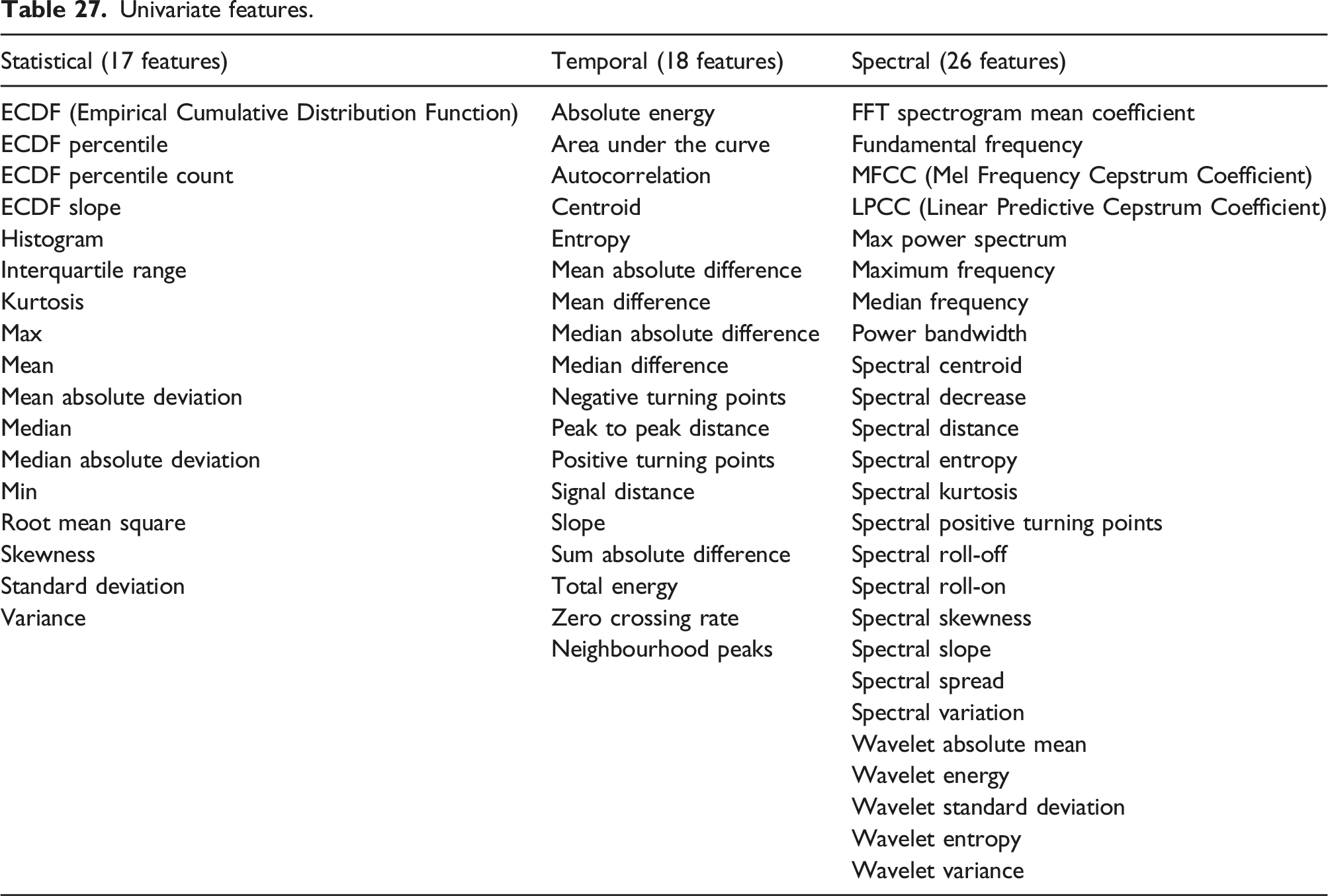
Statistical (17 features)
Temporal (18 features)
Spectral (26 features)
ECDF (Empirical Cumulative Distribution Function)
Absolute energy
FFT spectrogram mean coefficient
ECDF percentile
Area under the curve
Fundamental frequency
ECDF percentile count
Autocorrelation
MFCC (Mel Frequency Cepstrum Coefficient)
ECDF slope
Centroid
LPCC (Linear Predictive Cepstrum Coefficient)
Histogram
Entropy
Max power spectrum
Interquartile range
Mean absolute difference
Maximum frequency
Kurtosis
Mean difference
Median frequency
Max
Median absolute difference
Power bandwidth
Mean
Median difference
Spectral centroid
Mean absolute deviation
Negative turning points
Spectral decrease
Median
Peak to peak distance
Spectral distance
Median absolute deviation
Positive turning points
Spectral entropy
Min
Signal distance
Spectral kurtosis
Root mean square
Slope
Spectral positive turning points
Skewness
Sum absolute difference
Spectral roll-off
Standard deviation
Total energy
Spectral roll-on
Variance
Zero crossing rate
Spectral skewness
Neighbourhood peaks
Spectral slope
Spectral spread
Spectral variation
Wavelet absolute mean
Wavelet energy
Wavelet standard deviation
Wavelet entropy
Wavelet variance