
Abstract
Failure of pipe network components in so-called mixing zones due to high-cycle thermal fatigue (HCTF) can occur within nuclear power plants where fluids of different thermal and hydraulic properties interact. Given that the consequences of such failures are potentially deadly, a method to monitor HCTF non-invasively in real-time is expected to be of great use. This method may be realised by a technique to determine the inaccessible temperature distribution of a component since thermal gradients drive HCTF. Previous work showed that a physics-based method called the inverse thermal modelling (ITM) method can obtain the temperature distribution from external temperature and ultrasonic time of flight (TOF) measurements. This study investigated whether the long-short-term memory (LSTM) machine learning architecture could be a faster alternative to the ITM method for data inversion. On experimental data, a 25-member ensemble of LSTM networks achieved an ensemble median root mean square error (RMSE) of 1.04°C and an ensemble median mean error of 0.194°C (both relative to a resistance temperature device measurement). These values are similar to the ITM method which achieved a RMSE of 1.04°C and a mean error of 0.196°C. The single LSTM network and the ITM method achieved a computation-to-real-world time ratio of 0.008% and 14%, respectively demonstrating that both methods can invert data in real-time. Simulation studies revealed that LSTM performance is sensitive to small differences between the training and real-world parameters leading to unacceptable errors. However, these errors can be detected via an ensemble of independent networks and, corrected by simply adding a correction factor to the TOF prior to being input into the networks. The results show that LSTM has the potential to be an alternative to the ITM method; however, the authors favour ITM for temperature distribution monitoring given its interpretability.
Introduction
Motivations
Pipe networks within nuclear power plants (NPPs) are susceptible to high-cycle thermal fatigue (HCTF) in so-called mixing zones where fluids of different thermal and hydraulic properties interact.1,2 This susceptibility is, in part, due to the high thermal expansion coefficient and low thermal conductivity of austenitic stainless steels (SSs) 3 that are used throughout different types of NPPs.4,5
In May 1998, a crack of a pipe elbow within the reactor heat removal system (RHRS) caused a leak at the French Civaux 1 pressurised water reactor after just 1500 h of operation. 6 The leak caused the release of radioactive steam at a rate of 30 m3 h−1 into the reactor building. 7 The location of the 180 mm through-wall crack on the pipe elbow is shown in Figure 1. Following this incident, Civaux 1 and three other reactors of the same design were defueled, and a failure analysis was performed. 7 The analysis identified that the failure was caused by thermal-fatigue-initiated cracks. 8 This HCTF phenomenon had not been considered during the design of the NPPs since it was not captured in the design standards of the time. 6 Hence, redesign, requalification and replacement of the affected components of the RHRS in all four reactors had to be performed. Subsequent ultrasonic inspection in 1999 of all NPPs in France revealed that thermal fatigue cracking was not unique to the Civaux 1 reactor design (due to the limitations of the design standards 6 ). Further research identified that mixing zone HCTF is primarily caused by repeated exposure to temperature fluctuations affected by differences >50°C between hot and cold fluids. 6 It was also found that the fatigue is most severe for temperature fluctuations with frequencies in the range from 0.1 to 1 Hz.9,10
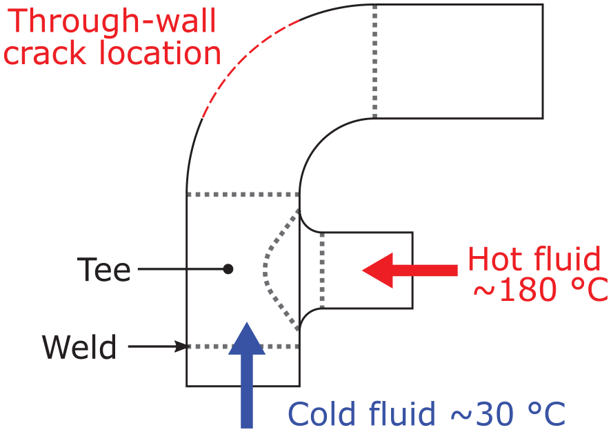
Schematic of the Civaux 1 RHRS pipe elbow illustrating the location of the fatigue crack location.
Given the susceptibility of austenitic steels to thermal fatigue, 3 and that safety is paramount in the nuclear industry, it is desirable to investigate techniques that can monitor the progression of HCTF and as a result, relax the requirements on the inspection interval and remove operators from the hazardous environment.
Article structure
The remainder of the article is structured as follows: the section ‘Limitations of current HCTF monitoring methods’ details the short-comings of current HCTF monitoring methods, and the physical reasons for this. A brief explanation of a physics-based ultrasonic temperature inversion method is presented in the section ‘Inverse thermal modelling method’. The section ‘Long short-term memory’ describes the machine learning network architecture considered in this work, the process for generating (simulated) training and testing data and the steps for training networks. The section ‘Simulation studies’ defines an initial test case and two additional test cases concerning data that have never been seen before seen by the trained networks. The section ‘Experimental studies’ introduces experimental data used to evaluate the machine learning networks on real-world data. The results of the machine learning networks are shown and discussed first for the simulated test data followed by the experimental test data, with results for the physics-based inversion method included for comparison. Finally, a summary of the key findings are provided in the conclusions.
Limitations of current HCTF monitoring methods
A component exposed to temperature fluctuations will develop thermal gradients that will generate thermal stresses. If sufficiently large, these stresses will impart damage leading to crack initiation/propagation and eventually cause the component failure. This failure mechanism is known as thermal fatigue. 11 For a pipe carrying a thermally varying fluid, the inaccessible interior surface will experience the largest (compressive or tensile) stresses.
Since thermal fatigue progression is driven by thermal gradients, knowing how the through-thickness temperature profile evolves over time is vital for monitoring thermal fatigue. 10 However, this is a difficult task because traditional temperature measurement equipment (e.g. thermocouples) can only measure surface temperatures. Several techniques to overcome this issue have been developed; the following two sections will introduce and evaluate these techniques.
Embedded thermocouples
The obvious method to obtain the temperature profile in a component is by embedding sensors into a component. This method is demonstrated in two studies12,13 by embedding thermocouples throughout the thickness of a component via drilled holes. However, these holes will create stress-raising features that will accelerate thermal fatigue progression. 14 Furthermore, RTDs resistance temperature detector have been shown to lag true temperature in the order of seconds due to thermal conduction into the device 15 causing measurement errors.
FAMOSi
The integrated FAtigue MOnitoring System (FAMOSi) was developed by Siemens in the 1980s and later updated by Areva (a French multinational group with a focus on nuclear power) for thermal fatigue monitoring following the discovery of fatigue cracks in NPPs. 16 The resulting non-invasive system, called Integrated FAMOS (FAMOSi), comprises seven temperature sensors mounted around one half of a pipe’s circumference as shown in Figure 2. The system is based on a comparison of the outer surface temperature-time history to a pre-compiled reference database of ‘responses’ which are computed via a finite element model (FEM). It is likely to be a significant task to validate the FEM. Furthermore, the system is incapable of detecting thermal fluctuations >1 Hz. 17 Although the reason for this limitation is not explicitly stated in the literature, it is assumed to be due to the low thermal conductivity of austenitic steels preventing thermal energy from diffusing to the component’s outer surface rather than a limitation in computational or data acquisition capabilities. This effect is demonstrated in the next section.
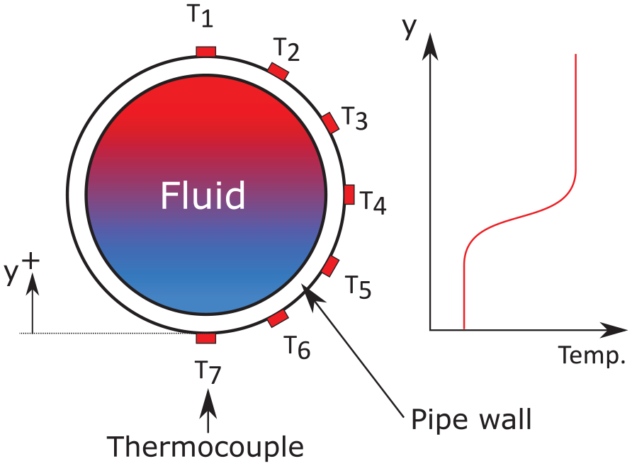
Schematic diagram of FAMOSi.
Thermal conduction: a low-pass filter
This section presents simulations to demonstrate that materials with low thermal conductivity effectively act as low-pass filters of temperature. This low-pass effect implies that the previously introduced HCTF monitoring methods, based on externally mounted temperature sensors, will be unsuitable for resolving sub-surface temperatures that fluctuate rapidly, especially for thick components.
An explicit 1D, finite difference heat transfer model with convective boundary conditions was developed based on the model used by Zhang et al.
18
The model simulated the temperature profile evolution of a section of 304 SS pipe carrying water at constant pressure and the outer surface exposed to air as shown in Figure 3. The fluctuation frequency of the water temperature was set to be a linear up-chirp: the instantaneous frequency increases linearly with time. The properties and parameters of the simulation are summarised in Table 1 where T, h, k,
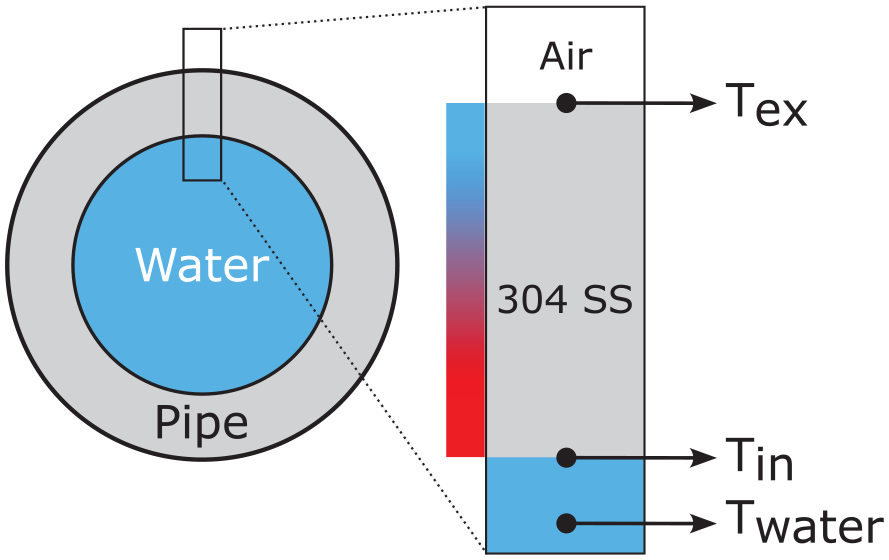
Schematic of the simulation setup. The colour bar denotes an arbitrary temperature gradient due to the difference in temperature between the air and water.
Parameters and material properties used in the simulation (304 SS).
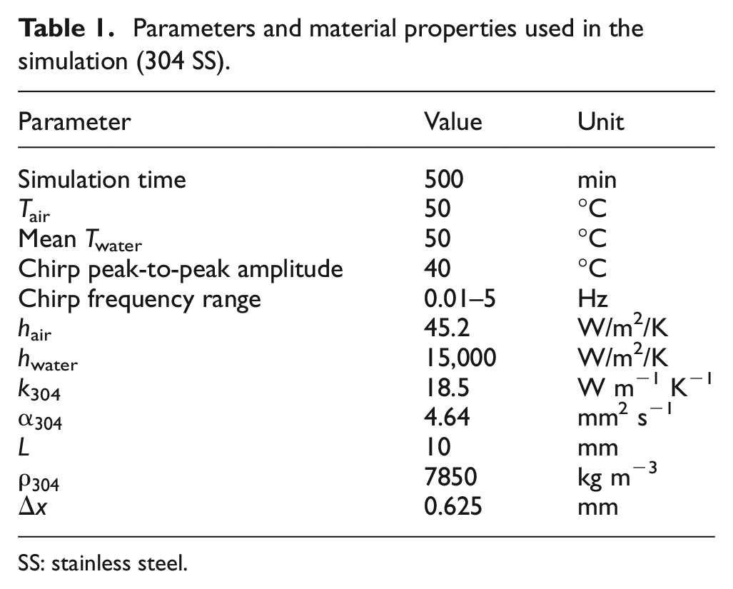
SS: stainless steel.
The 500 min of simulated time yields a rate of change of chirp frequency of
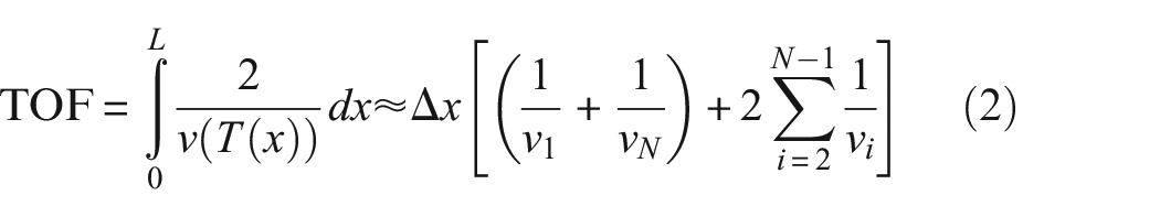
In Equation (2)

Figure 4 shows the water temperature
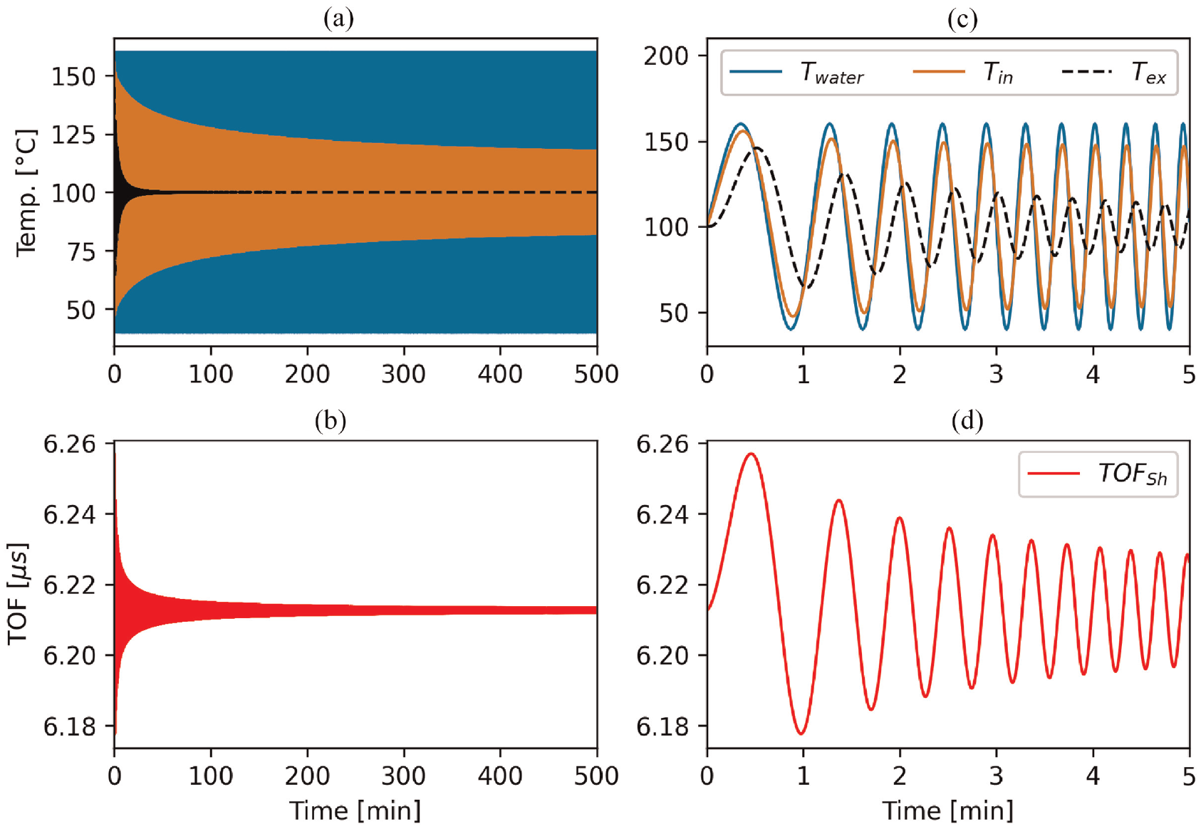
Results of the finite difference simulation for a 10 mm block of 304 SS exposed to temperature-varying water that fluctuates according to a sine wave with linearly increasing frequency. Temperatures of the water, and at the inner and outer surface of the component are shown in the top row. The bottom row shows the shear TOF. Panels (c) and (d) are zoomed to show the first 5 mins of panels (a) and (b), respectively. The left column shows full 500 min of the finite difference simulation whilst the plots in the right column show only 5 min.
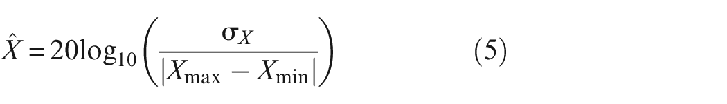
A spectrogram of the full 500 min of simulation for each variable is shown Figure 5. The horizontal lines at 0.1 Hz (red dash-dot) and 1 Hz (white dashed) are superimposed on Figure 5 to show the range of critical fluctuation frequencies for HCTF of the tee-joint at Civaux.9,10 The spectrograms were computed to identify the maximum resolvable fluctuation frequency for each variable. To create a spectrogram, a given variable was segmented into periods of 2048 time steps. The Fourier transform was computed for each period and stacked along the x-axis, that is, a visual representation of the frequency content of a signal for each consecutive 2048 time step period. Each variable was normalised by its absolute range before the spectrogram was computed, that is, Equation (4).
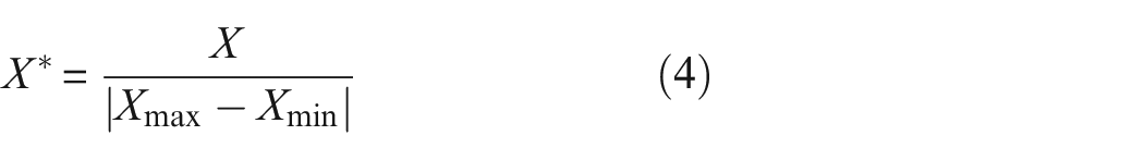
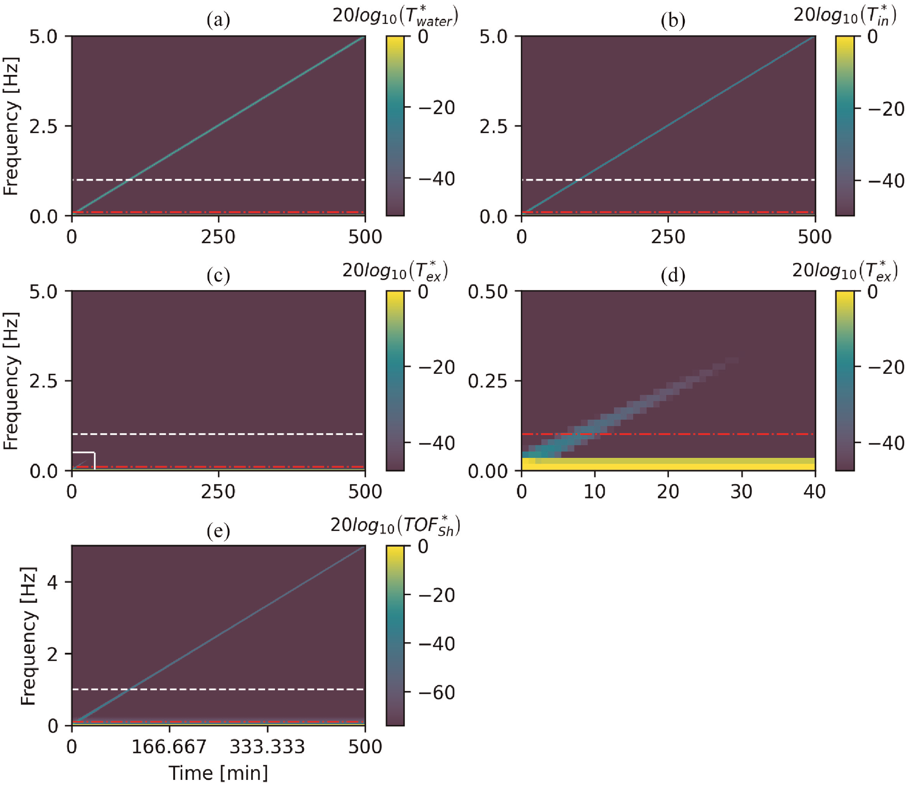
Spectrograms for the temperatures (a)–(d) and, shear TOF (e) computed by the finite difference simulation (Figure 4). Each variable was normalised according to Equation (4) before computing the spectrogram. The horizontal red dash-dot and white dashed lines denote 0.1 and 1, respectively. The solid white lines in panel (c) bound the zoom extents for panel (d).
The minimum of the colour bar
For temperature,
Figure 5(d) shows that a temperature sensor mounted to the external surface of a component cannot differentiate temperature fluctuation frequencies greater than approximately 0.29 Hz. Furthermore, the practical frequency limit is likely lower than 0.29 Hz due to the lag time of typical temperature sensors15,18,23 which is not considered in these simulations. In contrast, the shear TOFs (Figure 5(e)) remain sensitive up to 5 Hz. TOF should remain sensitive well beyond 5 Hz although the theoretical upper limit of the sensitivity was not investigated in this simulation. The upper limit is expected to be governed by the sampling rate of the acquisition hardware.
Inverse thermal modelling method
A feasibility study by Zhang et al. 18 utilised the thermal sensitivity of (shear) ultrasonic TOF (as shown in the previous section), demonstrating internal surface temperature estimation within 2°C. The method couples TOF and outer (accessible) surface temperature measurements with a physics-based inversion model to obtain temperature estimations. Of the two inversion methods presented by Zhang et al., only the inverse thermal modelling (ITM) method based on earlier work by Ihara et al. 24 will be considered in this article.
The ITM method is based on iterative optimisation of an explicit finite difference formulation of the inverse heat conduction problem enabling it to obtain the full temperature profile. The explicit formulation requires that the time step of the data must be sufficiently small to ensure a stable solution. Hence, interpolation of the data is usually necessary to ensure stability which increases computational expense.
Long short-term memory
Machine learning is a technique that is being increasingly implemented in non-destructive evaluation scenarios, including:
Ultrasonic flaw classification 25
Deconvolution of ultrasonic signals 26
Artefact identification and suppression in ultrasonic images 27
Defect detection in guided wave signals 28
Noise quantification in ultrasonic images 29
Ultrasonic crack characterisation 30
Machine learning has several beneficial characteristics including:
A physics-based model of an underlying system is not required 31
The ability to implicitly create complex non-linear relationships
One drawback is that it is difficult to explore the explainability of the mathematical operations inside the model leading to machine learning networks to often be described as a ‘black box’ method. 32 Very broadly, deep learning – a subset of machine learning – can use all the available information embedded within the data set by simply using the raw data as the input. In contrast, shallow learning requires hand selection of input features but requires less training data than deep learning. 33 Within deep learning, recurrent neural networks (RNNs) are well suited for problems involving time-series data; however, they can be susceptible to gradient vanishing and gradient exploding problems. 34 To overcome this issue, a novel and efficient gradient-based method, called long short-term memory (LSTM) was developed by Hochreiter and Schmidhuber. 35 This article explores whether machine learning networks can replace the (single shear wave) ITM inversion method for real-time temperature gradient monitoring using networks trained using simulation data only. Given the available scope of this article, it would not be possible to explore all potential machine learning architectures. The LSTM architecture was selected for investigation as it seemed a prominent candidate and showed promising results in initial evaluations. For a detailed discussion of other types of architectures that have been proposed for a range of non-destructive evaluations applications, beyond time-series data, the review paper by Cantero-Chinchilla et al. 36 is suggested to the interested reader.
Figure 6 shows a schematic of an LSTM cell that contains four layers. The four layers comprise three logistic sigmoid and one hyperbolic tangent (tanh) functions that interact to produce the output and the state of the cell which are then passed onto the next hidden layer. An LSTM cell has three inputs:
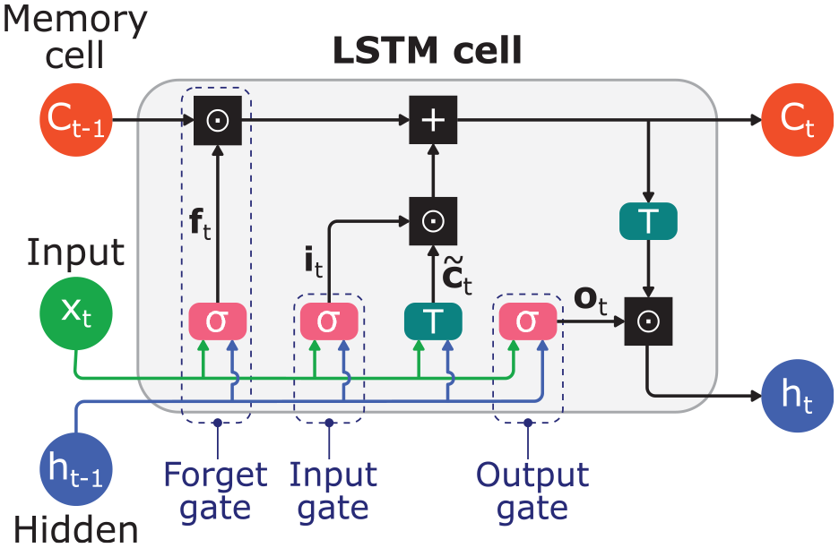
Graphical illustration of an LSTM cell. The weights are omitted for clarity.
Train/test data generation and network training
The previously introduced finite difference heat transfer code was used to generate data sets for training and testing LSTM networks. However, the method for defining the water temperature fluctuations differed. The first method (later referred to as the sine method) defined the fluctuations to be sinusoidal (rather than a linear chirp) and were defined by three parameters:
1. Mean temperature (increasing, decreasing, or constant)
2. Temperature range (increasing, decreasing, or constant)
3. Fluctuation frequency (
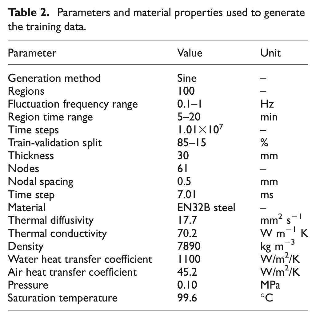
Each of the parameters was selected for each ‘region’ in the data set using uniform random distributions; discrete forms of the distribution are used for the mean temperature and temperature range. Figure 7 shows nine representative regions demonstrating each of the possible mean temperature and temperature range combinations for the sine method. The training data set used to train all LSTM networks was generated using the parameters given in Table 2.
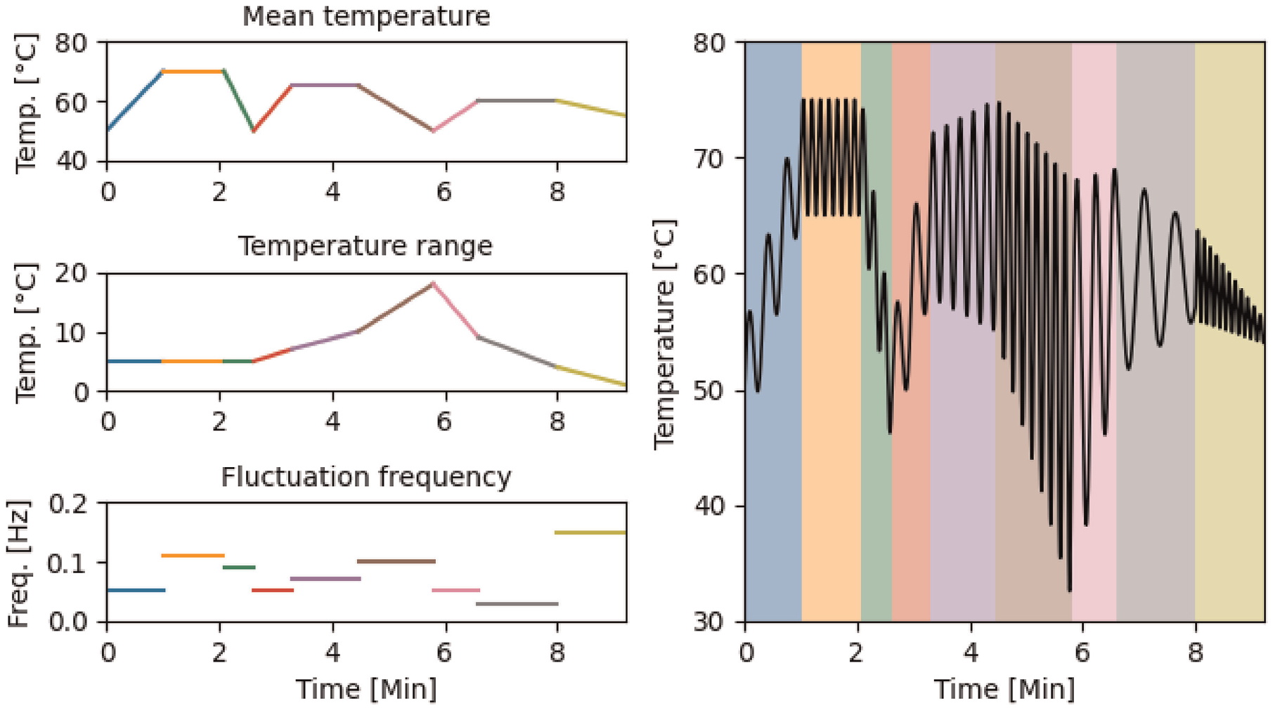
Representative example showing a region for each of the possible nine mean temperature and temperature range combinations used when generating
Parameters and material properties used to generate the training data.
The second method (later referred to as the square method) used to create a test set that mimics the experimental data introduced in a later section, defined the fluctuations as square waves. In both methods, the upper limit of
The networks were created in Python 3
40
using the Keras deep learning API.
41
Each network comprised a single LSTM layer with 180 neurons followed by a one-unit dense layer. An 85:15 train-validation split was used on training data sets, and separate unseen data sets were used for testing. All training sets were generated using the sine method. The input data were assembled such that for a given time step, the data passed to the network contained two values: the value at the current, and one previous time steps. The Adam optimiser
42
was used in conjunction with Equation (6) which describes the exponentially decaying learning rate,

The mean square error was used as the loss function. Early stopping based on 25 epochs without reduction of the validation set loss was used to prevent the networks from over-fitting to the training data. The networks were trained with a 12th Gen Intel core i7 processor CPU of a desktop PC. This PC was used throughout the work presented in this article.
A manual ‘trial and error’ approach was used over formal optimisation strategies of the LSTM networks for two reasons. Firstly, because this work set out to determine whether machine learning might be a less computationally expensive alternative to physics-based methods rather than finding the best (highest accuracy) machine learning method. Secondly, the first trial implementation yielded good results (single 50-neurons LSTM layer followed by a one-unit dense layer). Furthermore, better performance (defined as lower RMSE/mean error) should only be considered on experimental data. However, this poses a limitation due to the lag of RTDs15,18,23– the LSTM predictions are compared to a reference measurement rather than a ground truth during experiments. Hence lower RMSE/mean error on experimental data by LSTM would mean that the inherent lag of the RTDs is being learnt, this is not beneficial and hence a sensitivity study of changes in performance metrics was not attempted.
Simulation studies
It was expected that if a LSTM network could predict the temperature at a single distance from the water–metal interface, a more complex network would be able to predict the full temperature profile of a component. In this work, a single distance network was investigated to confirm whether the LSTM architecture was a suitable choice for data inversion. The single distance was chosen to be 5 mm from the water–metal interface to match the reference RTD distance in the experimental data (introduced later). A training set that simulated an EN32B mild steel block exposed to water on one side and the other exposed to constant temperature air was created using the sine method comprising 100 regions. A single shear wave was used since the changes in TOF were due to temperature changes only (the component thickness remained constant). The shear wave velocity–temperature relationship of the sample is given in Equation (7).

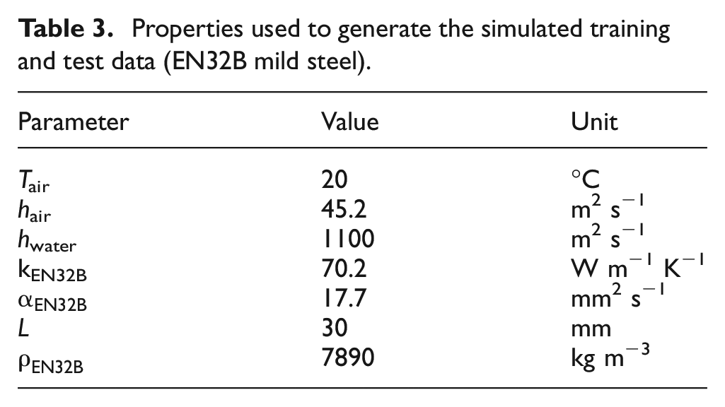
LSTM networks were then trained with this data set. Following training, the performance of the networks was evaluated using an initial simulated test set with the water temperature defined with the square method to switch between hot and cold, with the magnitudes and periods of exposure matching the experimental data set. The simulation parameters are shown in Table 3 where the symbols have the same definitions as in Table 1.
Properties used to generate the simulated training and test data (EN32B mild steel).
Deep ensemble
To observe the influence and minimise the impact of the random initialisation of the network weights each time a new network was trained, 100 networks (with identical architectures) were trained using the same training set. These networks were used to create a deep ensemble. Deep ensembles of machine learning networks have been shown to increase prediction accuracy and provide a measure of uncertainty.
33
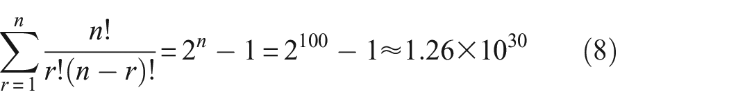
To determine a sufficient number of networks (members) in the ensemble, increasing numbers of members were included in the ensemble and the SD of the RMSE was computed. This process was repeated with random (unique) shuffles of the order in which the networks were included in the ensemble. However, only 20,000 shuffles were considered since for 100 networks it would be unrealistic to consider all
The range of the RMSE SD was compared to the (peak-to-peak) range tolerance, at the mean temperature of the simulated data set (

This comparison is shown in Figure 8. As expected, as the number of ensemble members reaches the maximum number, the range of the SD of the RMSE reduces to zero since a change in the inclusion order of networks becomes less significant. The ensemble SD range falls below that of the RTD after 10 members. While 10 members could be argued to be sufficient the authors decided to be conservative by including 25 members so that variations due to simulations would be smaller than those that are expected in experimental measurements. For the avoidance of any doubt, 25 of the 100 networks were randomly selected and the same 25 networks were subsequently used throughout this article for any and all simulation or experimental studies.
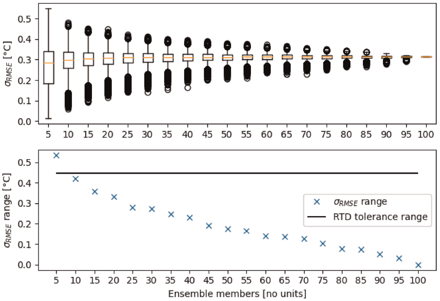
The upper panel shows the standard deviation of RMSE of the ensembles for increasing numbers of members in the LSTM ensemble for predictions on the baseline simulation test set. The standard deviations of the RMSE are shown for 20,000 unique random shuffles of the order in which networks are considered for inclusion in the ensemble. Values that were more than 1.5 × the interquartile range are shown by the circles. The lower panel shows the range of standard deviations of the RMSE (which are shown in the upper panel). In the lower panel, the solid black line denotes the tolerance range of a class A RTD 22 as defined by Equation (9).
Robustness against out-of-distribution data
Out-of-distribution data (OODD) are data that a trained network has never been exposed to because the training set does not capture it. The response of the LSTM ensemble to OODD was explored to assess two areas. Firstly, assess the magnitude of the impact of OODD on the ensemble, that is, how badly wrong do the predictions get on previously unseen data. Secondly, whether the deep ensemble could detect when the model is working outside of the predefined domain of operation using the SD of the ensemble predictions. The second area encompasses quantification of the epistemic uncertainty. Epistemic uncertainty arises from a lack of knowledge about data generation method, resulting in uncertain network parameters. The uncertainty can be reduced by increasing the amount of relevant training data, provided that the training data aligns closely with the test data. However, it is important to note that in this work the epistemic uncertainty cannot be fully eliminated because simulation data has been used to approximate real-world data leading to an inherent difference between training and test data. 33
Two independent OODD scenarios that were deemed most likely to occur in the real world were explored. The OODD scenarios were incorrect component thickness, and
Values of the velocity–temperature relationship coefficients used to generate the velocity OODD test sets. The percentage changes are relative to the values used when generating the base test set.
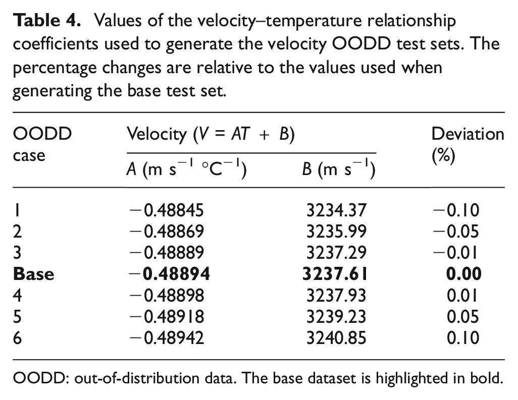
OODD: out-of-distribution data. The base dataset is highlighted in bold.
Values of the thicknesses used to generate the thickness OODD test sets. The percentage changes are relative to the values used to generate the base test set using absolute magnitudes.
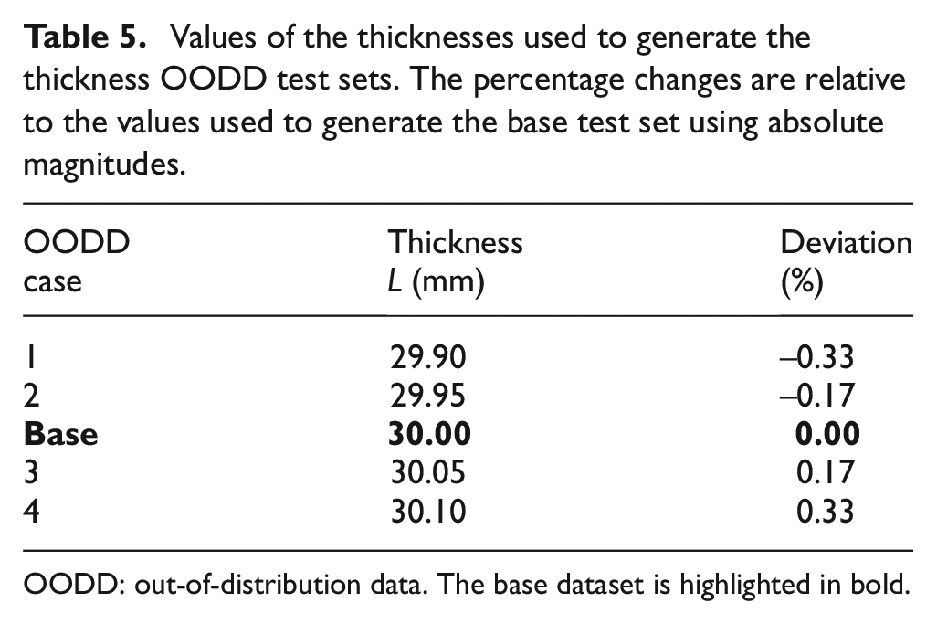
OODD: out-of-distribution data. The base dataset is highlighted in bold.
Experimental studies
The ‘temperature fluctuations only’ experiment data were provided by Zhang and Cegla
23
for use as a test set to evaluate the real-world performance of the 25 previously trained LSTM networks. The ITM MATLAB
43
code was also provided and then rewritten in Python. The experiment comprised a sample of EN32B mild steel
Prediction time
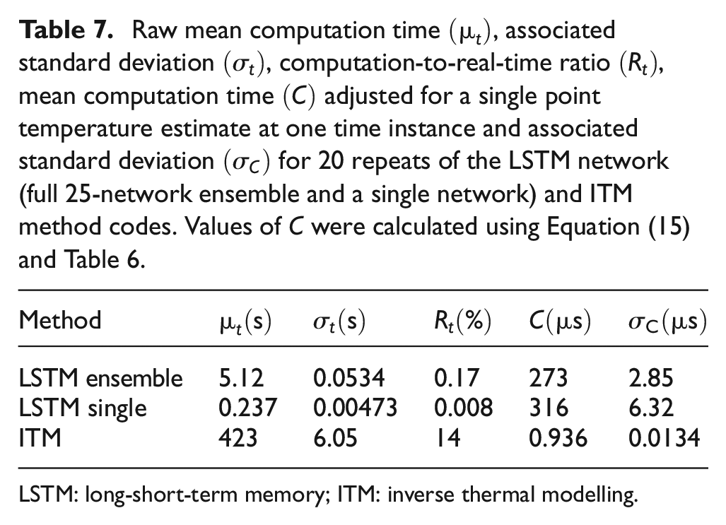
To investigate the computational time of the LSTM ensemble, single LSTM network and ITM method, their respective Python codes were run 20 times using the experimental test set. Their respective computation times were measured (using the perf_counter() function 44 ) and averaged. The snippets of code that were timed only included instructions explicitly related to making predictions.
Results and discussion
Throughout this section, Equation (10) was used to define the error between the true (simulated) or reference (RTD) measurement and the inversion method (LSTM or ITM) predictions whilst Equation (11) was used to define the error between the true (simulated) or reference (RTD) measurement and the external surface temperature. The subscript 5 mm refers to the distance from the water–metal interface that the simulated or experimental temperature measurements are taken from as the true and reference measurement, respectively.


Simulation studies
Figure 9 shows the results of the initial simulated test set. The top panel of Figure 9 shows the true (simulated) temperature 5 mm from the water–metal interface and the mean temperature predictions of the 25 LSTM networks at the same spatial location. One SD above and below the mean of the 25 networks is also superimposed to demonstrate the aforementioned impact of the random initialisation of each network. The bottom panel shows the error relative to the true temperature for the mean LSTM predictions as well as for the temperature at the steel block’s outer surface (the air–metal interface).
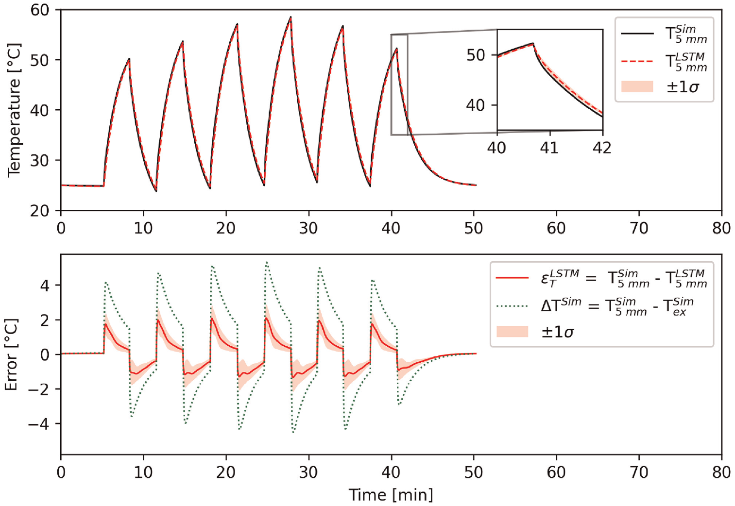
Initial simulated test set results. Top panel: simulated temperature 5 mm from the water–metal interface
Figure 10 shows the RMSE and mean error for the velocity OODD test sets taken over all time steps for each network. The metrics based on the external temperature are also shown as a reference. As both
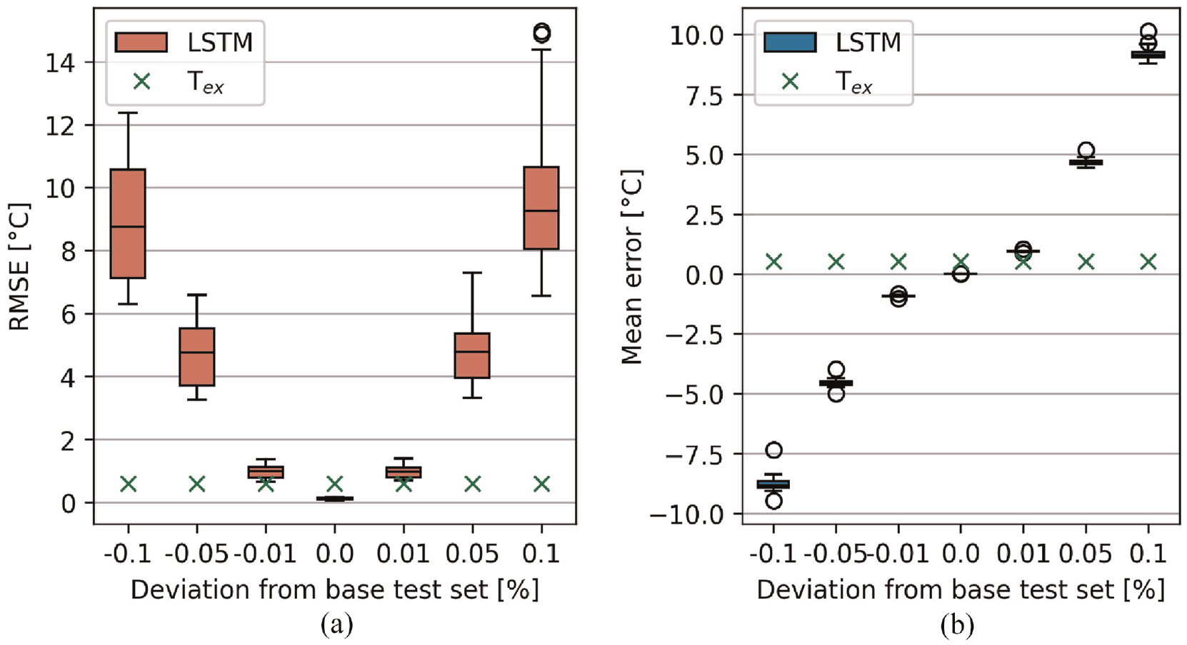
Performance metric boxplots for each trained network on the velocity OODD test sets. The percentage deviation refers to the
This can be intuitively explained by considering the following scenario. Consider a block of thickness
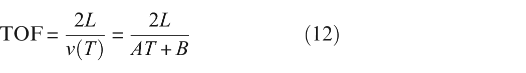
Suppose the TOF is measured at this given temperature, then the apparent temperature could be computed by rearranging Equation (12) using A+ and B+. The apparent temperature would underpredict the true temperature and hence this behaviour will be learnt by the network during training. The inverse of this effect was expected if
Figure 11 shows RMSE for the thickness OODD test sets. The metrics based on the external temperature are also shown as a reference. Similarly to the velocity OODD cases, the absolute magnitude of both the RMSE and mean error increase as the parameters (thickness) of the test sets diverge from the value used during training. However, it was expected that for the thickness OODD a positive deviation (OODD cases 4–6, Table 5) would cause the LSTM networks to over-predict the true temperature and therefore the error (according to Equation (10)) would be negative. This can again be explained by imagining a similar scenario as that described for the velocity OODD case except this block has true thickness
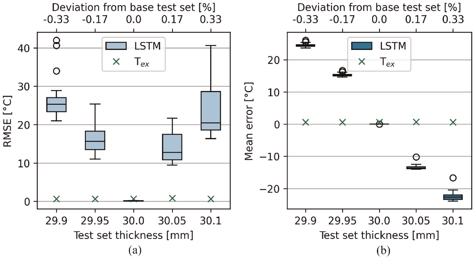
Performance metric boxplots for each trained network on the thickness OODD test sets. The base set (30.0, 0.0%) is included for reference. The box plots and crosses denote the metrics for the predictions by each of the LSTM networks and the external surface temperature, respectively. Prediction metrics for LSTM networks that were more than 1.5 × the interquartile range are shown by the circles. (a) RMSE, (b) mean error.
In both OODD scenarios, the RMSE and mean error in temperature prediction both grow with the increasing deviation of the training parameters. This error manifests as a constant offset which is shown by the mean error (Figures 10(b) and 11(b)). However, the RMSE box plots for both scenarios (Figures 10(a) and 11(a)) demonstrate that using an ensemble of many networks can help to diagnose this issue since the SD becomes larger as the deviation of parameters grows. This behaviour has previously been exploited for uncertainty quantification. 33 The influence of the size of the LSTM ensemble was not investigated, a smaller ensemble may be equally as informative whilst reducing computational expense. It should be noted that this issue of over/under prediction is also expected to be suffered by the ITM method and it is not possible to apply the ensemble method to ITM.
Experimental studies
The top panel of Figure 12 shows the mean predicted temperatures across the 25 LSTM networks with one SD above and below this value superimposed. The predictions by the ITM method as well as the embedded RTD measurements are also shown as references. The bottom panel of Figure 12 shows the errors based on Equations (10) and (11). To achieve the predictions shown in Figure 12,
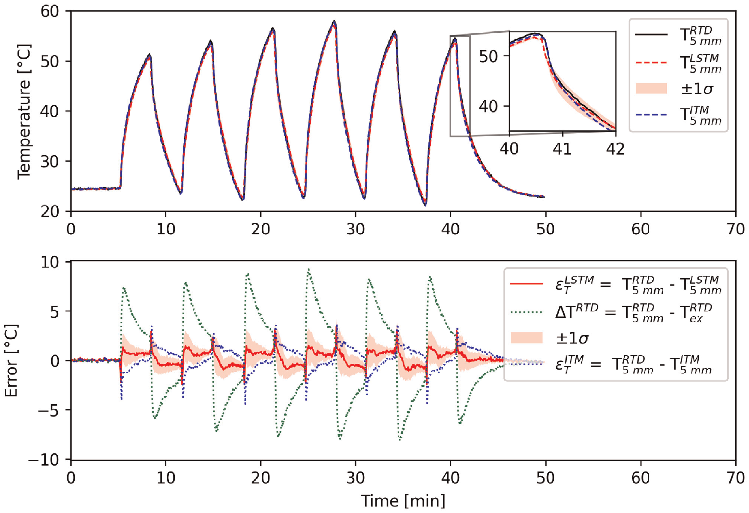
Experimental test set results. Top panel: RTD-measured temperature 5 mm from the water– metal interface
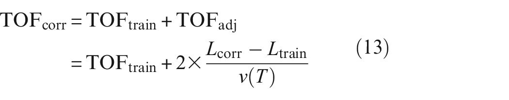
The corrected thickness,
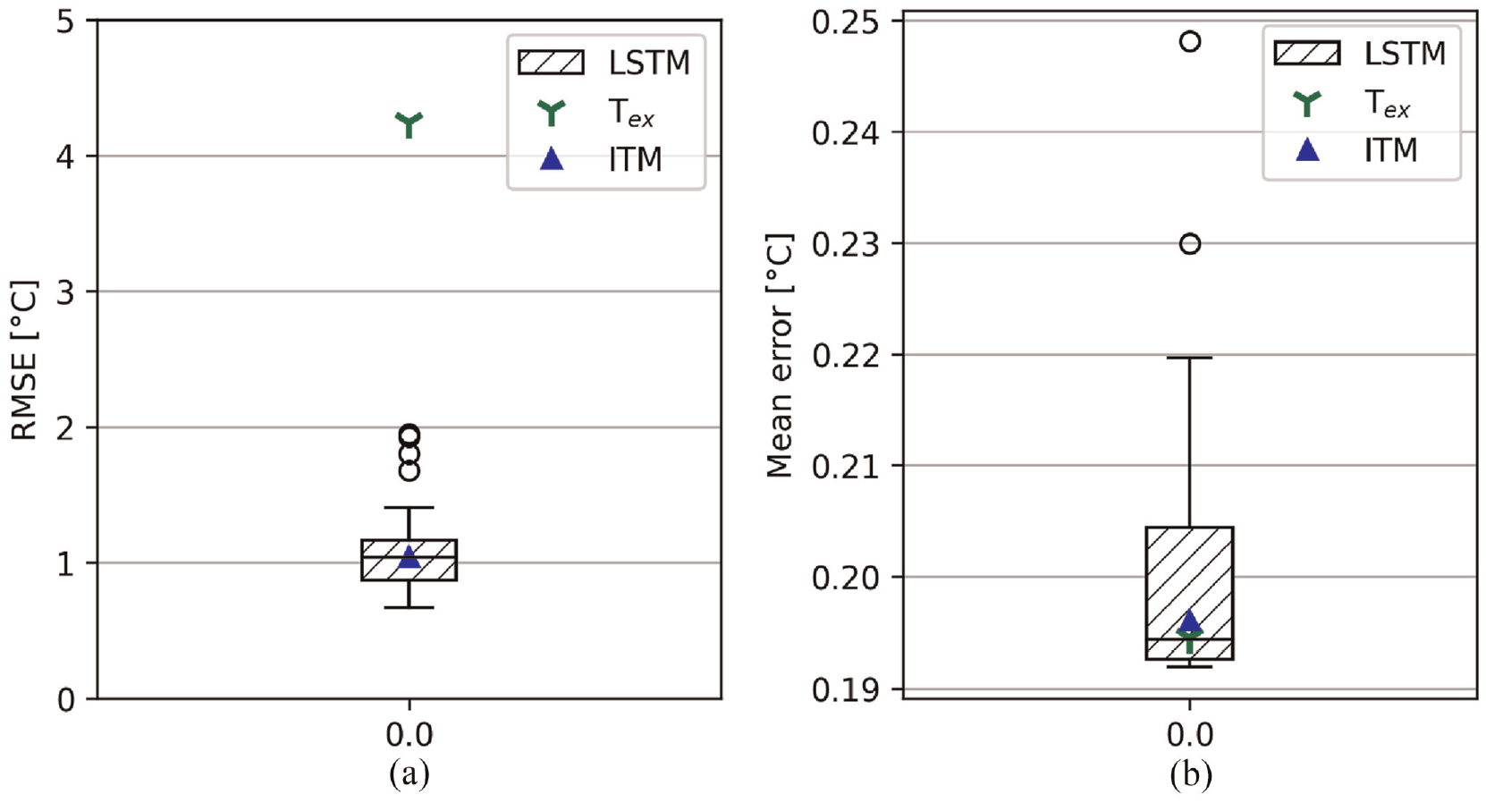
Performance metrics for the LSTM networks, ITM and external surface temperature predictions made on the experimental. The box plots, tri-stars and triangles denote the metrics for predictions by each of the LSTM networks, the external surface temperature and ITM method, respectively. Prediction metrics for LSTM networks that were more than 1.5× the interquartile range are shown by the circles. (a) RMSE, (b) Mean error.
The ITM implementation used a similar method to adjust the assumed thickness using the period in which the block temperature is uniform and then rearranging Equation (12) to obtain
Prediction time
The percentage ratio,
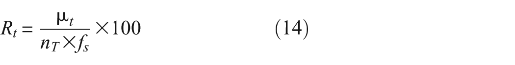
If
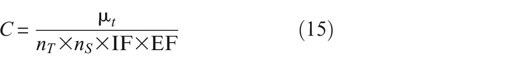
As in Equation (14),
Value of each correction factors used in Equation (15) to compute the adjusted mean computation times.
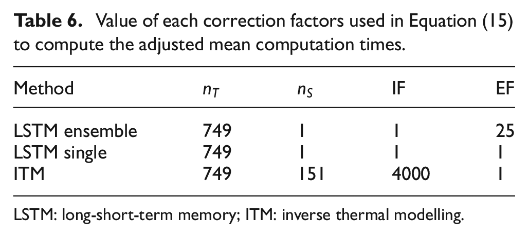
LSTM: long-short-term memory; ITM: inverse thermal modelling.
Table 7 shows both the raw
Raw mean computation time
LSTM: long-short-term memory; ITM: inverse thermal modelling.
For the prediction of temperature-gradient-induced stresses some form of spatial resolution is required. ITM satisfies this requirement as the full (151-node) spatial grid must be computed at each time step. In contrast, the presented LSTM networks only computed a single spatial point. Therefore, spatial resolution could be achieved using multiple LSTMs for different spatial locations (spatial ensemble). Since the raw computation time scaled for LSTM (approximately) linearly with ensemble size, it is expected that a spatial ensemble would follow a similar behaviour. This is not to say that a spatial LSTM ensemble would need 151 members (to match ITM) since this discretisation is expected to exceed the spatial resolution necessary for predicting the thermo-mechanical stresses that cause HCTF. Hence, the impact of increasing LSTM spatial outputs is not expected to increase LSTM prediction times prohibitively, that is,
Another factor to consider is that the experimental data sampling rate (0.25 Hz) would alias the maximum critical HCTF frequency at Civaux (1 Hz). Therefore, the measurement sampling frequency would have to be increased to at least 2 Hz
39
to properly capture 1 Hz fluctuations. At 2 Hz, the ITM method prediction time and
The adjusted computation times for each of the methods are expected to be sufficient for real-time monitoring considering the critical range of HCTF frequencies (0.1–1 Hz) for Civaux. Nevertheless, further investigation is required to determine whether these speeds are achievable on lightweight, field-deployable hardware. During the development of the LSTM and ITM codes, speed and efficiency were not prioritised. Therefore, the execution speed of both codes might be improved through careful programming of the respective methods. For the LSTM ensemble such techniques might include:
Reduction of the number of ensemble members
Conversion of the ensemble into a single compact ‘multi-headed’ network 45
Network simplification by pruning46,47 (also applicable to a single network)
Performing a hyperparameter search to remove network complexity, for example, number of neurons (also applicable to a single network)
It is important to highlight that the same 25-member LSTM ensemble was used throughout the simulation and experimental studies. The networks were all trained using pure simulation data yet were able to make predictions on experimental data which have similar accuracy as the ITM method (with a correction factor to address the difference between the assumed training data thickness and true experimental thickness). Furthermore, the LSTM networks were trained on simulated data sampled at 0.5 Hz. When predictions were made on the experimental data which were sampled at 0.25 Hz, no interpolation was applied meaning the LSTM networks were predicting on sparse data.
Conclusions
HCTF in NPP mixing zones is driven by large temperature gradients, that is, large differences between the interior and exterior wall temperatures in a pipe. It was previously shown that using the physics-based ITM method the inaccessible pipe wall temperature can be estimated to within 2°C by using the information from an external temperature measurement and the ultrasonic TOF. However, the ITM method was perceived to be relatively slow requiring 423 s to invert the full data set on a 12th Gen Intel core i7 processor CPU of a desktop PC. For field deployment less powerful processors would most likely be available and therefore this study investigated whether LSTM machine learning architecture would be less computationally intensive than the ITM method, whilst achieving comparable accuracy.
It was found that relative to a resistance temperature detector measurement, the 25-member LSTM ensemble achieved an ensemble median RMSE of 1.04°C and an ensemble median mean error of 0.194°C. This is almost identical to the performance of the ITM method which achieved a RMSE and mean error of 1.04°C and 0.196°C, respectively. These key metrics demonstrate that LSTM networks can perform as well as the ITM method if parameters such as the component thickness and velocity–temperature relationship coefficients used during training are in perfect agreement with the (unseen) test set. However, differences between the training and testing sets as small as
The aspects that affect computation time for a temperature prediction using both the LSTM and ITM methods were also discussed. While, for the implementations in this work, the LSTM looked considerably faster for performing temperature estimates for a full data set, the ITM method actually had a lower computation time per temperature estimate. However, for the stability of the ITM method it is required that it performs predictions at very small time steps, which therefore requires many interim computations if the sampling rate is relatively slow, that is, 0.25 Hz. This means that the ITM computation time will be unaffected by an increase in sampling rate, unless the increase exceeds the stable ITM time step. On the other hand, the LSTM method would need to perform more computations for an increased sampling rate, increasing computation time. A similar argument will apply in space; for the prediction of temperature-gradient-induced stresses some form of spatial resolution will be required. The ITM requires the use of a spatial grid of
Footnotes
Declaration of conflicting interests
The author(s) declared no potential conflicts of interest with respect to the research, authorship, and/or publication of this article.
Funding
The author(s) disclosed receipt of the following financial support for the research, authorship, and/or publication of this article: The authors would like to acknowledge funding from EPSRC for project funding as part of the FIND CDT (EP/S023275/1).