
Abstract
Accurate temperature measurement is a crucial aspect of structural health monitoring and prognosis. Conventional temperature measurement devices are either incapable of measuring subsurface temperatures in solids or need to be invasively installed. This study investigates the use of an ultrasonic technique for non-invasive measurement of subsurface temperatures in steel components; the temperature of a point on an inaccessible surface is inferred using a time-of-flight measurement from a transducer placed on an opposing accessible surface. Two different inversion approaches are presented, one named the assumed distribution method and the other named the inverse thermal modelling method. The robustness and accuracy of the two ultrasonic temperature inversion methods are quantitatively assessed via simulations and controlled experiments. It was found that both the assumed distribution and inverse thermal modelling methods demonstrate short thermal response times and are able to track the temperature evolution of inaccessible surfaces. A series of experimental studies show that in the presence of a 15°C difference between the accessible and inaccessible surfaces, the inaccessible surface temperature is typically measured to within better than 2°C with respect to a resistance temperature detector reference measurement. Additionally, the article compares the measurement performance achieved using a deployable electromagnetic acoustic transducer and a permanently installed piezo-electric PZT transducer. The time-of-flight measurements taken using the electromagnetic acoustic transducer system had higher random noise than the PZT system (standard deviations of 0.42 and 0.016 ns, respectively), subsequently leading to higher random noise in the temperature estimates.
Introduction
Motivation
Temperature is a crucial parameter in the analysis of many failure mechanisms such as thermal fatigue and creep. 1 Accurate temperature measurements are therefore important for the reliable assessment of the likely location and severity of the damage in a structure. Even the internal temperature of a simple pipe wall in high temperature pipework can be highly non-uniform (see illustration in Figure 1), especially during transient heating or cooling. Standard temperature measurement devices such as thermocouples or resistance temperature detectors (RTDs) can only measure the temperature of the surface onto which they are installed, normally the outside surface of the pipework. Temperature measurements at the accessible surface can lead to significant under or overestimation of the temperature at the inaccessible interior surface. There are techniques that measure subsurface temperatures, such as the use of thermowells.2–4 However, they need to be installed invasively with clear implications on cost and structural integrity.5,6 This article presents a method for estimating the temperature of an inaccessible surface using a time-of-flight (ToF) measurement from an opposing accessible surface.
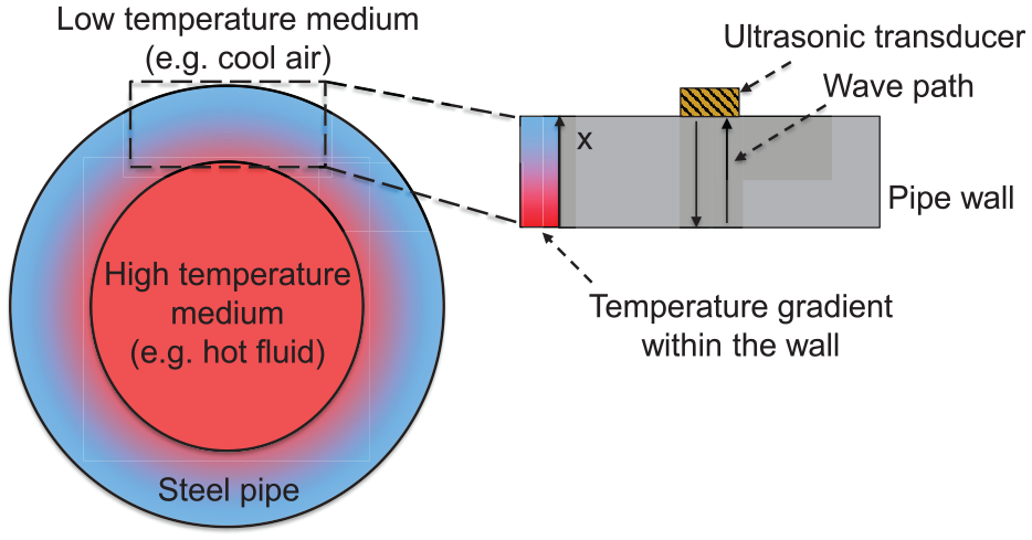
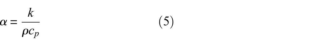
Schematic of a pipe cross section exhibiting a temperature gradient. The red colour denotes a state of higher temperature and the blue colour denotes a state of lower temperature.
Measurement principle
A simplified one-dimensional (1D) system, denoted by spatial coordinate
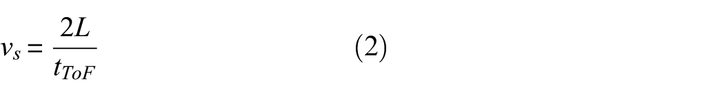
ToF is defined as the time taken for the ultrasonic waves to propagate along a designated wave path. If the wave path and velocity along the wave path are known, the time-of-flight,
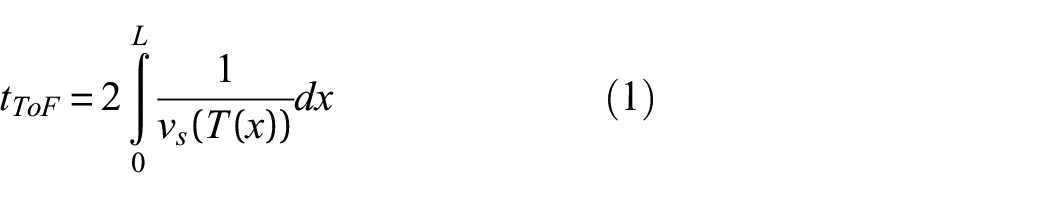
where
Figure 2 shows a typical signal collected by an in-house electromagnetic acoustic transducer (EMAT) 7 system employing coded excitation for highly repeatable ToF measurements. 8 The ToF is measured by determining the time between the peaks of the multiple echoes of the ultrasonic wave that reverberates within the specimen.
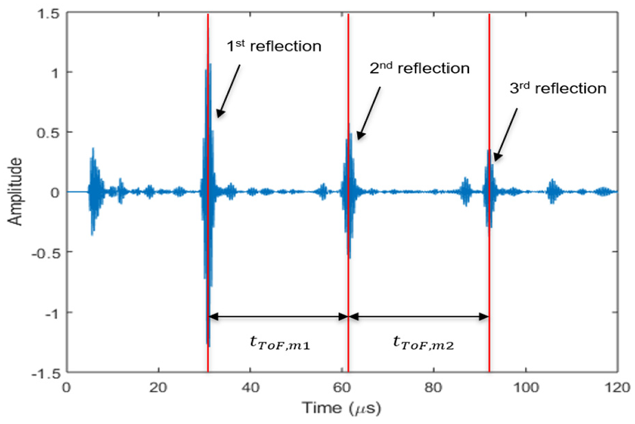
Typical signals measured using the in-house EMAT system on a 50 mm mild steel block
Figure 3(a) shows the temperature-dependent shear wave ToF in a 50-mm-thick mild steel (080A15/EN32B) specimen, where a linear function is fitted to describe the relation between ToF and temperature. The temperature–ToF relationship is obtained by quasi-statically cooling the specimen in a climate chamber, thus ensuring its internal temperature distribution is close to uniform. Detailed descriptions of the calibration experiment are presented in section ‘Experimental demonstration’.
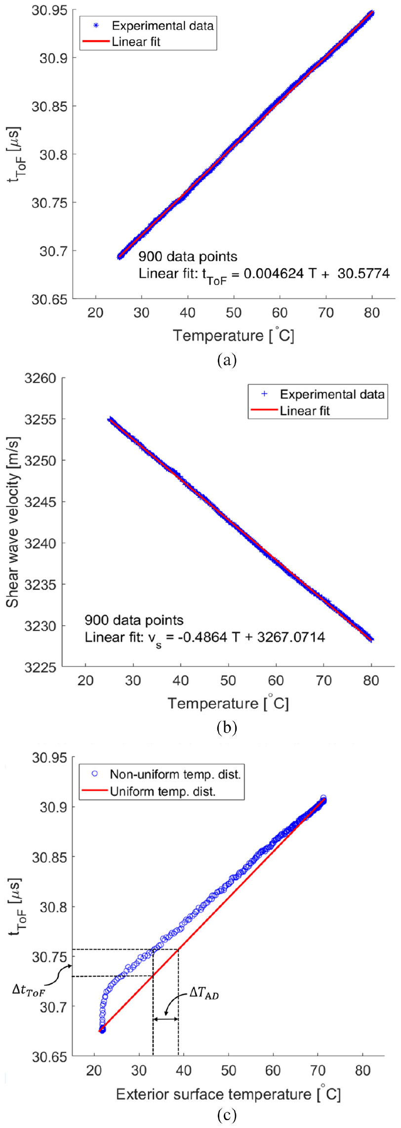
(a) Experimentally measured ToF variation against exterior surface temperature when a 50-mm-thick steel sample undergoes quasi-static cooling in a climate chamber. (b) Variation of inferred shear ultrasonic velocity against exterior surface temperature measurements during the quasi-static cooling. (c) ToF variation against exterior surface temperature measurements during transient heating of the specimen from the opposite surface.
On the contrary, the ultrasonic velocity can be inferred by dividing the length of wave path by the ToF. It is assumed here that the variation of ToF due to thermal expansion of the material is negligible compared to the variation caused by velocity change9,10
The variation of ultrasonic velocity arises from the temperature dependence of the density and elastic properties of the medium. 11 Although the exact underlying mechanisms are complicated, a linear relationship is also often used to describe the temperature dependence of ultrasonic wave velocity12–14

where
Figure 3(b) shows the variation of inferred shear ultrasonic velocity
While Figure 3(a) and (b) describes the temperature relation at quasi-static conditions, Figure 3(c) shows the variation of shear wave ToF with the exterior surface temperature (i.e. the temperature at the location where the transducer is installed) when the same specimen undergoes transient heating. During the transient changes, the relationship between ToF and accessible surface temperature deviates from the linear function shown in Figure 3(a). This is a result of a discrepancy between the accessible surface temperature the RTD is measuring and the temperature the ultrasound experiences as it propagates through the non-uniform through thickness temperature profile. It is this discrepancy between the expected and measured ToF that will be utilised to estimate the inaccessible surface temperature.
Previous work
The non-invasive nature of ultrasonic testing has gained attention in thermometry. Most ultrasound-based thermometry deduces temperature variation based on changes in ToF of the ultrasonic waves.15–19 Although there are other studies that deduce temperature from features such as phase changes 20 or changes in the resonance frequency and scattering characteristics, 21 the ToF-based method is the most straightforward approach and will be the focus of this article.
There are in general two types of ultrasonic thermometry: (1) bulk measurements where the temperature is assumed to be constant across the whole wave path 13 and (2) where the temperature varies along the wave paths and one tries to reconstruct the temperature field. While some research has investigated reconstructing temperature fields in gas or liquid media based on ultrasonic measurements,15,22 limited research has focused on the temperature reconstruction in solid media.23,24 In addition, although many reconstruction algorithms have been proposed to obtain the two-dimensional (2D) or three-dimensional (3D) temperature field within a system, most of the tomography methods utilise the through-transmission ultrasonic technique that requires multiple transducers and access to multiple location along the boundary of the system.
For single wave path measurements, Ihara et al.17,25 reported an inverse analysis method to obtain the internal temperature based on ultrasonic measurements. The ToF-based method coupled 1D finite difference calculation of the heat conduction problem with ultrasonic measurements. One favourable feature of the method is that the internal temperature profile can be obtained without having access to the inner (opposite) surface of the component. However, this direct inverse method is susceptible to numerical instability due to numerical errors and measurement noise. Shi et al. 18 and Wei et al.19,26,27 presented an inverse approach based on the sensitivity method. The authors of those studies argue that if the boundary conditions on both sides of the 1D system are known, the temperature distribution within the system can be simulated and ToF of ultrasonic waves travelling through it can be calculated. The calculated ToF should match the experimentally measured values if the applied boundary values are close to the actual ones. Hence, the unknown boundary value on the inaccessible end of the system can be searched in an iterative process by minimising the difference between calculated and experimentally measured ToF. The main limitation of this approach is that it requires continuous temperature and ultrasonic measurements and is relatively computationally expensive.
This article presents a measurement procedure together with two inversion techniques. The first is based on the method of Wei et al.;19,26,27 the method is generic but computationally expensive. The second is a novel approach that relies on an assumption of a linear through thickness temperature profile; the method is much simpler and can be completed without requiring near-continuous data. The performance of both inversion techniques is evaluated using simulated and experimental data. Additionally, the article compares the measurement performance that can be achieved using an EMAT with the performance that can be achieved using a permanently installed piezo-electric PZT transducer.
Structure of the article
The article is structured as follows: the section ‘Ultrasonic temperature measurement’ introduces the problem of heat transfer in a 1D system and a numerical method for simulating it. The methodology of the two ultrasonic temperature reconstruction algorithms is subsequently presented in the same section. The section ‘Simulated and experimental performance studies’ first establishes three key metrics used for assessing the performance of the ultrasonic measurement methods. The performance of the two inversion techniques are then tested on simulated data. Subsequently, the ultrasonic measurement methods are further tested on experiments, where different thermal conditions are imposed on the specimen. A comparison between the EMAT and PZT transducer measurement systems is carried out. Finally, the main findings of this study are summarised in the conclusions.
Ultrasonic temperature measurement
Heat transfer in an one-dimensional system
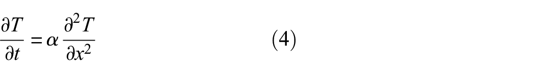
A 1D heat transfer model will be introduced in order to illustrate the anticipated non-linear temperature profiles that will be present in a system such as that shown in Figure 1. The understanding gained from an illustrative transient heating example will inform the inversion methods described in the subsequent sections and the model itself will be a constituent part of the inverse thermal modelling (ITM) inversion method. For the system that is illustrated in the inset of Figure 1, it can be shown that when the pipe is in thermal equilibrium with its surroundings, the temperature distribution within the pipe wall is linear and independent of time. The system is said to be in a steady state. In contrast, when the conditions within or outside the pipe are altered, the temperature distribution will also vary and settling time is required for the system to reach a new equilibrium state. The intermediate state is referred to as the transient state, during which the temperature distribution is time-dependent and generally non-linear. The heat diffusion equation (equation (4)) describes the variation of temperature in the transient state
where temperature
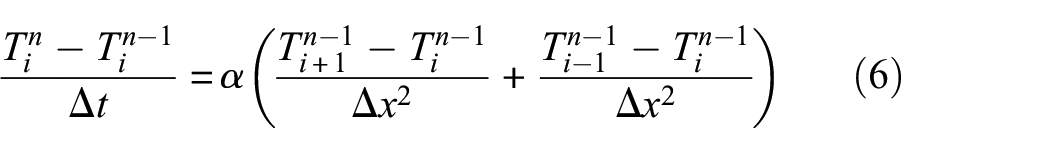
The heat diffusion equation can be solved either analytically or numerically; here, an explicit 1D finite difference scheme (see illustration in Figure 4) is applied to transform equation (4) into the discretised form (equation (6)). Equation (7) subsequently allows the temperature of a node at the current status
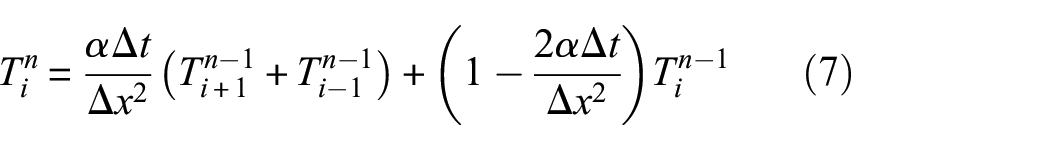
Convective boundary conditions and the principle of energy balance are implemented to define the boundary values

where

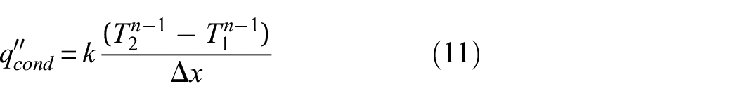
where
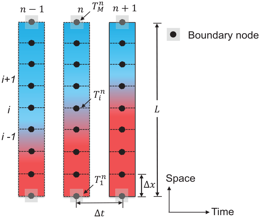
Discretised grids in time and space used in the 1D finite difference scheme. The subscript
Material property and boundary conditions applied in the simulation.
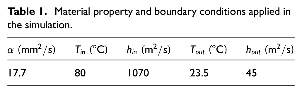
Figure 5 shows the temporal variation of temperature distribution. The simulations reveal that the temperature profile is expected to be highly non-linear during the initial phases of the transient state (subplot (a)). The implication of this is that inverting the inaccessible surface temperature becomes more challenging if the profile is non-linear. Second, the simulations reveal how the temperature gradient diminishes with time, (subplot (b)). Not only does the temperature profile become more linear but the temperature difference reduces. It is for this reason that this article will focus on the problem of transient temperature profiles as the most demanding application for remote surface temperature estimation.
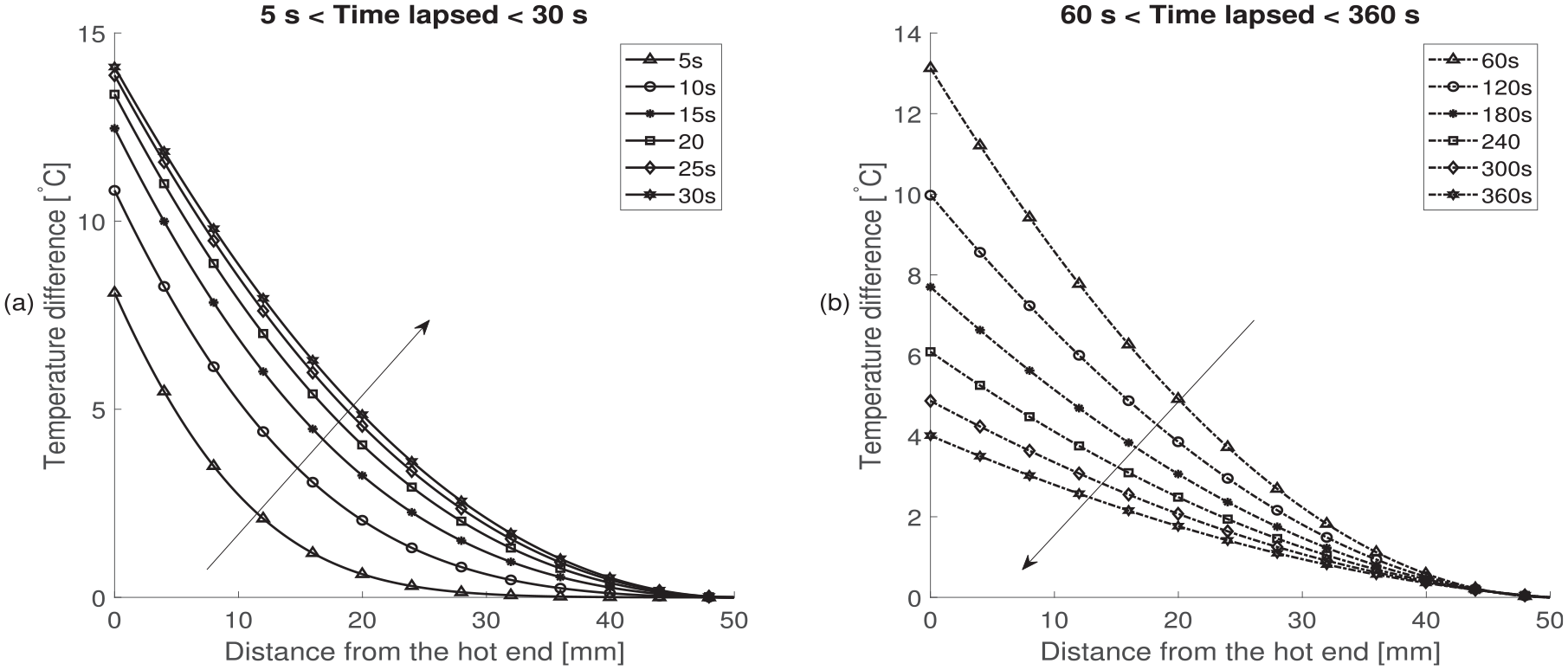
1D finite difference simulation of temperature gradient across a pipe wall during transient heating with the parameters outlined in Table 1. Variation of temperature difference across the pipe wall for (a)
Two inversion approaches have been investigated based on the understanding gained in the simulation. They will be presented in more detail in the following subsections.
Temperature estimation using the ITM inversion approach
The first inversion method is constructed following the approach outlined by Wei et al.19,27 and will be referred to as the ITM approach.
To calculate the temperature distribution at a certain time instance

where the superscript
The value of
where
If

else
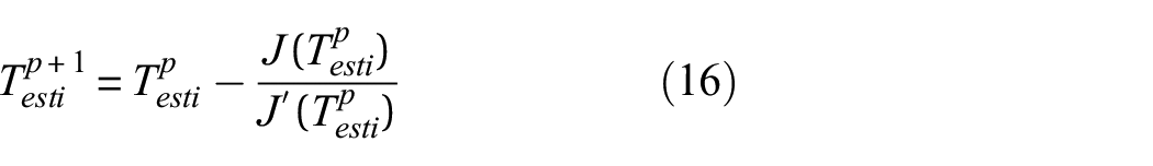
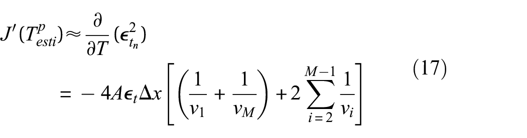
where
An important feature of the ITM inversion method is that the full through-thickness temperature profile is estimated and not just the inaccessible surface temperature. The profile estimated is an important input in thermal fatigue estimation. 28
The ITM inversion approach relies on a few essential requirements:
Knowledge of the uniform temperature–ToF relationship.
Knowledge of the initial temperature distribution within the component. In this study, the initial temperature distribution is assumed to be uniform.
Knowledge of the component thickness. The component thickness can be estimated from ToF measurements when the temperature profile is assumed to be uniform and the ultrasonic velocity at the temperature is known.
The thermal diffusivity of the material is assumed known and homogeneous. The material is assumed to be free from defects that may impede or distort the internal heat conduction process.
Availability of near-continuous (every few seconds) ultrasonic measurements and temperature measurements of the accessible surface.
The validity and influence of these assumptions will be explored in the experimental study and discussion.
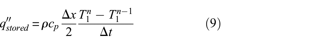
Temperature estimation using the assumed distribution inversion approach
The second of the inversion approaches is based on the assumption that the internal temperature profile is linear; clearly this assumption is not robust (see Figure 5), but the studies in this article will explore how satisfactory the estimates are using this highly simplified approach. This method will be referred to as the assumed distribution (AD) approach.
As shown in the introductory section, for a component with a uniform internal temperature distribution, the relationship between ToF and externally measured temperature can be approximated using a linear relation. However, if the internal temperature distribution is non-uniform, the observed ToF–temperature relationship becomes non-linear, as evident in Figure 3(c). The non-linearity is introduced due to a discrepancy between the temperature measured on the accessible surface and the temperature profile of the ultrasonic path. The difference between the measured ToF,
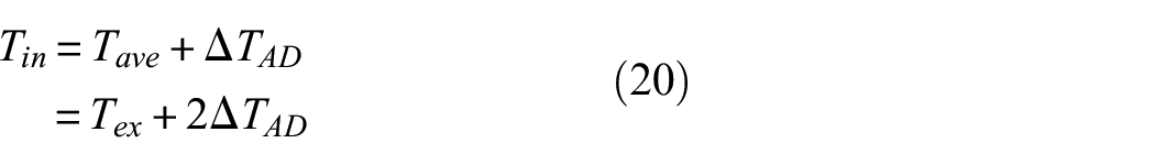
Assuming a linear temperature profile enables inference of the temperature of the inaccessible surface. Referring to Figure 3(c), the ToF discrepancy is given as

which allows estimation of the temperature difference
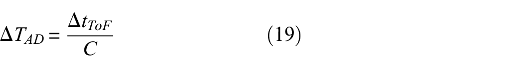
The value of
This AD inversion approach relies on the following key assumptions:
The temperature distribution across the pipe thickness is assumed to be linear. Clearly, this is not a robust assumption, as shown in Figure 5. The temperature gradient can be highly non-uniform in the transient state and assuming a linear relation will lead to underestimation of the inaccessible surface temperature. However, as the system transitions into the steady state, the temperature field will converge to a linear distribution and the associated estimation errors are expected to reduce along with it.
A key assumption underlying equation (19) is that the temperature implied by the ultrasonic measurement is equal to the average temperature of the linear temperature profile. This would be true if the ToF of ultrasonic waves propagating through a linear temperature profile with an average temperature of
The parameter
The pipe thickness is constant. It is assumed that there is negligible corrosion or erosion reducing the pipe thickness.
The material is assumed to be free from defects that may impede or distort the internal heat conduction process.
It is possible the performance of the AD method may be improved if more information regarding the system is known and an alternative or dynamic temperature profile can be assumed, but for the purpose of this study a linear profile will be assumed.
The main benefit of the AD method over the ITM method is that it does not rely on a near-continuous measurement; each new measurement can be interpreted in isolation and batch data processing is possible. Therefore, the AD method is simpler to implement and computationally inexpensive. A comparison between the computational costs of the two methods will be presented at the end of the next section. Unlike the ITM method, with the AD method only the inaccessible surface temperature will be estimated and not the full through-thickness temperature profile (as it is assumed to be linear).
Simulated and experimental performance studies
In this section, the performance of the ultrasonic-based thermography method will be demonstrated using both simulated ultrasonic signals and experiments. Both the ITM and AD inversion methods will be used and compared.
Assessment metrics
To assess the performance of the estimation methods, three main performance metrics will be used. All metrics are based on calculating the estimate residuals

where
Three key metrics, namely the average estimate residuals (ave
To provide a reference for the scale of the true temperature difference, a naive estimate is included throughout for comparison. The inaccessible surface temperature is assumed to equal the directly measurable accessible temperature; this would mimic the measurement accuracy in an industrial situation where a thermocouple or RTD is installed only on the accessible outside surface. This exterior surface measurement (ESM) provides a metric for contextualising the performance of the ultrasonic methods.
Simulated performance
The performance of the ITM and AD inversion approaches are first tested on simulated ToF data. This is calculated for a period of transient heating using the 1D thermal model. Subsequently, the two inversion approaches are used in order to estimate the inaccessible surface temperature.
The simulation consists of two phases: in Phase I
The convective boundary conditions applied in the validation simulation.
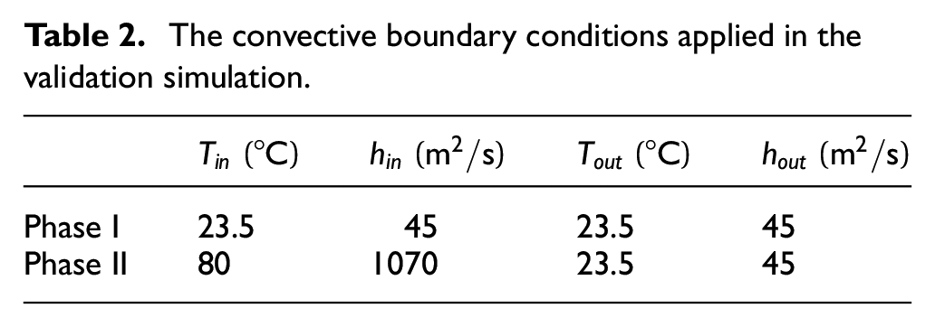
Figure 6 shows the simulated temporal evolution of ToF of ultrasonic waves travelling through the specimen in pulse-echo mode. Phase I and II in the simulation are colour coded in light blue and red, respectively. In addition, Gaussian noise with standard deviation of
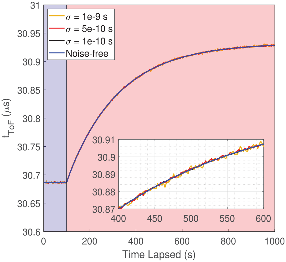
Simulated ToF of ultrasonic wave propagating in a 50 mm mild steel specimen in pulse-echo mode. The simulated ToF is also superimposed with Gaussian noise of
Figure 7 shows the simulated internal and external temperatures together with the estimates of the internal temperature inverted from the simulated ToF data of Figure 6. The ToF data with noise of
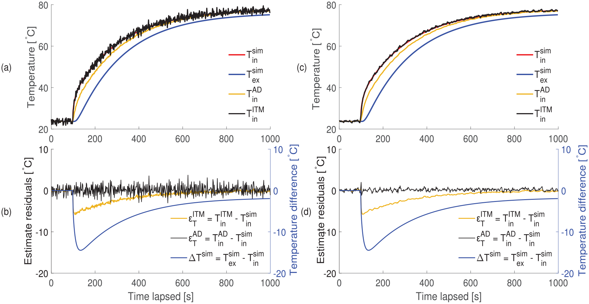
Comparison between the simulated interior surface temperature and the ultrasonic estimates. Gaussian noise of
Residuals of the temperature estimates under different levels of ToF measurement noise.
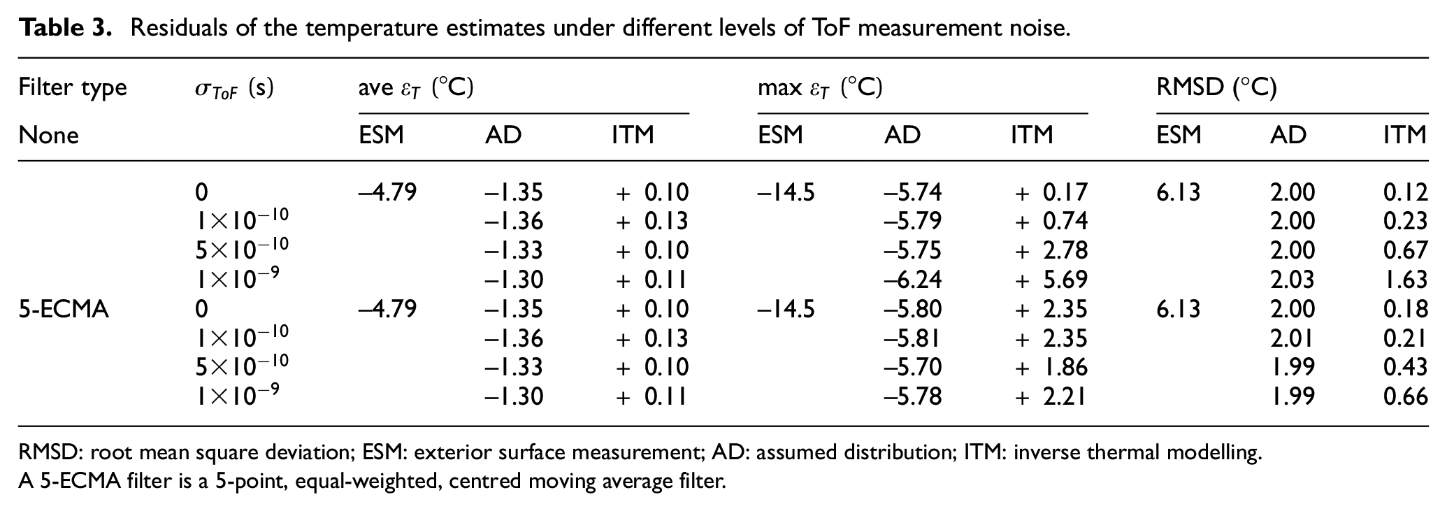
RMSD: root mean square deviation; ESM: exterior surface measurement; AD: assumed distribution; ITM: inverse thermal modelling.
A 5-ECMA filter is a 5-point, equal-weighted, centred moving average filter.
The estimates given by the ITM inversion follow the simulated values without significant bias. The lack of systematic error in this demonstration is not surprising as the same thermal model is used in both the forward model and inversion and all parameters are assumed to be known exactly; however, the iterative procedure is demonstrated to illustrate the feasibility of the procedure. The ITM estimates fluctuate around the simulated value due to the presence of the ToF noise. The authors believe that the ITM is particularly sensitive to ToF noise because rapid changes in ToF, that is, changes from one measurement relative to the next (as are introduced by the addition of Gaussian noise), are assumed to only occur in a small region of the material near the surface and they do not have time to diffuse through the material. Hence, the presence of ToF measurement noise will result in relatively large local temperature changes. This is different in the AD method where a temperature distribution is assumed and hence the change in ToF and temperature is averaged over the whole wave path. At this noise level, the RMSD of the ITM estimates is 0.67°C while the mean and maximum residuals are 0.10°C and 2.78°C, respectively. To reduce the estimate fluctuation caused by the measurement noise, a 5-point, equal-weighted, centred moving average (5-ECMA) filter is applied to both ultrasonic estimates and its effect is evident in subplot (c) and (d) of Figure 7. Based on the findings from the simulation, the 5-ECMA filter is applied to all of the subsequent ultrasonic estimates shown in this article.
A systematic error is evident in the estimates from the AD inversion method; the inaccessible internal temperature is consistently underestimated. The cause of the systematic error is a consequence of the underlying assumption of a linear temperature profile. The residuals are largest shortly after the onset of the transient heating flux when the temperature distribution is highly non-linear. The residuals reduce quickly as the system approaches steady state and the profile becomes more linear. Estimate fluctuations caused by the ToF noise are relatively insignificant compared to the estimate bias. At this noise level, the RMSD of the AD estimates is 2.00°C while the mean and maximum residuals are −1.33°C and −5.75°C, respectively.
Table 3 compares the effect of the superimposed ToF measurement noise on the two ultrasonic estimation methods; the table also shows the effect of data smoothing on the ITM method. It shows that the performance of the AD method is largely independent of the ToF noise, whereas the performance of the ITM method is adversely affected by the level of random uncertainty. The systematic error in the AD method is evident in the average residual metrics. The naive ESM metrics are provided for context.
Experimental demonstration
Temperature calibration
To obtain the ToF–temperature relation shown in Figure 3(a), a calibration experiment was performed in a dedicated climate chamber (VCL 4003, Vötsch Industrietechnik, Weiss Technik UK Ltd, The Technology Centre, Loughborough, UK). The specimen was heated up in the chamber by air to 90°C and was held at that temperature for 12 h to ensure it reached an equilibrium state (uniform temperature). The air in the chamber was then slowly cooled from 90°C to 20°C at a constant rate of 0.2°C per minute, and it was assumed that the temperature distribution within the sample was very close to uniform in the cooling phase. Ultrasonic and temperature measurements were taken every 20 s during the period.
Experiment arrangement
A number of experiments were carried out, but all had the same basic arrangement as shown in Figure 8. The specimen used in the experiment is a rectangular (100 mm × 50 mm) mild steel (080A15/EN32B) block of 50 mm thickness. The top and bottom surfaces of the specimen here correspond to the accessible exterior and inaccessible interior surfaces of a pipe structure. An RTD (RS PRO 2 wire PT1000 Sensor, class A, RS Components Ltd. Birchington Road, Corby, Northants, UK) was attached to both the top and bottom surfaces of the specimen and was covered by a layer of protective epoxy resin. Another RTD probe (RS PRO 2 wire PT1000 Sensor, class B, RS Components Ltd.) was placed into a water bath to monitor the water temperature. A magnetic stirrer was placed in the water bath; the stirrer speed can be adjusted between approximately 100 and 800 r/min. Temperature measurements were sampled by a data logger (PT-104 Platinum Resistance Data Logger, Pico Technology, St Neots, Cambridgeshire, UK). The sampling interval of the ultrasonic and temperature acquisition systems was set to 2 s. A linear interpolation method is used to up-sample the experimental measurements to ensure the numerical stability of the 1D explicit finite difference scheme used in the ITM method (equation (7)).
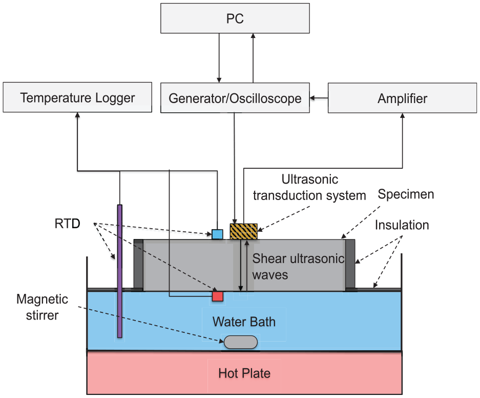
Schematic drawing of the experimental setup.
Table 4 summarises the test conditions of the five experiments documented in this study. Experiments 1–3 place a test piece into a water bath of 50°C, 65°C and 80°C, respectively, and a stirrer speed of 100 r/min. Experiment 4 uses a water temperature of 80°C and a higher stirrer speed of 800 r/min to produce a higher heat transfer rate. Experiment 5 differs from the rest as it utilises a PZT transducer instead of an EMAT.
Summary of the performance metrics for the ultrasonic temperature estimates.
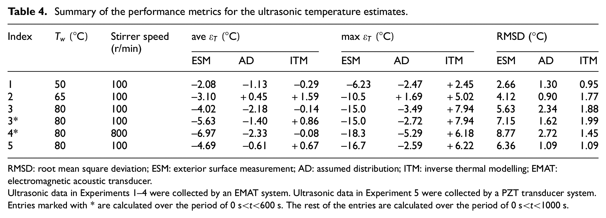
RMSD: root mean square deviation; ESM: exterior surface measurement; AD: assumed distribution; ITM: inverse thermal modelling; EMAT: electromagnetic acoustic transducer.
Ultrasonic data in Experiments 1–4 were collected by an EMAT system. Ultrasonic data in Experiment 5 were collected by a PZT transducer system.
Entries marked with * are calculated over the period of
Results and discussion
The first four experiments investigate the performance of the ultrasonic thermometry method on components with increasing heat transfer rates and therefore greater temperature gradients. Experiments 1–3 place the test component into water with increasing water temperature of 50°C, 65°C and 80°C, while Experiment 4 utilises a greater stirrer speed of 800 r/min compared to 100 r/min. The results are given in Figures 9 to 12 and the performance metrics are summarised in Table 4.
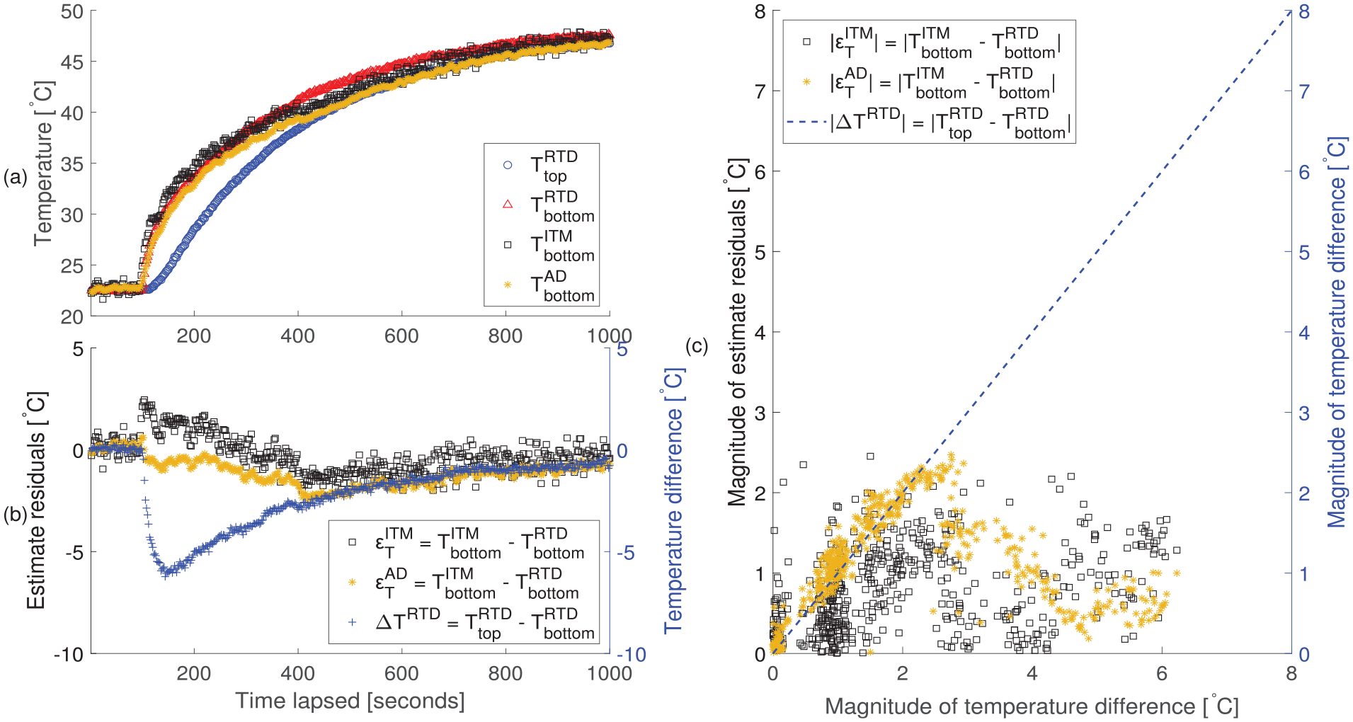
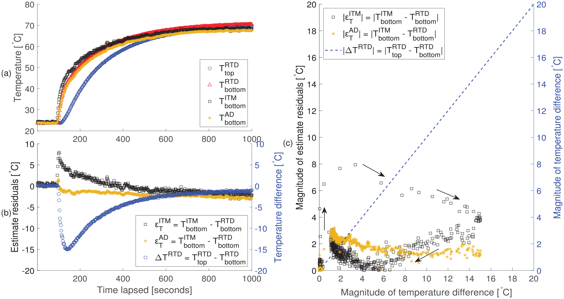
Results of Experiment 1 – experimental conditions: EMAT transduction system, water bath of
Results of Experiment 2 – experimental conditions: EMAT transduction system, water bath of
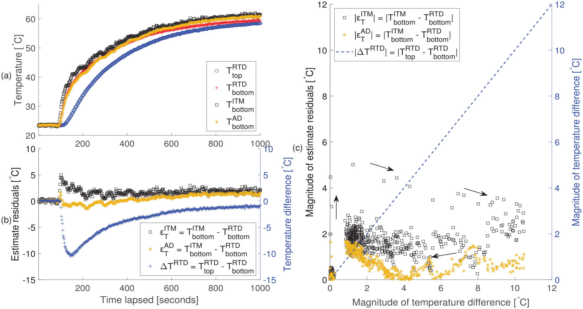
Results of Experiment 3 – experimental conditions: EMAT transduction system, water bath of
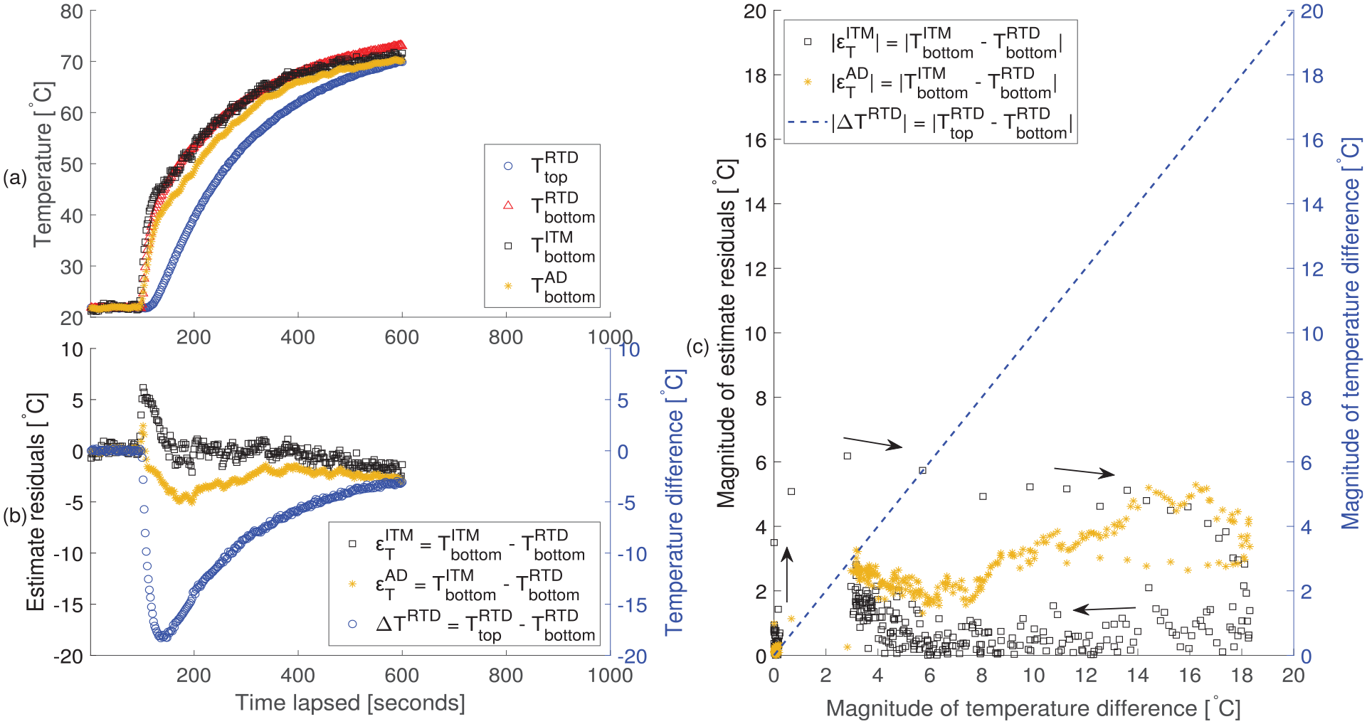
Results of Experiment 4 – experimental conditions: EMAT transduction system, 50 mm specimen,
For each experiment, the results are visualised with three subplots. Subplot (a) shows the temporal evolution of the RTD measured top and bottom surface temperatures together with the estimates of the bottom surface temperature from the ITM and AD inversions of the ultrasonic measurement. For improved clarity, subplot (b) shows the temporal evolution of the RTD measured temperature difference together with the temperature estimates of the inaccessible surface relative to the RTD measured value (i.e. the estimate residual). Subplot (c) is a scatter graph of estimate residuals against magnitude of the temperature difference; this is included to show that the estimate residual is not dependent on temperature. Subplot (c) also illustrates whether the temperature estimates are superior to the naive ESM estimator, indicated by data being to the bottom right of the blue line.
From Figures 9 to 12 and Table 4, the results of each experiment show broadly similar trends. In each experiment, the AD inversion method has a much smaller maximum residual than the ITM. Table 4 shows that the maximum residual for the AD method is typically around 2°C–3°C, but in Experiment 4 it reaches 5.29°C. The larger error in Experiment 4 could be a consequence of the higher heat transfer leading to a more non-linear through thickness temperature profile. The maximum residual for the ITM is typically of the order of 5°C–8°C. Table 4 shows that in general the ITM method has lower average residuals than the AD method. The reason is evident in subplot (b) of Figures 9 to 12; despite the smaller maximum residual, the AD method has a slightly larger residual later on which aggregates into a larger average residual.
Subplot (b) and (c) show that for each experiment, almost without exception, the ultrasonic measurements are superior to the naive ESM estimator. The understanding of the inversion process informs us that it is a rapidly changing non-linear temperature profile that coincides with high temporal temperature variation rate, dT/dt, that is more likely to be the cause of errors, this is also evident in Subplot (b).
The second part of the experimental study explores the use of a permanently installed PZT transducer for ultrasonic data acquisition. The permanently installed PZT transducer shows better ToF measurement repeatability at steady state and its output response is known to be more consistent over the temperature range. In this case, the ToF measurement repeatability (standard deviation) of the PZT and EMAT systems at 20°C are
Figure 13 shows the ultrasonic estimates of the PZT system in Experiment 5, where the specimen was placed in the water bath of 80°C. Compared to the EMAT estimates in Experiment 3, the PZT transducer estimates show much less random error. In addition, despite the presence of a larger temperature difference, both inversion approaches show improved accuracy as reflected by the decrease in the three key metrics. No significant under- or over-estimation is observed at the quasi-steady state towards the end of the experiment.
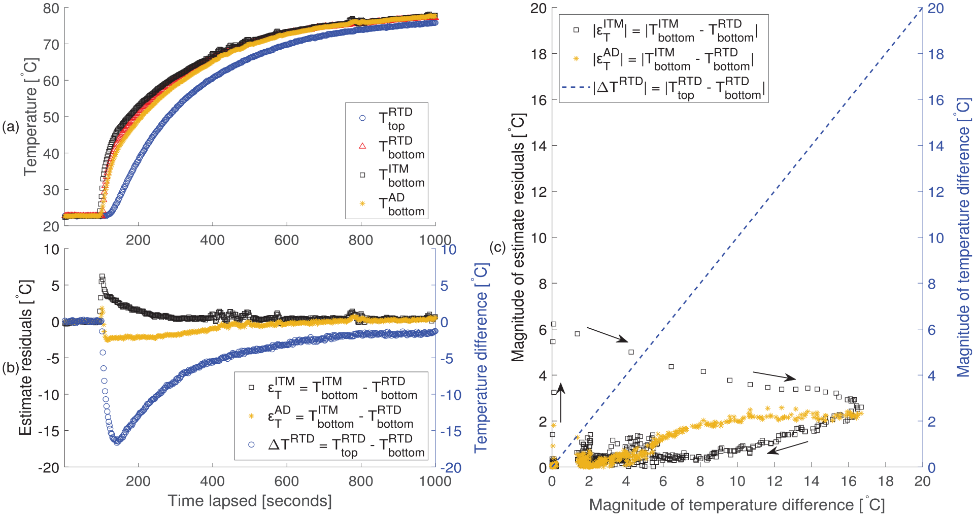
Results of Experiment 5 – experimental conditions: PZT transduction system, 50 mm specimen,
A few notes are made on the experimental results and discussed:
1. The estimate residuals of the ITM method appear to be worse than in the simulation, whereas the estimate residuals of the AD method appear to be better than that in the simulation. The authors believe that this is because in the simulation the actual temperature is known, whereas in the experiment the results are only compared to a reference measurement. The reference measurements (RTD) add an additional time lag to the recorded data. The ultrasonic measurement techniques, on the other hand, do not suffer from this time lag because they probe the material directly and do not rely on heat being transferred into the measurement device. The lag in the reference RTD measurements would tend to ‘exaggerate’ the errors of the ITM method and ‘suppress’ the errors of the AD method. This can be tested in simulation.
Figure 14 illustrates the effect of the time lag using simulated data. The addition of the time lag causes the residuals of the ITM estimate to spike at the onset of transient heating and suppresses the residuals of the AD estimates. There is good resemblance between subplot (b) and (d) of Figure 14 and Figure 13– the experimental results in Experiment 5.
2. The systematic error approaching steady state may be due to the assumed linear relation of ultrasonic ToF and velocity with temperature. The ultrasonic transduction system itself contributes to the measured temperature–ToF and temperature–velocity relations; subtle changes introduced by the transduction system could distort the measured relations. An EMAT involves the interaction of electric and magnetic fields, which are known to be temperature sensitive29,30 and may therefore produce such a systematic error. Experiments 3 and 4 have larger systematic errors which may be explained by the higher steady-state temperature (and therefore EMAT temperature). The PZT results have minimal systematic error which may be due to a more reliable relation of ultrasonic ToF and velocity with temperature.
3. With regard to the computational cost of the two methods: on a laboratory PC with 32 GB of memory and a 4.20 GHz processor (Intel Core(TM) i7-7700K CPU), the computational time of the ITM method to process 500 experimental data points was 20.79 s. In contrast, the computational time of the AD method on the same machine for the same data set was 0.001 s. Hence, the difference in the computational cost of the two methods is significant. On a field-based processor with limited computational capacity and power consumption restrictions, the choice of the AD method over the ITM method may be justified.
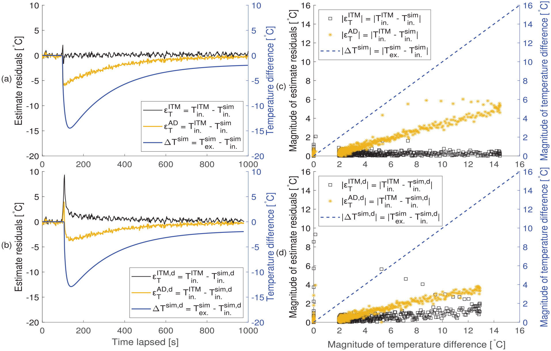
Comparison of simulated surface temperature and ultrasonic estimate residuals, with and without time delayed. No time delayed is applied in subplots (a) and (c); a time delay of 8 s is applied to the simulated interior surface temperature in subplots (b) and (d). Subplots (a) and (b): temporal evolution of ultrasonic estimate residuals and simulated temperature differences. Subplots (c) and (d): magnitude of the ultrasonic estimates residuals against the temperature differences.
Conclusion
This study investigates the use of ultrasonic techniques for taking non-invasive measurements of subsurface temperature in solids. Two different inversion approaches, the AD and the ITM method, are reviewed and their capabilities have been assessed through five controlled experiments. Key findings of the study are summarised in this section.
Both the AD and ITM methods show short thermal response times and are able to track temperature variation on an inaccessible surface. Under all the different tested thermal conditions, the ultrasonic estimates offer significant improvements when compared to the naive estimate based on an RTD measurement of the accessible specimen surface.
The AD method is very easy to implement and is computationally inexpensive. Each measurement is independent of the others so that the method does not require continuous measurements or information on temporal history of temperature. It is shown to underestimate the variation in temperature during rapid changes in thermal conditions. The performance of the AD method may be further improved if more information regarding the system is known and an alternative temperature profile is assumed.
The ITM method is in principle a more robust method as it does not rely on an assumption of a linear temperature profile. While the ITM method had greater absolute residuals than the AD method, in general it had lower average residuals due to the slightly superior steady-state performance. A possible reason for the larger maximum errors may be that the RTD measurements themselves lag behind the real temperature in the specimen and the ultrasonic measurements having a faster reaction time. The main limitations of the ITM methods are related to its complexity, as it requires near-continuous measurements and temporal history of the temperature change. The associated computational cost of the ITM method is also higher than that of the AD method.
The ultrasonic techniques have demonstrated potential to be part of a real-time monitoring and control system. The choice of permanently installed PZT transducer or deployable EMAT as the transduction system depends on the requirement of accuracy and nature of the task. It is believed that the performance of both estimation methods can be improved with enhanced experiment and hardware design and modified data-processing methods. Nonetheless, this series of experimental studies has shown that in the presence of a 15°C difference between the accessible and inaccessible surfaces, the inaccessible surface temperature can be measured to within 2°C of an RTD reference method by using the ultrasonic ToF information.
Footnotes
Declaration of conflicting interests
The author(s) declared no potential conflicts of interest with respect to the research, authorship and/or publication of this article.
Funding
The author(s) disclosed receipt of the following financial support for the research, authorship and/or publication of this article: The authors acknowledge financial support from the UK RCNDE that enabled this feasibility study.