
Abstract
Thermal integrity testing has been successfully used to assess the quality of cast-in-place piles for the past decade. It employs temperature data measured during concrete curing to identify defects along the piles’ length. However, the uptake of this technology has been rather limited in the piling industry. The main concerns are that the method is not standardised and its reliability is not well understood. In order to address these, there are a number of fundamental questions that need to be explored in more detail, including (a) the optimum time to conduct the assessment, (b) the defect thermal impact, (c) the zone of influence on temperature sensors, (d) the minimum detectable size of a defect and (e) the associated optimum sensor location required. In this paper, experimental and numerical studies were conducted to examine these questions. Fibre optic sensors were employed on model concrete piles in laboratory tests to provide fully distributed temperature data throughout the curing process. The test results showed that the optimum time to assess the defects is approximately at 60% of the time to reach peak temperature and the minimal detectable defect size, using the currently available optical fibre sensor technology, is 4% of the cross-sectional area. In addition, the thermal influence of different defect sizes is presented. Following this, it is shown in the paper that the minimum numbers of sensor cables required to identify defects with cross-sectional areas of 4%, 5% and 8% are eight, six and four cables, respectively. The optimum layout of these sensor cables within a pile cross-section has also been discussed. When specifying pile instrumentation for integrity assessment, the findings of this paper enable practising engineers to make informed judgements in relation to the size of defects they would like to detect (and hence the associated risk this entails) together with the corresponding instrumentation layout required.
Keywords
Introduction
Deep piles are commonly used for large superstructures, such as skyscrapers and long-span bridges, due to their ability to support heavier loads and overcome poor soil conditions by stretching deep into much stronger soil/rock. In addition to the standard design procedures, practising engineers also need to assess the as-built integrity of the piles to ensure their satisfactory performance as set by the design requirements.
Cast-in-situ concrete piles are prone to structural imperfections. A study of 2986 drilled shaft piles in California between 1996 and 2000 found that more than 20% of drilled shafts contained serious defects that could affect the piles’ structural integrity and thus could jeopardise the geotechnical load capacity. 1 A later survey 2 provided a 25-year pile testing record of more than 5000 cast-in-place piles in Germany and showed that approximately 15% of all the piles had significant defects.
The aforementioned problems may arise at different stages of the pile construction, from casing, drilling, concreting to slurry management. Typical piling defects can be classified based on their properties and mainly include soil intrusion, bulb, neck, crack, waist and expansion, as demonstrated in Figure 1.
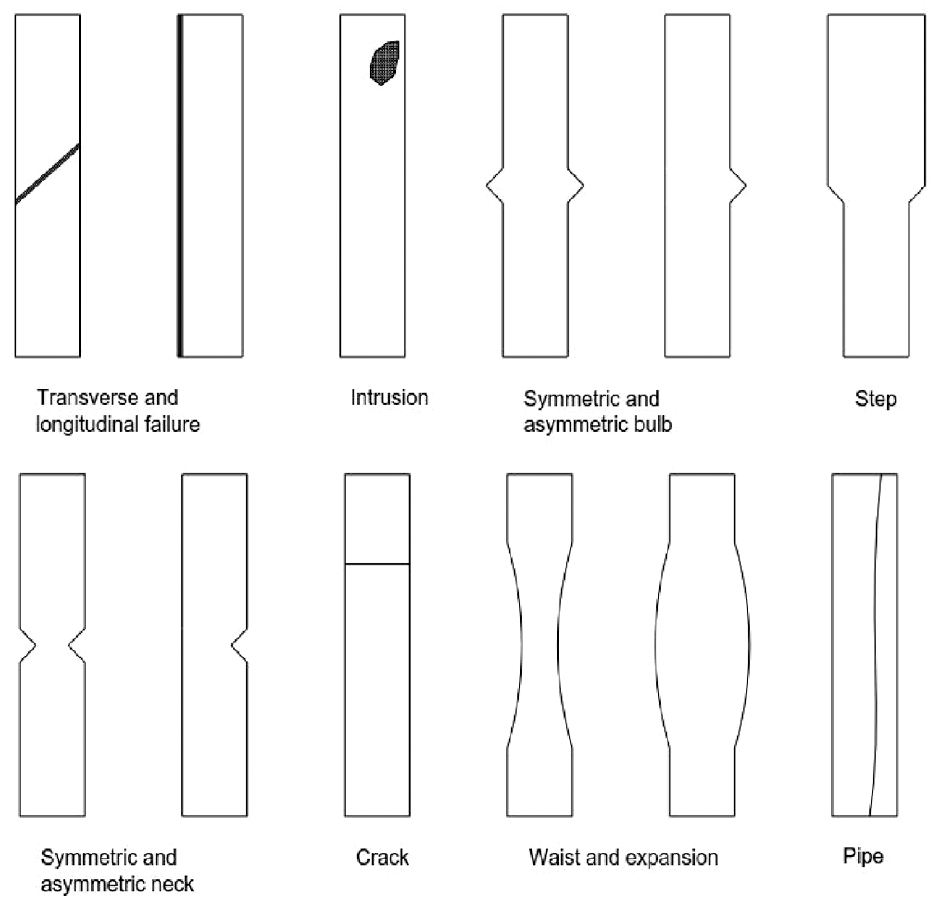
Typical defects for cast-in-situ concrete piles. 3
These pile defects have the potential to compromise structural stability or result in significant durability concerns. Early repair or reconstruction is crucial in preventing further damage and ensuring the pile’s integrity. As the cast-in-place piles are buried into the ground, they cannot be visually inspected in the same way as the structures above the ground. Therefore, the assessment of piles usually needs inference and engineering judgement which needs to be exercised on standard direct and indirect testing of the individual piles.
Traditional pile integrity tests, including sonic echo testing, crosshole sonic logging (CSL) and gamma-gamma logging (GGL), are all commonly used to help practitioners assess the condition of the piles. A wide range of potential anomalies could exist in the piles including voids, soil intrusions, cross-section variations, etc…; while each one of these traditional integrity testing methods has advantages and disadvantages, some are either less effective on certain types of defects than others or completely incapable of detecting certain types of defects.4,5 For example, CSL, the most widely used integrity method in practice, is able to detect defects inside the reinforcement cage well, but it cannot detect concrete cover problems at all. Moreover, during installation, connecting CSL access tubes pose a potential safety risk to site personnel as they negotiate the connections through the reinforcement cage. In recent years, electromagnetic waves (EMW) have been developed for pile integrity testing to overcome the disadvantages of CSL.6,7 Electrical wires are installed alongside the main rebars of the reinforcement cage to configure transmission lines so that the defects around the reinforcement cage are evaluated. EMW is a promising integrity method that does not require access tubes and is less expensive. Nonetheless, field tests are needed to validate the EMW integrity test capability in practice.
A relatively new method, thermal integrity profiling (TIP), has been put into use to assess the integrity of cast-in-place piles in practice during the past decade. TIP relies on measuring the thermal profiles of concrete in the piles during the concrete curing process. Heat generation and dissipation of early-age concrete are determined by the concrete mix, the ground conditions and the geometry of the concrete structure. If defects exist inside the concrete body, they will result in local temperature variations when compared to the expected heat generated during curing. As such, the measured temperature data are used to infer the as-built shaft shape, the centrality of the reinforcing cage and the possible existence of anomalies.
TIP testing has been successfully implemented in many construction sites both in the United States and the United Kingdom.4,5 The test results showed that TIP outperforms other integrity testing methods in a number of aspects:
The testing procedure is simpler and safer to execute on-site. The deployment of thermal wires and the collection of data require less manual input and time. Without the access tubes, used for CSL and GGL, the test does not pose additional safety risks for operators during the casting process. In addition, site engineers can conveniently observe the temperature profiles immediately following casting and hence, any severe defects could be identified in a timely manner.
TIP requires lower engineering and time costs. The average consumable and labour cost for each shaft is 43% less than CSL from a study of seven tests in the United States. 8 In addition, as the test is performed within the first day after concrete placement, this shortens the delay between pile construction and acceptance and allows an accelerated construction schedule. 9
TIP can evaluate the entire cross-section of the pile at any given depth; with particular emphasis on the outmost layer of concrete (as the temperature sensors are normally located close to the edge). By contrast, CSL evaluates concrete inside the reinforcement cage directly between the access tubes; GGL can only assess the concrete density around tubes within around 100 mm radius. 10
Although the thermal integrity test outperforms the traditional integrity testing methods in serviceability, cost and detectability and can provide more information about as-built shafts, however, the uptake of this technology is rather limited in the piling industry and far less common in comparison with CSL or GGL. First, the assessment steps to be followed are not explicitly documented in either the current standard 11 or the thermal integrity testing-related literature.10,12,13 Second, fundamental questions about optimum sensor configuration within a cross-section, sensor resolution, detection range, anomaly size and the optimum time to conduct an assessment remain a significant gap in the knowledge base. Moreover, short of digging the pile out, the data interpretation results in practice are difficult to validate; hence, this could explain the reluctance of the industry in adopting TIP widely.
The work presented in this paper attempts to address the fundamental questions mentioned above. Laboratory thermal integrity testing of two model piles cast in dry sand was conducted in which distributed fibre optic sensors were used to measure the thermal profiles along the model piles during the hydration process. The Luna ODiSI 6100 Analyser, which adopted optical frequency domain reflectometry (OFDR) technology, was used to collect temperature data from the optical fibre sensors. The two model piles had the same geometry and they were subjected to a consistent testing procedure. One of them had engineered inclusions installed before concrete casting while the other was inclusions-free. Both piles were excavated out from the dry sand 7 days after the casting for visual inspection. Temperature data was continuously collected, along the entire depth of the model piles, throughout the tests.
The conventional thermal integrity test uses embedded thermal wires, which consist of a string of discrete temperature sensors spaced typically at 300 mm. This could result in ‘blind spots’ in between the sensors depending on the size and location of the anomaly as well as the resolution of the sensor and the detection range. Without careful consideration of these factors, it is very difficult to have a reliable result that could be used by practitioners. The fibre optic temperature sensors used in this lab study provide a much higher spatial density of data of 400 sensing points per meter. This eliminates the issue of the blind spot in the lab and provides the opportunity to examine some fundamental questions detailed below.
The next section describes the measuring principle of the fibre optic sensing technique used in this paper. The laboratory testing procedure and the data analyses are presented next. The data analyses section examined the following fundamental aspects of thermal integrity testing:
The optimum time for the test data analysis (When is the optimum time to look for defects?)
The defect thermal impact (How do different size and shape defects affect the temperature distribution?)
The range of thermal influence for defects of different sizes (How far/close do the defects need to be before they are detected by the current instrumentation?)
The minimum detectable defect size (For a given pile geometry, what is the smallest defect that could be detected using the current instrumentation?)
The optimum layout of optical fibres and the minimum number of fibres to identify defects (What is the optimum way to arrange the instrumentation in a cross-section to enable the detection of a specified defect size?)
Discussion of the testing results and recommendations for practitioners are also included.
Fibre optic sensing measuring principle
In this study, temperature data was collected from fibre optic sensors (FOSs) using the Luna ODiSI 6100 Analyser (see Figure 1(a)). The sensing principle used in these types of analysers is OFDR, which is based on the Rayleigh scattering of light and could provide accurate distributed measurements at very high spatial resolution (millimetre-scale). 14 Rayleigh scattering exhibits no frequency shift compared to the laser input. OFDR uses a tunable or swept laser to measure the phase and amplitude of the Rayleigh backscatter signal in a fibre optic cable. A Fourier transformation is applied to obtain the signal in the optical frequency domain as a function of length. When the fibre is subjected to a strain and/or temperature change, a cross-correlation is performed for each gauge length to determine the spectral shift between the reference and perturbed scans. The spectral frequency shift, also known as Rayleigh backscattering spectra shift, recorded by the analyser is linearly related to the change in strain and/or temperature (for moderate temperature and strain ranges).14,15 This type of analyser can achieve a measurement resolution of 1 με and 0.1°C. The maximum length that can be monitored is between 10 and 100 m, depending on the special resolution and sampling rate (there is a trade-off among these three settings). When the measurement length is 10 m and the sampling rate is 20 Hz, a spatial resolution of 0.65 mm could be achieved. These features make the analyser ideally suited for laboratory use and small-scale physical modelling due to their relatively short distance and fine resolution.
The use of OFDR for structural health and geotechnical monitoring is described by Schenato et al. 16 Practical implementations using the commercially available OFDR devices include monitoring of reinforced concrete beams and bridges,17–19 railways, 20 steel trusses, 21 piles22–25 and soil anchors. 26 The analysers can be set up with commercially available fibre optic sensing cables; there is a multitude of optical fibre cable types commercially available with varying degrees of sophistication in their design. While robust cables are required for field applications, heavy reinforcement is likely to affect the transfer of strain to the optical fibre. Given that the research study was conducted in controlled lab conditions, there was no need to use heavily reinforced optical fibre cables.
When recording with an OFDR analyser, the change in spectral shift,
The frequency changes due to the coupled response to both temperature and strain changes. It is therefore important when monitoring either strain or temperature to ensure that the change in the other component is minimised or measured independently to remove its effects afterwards.16,27,28
In this test, a standard gel-filled loose tube temperature cable, as shown in Figure 2, was used to eliminate the strain influence. The polyvinyl chloride (PVC) gel-filled loose tube contained four 250 µm single-mode fibres and was encased in a 6 mm diameter cable with an outer sheath protection made of plastic. The fibres laid inside the water-blocking gel are free from minor stress. The external strain from thermal/mechanical stress cannot be directly transferred to the fibre in this type of cable.
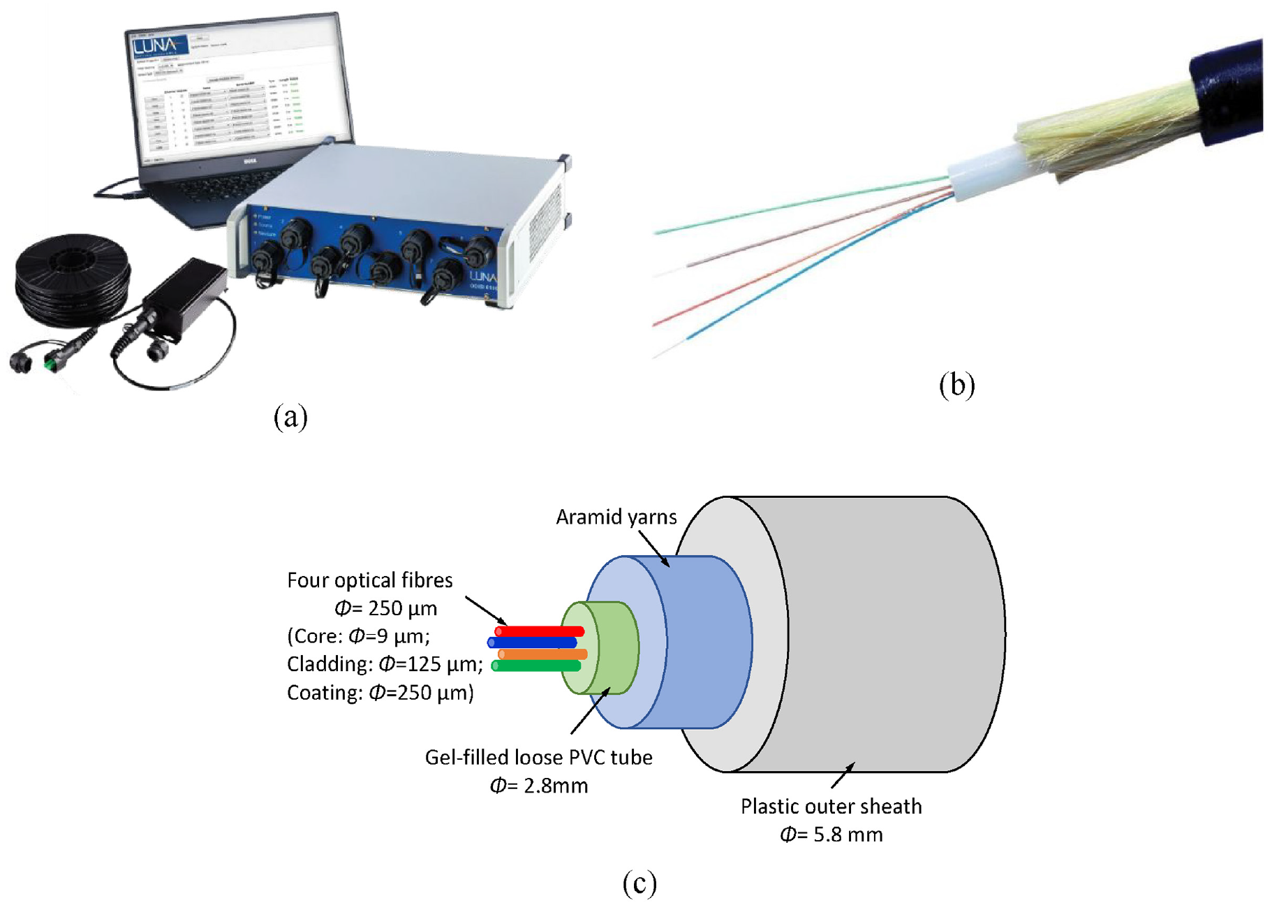
(a) ODiSI 6100 Luna OFDR analyser, (b) Gel-filled temperature cable, (c) Temperature cable configuration.
A schematic of the measurement system for the fibre optic sensing-based thermal integrity test is illustrated in Figure 3. The fibre optic temperature cables are vertically attached to the reinforcement cage using cable ties. For the convenience of data measurement, all longitudinal cables are looped or joined as a single wire. The cable is directed to a secured monitoring point and connected to the optical interrogator, where data measurement and collection are carried out. This image also displays an illustration of the temperature profile.
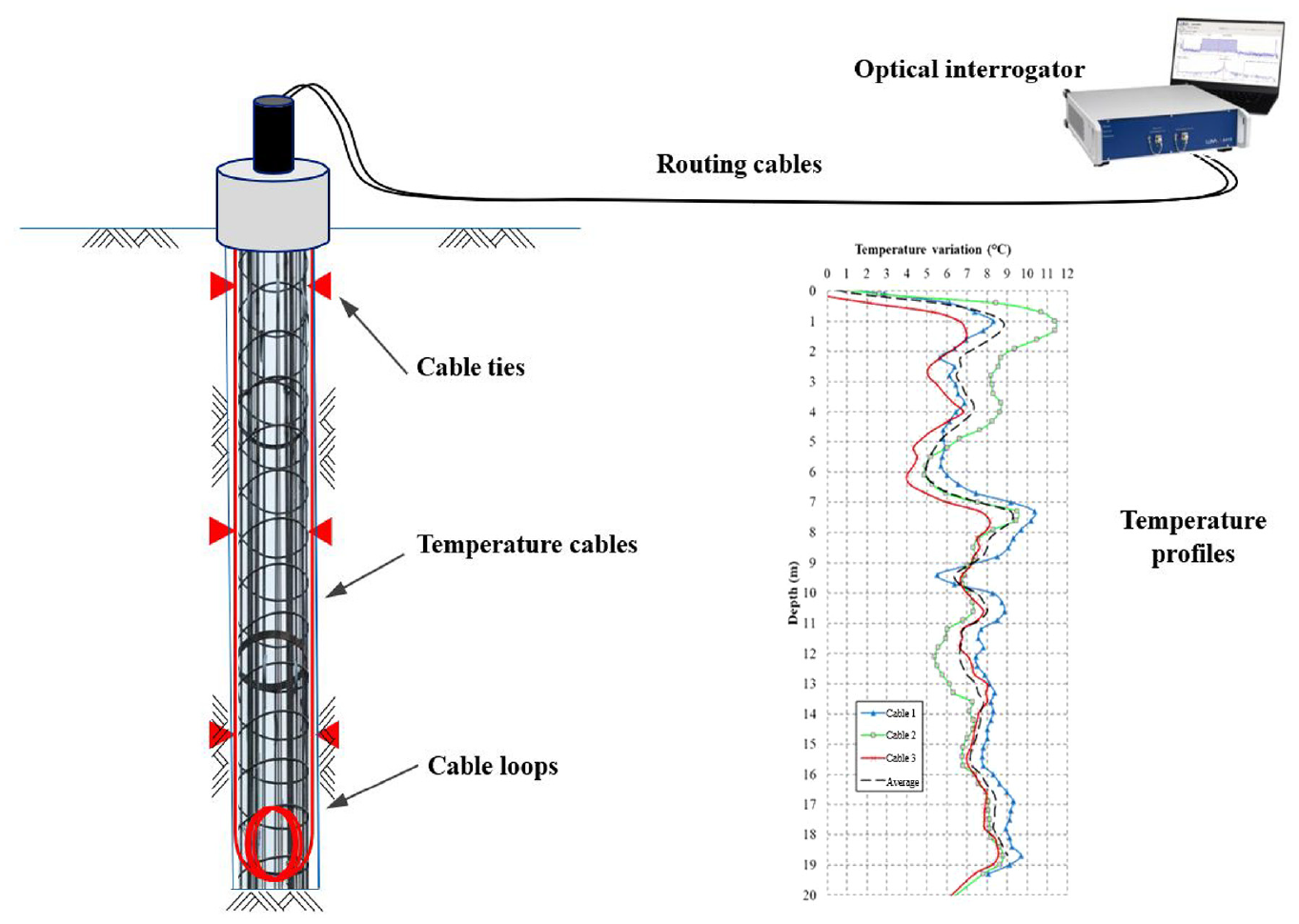
Measurement system for fibre optic sensing-based thermal integrity test.
Laboratory test
General setup
Two model piles (each 250 mm in diameter and 800 mm long) were constructed in the lab, including one control pile and one test pile with intentionally installed known defects. The laboratory testing (one pile tested at a time) was conducted at the Schofield Centre, University of Cambridge. The concrete piles were cast inside a circular metal container 800 mm in diameter and 1100 mm deep, which provided a homogeneous heat exchange on the piles’ boundaries. First, dry Hostun sand was placed inside the metal container up to a height of 800 mm; a circular steel casing (250 mm internal diameter) is then placed in the middle to retain the sand and facilitate the casting of the model pile. Instrumentation supporting frames made of glass fibre-reinforced polymer were then placed both in the sand and inside the shaft. Glass fibre reinforcement rebars have very low thermal conductivity (0.05 W/m K) and do not have a significant effect on hydration heat transfer. Fibre optic temperature sensors were attached to these glass fibre frames. The temperature data collection began around an hour before the concrete pour to precisely document the initial temperature and the thermal behaviour of fresh concrete. All fibre optic sensing cables used in this test were protected with a layer of aramid yarns and a plastic outer sheath to avoid possible damage during the concrete pour. These cables are suitable for the majority of field tests; however, another type of fibre optic cable, reinforced with steel wires, is commercially available to overcome even harsher environments if required. 29
The layouts of the test components are shown in a plan view, an elevation view and a three-dimensional view in Figure 4.
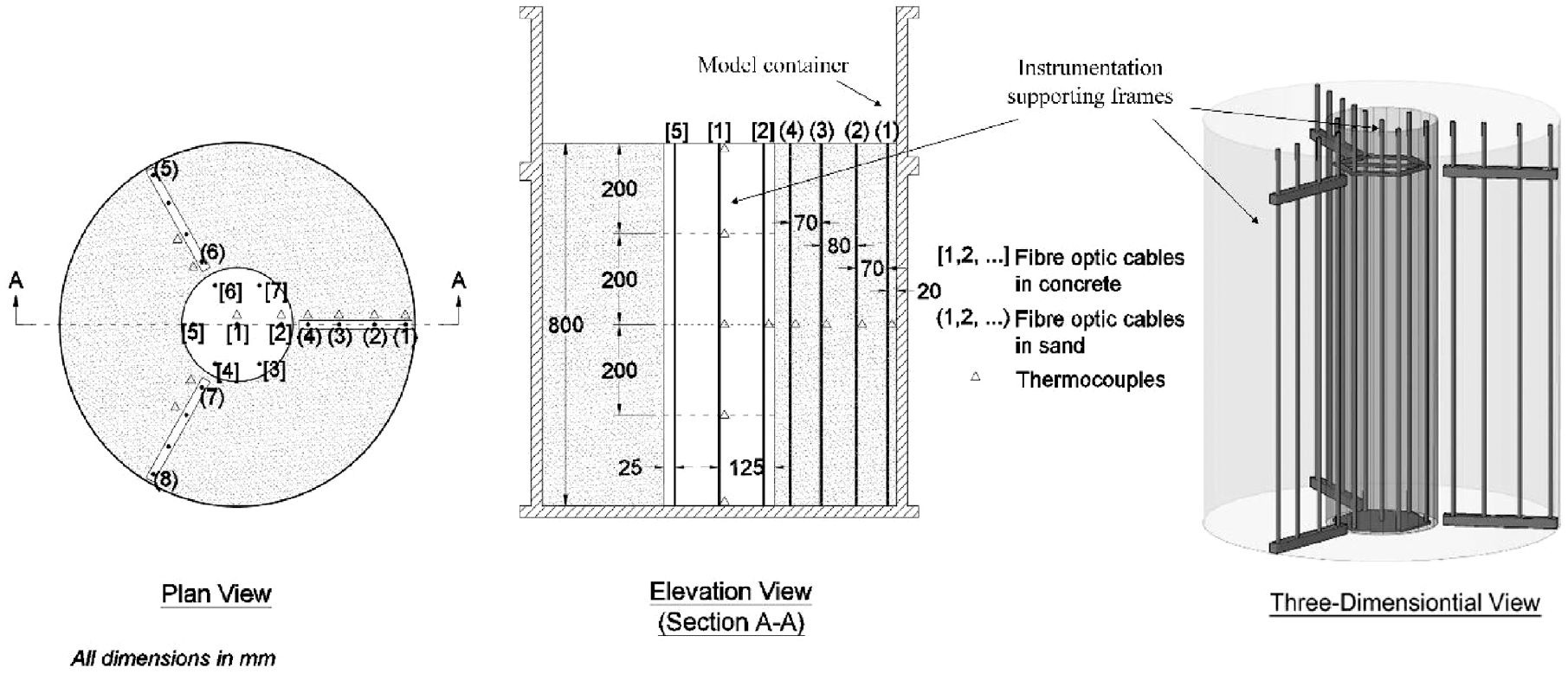
Test model: (a) plan view, (b) elevation view and (c) 3D view.
Instrumentation
The two model piles were instrumented with the Excel temperature cable (205-300 Excel OS2 4C 9/125 Loose Tube LSOH Black) in which the optical fibre cables are suspended in a gel ensuring no transfer of strain – hence, the fibres are sensitive only to temperature changes. The strain fibre optic cables (polyurethane sheath 2 mm cable) were instrumented alongside the temperature cables, the data of which, however, are not used in this paper. The cables were attached to the sensor supporting frames such that they provided measurements at eight locations in any given cross-section of the pile – six locations spaced in radial lines 60° apart (a cover of 25 mm was specified for the sensor in each radial line) and two at the centre of the cross-section. Figure 4(a) shows the configuration of the sensor instrumentation in a typical cross-section. The temperature cables were routed down, across and up the longitudinal bars starting from the central bar and travelling in a clockwise sequence around the pile until the loop was completed by running the cables back up to the central bar. This gave a total of eight cable positions for each type of cable (strain and temperature) and two complete cable loops (one temperature and one strain) in each pile. Although the length of the model piles was 800 mm, in order to avoid signal losses, the cable bends required a radius of at least 5 cm per bend. Therefore, each pile was instrumented with approximately 9.5 m of each cable, which included an extra 1 m at the start and end of each loop to allow for easier connections and manual handling. One end of each cable loop was then connected to the analyser for data collection. In this laboratory test, a sampling rate of 1 Hz and a spatial resolution of 2.6 mm were adopted.
In addition to the fibre optic cables, five thermocouples supplied by RS Components Ltd were installed in each concrete pile to measure the temperature development. Four thermocouples were attached to the central bar with a space of 200 mm from the bottom. One thermocouple was placed in the middle of the outer bar. The thermocouple measurements provided an independent measurement of temperature changes that could be compared to the fibre optic cable measurements. All thermocouples were connected to the Pico USB TC-08 data logger also supplied by RS Components Ltd. Thermocouples were also installed to collect temperature data within the sand.
The first test was designed to provide a reference – no artificial defects were included in pile one. Pile 2 in the second test was constructed with known defects. The as-built drawings of the two piles are depicted in Figure 5 and photos of them are displaced in Figure 6.
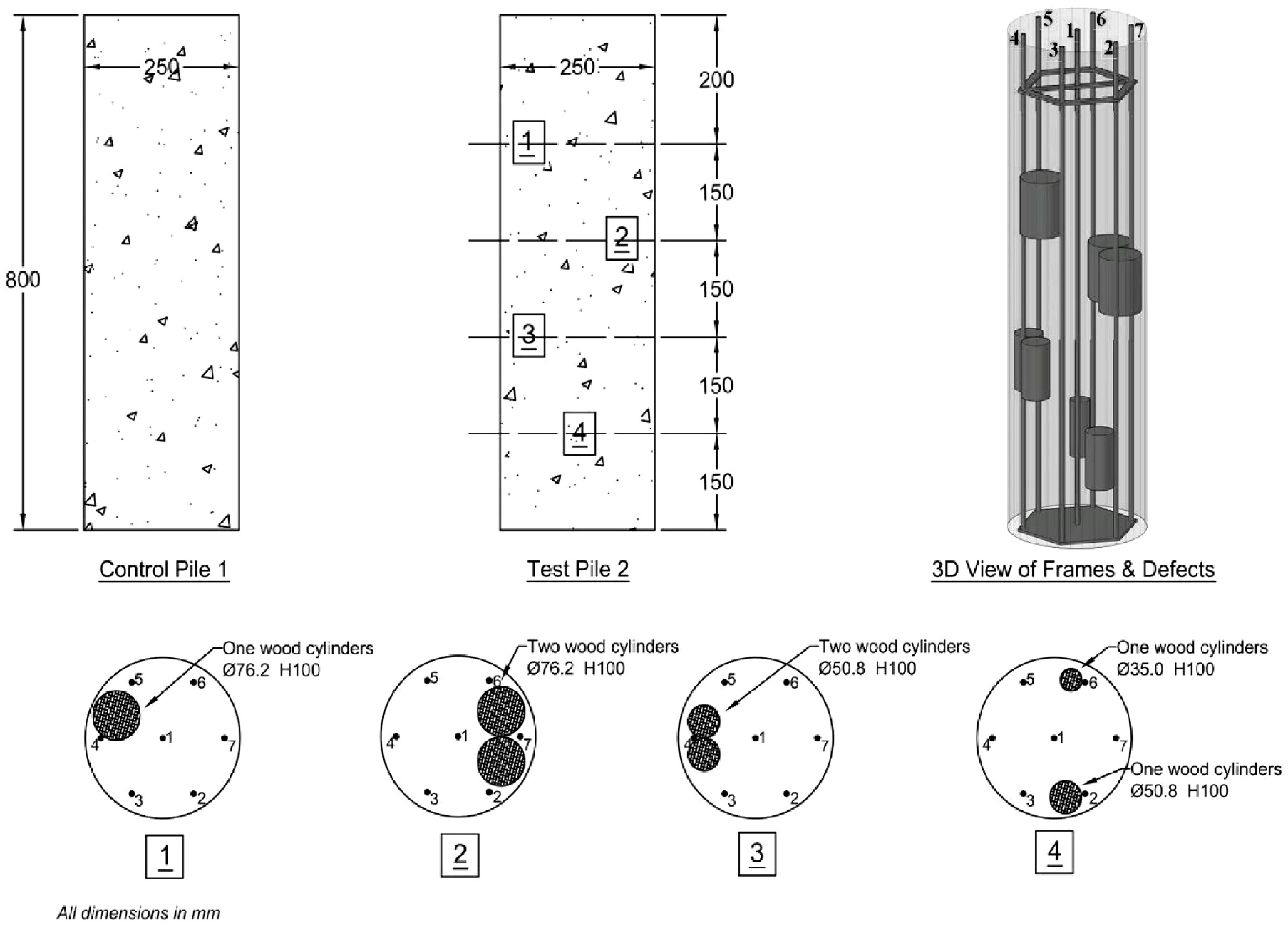
As-built piles showing locations of intentional defects.
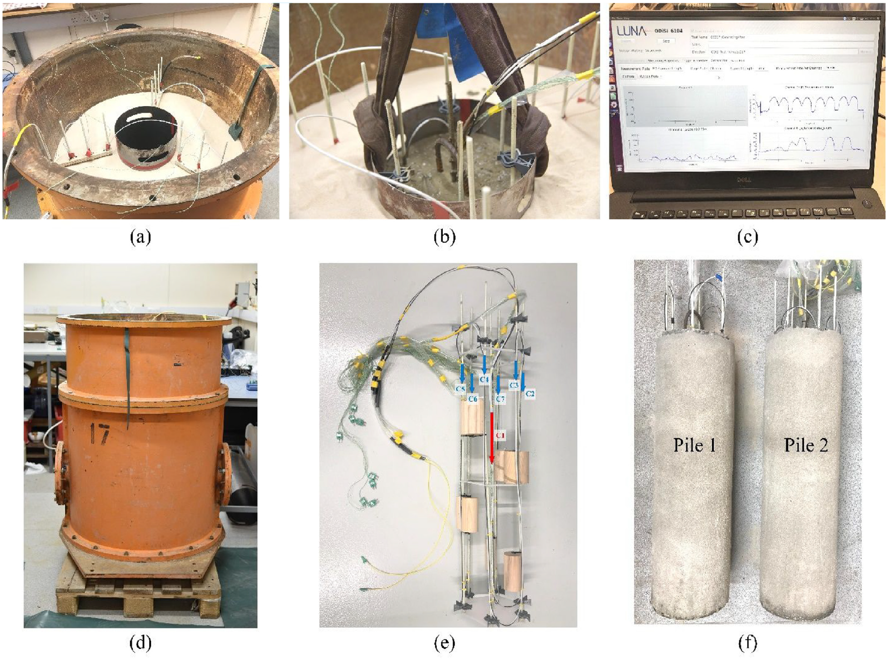
Photos for (a) model before concreting, (b) model immediately after concreting, (c) LUNA analyser, (d) model container, (e) supporting frame and fibre instrumentation and (f) as-built piles.
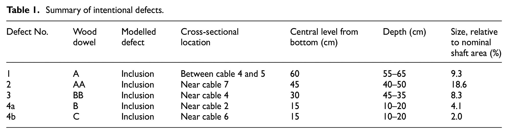
Cylindrical Ash wood dowels of three different sizes were used to simulate the defects. Type A wood dowel has a diameter of 76.2 mm, while types B and C have diameters of 50.8 and 35 mm, respectively. A total of five different defects were built in the anomalous pile (Pile 2) using the wood dowels as summarised in Table 1. The cross-sectional area of the defects is shown as a percentage of the nominal cross-sectional area of the pile. Defects 1, 4a and 4b were included to investigate defects of varying sizes adjacent to the cover of the shaft, while defects 2 and 3 (constructed using two identical wood dowels) were included to evaluate defects of different shapes and sizes. The length of all defects is 100 mm and they are fixed to the supporting frames using cable ties. To eliminate the superposition of thermals effect from adjacent defects on the temperature profiles, the inclusions were installed staggered on opposite sides of the pile with gaps of at least 50 mm in elevation.
Summary of intentional defects.
Testing procedure and concreting
During installation, a steel casing (for casting the model pile) was first placed at the centre of the model container. Sensor supporting frames for both the concrete and the sand were then installed in place. Following this, sand was poured into the model container from a fixed drop height. The sand pouring process was conducted carefully to produce homogeneous soil layers in both model piles. This could aid in the formation of consistent soil surrounding two model piles and facilitate the numerical simulation employing similar soil thermal properties. Concrete was poured at the bottom of the steel casing through a 100 mm diameter pipe (tremie) in order to avoid segregation. Using a crane at a very low speed, the steel pipe was then gradually lifted during the casting process. Care was taken to ensure the casing stayed upright during the lifting process to minimise the disturbance to the fresh concrete model pile. The photos of the pile construction process, the LUNA analyser, the model container, the supporting frame and two as-built piles are demonstrated in Figure 6.
The concrete mix (C60/70) was designed with a water-cement ratio of 0.4 and a target slump from 60 to 180 mm. No admixtures were specified. The mix design follows the UK BRE concrete design guide. 30 Details of the mix design are presented in Table 2.
Concrete mix design.
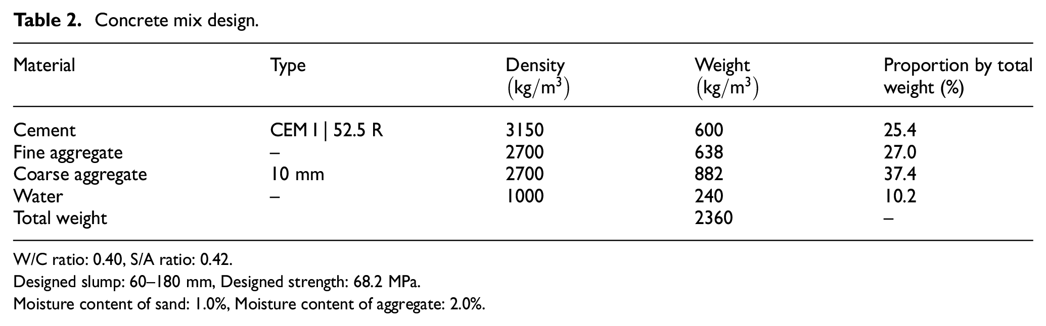
W/C ratio: 0.40, S/A ratio: 0.42.
Designed slump: 60–180 mm, Designed strength: 68.2 MPa.
Moisture content of sand: 1.0%, Moisture content of aggregate: 2.0%.
Laboratory models and field application
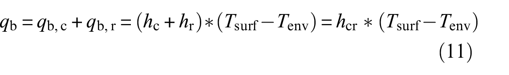
The heat transfer path and rate are determined by the pile’s geometry and boundary conditions. Figure 7(a) depicts schematically the boundary condition and heat dissipation for an idealised cast-in-place pile. Through heat conduction, the heat created by concrete curing is transported horizontally to the surrounding soil. The bottom of the shaft enables for both radial and longitudinal heat dissipation via the end. Consequently, the pile bottom temperature is typically several degrees Celsius lower than the pile body temperature. Since the top of the shaft is exposed to the surrounding environment (air), internal heat is dispersed through convection much more rapidly.
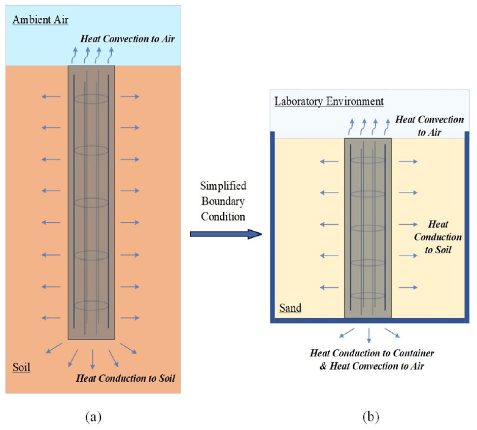
(a) Field condition and (b) Physical model
The physical model built in the laboratory is a simplified representation of the pile construction in the field. An equivalent but simplified boundary condition was designed for the lab test, which utilised two scaled-down versions of the real piles. As depicted in Figure 4(b), the primary pile body is in direct contact with sand and is therefore subject to heat conduction similar to field conditions. The circular metal container is 800 mm in diameter and the 250 mm diameter pile is placed in the centre of the model. A sufficient amount of sand in the container provides an appropriate distance (275 mm) for curing heat dissipation, which minimises the effect of the container boundary wall. In addition, the open top surface of the physical model at the laboratory permits heat convection between the concrete and air. The sole deviation from the field situation is the pile’s base, which is in direct contact with the metal container. The generated heat is initially transferred to the container by conduction before being dissipated into the environment via convection. The faster heat dissipation at the bottom in the laboratory is comparable to the faster heat transfer that occurs at the pile’s base in the field. The physical model used for this lab experiment was designed to closely resemble the field boundary conditions. Furthermore, the authors conducted a Finite Element Method (FEM) analysis to investigate the container bottom’s influence. The results showed that the laboratory boundary effect, pile in direct contact with the container at the bottom, is comparable to the field with vertical heat transfer between the pile toe and the bottom soil.
In order to quantitatively compare the scale effect of the heat transfer in the laboratory experiments to that of the full-scale piles, a Fourier number
where
Test data analysis
Pile 1 (control pile – no anomalies included)
Control pile 1 is presented as a reference for comparison purposes. The initial temperature inside the empty steel casing was 21°C. The FOS temperature development was obtained by adding this initial temperature to the temperature change data measured by the LUNA analyser. The thermocouple temperature data were directly retrieved from the associated data logger.
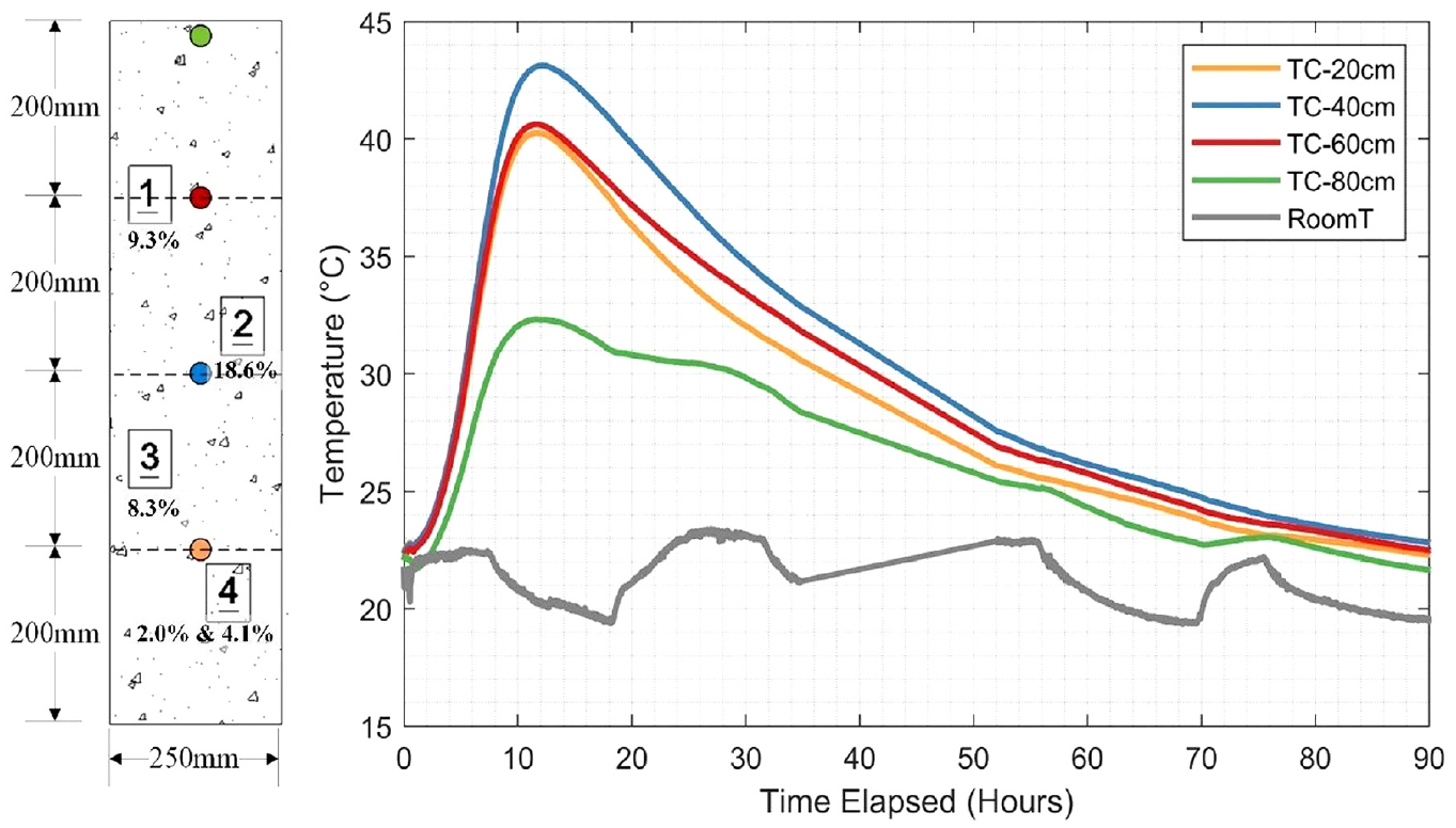
Temperature development from four different thermocouples at the centre of the pile is presented in Figure 8. The room temperature data is included in the figure for comparison purposes. A fast rate of heating was observed on the first day following concrete casting with a maximum measured temperature of 42°C at the middle of the pile approximately 11 h after the end of the concrete casing. The maximum temperatures at 20 cm depth and 60 cm depth were 2.5°C lower. The corresponding time of the maximum rate of temperature rise was approximately 7 h for the three thermocouples. After reaching the peak temperature at 11 h, the pile cooled uniformly and reached room temperature 90 h after concrete casting. Due to the temperature difference between day and night, the laboratory temperature varied between 19°C and 22°C (illustrated in Figure 8). The temperature at the pile top surface (shown in green) was significantly affected by the ambient temperature fluctuation. It should be noted that the laboratory entry door was opened accidentally at 19 h, causing an abrupt drop in ambient temperature in Figure 8.
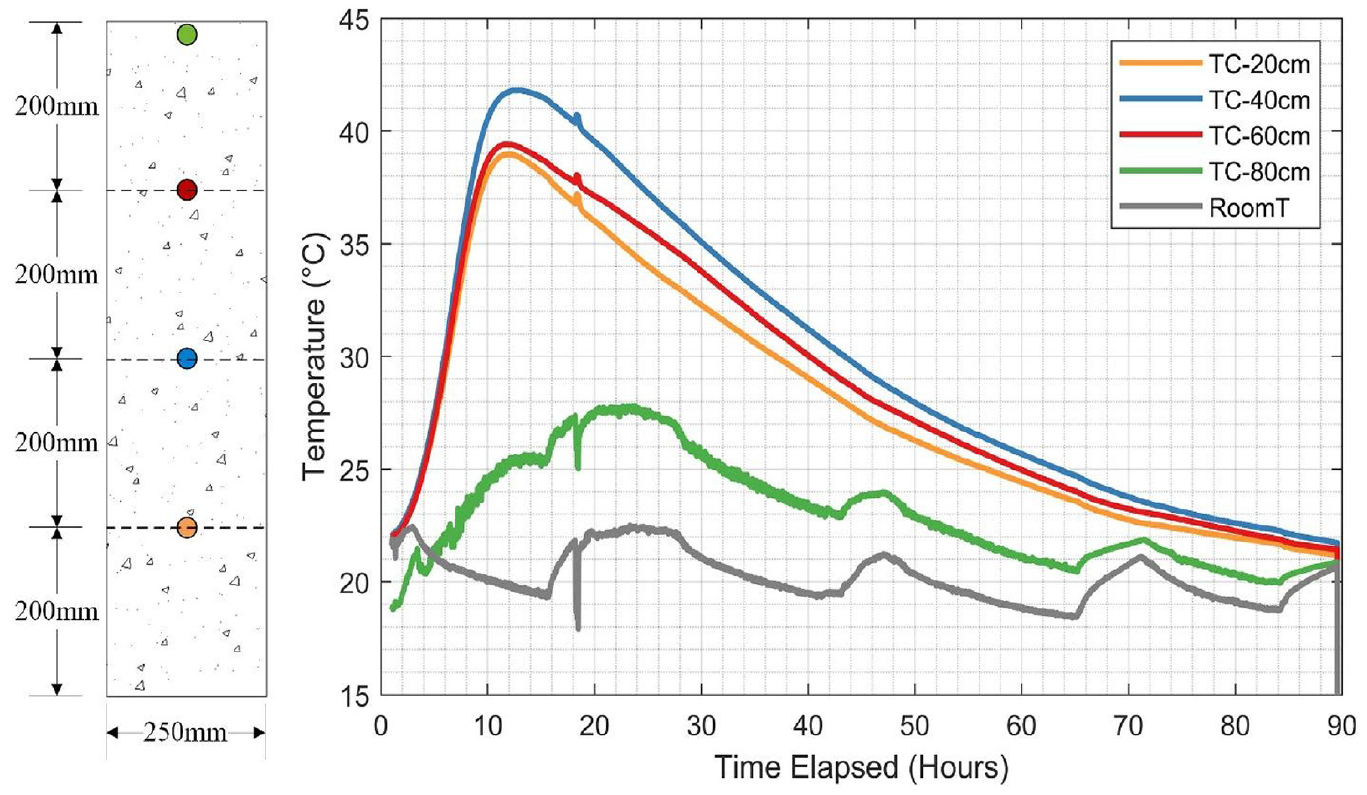
Temperature development at four sensor levels in Pile 1.
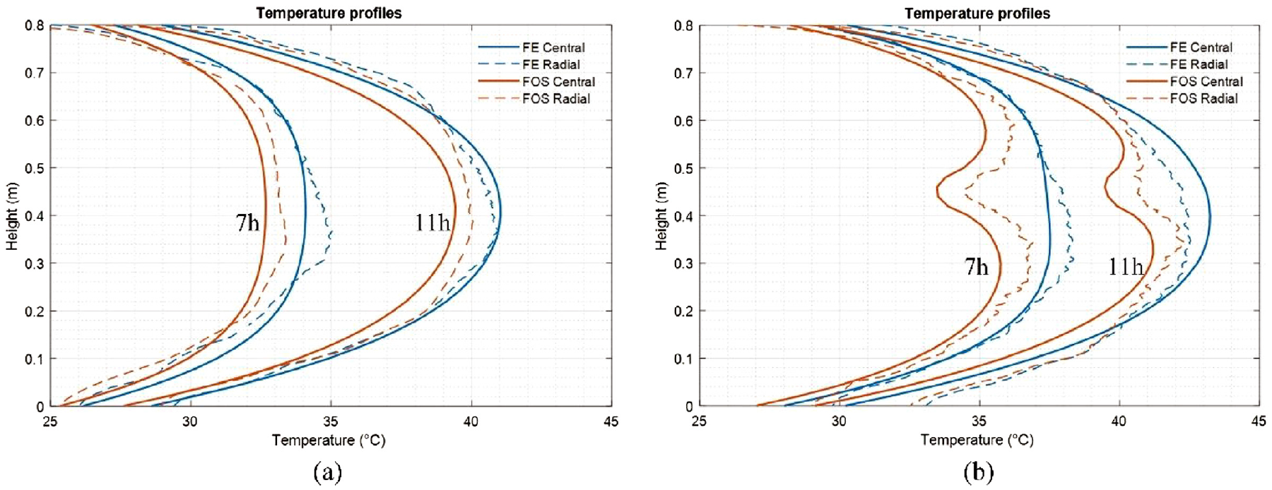
Figure 9 presents the temperature profiles at the times corresponding to the maximum rate of temperature rise (at 7 h after casting) and the peak temperature (11 h after casting). In the figures, the blue lines represent the temperature of central cable 1; the other lines show the temperature of radial cables 2–7. The central pile regions (0.3–0.5 m) heated up significantly faster and reached higher temperatures. All profiles in the figure were approximately parabolic in shape, tapering off consistently within one pile diameter (0.25 m) from the top and the bottom. The exposed top allowed faster heat dissipation than circumferential boundaries and the bottom has direct contact with the steel model container, which conducts heat at a higher rate. The temperature difference between central and radial cables was about 1°C at 11 h. Whereas such difference was more than 2°C at the time of maximum rate of temperature increase (7 h), at the pile central region (0.3–0.5 m).
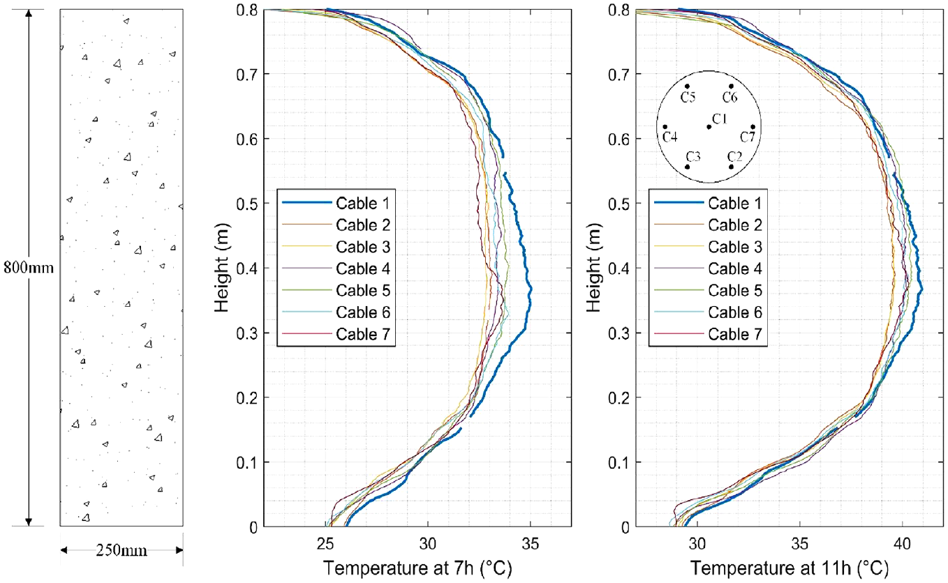
Temperature profiles at 7 and 11 h in Pile 1, including as-built pile dimensions.
Figure 10 shows thermal profiles for three sections across Pile 1 at 7 h following casting. The plots were produced by interpolating temperature data from one central cable and two radial cables at the opposite sides, namely, cable 1-2-5 for section A, cable 1-3-6 for section B and cable 1-4-7 for section C. The temperature scales were selected to emphasize the differences in cable temperature. These three interpolated thermal profiles are symmetric and consistent. The maximum temperature was achieved at the centre of the pile and the temperature gradually dropped near the concrete pile boundaries.
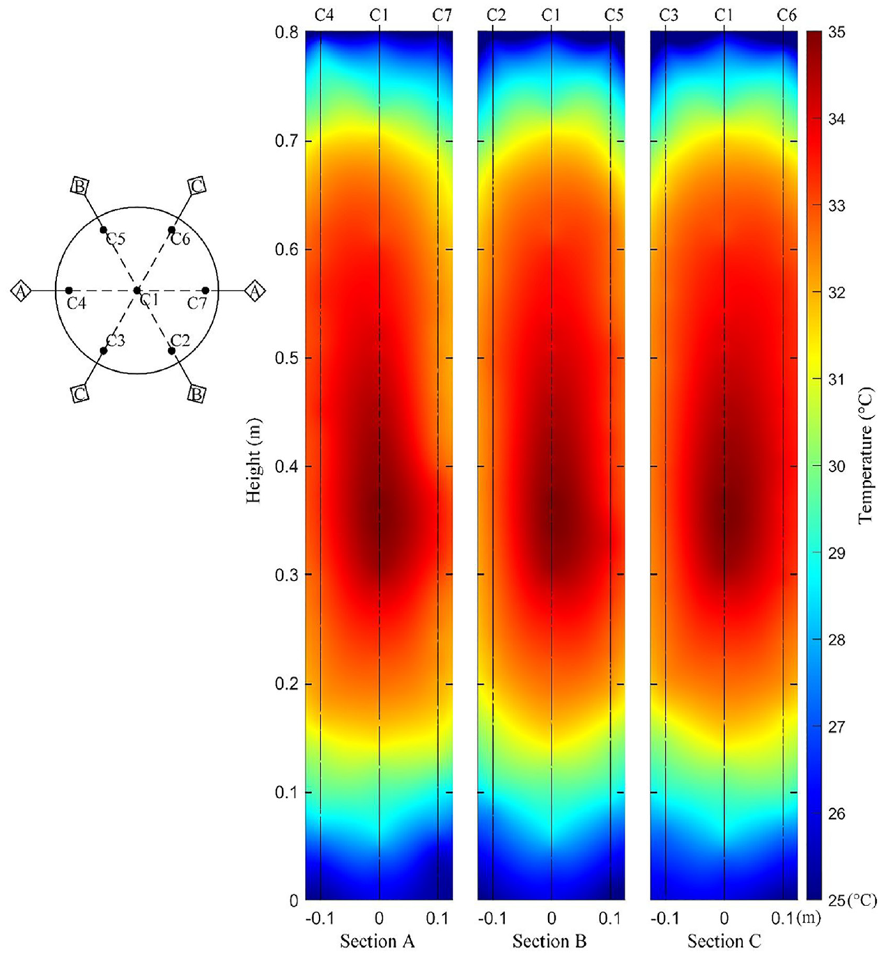
Interpolated thermal profiles at 7 h in Pile 1.
Pile 2 (engineered anomalies included)
The second test pile, Pile 2, contained intentional defects as shown in Figure 5. The dimensions, boundary conditions and the concrete mix of Pile 2 were identical to the control Pile 1. The anomalies were included to evaluate the thermal impact of defect size, location and shape. It is expected that a lower temperature should be observed on the temperature profiles close to the defects. The maximum local temperature reduction should occur near defect 2, being the largest defect occupying 18.6% of the cross-sectional area. In contrast, temperature profiles should only have a slight or even negligible decrease adjacent to defects 4a and 4b, as both take up less than 5% cross-sectional area.
The initial temperature inside the empty shaft was measured as 22°C. The temperature development versus time (data obtained from thermocouples) at four different levels is presented in Figure 11. The square boxes in the figure indicate built-in defects, whose sizes (cross-sectional area) are also illustrated below the boxes. The fastest rate of temperature increase occurred at 7 h with a peak temperature of 42.5°C reached around 11 h, 40 cm from the top of the pile. The temperature development profile in this pile resembled the control Pile 1 and no defects could be identified through this plot.
Temperature development at four sensor levels in Pile 2.
The temperature profiles of the individual cables at 7 and 11 h are presented in Figure 12. Noticeable local temperature reductions can be observed at 0.3 m (Cable 7) and 0.45 m (Cable 4) in the temperature profile plots, which could be attributed to the existence of intentional defects in these regions. The temperature decreases due to the defects are significantly more pronounced at the time corresponding to the fastest temperate increase (7 h) compared to the time of maximum temperature (11 h). This agrees with previous research (Schoen et al.)43 that the largest temperature reduction attributed to defects occurs at pre-peak times and the time of maximum rate of temperature increase could be the optimum time to assess potential defects. In the 7 h temperature profile (Figure 8(a)), the following was noted:
The temperature on cable 7 was 3°C less on average adjacent to defect 2 (located 0.45 m from the top)
The temperature on cable 4 was 2°C less on average adjacent to defect 3 (located 0.3 m from the top).
Temperature reductions due to defect 1 were less noticeable. A reduction of approximately 1°C on cable 4 at 0.6 m was noted.
Defect 4 could not be visually noted in the temperature profiles.
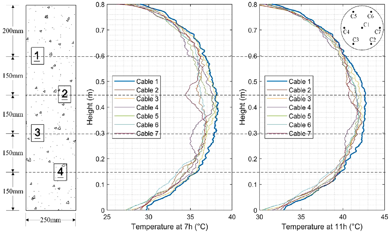
Temperature profiles: (a) at 7 h and (b) at 11 h in Pile 2.
The interpolated thermal profiles of three longitudinal sections at 7 h after concreting are shown in Figure 13. Four cross-sections (at 0.15, 0.30, 0.45 and 0.60 m) corresponding to the locations of intentional defects are plotted alongside the thermal profiles. The thermal profiles are notably different from Pile 1. In section A, three local temperature reduction regions are identified along cables 4 and 7, which correspond to the locations of defects 1, 2 and 3. Similar anomalous regions could be identified in sections B and C. However, as cables C2, C3, C5 and C6 have no direct contact with the defects, the temperature decrease is less significant. In addition, the thermal profiles are not symmetrical at the bottom close to 0.1 m height. This is caused by the presence of defects 4a and 4b near cables 2 and 6.
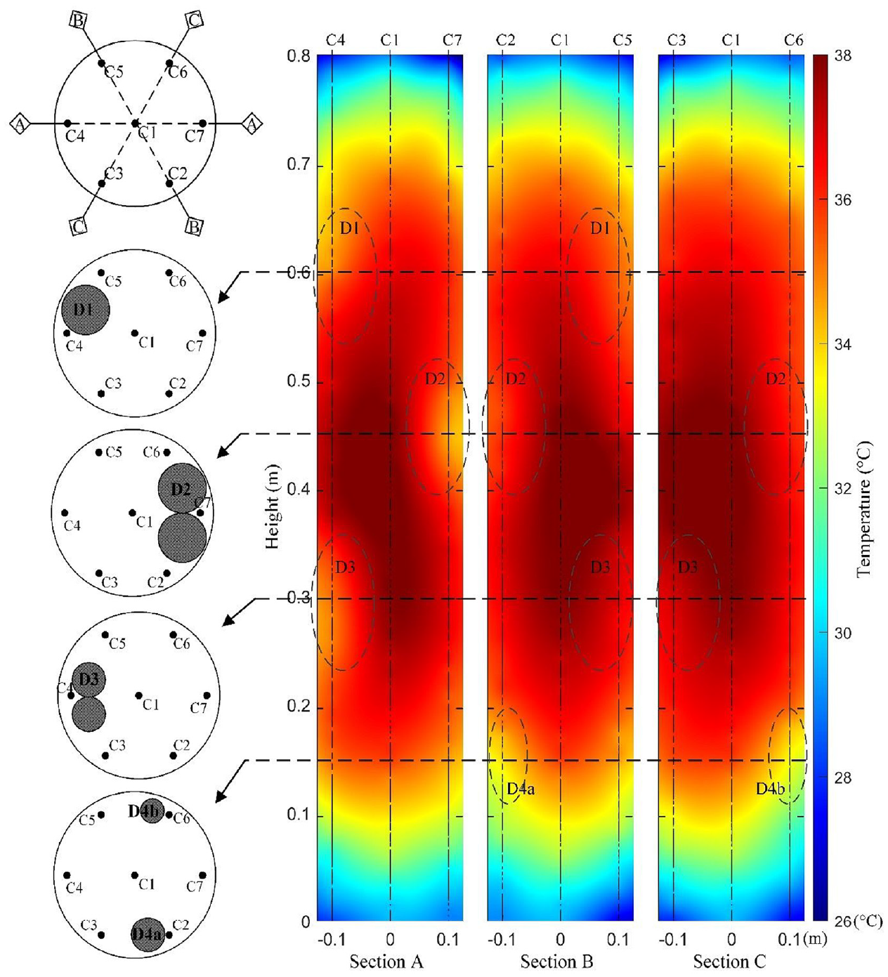
Interpolated thermal profiles at 11 h in Pile 2.
These observations suggest that interpolated thermal profiles could be a useful tool to identify possible defects. It provides more intuitive information than temperature profiles. Analysis of temperature distributions along longitudinal sections could potentially improve the detectability of defects. However, two prerequisites are essential: (1) a central cable must be installed, (2) an even number of radial cables is required. These requirements could have practical considerations that need to be taken into account.
Optimum time and defect thermal impact
The temperature profiles and thermal profiles plotted in Figures 8 and 9 shows local temperature reductions at defect locations. In order to assess the thermal influence of each individual defect, the temperature measurements near these defects need to be compared against a baseline temperature profile.
From the control Pile 1 (no defects), the temperature profiles in Figure 9 have a parabolic shape. As the boundary conditions are the same for test Pile 2, its temperature distribution on all cables along the shaft depth in Figure 12 also resembles a parabola except adjacent and at the regions of the built-in defects. Therefore, a parabolic-shaped temperature profile without defects could be fitted using the temperature data away from the defect locations. This fitted parabolic-shaped profile then serves as the ‘baseline’.
Figures 14 and 15 demonstrate two examples for obtaining the fitted baseline profiles for cables 4 and 7 in test Pile 2. As cable 7 is adjacent to the largest defect 2 (0.4–0.5 m), the raw data from 0.32 to 0.58 m were removed. Similarly, raw data from 0.2–0.4 m to 0.5–0.7 m, corresponding to defects 1 and 3, were removed for cable 4. To eliminate the boundary effect, data within the top and bottom 2.5 cm were also not used. The remaining temperature data were then employed to fit the baseline profiles through fourth-order polynomial regression. As raw data in central regions of Pile 1 without defects were relatively smooth, the second- and third-order polynomials tend to produce higher temperatures in this region. On the other hand, higher-order regression may lead to overfitting. From the fitted baseline profiles at 7 h, the defect-induced temperature reductions
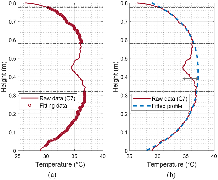
Temperature on cable 7 at 7 h: (a) profile from raw data and (b) fitted profile.
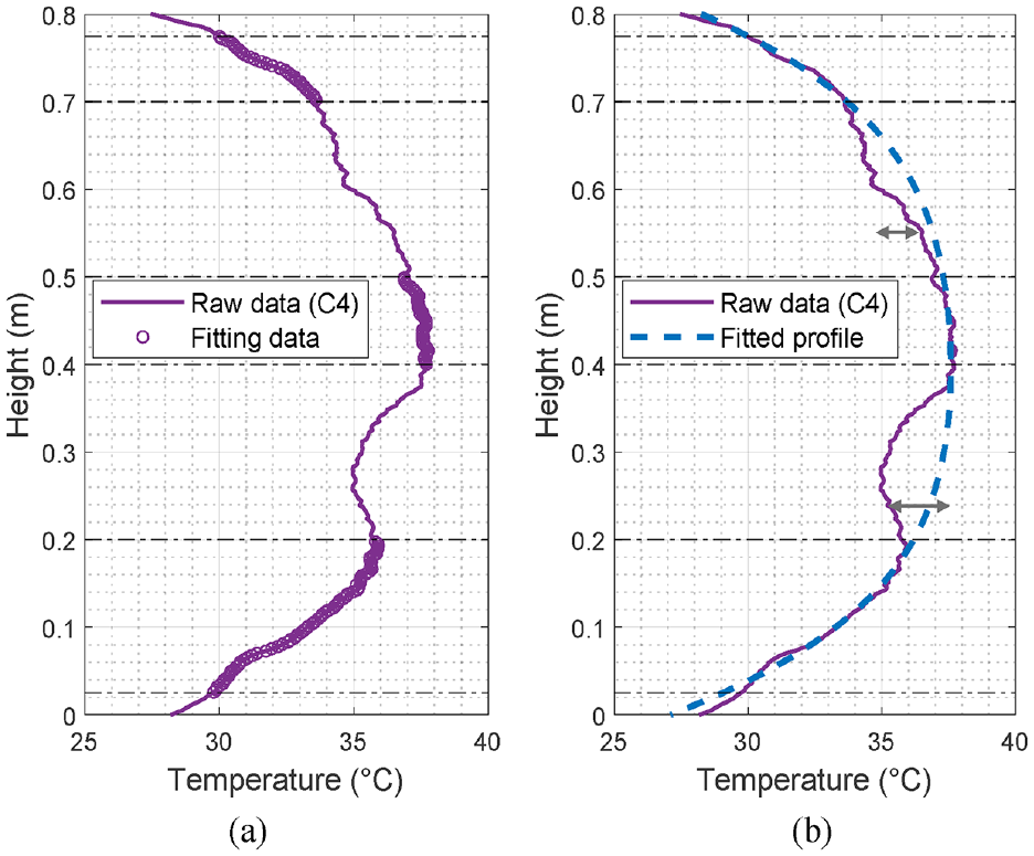
Temperature on cable 4 at 7 h: (a) profile from raw data and (b) fitted profile.
To evaluate the thermal impact of defects during the hydration process, temperature versus time graphs were created at the central level of each defect as shown in Figure 16. The temperature-time records are presented in solid lines on the left vertical axis and temperature differences
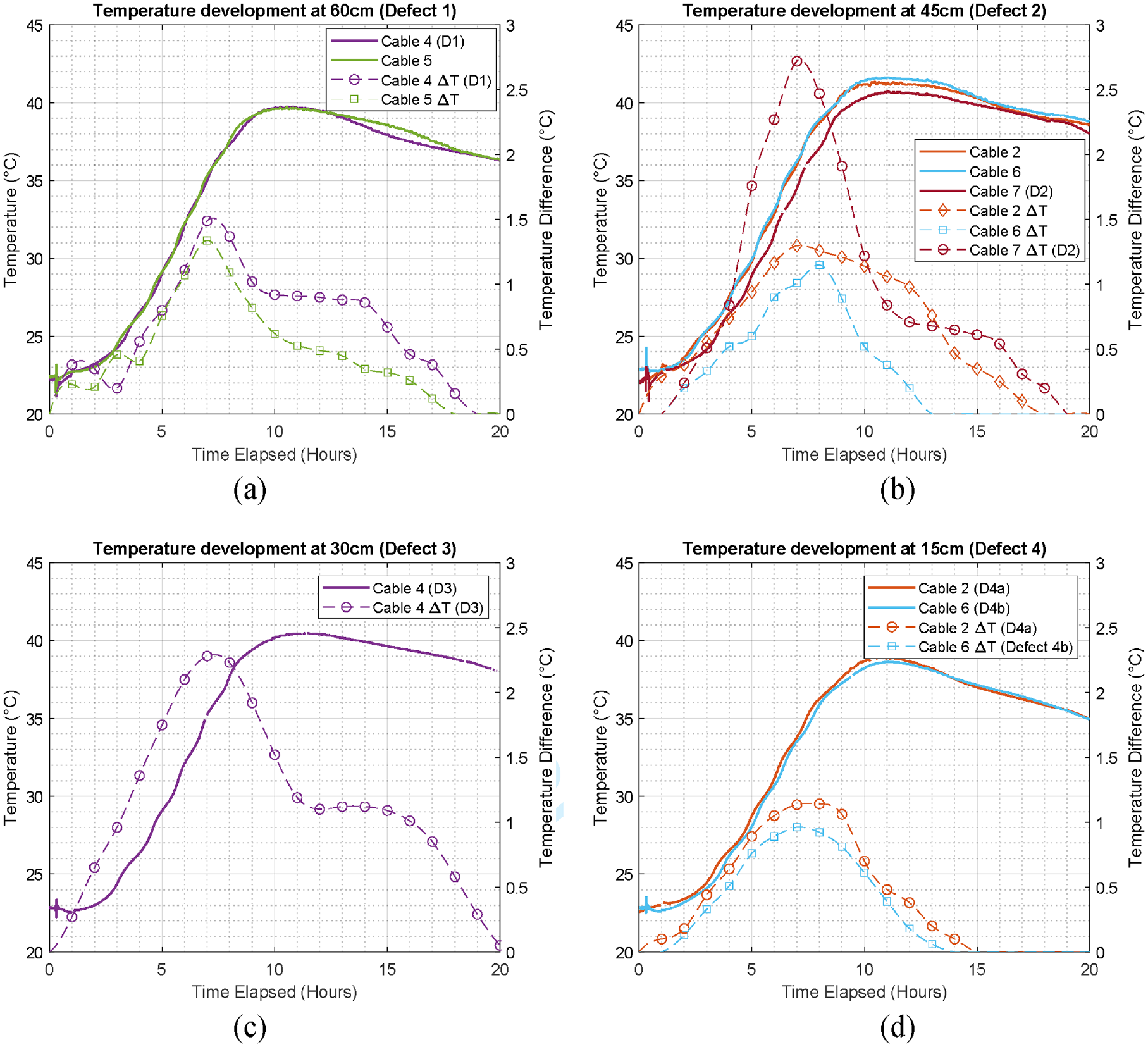
Temperature versus time at locations of (a) defect 1, (b) defect 2, (c) defect 3 and (d) defect 4.
For each defect, the largest temperature differences
The tendency for the greatest temperature difference to occur at the time of maximum rate of temperature increase (approximately 60% of the time required to reach peak temperature) is consistent. The time to peak temperature can be obtained by plotting temperature development graphs (Figures 8 and 11). This observation has considerable practical implications for the optimum time to analyse potential defects. The observation also leads to the conclusion that the thermal influence of defects is significantly more pronounced at this time point.
The maximum temperature difference on each cable caused by five defects is summarised in Table 3. Those cables that are not affected by defects are marked by a endash ‘–’. The distance between the defect centroid and the closest cable is also listed in the table. Defect 2 (18.6% of the cross-sectional area in size) had a notable thermal influence on the three nearby cables. The temperature reductions on cables 2, 6 and 7 caused by defect 2 were all over 1°C. Defect 3 has a similar shape but a smaller cross-sectional area (8.3%). Its thermal influence also extended to the three nearby cables, however temperature reductions in cables 2 and 3 are less pronounced. Defects 1, 4a and 4b consisted of one single wood dowel each. Defect 1 was located between cables 4 and 5. It resulted in a temperature reduction of around 1.4°C in both cables. Both defects 4a and 4b were less than 5% cross-sectional area with minimal corresponding thermal influence.
Summary of defect-induced temperature differences.
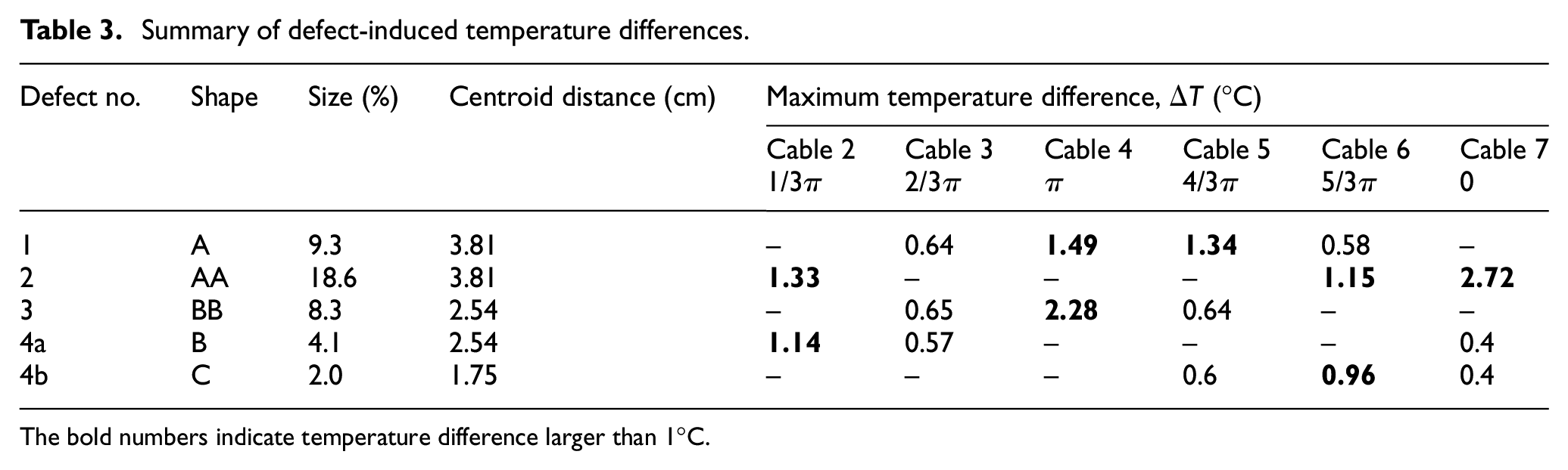
The bold numbers indicate temperature difference larger than 1°C.
Figure 17 plots the relationship between the defect size and the corresponding temperature reduction (impact) at the time corresponding to the maximum rate of temperature increase. From the experiment data, a linear relation could be fitted for the different defect shapes. From the measured temperature data, the FOS sensor sensitivity is 0.0427°C per % size of the defect and 0.0716°C per % size of the defect for double- and single-shaped defects, respectively. However, it has to be noted that the results presented in Figure 17 are not only a function of the shape and size of the defects but also the thermal property of the material of the defects. However, the plot is useful in showing the impact of the presence of the different defects on the sensors. Moreover, the results shown are also for defects, which are in direct contact with the sensing cables. In reality, there is no guarantee that the defects would be located in direct contact with a sensor and it is not practical to have a very large number of temperature measurements in each cross-section. This highlights the need to have a better understanding of the thermal zone of influence of these defects. This will enable practitioners to make informed judgments in relation to the number of sensors required and the size of the defect (hence the associated risks) that needs to be captured. This will be covered in the next section.
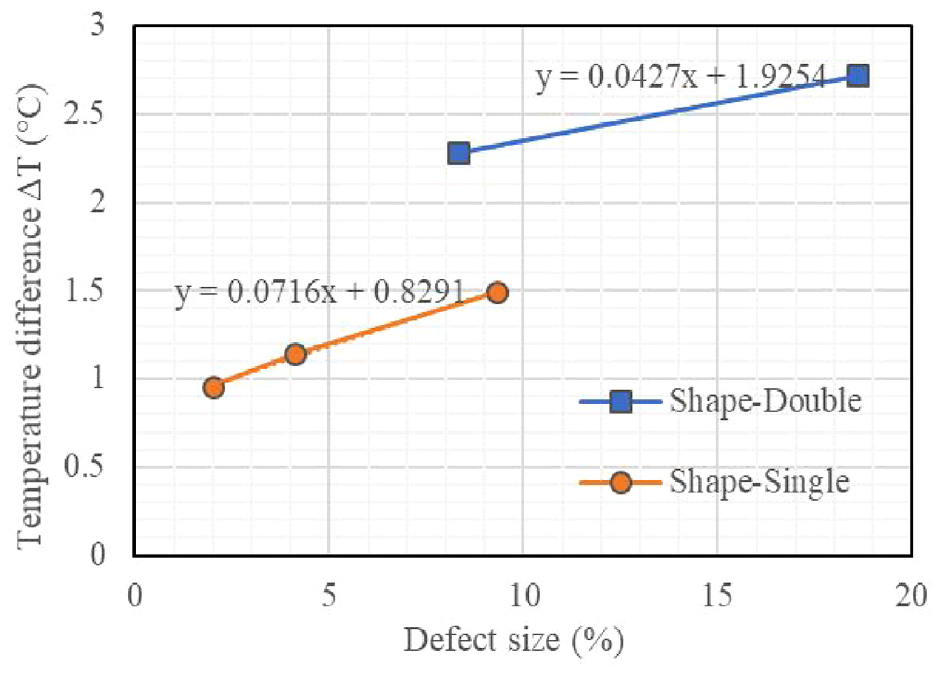
Relationship between defect size and temperature difference.
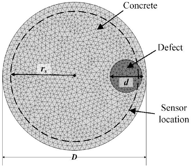
Defect zone of influence, minimum detectable size optimum layout of instrumentation
In order to make an attempt to quantify the zone of influence of the five defects and the minimum number of required cables, it is assumed that the defect-induced temperature reductions follow a Gaussian distribution – the further you move away from the centroid of the defect (in a radial direction) the smaller the temperature reduction. Therefore, the temperature difference
where
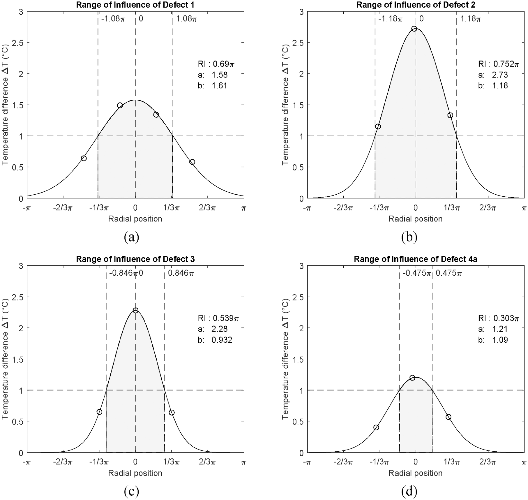
Range of thermal influence of each defect: (a) Defect 1, (b) Defect 2, (c) Defect 3, and (d) Defect 4.
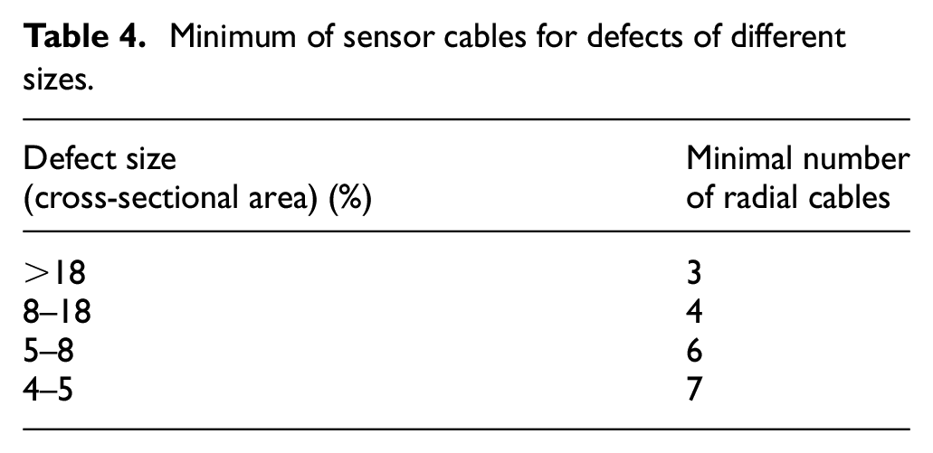
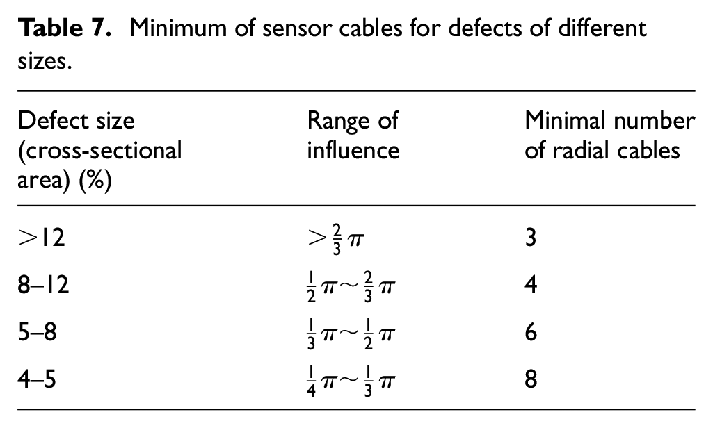
Minimum of sensor cables for defects of different sizes.
Numerical simulation
In order to verify the results obtained in the previous section, three-dimensional finite element (FE) models were developed to simulate the hydration process of the two test piles. The fundamental law governing heat conduction is commonly referred to as the principle of conservation of energy. Combined with the Fourier’s law of heat conduction, the general transient heat conduction equation can be expressed as follows:
where
Following standard procedures in the FEM, the temperature variable
Through applying the Galerkin weighted residual method over domain Ω, the governing equation can be expressed in integral form:
A matrix format more convenient for numerical implementation can be written below:

where the elemental matrices and vectors are computed through:
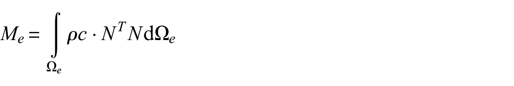
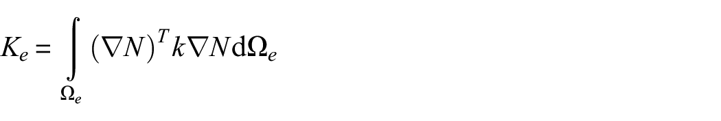
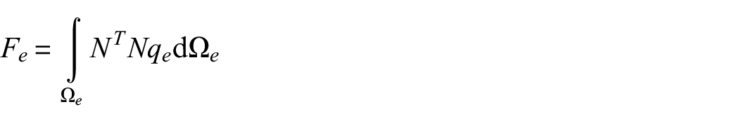
To discretize the problem fully implicitly, the partial derivative of temperature with respect to time
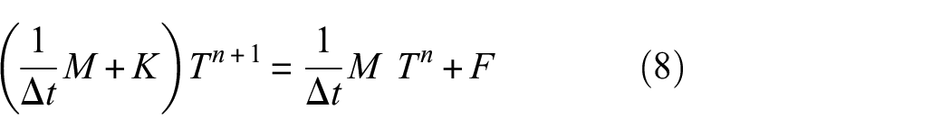
The FEM program was developed in MATLAB following the above procedure. The geometry of the FE model was exactly the same as the as-built piles. Four-node tetrahedral mesh elements were used in the FE discretization. A full-scale model containing the concrete piles, the sand, the steel container and the designed defects is shown in Figure 19. The average element sizes for concrete and soil were 1 and 8 cm respectively. Elements in the concrete should be sufficiently small to simulate the smallest designed defect, whereas elements in the soil should be sufficiently large to reduce the computational time.
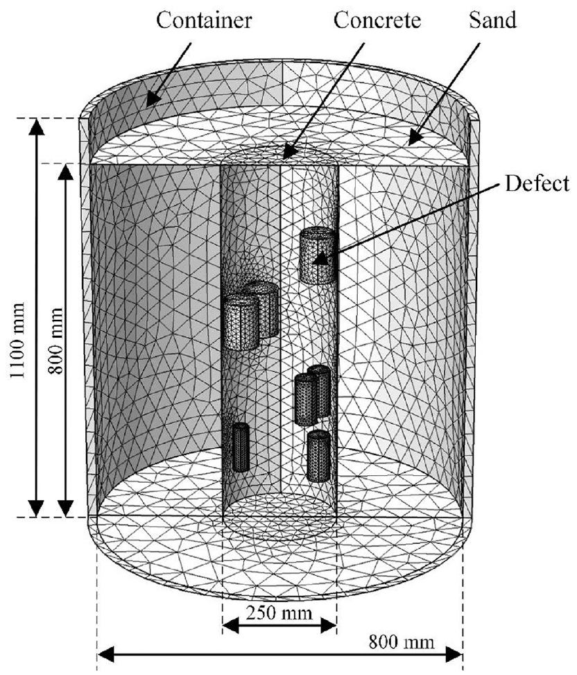
Tetrahedral mesh of the laboratory test model.
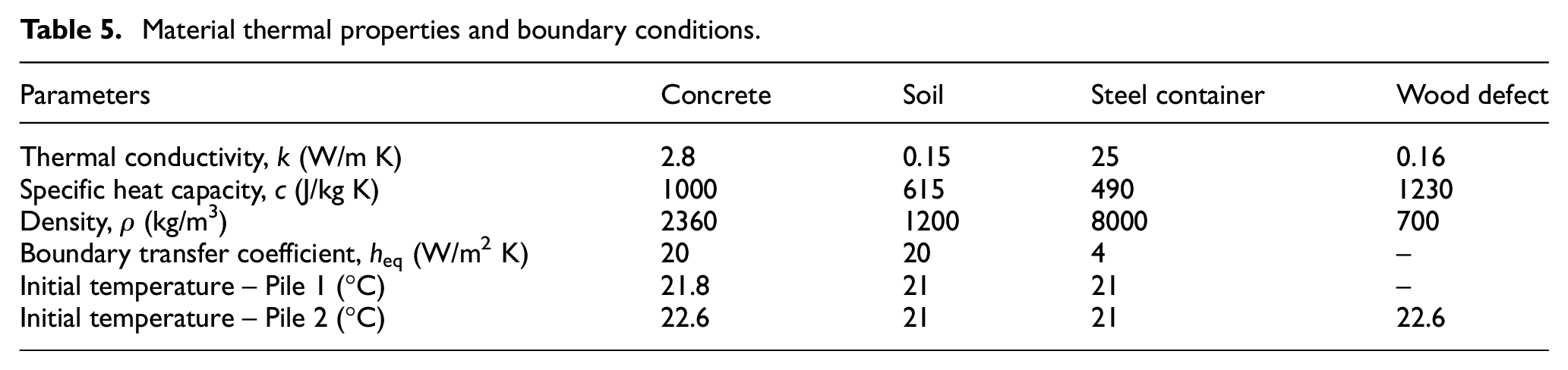
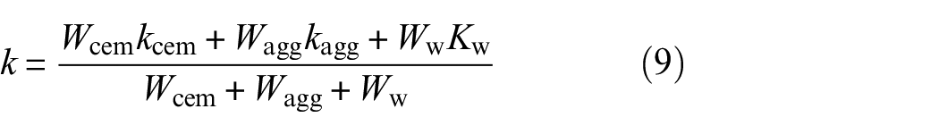
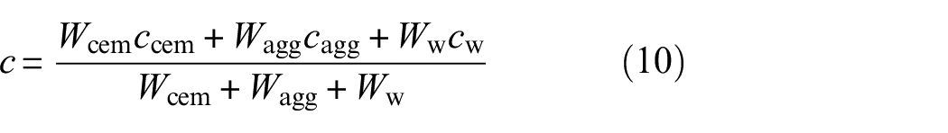
The property of each material used in the model is summarised in Table 5. Lura and Breugel
34
and Ruiz et al.
35
provide an estimation of concrete material thermal properties based on a weighted average of the components of the concrete mix as shown in Equations (9) and (10). Thus, the thermal conductivity and specific heat of concrete were accordingly calculated as 2.8 W/m K and 1000 J/kg K. The values of sand thermal parameters were chosen following Mitrani.
36
The initial temperature of each material was set to the appropriate thermocouple readings at the start of the tests. Thus, the Fourier number
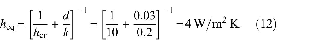
Material thermal properties and boundary conditions.
The convection heat flux
The hydration model developed by Schindler and Folliard
39
was employed in the numerical simulations. The heat generation rate
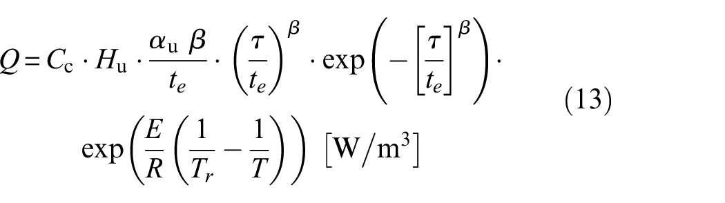
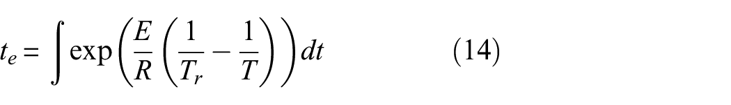
where
Hydration model parameters.
Using the material properties and the hydration parameters listed above, the temperature predictions within the entire model can be obtained through the FE modelling different stages of the hydration process. The comparison between simulated and measured temperature profiles for Pile 1 (no anomalies) and Pile 2 (with designed anomalies) is shown in Figure 20. The temperature data and the FE predictions at 7 and 11 h respectively match reasonably well.
Comparison of temperature profiles for (a) Pile 1 and (b) Pile 2.
In order to assess the zone of influence of each defect, temperature contours of four cross-sections are plotted in Figure 21. The contours are produced using 7 h FE data, when defects have the most significant thermal impact. Each row in Figure 17 corresponds to the mid-point of one of the defects – that is Figure 17(a) to (c) correspond to defect no. 1 (at 60 cm) and so on. Figure 21(a), (d), (g) and (j) (column 1) are the FE predicted temperature contours for Pile 2 (with designed defects), while Figure 21(b), (e), (h) and (k) (column 2) shows the FE predictions for Pile 1 (without defects). The temperature difference between these two predictions (with and without defects) is shown in Figure 21(c), (f), (i) and (l) (column 3). Defect 2 (18.6% area) influenced more than half of the entire cross-section and produced a maximum local temperature reduction of up to 4°C. Defects 1 and 3, which take up about 9% cross-sectional area, caused a temperature reduction over 1°C on approximately one-third of the cross-section. In comparison, the zone of influence for defect 4a (4% area) was relatively small while the influence for defect 4b (2% area) is negligible. Therefore, at least three sensing cables are required to detect defect 2, four cables are required for defects 1 and 3, eight cables for defect 4a and defect 4b cannot be identified using the current setup. These findings from the FE results agree well with the previous conclusions from the lab test data analysis.
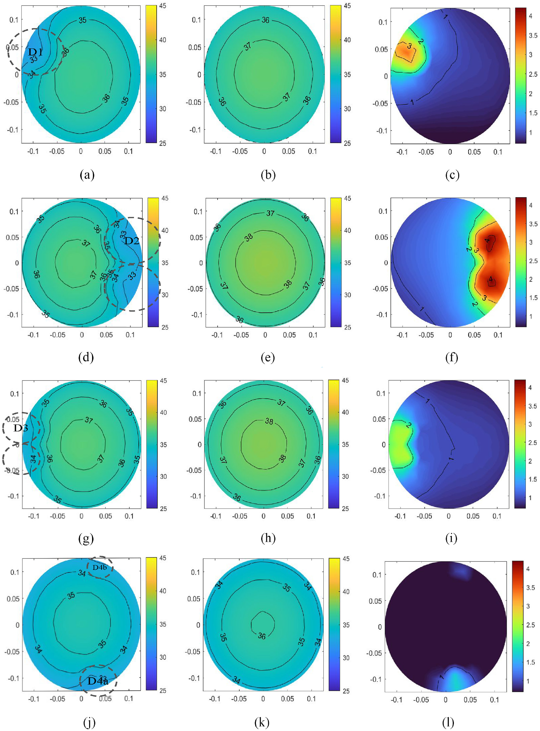
Temperature contours at 7 h.
The temperature difference contour plots (column 3 in Figure 21) have shown the RI of four test defects and give a good indication of the required number of sensor cables.
In order to generalise the above findings, four 3D FE analyses on piles of different diameters
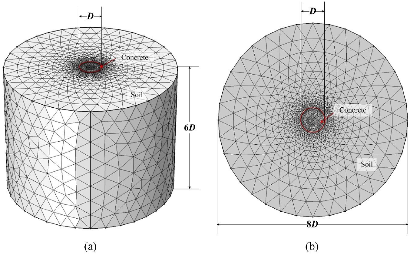
(a) Oblique view of the finite element model with the diameter and the depth of 8
The temperature development of these four models without any defects was first established from the simulations. Using these results, the time of maximum rate of temperature increase

Cross-sectional view of the finite element model at 3
The temperature development for the model (including 1% defect) was then simulated and compared to the original temperature in the model without defects. The corresponding temperature difference contours at time

Then longitudinal temperature profiles for each sensor location on a circle of
To determine the RI for defects of different sizes and to validate the number of cables required for defect detection, the following criteria were set:
The temperature reduction due to a defect on 2D cross-sectional contour plots must exceed 1°C (e.g. temperature contour in Figure 20). Smaller reductions are ignored.
Local temperature reductions on the longitudinal temperature profile must also exceed 1°C (e.g.
The first criterion ensures that the temperature reduction due to a defect is more than the minimum sensor detectable temperature. The second one ensures the defect is clearly identified from the temperature profile plots. Following the analyses above, the results are summarised in Table 7. Piles of different sizes share similar characteristics. For defects more than 12% cross-sectional area, its RI is more than
Minimum of sensor cables for defects of different sizes.
These findings suggest that thermal integrity testing has the capability to quantify the severity and distinguish the type of pile defects. Different defects will cause varying degrees of local temperature reductions and varying ranges of influence. This information can be used to back analyse the defect size and assess its nature. Recent research on thermal integrity testing5,33 has proposed a novel data interpretation framework, which integrates cement hydration model, optimisation with field temperature data and FE modelling to provide a staged risk-based approach for pile integrity assessment. Thus, thermal integrity testing could be a powerful tool in evaluating as-built pile quality on site.
Conclusion and recommendations
This article presented a laboratory thermal integrity test of two piles with and without intentional defects. The test utilised distributed FOS to monitor the temperature development of the early-age concrete. Serval important conclusions regarding the test application have been drawn based on data analysis and numerical simulation results.
The distributed fibre optic sensor system is able to capture the thermal data of cast-in-situ concrete and show localise defect-induced temperature variation. It can be an effective standalone sensor system for thermal integrity tests.
The optimum time to analyse potential defects is at pre-peak time. The defect-induced local temperature reductions are more pronounced at the time of fast rate of hydration, which is about half to two-thirds of the time of peak temperature.
The minimum defect size that can be picked up by the thermal integrity test is 4% of the cross-sectional area provided that a fibre optic sensor with a similar spatial resolution is employed. Defects with a size of less than 4% produce neglectable local temperature variations which are difficult to be distinguished from either cross-sectional temperature change contour plots or longitudinal temperature profiles.
The range of thermal influence for defects larger than 12% is about one-third of the cross-sectional area and the minimum number of required cables is three. For defects of the following sizes, 4%–5%, 5%–8% and 8%–12%, at least eight, six and four cables need to be installed on the reinforcement cage. This finding has been validated through numerical simulation for piles of different diameters with defects of various sizes. For better data analysis, an even number of temperature cables is preferred.
These conclusions addressed the foundational questions regarding the proper data analysis time, the optimum sensor deployment strategy and the corresponding defect detectability. The defect-induced local temperature reduction is more pronounced at the time of the fastest temperature increase. The evaluation of longitudinal temperature profiles at this time can significantly improve the test results. The study also established a relationship between test detectability and number of sensor cables. Depending on the required accuracy and the maximum acceptable defect size of each specific project, engineers can design the most efficient sensor deployment plan. These conclusions provide practitioners with a guideline for on-site tests and data evaluation. With a standardised test practice and a comprehensive understanding of the test capability, the thermal integrity test will become a promising integrity test method in the piling industry.
Footnotes
Acknowledgements
The authors thank Mr Chris Barker (Ove Arup and Partners Ltd) and Mr Anthony Fisher (Cementation Skanska Ltd) for their expertise and support throughout all aspects of the study.
Declaration of conflicting interests
The author(s) declared no potential conflicts of interest with respect to the research, authorship, and/or publication of this article.
Funding
The author(s) disclosed receipt of the following financial support for the research, authorship, and/or publication of this article: This research has received support from the Centre for Digital Built Britain (CDBB) at the University of Cambridge which is within the Construction Innovation Hub and is funded by UK Research and Innovation through the Industrial Strategy Fund. This work is also performed in the framework of ITN-FINESSE, funded by the European Union’s Horizon 2020 research and innovation program under the Marie Skłodowska-Curie Action grant agreement no. 722509.