Thermal integrity testing of cast in situ piles: An alternative interpretation approach

Abstract

Integrity testing of deep cast in situ concrete foundations is challenging due to the intrinsic nature of how these foundations are formed. Several integrity test methods have been developed and are well established, but each of these have strengths and weaknesses. A relatively recent integrity testing method is thermal integrity testing. The fundamental feature is the early age concrete release of heat during curing; anomalies such as voids, necking, bulging and/or soil intrusion inside the concrete body result in local temperature variations. Temperature sensors installed on the reinforcement cage collect detailed temperature data along the entire pile during concrete curing to allow empirical identification of these temperature variations. This article investigates a new approach to the interpretation of the temperature variations from thermal integrity testing of cast in situ concrete piles and presents a field case study of this approach. The approach uses the heat of hydration and heat transfer theory and employs numerical modelling using the finite element method. The finite element model can be customised for different concrete mixes and pile geometries. The predicted temperature profile from the numerical model is then compared, in a systematic manner, to the field test temperature data. Any temperature discrepancies indicate potential anomalies of the pile structure. The proposed new interpretation approach could potentially reduce construction costs and increase the anomaly detection accuracy compared to traditional interpretation methods.

Introduction

The deep foundation industry is increasingly constructing larger and deeper foundations to support taller buildings, structures with larger spans and buildings in poor ground conditions. While the machinery is continuously developing, construction of such large and deep foundations is not without its challenges. In addition, it is reasonable to expect that foundation reuse will increase in future as records are better kept.

The integrity and quality of these cast in situ foundation piles present significant challenges to the engineering profession. In recent years, pile repair and the associated maintenance accounted for a significant part of the construction cost. In the United Kingdom, infrastructure repair and maintenance costs account approximately to £15 billion each year – a fifth of the total construction costs. ¹ It is therefore crucial to ensure the pile quality at the construction stage. However, the intrinsic nature of these underground structures (limited accessibility, low visibility, large depth, etc.) adds considerable difficulties to structural quality inspection.^2,3

Anomalies present in deep foundations – for example, voids, soil intrusions, material loss or shaft collapse – could result in structure instability and/or severe durability issues. It is reported that among 10,000 tested bored piles in the United States and Germany, more than 15% of pile test results showed signs of minor defect signs and 5% of tested piles were confirmed with major defects.^4–6 These defects can have significant financial implications and cause construction programme delays, as the evaluation of the pile bearing capacity, serviceability and structural safety is dependent on the knowledge of any existing pile anomalies. It is imperative that any construction defects are identified at an early stage, particularly when piles are heavily loaded. However, without adequate monitoring techniques and appropriate identification methods, these defects could very easily go undetected. Thus, testing techniques for the integrity of bored piles are of great value to foundation construction. To address this problem, research works have carried out a great deal of work to understand underground structure load transfer mechanisms as well as the temperature and strain response of these underground structures using various methods.^7–9 Traditional integrity testing methods – including sonic pulse echo (SE) testing, crosshole sonic logging (CSL) and gamma-gamma logging (GGL) – are widely used to assess the risk of these geotechnical structures.

However, the limitations of these methods are also obvious. In the SE testing method, the maximum depth is limited by the presence of stiff soil or rock, a pile Length/Diameter (L/D) ratio of 20, and it can be difficult to distinguish the soil response from the pile response. In the CSL and GGL testing methods, the connection of long access tubes is a risky activity, and even then only a limited volume of concrete between/around the access tubes can be assessed.

Recently, a new integrity test called thermal integrity profiling (TIP) has been put into use in foundation construction. It measures temperature changes and thermal profiles of concrete during curing. Heat generation and dissipation of early age concrete is determined by the concrete mix, the ground conditions and the geometry of the concrete structure. If defects exist inside the concrete body, they will result in local temperature variations when compared to the expected heat generated during curing. ¹⁰ When this method is employed on a circular concrete pile, a local reduction of temperature indicates concrete material loss and is directly interpreted as a reduction in the pile diameter. Inversely, an increase in temperature suggests that a bulge has occurred. Furthermore, the method can also be used to assess the steel reinforcement cage alignment within the shaft since an off-centre cage will exhibit higher and lower temperatures on opposite sides of the shaft. ¹¹

This new technique of TIP, like other integrity testing methods, also has its limitations. The current industry data interpretation practice is primarily based on empirical experience. Anomaly detection through direct analysis of temperature profiles is currently indicative or suggestive, and short of extracting the pile, it is difficult to verify whether the interpretation is valid or not. Temperature signatures are usually similar, and the potential numerous causes are not easily isolated. Moreover, the hydration process and temperature signatures vary with cement composition and the pile boundary conditions. The use of pile construction logs and concrete yield data in the TIP analysis for predicting pile radii along the shaft has been proposed by a number of researchers.^12–14 In this interpretation method, the overall average temperature of the pile is used as a reference; measurements which are cooler than the overall average are areas of reduced concrete volume (or poor concrete quality) and areas with a higher temperature than the average are areas of increased concrete volume. The method translates the temperature variations from the overall average to changes in pile geometry; while this is a good starting point, it is obviously a simplification of the reality. In addition, the existence of anomalies within the pile will affect the overall average temperature, the reference used to identify problematic regions. Chunge ¹⁵ conducted a number of laboratory experiments where he took detailed temperature measurements from concrete columns (with and without known inclusions representing anomalies) following casting and concluded that the method of analysing temperature profiles may have the potential to locate anomalies but not necessarily identify their nature or geometry. His experimental findings highlighted the complexity of empirically translating temperature measurements to pile geometry and question the level of accuracy with the current TIP interpretation approach. He reported that ‘there are numerous causes for ambiguity that are not easily isolated and several factors that produce similar behaviour’. ¹⁵ As such, an improvement to this approach is needed.

This article presents a case study of a TIP test carried out on a cast in situ concrete pile in East London. The original data interpretation method is improved using a numerical model to identify the pile defect location and size. The finite element method (FEM) is employed to model the cement hydration and heat transfer process within the concrete body and the soil. The model can predict temperature development of the early age concrete with and without anomalies. Combining both numerical results and testing data, the integrity of the test pile is systematically evaluated with improved accuracy.

Test site and instrumentation

This East London project involved the construction and monitoring of an offline test continuous flight auger (CFA) pile. Due to the limited experience with thermal integrity testing in the United Kingdom, it was necessary to trial the effectiveness of the method. The offline test pile was constructed in June 2015 in order to validate the integrity testing methods proposed for the test piles. The design length of the CFA pile was 20 m with a nominal diameter of 900 mm and a reinforcement cage diameter of 750 mm. The reinforcement cage was attached with thermal wire cables (TIP-1, TIP-2 and TIP-3 as shown in Figure 1) as it was plunged into the shaft. During curing, the cables were connected to a Thermal Acquisition Port (TAP), and temperature was measured at 300 mm intervals along the pile every 15 min. The pile was installed through layers of clay, sand and gravel as shown in Table 1. The upper groundwater level was at the top of the River Terrace Deposits. The Upnor Formation and Thanet Sand strata were under-drained with the lower groundwater level at 27.0 m depth.

Figure 1.

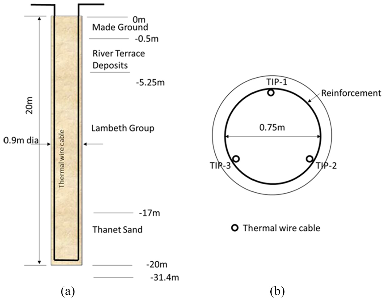
Geometry and instrumentation of the test pile: (a) plan view and (b) cross-section.

Table 1.

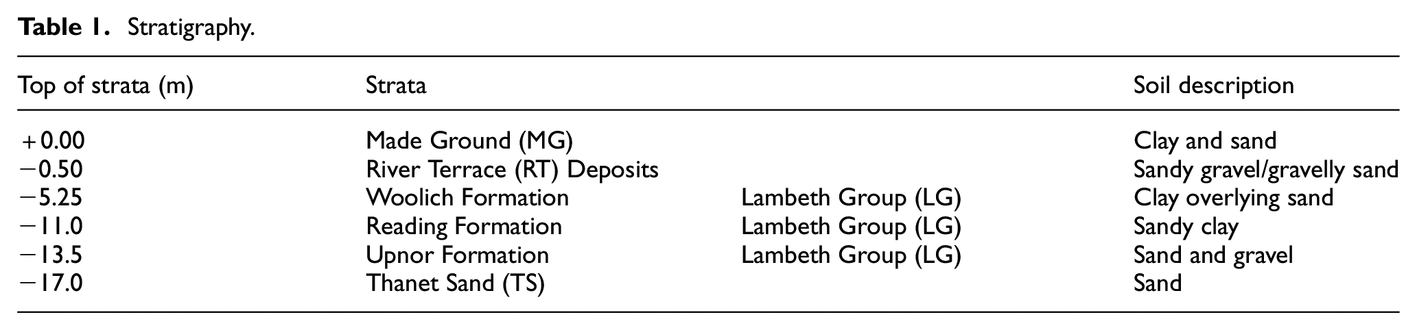
Stratigraphy.

Top of strata (m)	Strata		Soil description
+0.00	Made Ground (MG)		Clay and sand
−0.50	River Terrace (RT) Deposits		Sandy gravel/gravelly sand
−5.25	Woolich Formation	Lambeth Group (LG)	Clay overlying sand
−11.0	Reading Formation	Lambeth Group (LG)	Sandy clay
−13.5	Upnor Formation	Lambeth Group (LG)	Sand and gravel
−17.0	Thanet Sand (TS)		Sand

In this test, three engineered inclusions were attached to the cage at three different locations at three levels as shown in Figure 2. These locations were chosen to assess the ability of TIP to detect inclusions, internal and external to the cage, and demonstrate their effect on the pile curing temperature. Inclusion 1 consisted of sandbags with thickness of 70 mm. These bags were filled with Thanet Sand and attached externally to the reinforcement cage. Inclusion 2 is a water container filled with Thanet Sand. It was positioned centrally within the reinforcement cage with a diameter of 270 mm. Inclusion 3 was another water container with the same geometry as Inclusion 2, but it was positioned at the internal circumference of the cage, close to TIP-1.

Figure 2.

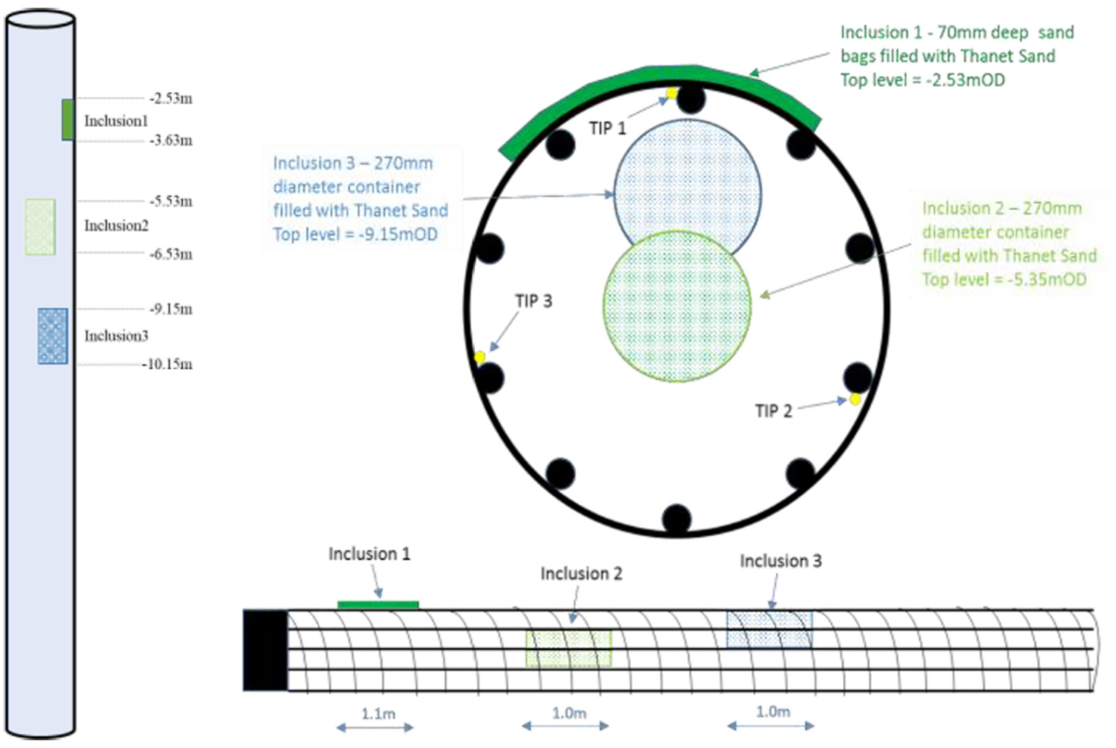
Engineered inclusions in the field test.

Data interpretation

If the CFA test pile was intact without any inclusions, the reinforcement cage is central and the surrounding soil is uniform, the measured temperature profiles should be uniform in shape and magnitude across the three different thermal cables. Temperature readings were recorded at 300 mm intervals along the pile length with each thermal cable providing a complete temperature profile at any specific time. The temperature measurement was initialised at 17:15 with a 15-min interval on 10 June 2015 and continued for 40 h after concrete placement. All the temperature data reported in this article represent the temperature change compared to the initial baseline temperature recorded at 17:15.

For a perfect cylindrical pile without any defect, the longitudinal temperature distribution is nearly constant within the same soil layer. The change of soil thermal properties between different strata affects the heat dissipation rate from concrete body to surrounding ground and leads to longitudinal temperature variation as shown in Figure 3. The soil with higher thermal conductivity allows faster heat transfer; thus, lower temperature would be recorded within the corresponding strata on the longitudinal temperature profile. Therefore, temperature measured in the River Terrace Deposits is supposed to be lower than that Lambeth Group and lower than Thanet Sand. Generally, a significant ‘roll-off’ would exist on both ends of the longitudinal temperature profile, as heat dissipates not only radially outwards but also vertically through the ends to the ambient environment (air) on the top or to the soil layer at the bottom.

Figure 3.

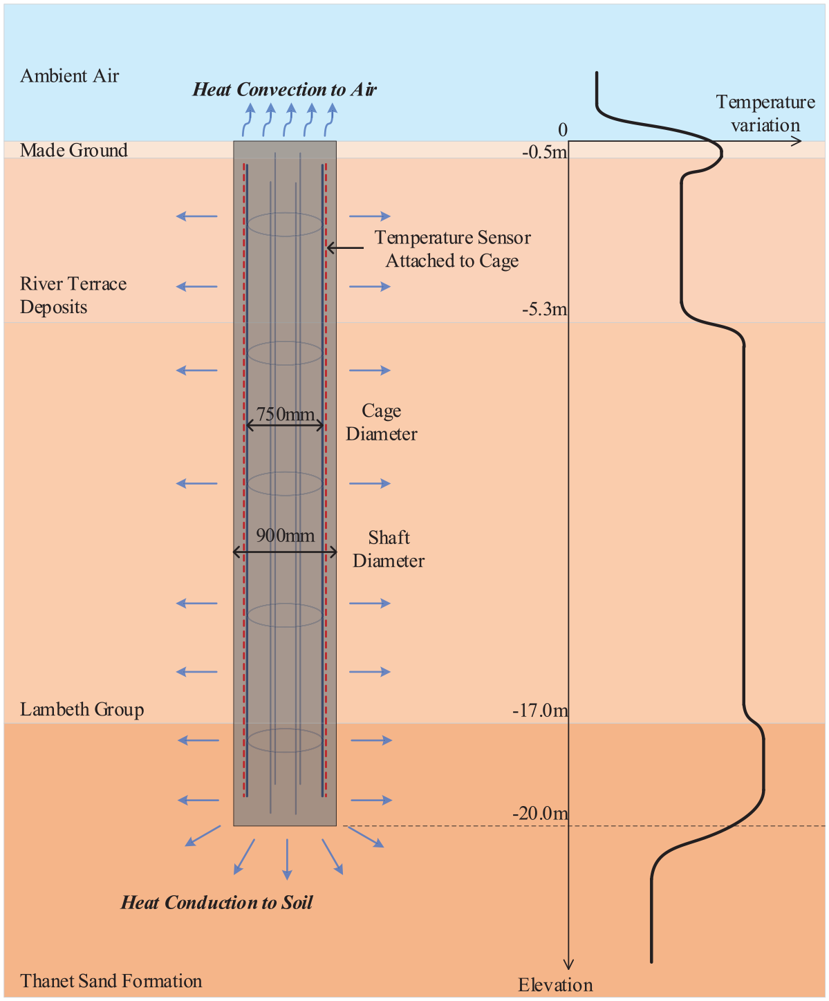
Longitudinal temperature variation profile for a perfect cylindrical pile without any defect.

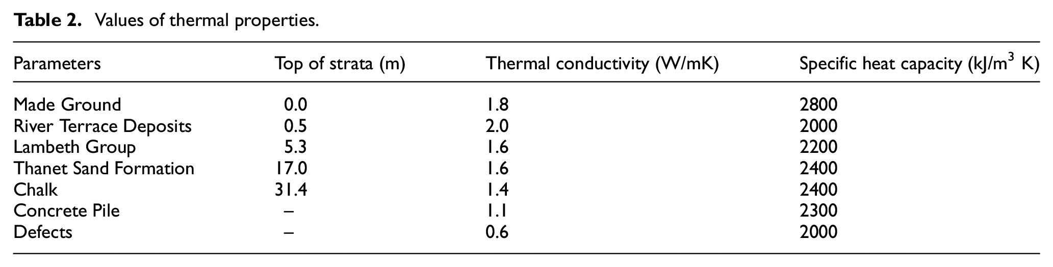
The measured longitudinal temperature variation profiles along the entire length of the test pile at four different stages are shown in Figure 4. The theoretical temperature development (assuming a perfect pile), obtained from a two-dimensional (2D) numerical analysis of a longitudinal cross-section of the pile (along the entire depth), has been superimposed on the figure. The 2D numerical analysis used different thermal properties that are appropriate for each soil layer as shown in Table 2 in this article. When comparing the field data and the numerical predictions in Figure 4, a number of points should be pointed out as follows:

• The 2D analysis adopted the thermal conductivity values shown in Table 2; for each soil layer, these are average values and it is acknowledged that these values may vary. For example, a range of values (1.51–2.37 Wm⁻¹ K⁻¹) has been reported in the literature for the Lambeth Group layer.^16–19

• The exact boundaries between the soil layers shown in Figure 4 are not certain. This is the authors’ best estimate based on the geotechnical investigation borehole.

• As the concrete hydration process is time-dependent, a number of publications^13,20,21 have suggested that the optimal times to distinguish regions of suspected anomalies in piles are the times corresponding to (1) the maximum rate of temperature rise and (2) the peak temperature. These correspond to 8 and 17 h, respectively, for the field test presented in this article. At 35 h, the heat of hydration reduces significantly, and the thermal conductivity of the soil surrounding the pile becomes more significant.

Figure 4.

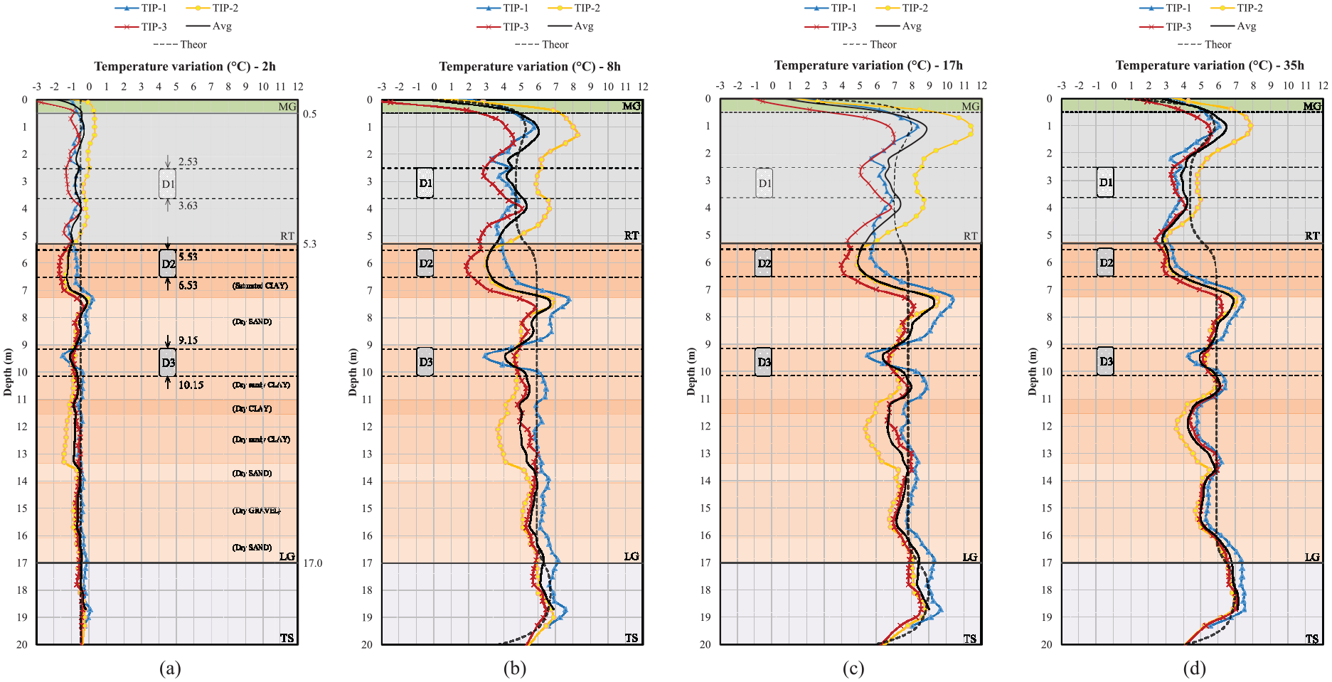
Longitudinal temperature variation profiles at (a) 2 h, (b) 8 h, (c) 17 h and (d) 35 h.

Table 2.

Values of thermal properties.

Parameters	Top of strata (m)	Thermal conductivity (W/mK)	Specific heat capacity (kJ/m3 K)
Made Ground	0.0	1.8	2800
River Terrace Deposits	0.5	2.0	2000
Lambeth Group	5.3	1.6	2200
Thanet Sand Formation	17.0	1.6	2400
Chalk	31.4	1.4	2400
Concrete Pile	–	1.1	2300
Defects	–	0.6	2000

At 2 h after the start of measurements, the temperature dropped by about 1°C–2°C along the four profiles as shown in Figure 4(a). This is due to the initial concrete temperature being higher than the ground temperature. The initial concrete curing was relatively slow as the temperature needed to reach an equilibrium before enough heat was generated from hydration to compensate that lost to the colder ground. Between 4 and 8 h, the whole pile began to heat up except for the top half metre, where concrete was exposed to ambient air at the night-time. At 17 h, the temperature variation profile of the whole pile reached the maximum value about 8°C–11°C. After that, temperature gradually decreased at a very slow rate. At 35 h, the average temperature variation of three cables fell inside a range of 3°C–7°C. The levels of engineered inclusions (D1, D2 and D3) and soil layers are also illustrated in Figure 4 where a theoretical temperature profile (in dashed grey) is plotted in each of the stages to assist in the determination of anomalies. The theoretical represents the theoretical temperature variations of an intact pile calculated numerically making assumptions for the thermal conductivities of the different soil layers.

Figure 5 demonstrates the change in temperature over the 40-h monitoring period for the three temperature cables on two cross-sections at 4.9 and 15.1 m depth. The observed temperature profiles showed a small drop in temperature over the first 2 h, followed by a steep increase for the subsequent 12 h. The maximum temperature changes at the depths shown were about 5°C–7°C and 6°C–8°C, respectively. As shown, the temperature profiles between different temperature cables were not uniform. The difference ranged between 1°C and 2°C.

Figure 5.

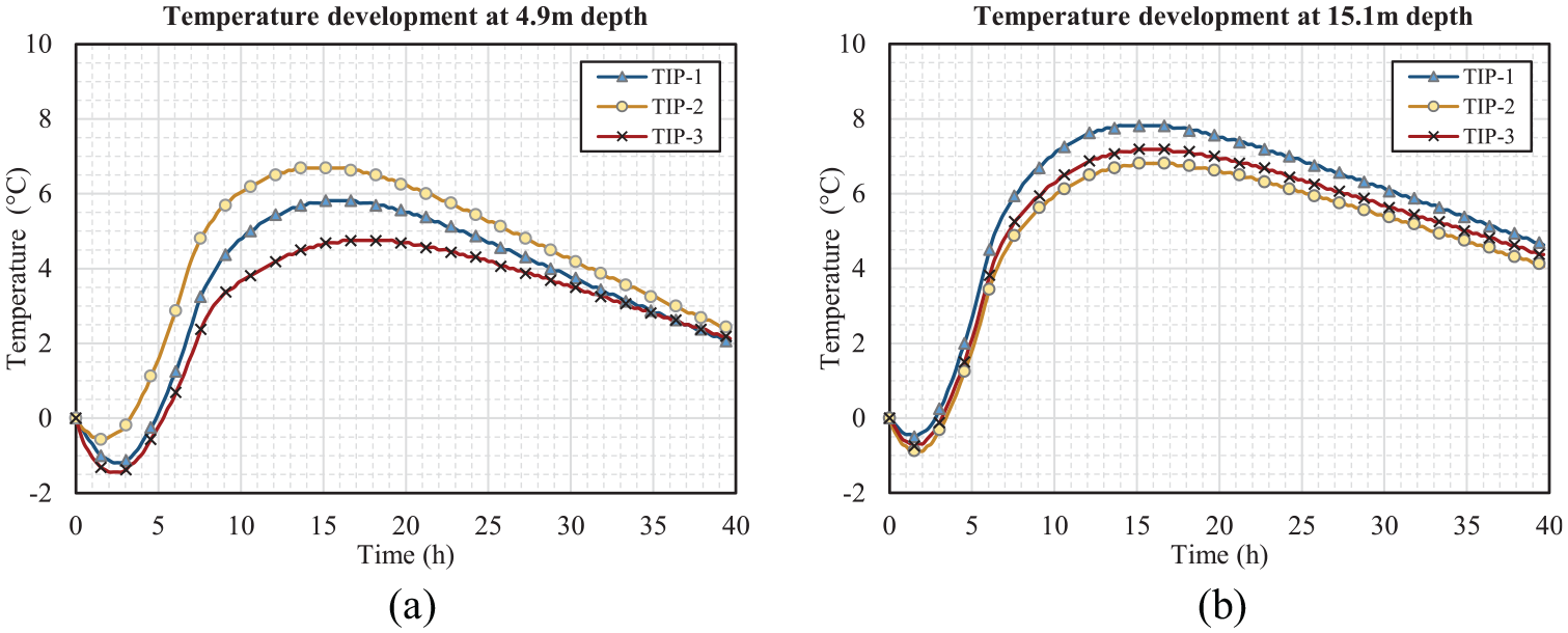
Thermal wire cable temperature development over time at two depths: (a) 4.9 m and (b) 15.1 m.

These temperature profiles discussed above are determined by a combination of factors, including the hydration heat produced by the concrete and the heat transfer rate between the pile and the surrounding soil. ¹⁰ If the measured temperature profile versus depth is consistent and each individual cable is also consistent, the pile is considered to be uniform in shape along the pile length, as shown in Figure 3. If not, it is assumed that some kind of defect existed in the pile as conceptually shown in Figure 6. In order to quantify the defects, a series of finite element (FE) analyses was then performed to back analyse the effects of these defects.

Figure 6.

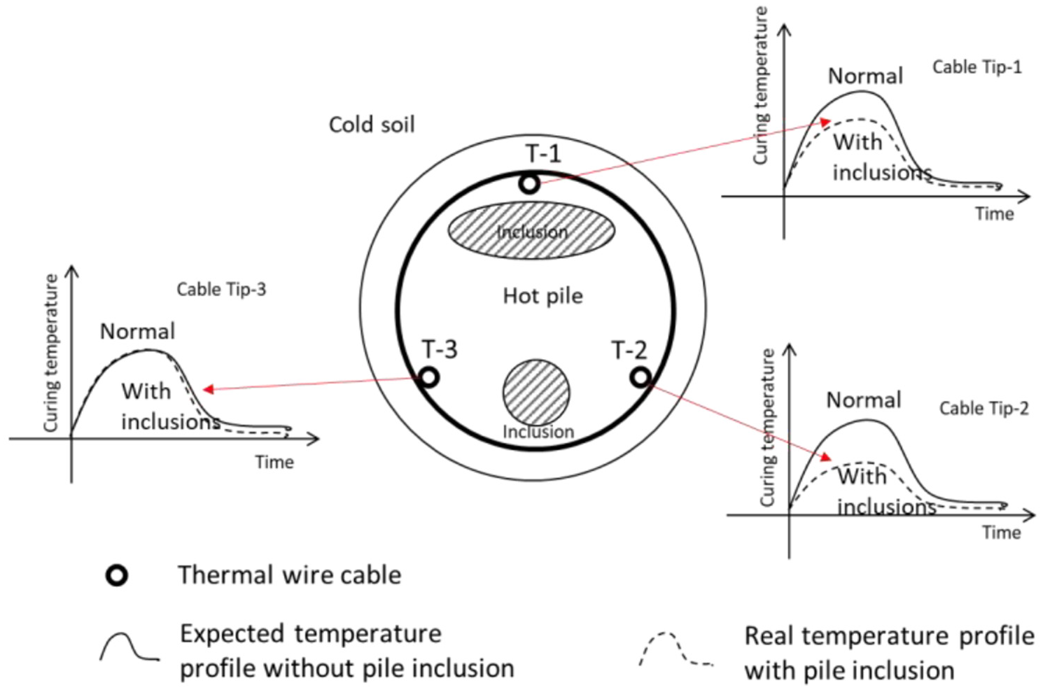
Conceptual relationship between temperature profile and pile integrity.

Numerical analysis

FE model

An FE model is developed to simulate the hydration and heat transfer process in this test. In this model, it is assumed that heat conduction is the major method of heat transfer. The fundamental law governing heat conduction is commonly referred to as the principle of conservation of energy

$$-\mathbf{tr}\nabla {\mathbf{q}}_{\mathbf{s}}+Q={\mathrm{c}}_{\mathrm{sw}}\stackrel{·}{\mathrm{T}}+{\mathrm{c}}_{\mathrm{sw}}(\mathbf{u}·\nabla )\mathrm{T}$$

(1)

where ${\mathbf{tr}\mathbf{\nabla }\mathbf{q}}_{\mathbf{s}}=\sum _{\mathrm{i}=1}^3/\partial \mathbf{x}$ , ${\mathbf{q}}_s$ denotes the heat flux, $\mathrm{n}$ denotes the direction vector normal to the integration surface, ${\mathrm{c}}_{\mathrm{sw}}$ is the specific heat capacity (unit: J/(m³ K)) considering the combination of soil and water content, $\mathbf{u}$ is the velocity vector of underground water flow, $\mathrm{T}$ is the temperature, $\stackrel{·}{\mathrm{T}}=\partial \mathrm{T}/\partial \mathrm{t}$ , and $Q$ contains the heat sources other than viscous heating.

The heat transfer interfaces use Fourier’s law of heat conduction, which states that the conductive heat flux, ${\mathbf{q}}_s$ , is proportional to the temperature gradient

$${\mathbf{q}}_{\mathbf{s}}=-{\mathrm{k}}_{\mathrm{ij}}\frac{\partial \mathrm{T}}{\partial {\mathrm{x}}_{\mathrm{j}}}$$

(2)

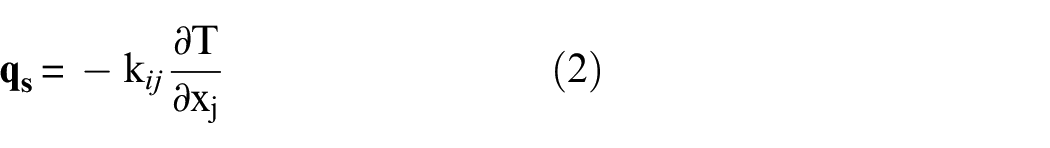
where $\mathrm{k}$ is the thermal conductivity.

Using these formulations, the FE model was developed to simulate the heat production and transfer of the test CFA pile during the curing stage. Due to the large pile length (20 m) compared to the cross-section of the pile (0.9 m), heat dissipates horizontally from concrete body to the surrounding soil with negligible vertical heat transfer along the length of the pile. Thus, the FE analysis of the test pile can be simplified as a 2D problem. At the tip and toe of the pile, heat can transfer vertically which violates the assumption of 2D heat transfer in the horizontal direction. However, the end effect is significant within 1-diameter depth near the pile top and bottom. ²⁰ Therefore, the FE analysis is conducted between the depths of 1 and 19 m.

A 2D mesh of this FE model at the depth of 9 m is shown in Figure 7, which includes soil, concrete and defects. The distance between pile centre and the mesh boundary is 5 m, which is far enough to deem any boundary effects insignificant. The FE analysis also confirmed that the hydration heat can only transport to a maximum distance of 3 m in the soil during the first 2 days after concrete casting. ¹⁰ The initial temperature of the soil was fixed at an assumed ground temperature of 13°C. The soil thermal properties vary for different soil strata as listed in Table 2. The values of these parameters are selected from a number of references.^{16–19,22–24} The defect elements in the mesh produce zero or only a small amount of heat corresponding to a soil inclusion or poor-quality concrete, respectively. The size, location and thermal conductivity of the defect are incorporated in the FE analysis according to the detailed information available from the site data. In this field case study, engineered defects were made of dry Thanet Sand; thus, defect thermal properties are selected accordingly. The concrete elements produce heat to simulate early age concrete heat generation according to the hydration model.

Figure 7.

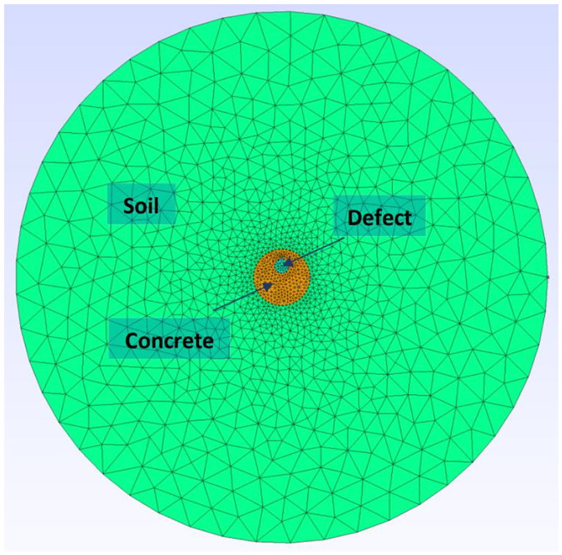
Finite element mesh for pile integrity testing.

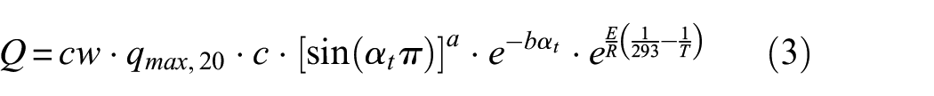
The accuracy of the hydration model will directly affect the FE temperature prediction and the anomaly detection capability. Many formulations have been developed over the years to quantify the hydration heat production; De-Schutter and Taerwe ²⁵ developed a classical hydration model based on their experiment results of isothermal and adiabatic cement calorimeter tests. They refined the model at a later stage through another series of tests and added the concrete strength relationship into the model. ²⁶ Schindler ²⁷ developed a hydration model based on concrete maturity where the concrete equivalent age and the Arrhenius rate theory were used for expressing the heat production rate. The model has then been optimised with some material parameters explicitly expressed through data regression from many cement experiments.^28,29 This model requires complicated hydration tests, and it is less practical in simulating site construction. Another model developed by Tomosawa and colleagues^30,31 studied the hydration process at the molecular level. It focuses more on determining chemical reaction coefficients as follows: the rates of formation and destruction of an initial impermeable layer, the activated chemical reaction process and the diffusion-controlled process, which is less accurate for modelling hydration heat.^32,33 In this study, the hydration model by De-Schutter and Taerwe ²⁵ was used. The model has explicit and relatively simple mathematical expressions. The heat production rate of concrete $Q(\mathrm{J}/\mathrm{gh})$ is expressed as a function of the actual temperature and the degree of hydration ²⁵

$$Q=\mathrm{cw}·q_{\max ,20}·c·{\left[\sin \left({\alpha }_t\pi \right)\right]}^a·e^{-b{\alpha }_t}·e^{\frac{E}{R}(\frac{1}{293}-\frac{1}{T})}$$

(3)

where $a$ , $b$ and $c$ are the hydration parameters dependent on material properties; ${\alpha }_t$ is the degree of hydration, defined as the proportion of amount of heat released at time $t$ to total heat of hydration; $q_{\max ,20}$ is the maximum heat generate rate at 20°C; $E$ is the apparent activation energy; $R$ is the universal gas constant; $T$ is the temperature of concrete $(\mathrm{K})$ ; and $\mathrm{cw}$ is the percentage of cementitious materials by weight, which is 16% in this case study.

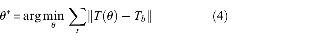
Model calibration by differential evolution

In the proposed approach, the field test temperature development is simulated with an FE model, which employs De-Schutter’s hydration model ²⁵ for predicting concrete curing heat. In order to demonstrate the generality of this method, it is necessary to utilise an effective calibration method to determine the corresponding hydration parameters for different concrete sources.

The concrete hydration heat is defined by a total of four parameters, grouped as a vector $\theta =\{a,b,c,E,q_{\mathrm{ma}{x}_{20}},Q_{\mathrm{total}}\}$ , the magnitudes of which can be determined by treating the model calibration as an optimisation problem, that is, to obtain a set of hydration parameters $({\theta }^{*})$ that minimise the difference between the hydration test data and the model simulation

$${\theta }^{*}=\arg \underset{\theta }{min}\sum _t\Vert T\left(\theta \right)-T_b\Vert$$

(4)

considering $T$ as a function of $\theta$ in the FE hydration model; and $T_b$ denotes the baseline temperature obtained from the hydration test. Ideally, a calorimeter hydration test is performed on site during concrete casting according to the ASTM standard. ³⁴ However, the method requires expensive equipment, complex testing procedures and extensive time; thus, it could be unsuitable for field applications. Wang et al. ³⁵ and Boulay et al.^36,37 have developed simple test apparatus and rapid experimental methods for monitoring the heat generation of concrete mixtures on site. Without a calorimeter test to measure concrete hydration heat for this project, an alternative approach is required to calibrate the hydration model. As no artificial defect was placed in the region 14–18 m and the temperature profile at this depth was relatively stable, the average temperature data of three cables along 14–18 m were selected as the baseline temperature $(T_b)$ for optimisation.

For efficient optimisation of the parameters, this study employs the heuristic algorithm known as differential evolution, which is conceptually similar to other evolutionary algorithms such as the genetic algorithm. Details of the differential evolution algorithm are described by Storn and Price ³⁸ and in recent engineering applications such as Leung et al. ³⁹ Essentially, a population of candidate solutions is first generated randomly in the optimisation process. The candidate solutions are vectors of the six variables (i.e. $\theta$ , known as trial vectors) in the optimisation problem. At each iteration (‘generation’), ‘mutant vectors’ are calculated by linear interpolation or extrapolation of trial vectors randomly selected from the population. A new generation of trial vectors is then formed by the ‘crossover’ process, whereby the components of the mutant vectors are mixed with those of the trial vectors in the previous generation. Fitness of trial vectors from the two generations (old and new) is evaluated and compared through a cost function, which evaluates the discrepancies between the FE model simulation and the temperature profiles obtained from the field test results in the depth range of 14–18 m. The fitness determines the survivability of the particular solution: the fitter solutions stay in the population, while the weaker ones are discarded. This procedure iterates until all solutions in the population converge to a single, global optimum solution, which is the optimised set of the six parameters $(\theta *·)$ in this study.

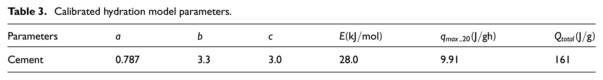
Applying the above procedure, the optimised hydration model parameters can be obtained as listed in Table 3. The optimised value of $Q_{\mathrm{total}}$ is slightly less than the value obtained from experimental data by De-Schutter; ²⁵ this is possibly due to the fact that half of the cementitious material has been replaced by ground granulated blast-furnace slag (GGBS) in this case study. All other parameters above are within close range to experimental hydration parameters reported in De-Schutter. ²⁵ Using the calibrated hydration parameters, the temperature prediction at 16 m depth can be obtained as shown in Figure 8. It shows a good agreement with the average field test average between 14 and 18 m depth.

Table 3.

Calibrated hydration model parameters.

Parameters	$a$	$b$	$c$	$E(\mathrm{kJ}/\mathrm{mol})$	$q_{\max \_20}(\mathrm{J}/\mathrm{gh})$	$Q_{\mathrm{total}}(\mathrm{J}/\mathrm{g})$
Cement	0.787	3.3	3.0	28.0	9.91	161

Figure 8.

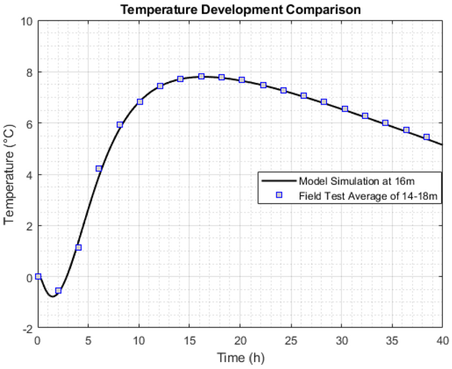
Model temperature (16 m) and field test temperature (14–18 m average) comparison.

Investigating the anomalies in the pile – the proposed interpretation approach

Preliminary direct observations

Having obtained an optimised set of parameters for the hydration model, the FE model was then used for back analysing the temperature development over the length of the pile (on the corresponding locations of the three thermal cables within the pile in the field). The aim of this back analysis is to assess the existence of the defects in the pile in order to validate the proposed interpretation method.

From direct observation of temperature profiles in Figure 4, several potential problematic zones are revealed. In 2–3 m depth, there was a sharp temperature reduction, which can be a concrete internal defect or a necking problem. In 5–7 m depth, temperature measurements significantly reduced at all three thermal cable locations. In 9–10 m depth, only TIP-1 exhibited a local temperature drop, while the other two cables were unaffected in this zone. This could result from a potential defect closer to the location of TIP-1 or a loss of cover thickness. The top and bottom temperature profiles tapered off consistently within one pile diameter (900 mm). The bottom of the shaft allowed heat dissipation longitudinally through the end and radially out to the sides; thus, the temperature reading was 3°C–5°C less than the average profile temperature in the lower 1-diameter length of the pile. Larger tapering was seen at the top. The top of the shaft was exposed to the air, and hence internal heat is dissipated much faster than the other boundaries. The open top did not reach the maximum temperature, and the readings rapidly tapered off by about 10°C. Therefore, the direct temperature profile observation revealed three major pile defects in 2–3 m, 5–7 m and 9–10 m zones. The FE analyses (described in later sections in detail) will focus on these three anomalous zones for investigation of the defect size and nature.

It is noteworthy to mention that the direct observation results agree with the location of the three artificial defects. The inclusions were designed at the levels of 2.53–3.63 m, 5.35–6.35 m and 9.15–10.15 m, respectively, which is within the abnormal readings’ zones observed in the temperature profiles. However, it is possible anomalies existed at 12 and 15 m depth. These were not taken further into consideration for the following two reasons:

• When there are changes in layers within the soil mass, the thermal boundary condition changes. Due to the different values of the thermal conductivities of the adjacent soil layers, sharp changes in temperature could be seen in the data. This is particularly relevant to the change in temperature observed at 12 m that coincides with the existence of a clay layer within a thick sandy clay layer.

• Taking into account the resolution of the temperature measurement system, changes that are consistently (as observed in Figure 4) within 1°C of the theoretical predictions were ignored. In case there was an anomaly, this small change in temperature implies only a small size defect that is unlikely to be of concern. This is relevant to the discrepancy at 15 m depth.

It is acknowledged that identifying the potential problematic zones, relying on direct observation only, could be subjective and a better method is required. Inclusion 1 was located in the granular saturated River Terrace Deposits. Inclusions 2 and 3 were located within the Lambeth Group, where soil was dewatered before construction. The thermal properties of the different soil strata are listed in Table 2. In the FE analyses, the soil properties play a critical role as the soil density and the amount of water affect the rate of heat dissipation from the concrete body to the surrounding ground.

Reinforcement cage alignment

In addition to the soil strata, the reinforcement cage alignment also affects the measured temperature profile. Pile reinforcement cages can be misaligned for various reasons including broken spacers, oversized excavation, bent cages and non-vertical or non-straight pile bores. The temperature in all three thermal cables at a certain level should be the same when the cage is centred. An off-centred cage will induce a temperature shift on the profiles, namely, cooler measurements from cables closer to shaft walls and warmer measurements from cables closer to the centre of the shaft. Therefore, when the reinforcement cage is not centred, a circular shaft can exhibit opposite temperature shifts from sensors on opposite sides of the cage. By comparing the temperature measurements from three cables on different sides of the cage, the cage offset direction can be determined. Therefore, the magnitude of cage eccentricity needs to be further assessed when using the FE model. Figure 9(a) is a schematic illustration of the location of the reinforcement cage and the three-dimensional (3D) view of the temperature distribution at 6 m depth. Comparing the thermal cable temperature measurements to the temperature distribution map from the FE model on the cross-section at 6 m depth (such as in Figure 9(b) the 2D view of the temperature distribution at 6 m depth), the amount of cage eccentricity can be evaluated.

Figure 9.

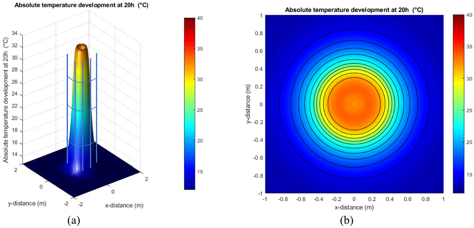
Temperature field and cage misalignment at 6 m depth cross-section: (a) the 3D view and (b) the 2D view.

From Figure 4, the temperature measurements on TIP-2 are constantly higher than TIP-1 and TIP-3 from 1 to 4.5 m depth throughout the 35 h of measurement duration. TIP-3 exhibits the lowest temperature, and TIP-1 is close to average temperature. This indicates that the cage is slightly offset to the northwest direction in this region. In the region of 4.5–8 m depth, TIP-1 shows a higher temperature on the profile and TIP-2 resembles average temperature, which indicates a cage offset to the southwest direction. From 8 to 12 m, the temperature measurements on TIP-2 and TIP-3 are similar. TIP-1 is closer to the pile centre and exhibits a higher temperature in the profile. Therefore, the cage is most likely offset southwards in this region. Getting an indication of the offset direction is important at this stage as this will be used in the detailed FE investigations that follow.

Detailed anomaly investigation using systematic FE simulations

The direct observation of temperature profiles gives a rough estimate of the potential anomaly locations within the pile length and also an estimate of the offset direction of the reinforcement cage if any. A detailed anomaly investigation process is then followed through a series of numerical modelling simulations as follows:

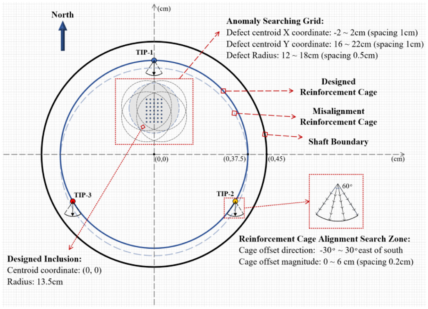
1. Taking a potential anomaly location into consideration, a numerical model is setup for a cross-section corresponding to each location within the pile depth at which a significant change in temperature has been observed from the field data. Looking at Figure 3(c), these depths correspond to 2.8, 6.1 and 9.4 m. Therefore, three 2D numerical models are setup for each location.

2. For each cross-section, the actual temperature readings from the three cables in the cross-section can give a rough indication of the location of an assumed circular anomaly within the cross-section. For example, if the three cables all reported a reduction in temperature at the same time as observed in depth 6.1 m, this suggests that the anomaly is centrally located within the section. If one cable shows a larger decrease compared to the other two as observed in depth 9.4 m (TIP-1 shows a larger decrease in temperature compared to the other two cables), this suggests the anomaly is internal (inside the reinforcement cage) and is closer to that cable and so on. The inference of defect location in this step is based on the assumption of a uniform shaft boundary. Necking and/or poor-quality concrete (among others) could cause similar temperature variations. It should be noted that while the TIP data could be fitted with a large number of equivalent interpretation models, the interpretation method proposed in this article focuses on the most common defects based on practical experience. The other point to raise here is that in reality, defects will be in 3D and hence a 3D analysis (outside the scope of this article) should provide better results. The effect of necking and poor-quality concrete is discussed in section ‘Cross-section at 2.8 m depth’.

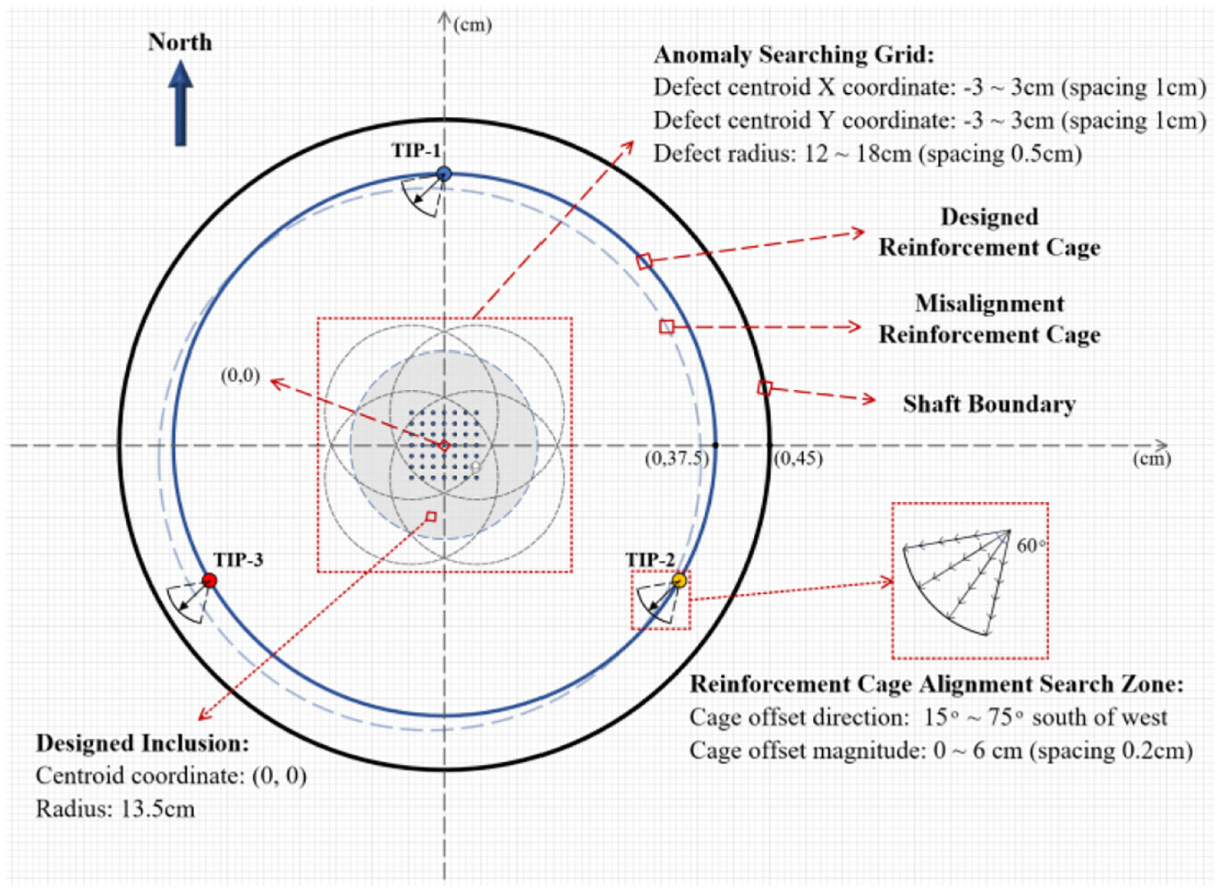
3. Based on this, for the section at 2.8 and 6.1 m depth, an assumed starting ‘search origin’ (0,0) is located at the centre of the cross-sections while for the section at 9.4 m, the starting ‘search origin’ is located at (0,19 cm) as shown in Figure 10. The above selection of the origin depends on the estimated defect locations from step (2). Note that it is also possible that the anomaly is external to the reinforcement cage; however, in this scenario (which will be investigated later for depth 2.8 m), the anomaly is expected to have a significant effect on the closest cable and little to no effect on the other two. This is the reason the ‘search origin’ at 2.8 m is not located close to the reinforcement cage even though the engineered Inclusion 1 is known to be in concrete cover region.

4. For each cross-section, a search grid zone is then setup around the search origin and a series of FE simulations is systematically conducted where a circular anomaly of changing radius is centred at each of the search grid zone points. For the cross-section at 6.1 m depth, the search grid (6 cm × 6 cm) had a total number of 49 search points. Numerical models were used to simulate circular anomalies centred at each of the 49 search points with the radius changing in size from 12 to 18 cm (adopting a step of 0.5 cm for each simulation) – a total of 637 2D FE simulations for the cross-section. The total number of simulations for the three cross-sections is 2469 (1377 FE simulations at 2.8 m depth and 455 FE simulations at 9.4 m depth).

5. After each simulation has been conducted (using the appropriate boundary conditions for the cross-section in consideration), the predicted temperatures at the location corresponding to TIP-1, TIP-2 and TIP-3 are compared to the actual field temperatures, and their cumulative temperature difference is set as the cost function that minimises the difference/error.

6. As discussed in the previous section, the reinforcement cage misalignment needs to be taken into account. As such, a search zone for the locations of TIP-1, TIP-2 and TIP-3 is then established within the numerical model in order to search for the minimum value of the cost function – this is to take the cage reinforcement offset into account at the end of each of the 2469 simulations. For each cross-section, this search zone assumes that the cage has shifted in and around the direction observed in section ‘Reinforcement cage alignment’.

7. At the end of FE simulations and cage misalignment searching, the anomaly configuration corresponding to the minimum cost function at each cross-section is selected and regarded as the detected anomaly.

Figure 10.

FE model defect configurations at 6.1 m cross-section.

Simulation results and discussion

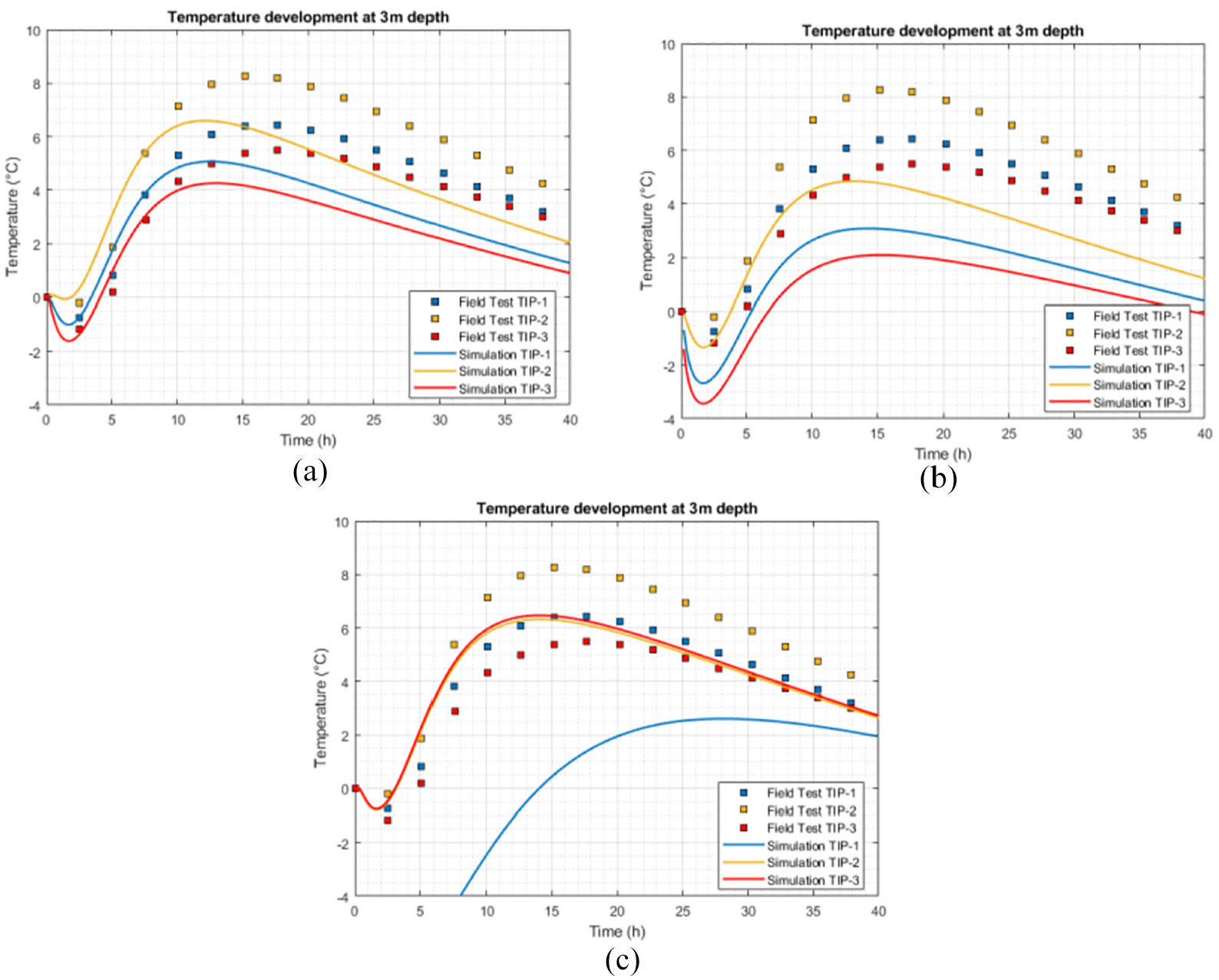
Cross-section at 6 1 m depth

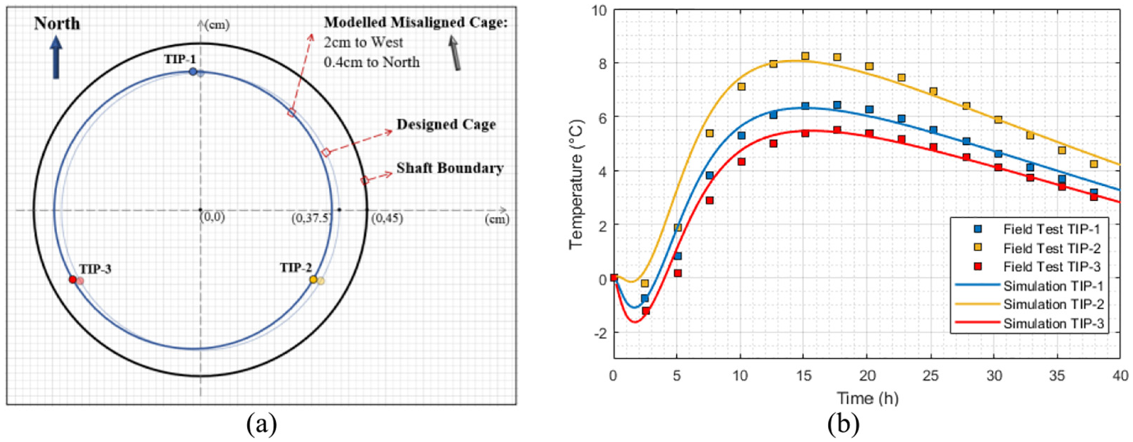
At 6.1-m depth level, all three cables show the same temperature reduction of 3°C–4°C at 17 h after concrete pouring compared to the adjacent temperature measurements. Thus, as discussed previously, the defect must have had an equal influence on the three cables, which indicates an existing inclusion around the centre of the pile cross-section. Following the procedure outlined in section ‘Detailed anomaly investigation using systematic FE simulations’, the anomaly configurations for minimising the cost function are shown in Figure 10. The results indicate the existence of an assumed circular anomaly centred at (−1 cm, 2 cm) with a radius of 16.5 cm accounting for 13% of the cross-sectional area and a cage eccentricity of 1 cm to west and 2 cm to south. Comparing the temperature measurements from three cables on different sides of the cage, as outlined in section ‘Reinforcement cage alignment’, the cage offset direction could be determined. The cage eccentricity direction and the magnitude in a Cartesian coordinate system are shown in Figure 11(a). A comparison between the predicted temperature development from the modelling and the field data at 6.1 m depth is demonstrated in Figure 11(b). The numerical results presented in the figure are the best predictions that could be generated among a total of 637 2D FE simulations for that section. Although the maximum temperature difference between the numerical predictions and the field data is small (within 15%) already minimised, there still exists some discrepancy. This may result from a number of reasons including the following:

1. A slight variation in the hydration process at this level and the lower half of the pile where the hydration model was optimised. The top and bottom parts of this pile were cast from two different concrete trucks at different times.

2. The variation of soil thermal properties in the Lambeth Group (different soil layers with different thermal properties) could also lead to such the discrepancy between the numerical and field data.

3. The analyses performed are 2D analyses; in reality, the anomalies are 3D. Hence, the model predictions will have to be viewed in that context.

Figure 11.

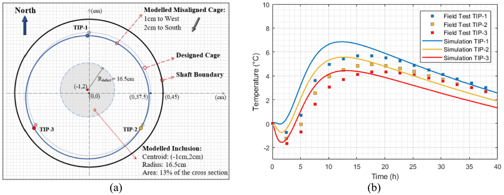
(a) Anomaly configuration and (b) predicted and actual temperature comparison at 6.1 m.

Cross-section at 9 4 m depth

At 9.4-m depth level, TIP-1 shows a steep drop of 4°C–5°C in the temperature profile at 17 h, and TIP-2 and 3 are relatively stable with minor temperature decrease, which indicates an existing inclusion near the TIP-1 cable in the shaft centre. Assuming a search grid zone centred at (0,19 cm) as shown in Figure 12 and following the procedure outlined in section ‘Detailed anomaly investigation using systematic FE simulations’, the FE simulation results predicted an inclusion centre at (−2 cm, 17 cm) with a size of 8% of the cross-section and a cage eccentricity of 4 cm to the south. The corresponding cage misalignment and temperature development are illustrated in Figure 13(a) and (b). Figure 13(a) follows the procedure outlined in section ‘Reinforcement cage alignment’ to evaluate the cage misalignment. Figure 13(b) presents the numerical predictions from 455 2D FE simulations at 9.4 m depth; the results agree well (within 9%) with the field data.

Figure 12.

FE model defect configurations at 9.4 m cross-section.

Figure 13.

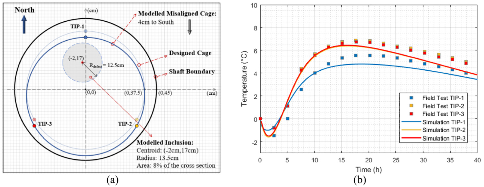
(a) Anomaly configuration and (b) predicted and actual temperature comparison at 9.4 m.

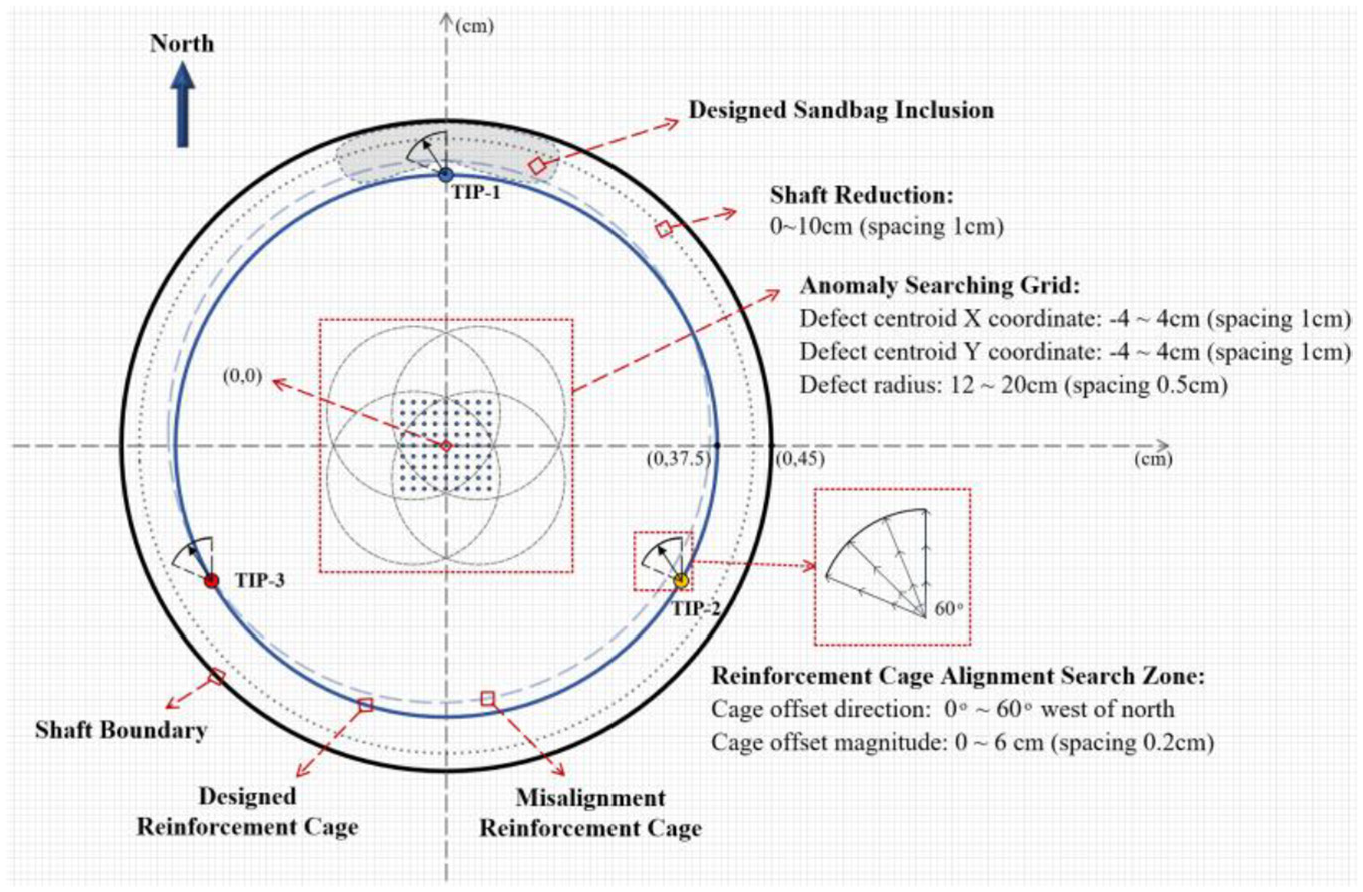
Cross-section at 2 8 m depth

At 2.8-m depth level, the sharp temperature reduction on all three TIP cables indicates a potential internal defect inclusion. It should be noted that this level is within the upper aquifer where heat dissipates more significantly from the concrete pile towards the soil. The high water content in the soil contributes to the temperature reduction at this level. The same procedure outlined in section ‘Detailed anomaly investigation using systematic FE simulations’ was implemented as shown in Figure 14. However, none of the numerical model results provided a credible match to the field data; the best temperature comparison is shown in Figure 15(a). In order to investigate such discrepancy further, a shaft diameter reduction (simulating necking) ranging between 0 and 10 cm was introduced into the FE simulations. The best matching simulation result for shaft necking, illustrated in Figure 15(b), still had a significant difference from the field test data. Based on the prior knowledge that the inclusion at this level is external to the cage (this could not be picked up from the field measurements as the three cables reported a reduction which is inconsistent with an external anomaly), an FE model was run with the defect assumed to be external to the reinforcement cage as shown in Figure 14, close to TIP-1 cable. Adjusting the defect size and location near TIP-1 cable, the simulation result still shows a significant difference from field data as presented in Figure 15(c). Therefore, the FE simulations did not give a clear indication of the existence of a defect or its nature at this level. Surprisingly, if no anomalies were included in the FE simulation (only cage misalignment taken into account), a good temperature development agreement can be found with a cage eccentricity of −2 cm to west and 0.4 cm to north as demonstrated in Figure 16(a) and (b). Upon further discussion with the site engineers, it was revealed that the inclusion (sandbags as shown in Figure 17) at the top broke during the concrete casting, and it is likely the sand has been mixed up with the concrete around the vicinity of the sandbag. This might explain why the FE simulations could detect a distinct anomaly as explained above.

Figure 14.

FE model defect configurations at 2.8 m cross-section.

Figure 15.

Predicted and actual temperature development at 2.8 m cross-section: (a) best result for a central defect, (b) best result for shaft necking and (c) best result for an inclusion in the concrete cover.

Figure 16.

(a) Anomaly configuration and (b) predicted and actual temperature comparison at 2.8 m.

Figure 17.

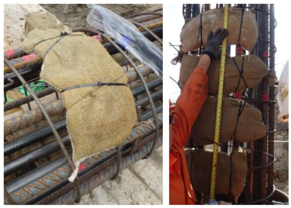
Site photos of sandbags.

Simulation result summary

Table 4 compares the actual defect sizes and locations with the FE model predictions. According to the results summarised in the table, the thermal integrity method gives an accurate prediction for Inclusions 2 and 3 in terms of size and location. The cross-sectional area for Inclusion 2 is slightly underestimated by 1% while the FE analysis over predicted Inclusion 3 by 4%. The predicted inclusion locations are marginally offset from the design by around 0.25 m in vertical depth and 3 cm on the cross-section. The small discrepancy between the actual and predicted locations may be due to construction documentation inaccuracies during installation, thermal cable installation process or variations of material thermal properties used in the FE models. The cross-section area (size) prediction for Inclusion 2 is more accurate than that for Inclusion 3, which may indicate that the thermal integrity interpretation approach is more sensitive to defects close to the temperature cables (Inclusion 2) and less sensitive to defects in the centre of the piles (Inclusion 3). Furthermore, the FE analyses did not detect Inclusion 1 – four sandbags were used to resemble a concrete cover defect attached externally to the reinforcement cage. The site resident engineer reported that these sandbags were actually broken during the reinforcement cage placement process. The sand spreads inside concrete body at this depth. As the volume of the sand was very small only constituting 3% of the pile cross-section area, the concrete quality appeared not to have been significantly affected.

Table 4.

Defect size and location by engineering design and thermal integrity testing detection.

Defect	Actual design				FE modelling
	Depth (m)	Area	Deff (cm)	Location (cm)	Depth (m)	Area	Deff (cm)	Location (cm)	Cage (cm)	Comment
Inclusion 1	3.08	3%	–	[0, 40]	2.8	–	–	–	[−2, 0.4]	Water
Inclusion 2	5.85	9%	27	[0, 0]	6.1	13%	33	[−1, 2]	[−1, −2]	–
Inclusion 3	9.65	9%	27	[0, 20]	9.4	8%	25	[−2, 17]	[0, −4]	–

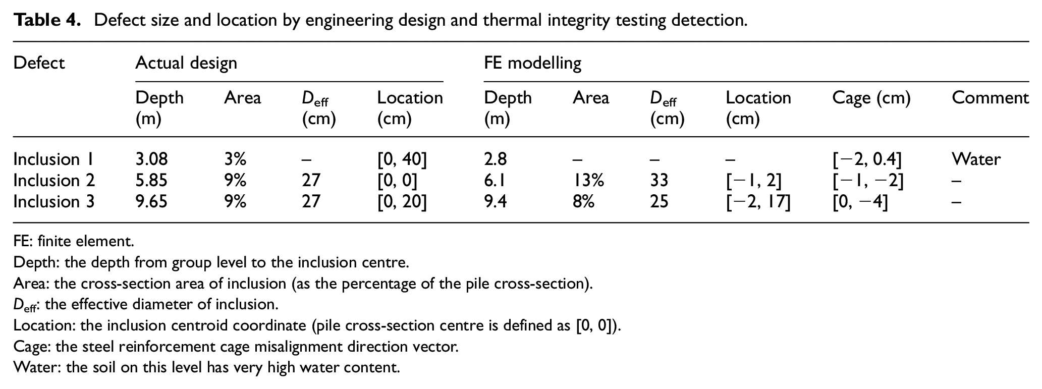
FE: finite element.

Depth: the depth from group level to the inclusion centre.

Area: the cross-section area of inclusion (as the percentage of the pile cross-section).

D_eff: the effective diameter of inclusion.

Location: the inclusion centroid coordinate (pile cross-section centre is defined as [0, 0]).

Cage: the steel reinforcement cage misalignment direction vector.

Water: the soil on this level has very high water content.

Proposed interpretation approach

Having conducted a detailed field case study for the thermal integrity testing, a framework is proposed to provide guideline of the data interpretation approach. This framework aims to facilitate the anomaly detection process for the cast in situ piles with higher accuracy. The basic elements of the proposed approach are shown in Figure 18. There are six processes shown in rectangular boxes, and their inputs and outputs are represented by elliptical shapes.

Figure 18.

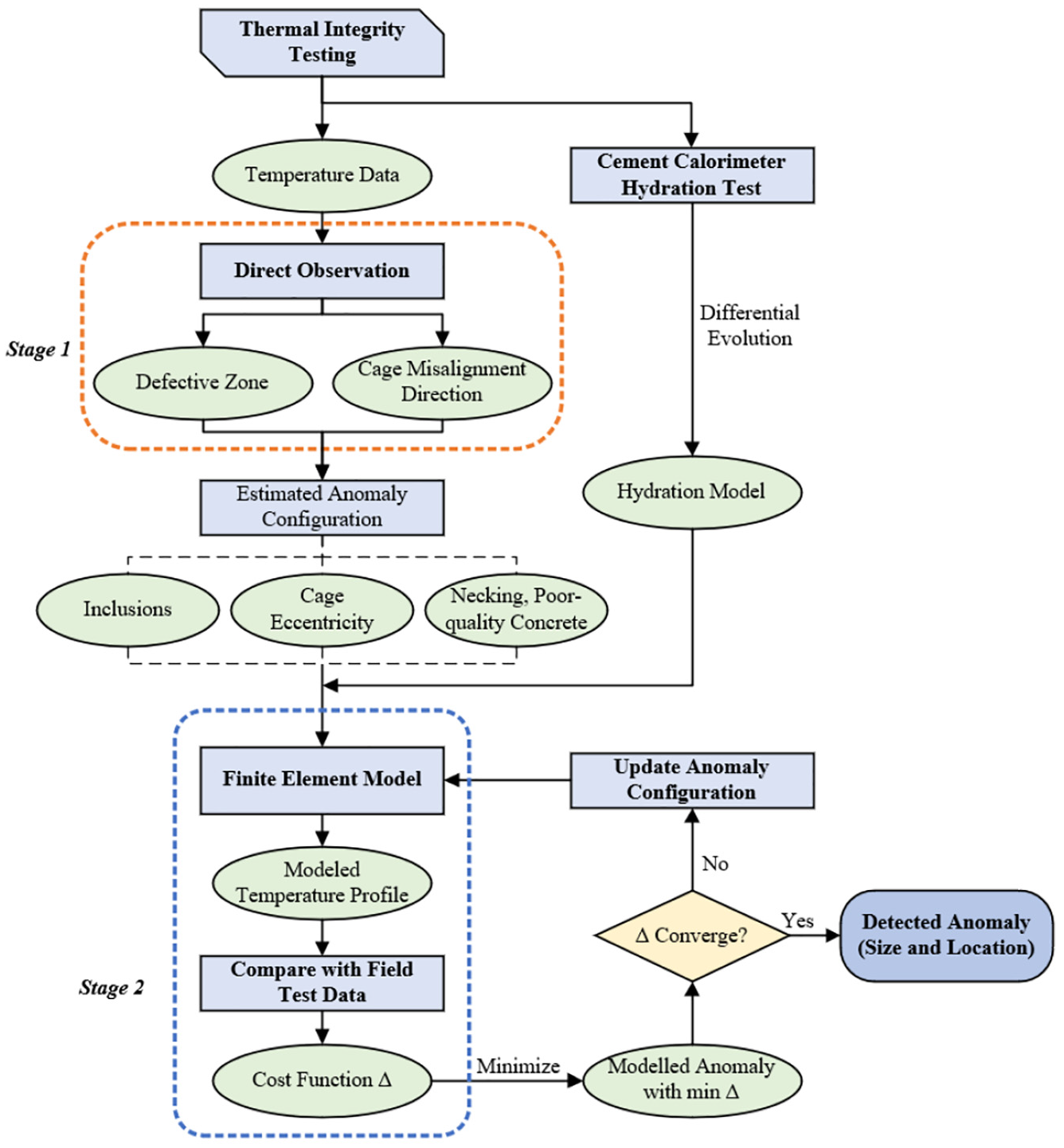
Proposed framework for thermal integrity testing data interpretation.

Thermal integrity testing is the first process. It can be achieved through deploying distributed or quasi-distributed temperature sensors on steel cages and recording temperature development for at least 48 h after concrete casting. In the meanwhile, a hydration test should be conducted in order to calibrate the cement hydration model. The obtained hydration model will be integrated into the FE model in the later stages. Upon obtaining temperature data from the first process, the data interpretation processes are divided into two stages. Stage one is the direct observation of the temperature profiles, which gives a rough estimate of the potential anomaly locations (defective zones with abnormal temperatures) and an estimate of the offset direction of the reinforcement cage, if any. The information retrieved from stage one is then used for setting up an anomaly search grid zone. The search grid can assist to configure different anomalies (with different sizes and at different locations within the search zone) in the FE model at stage two where a systematic defect searching process is conducted. This involves modelling temperature development of all the anomaly configurations and comparing the predicted temperature with the field data using an acceptable cost function (Δ). For an assumed anomaly (with an assumed size) at a specific location within the search zone, if the predicted temperature profile showed a significant difference from field data, a new anomaly configuration is input into the FE model. This is repeated, in a systematic manner, until a credible (within the acceptable cost function) anomaly configuration is obtained with size and location information. At this stage, using the numerical model, other credible interpretations should be checked (including necking, poor-quality concrete, etc.); eventually, the cost function could be used to appraise between all the different plausible interpretations. It should be pointed out that while in this article the anomalies are assumed to be circular in shape, in practice, the defects have a more complicated form and could comprise poor-quality concrete. This does not limit the modelling or the framework proposed below. Different shapes (with different sizes) could be assumed in the analyses and more shapes (with different sizes) could be added systematically within the same cross-section to minimise the cost function and get the best match possible.

Conclusion

TIP uses the temperature measurement of early age concrete to assess the integrity of underground structures including piles, diaphragm walls and so on. However, current data interpretation practice, and hence anomaly assessment through direct analysis of the temperature profiles, is currently subjective and relies heavily on limited experience given that TIP is relatively new. Due to this limited experience with TIP in the United Kingdom, a trial was conducted on an offline test CFA pile with known engineered inclusions (simulating anomalies in the pile) to evaluate the effectiveness of the method in (a) capturing detailed temperature data during the curing process as well as (b) propose a new interpretation method, based on the systematic use of FE numerical simulations, that addresses the shortcoming of translating the changes in temperature directly to changes in pile geometry currently used in practice.

The results show that TIP performed well in providing reliable and detailed temperature data for the assessment of pile integrity. Furthermore, the following conclusions are derived:

1. The thermal cables captured early thermal data very well and were capable of detecting all significant engineered inclusions in the trial pile. The advantage of using thermal cables is their capacity in providing a high spatial density of temperature data as well as the ease of installation during construction.

2. The new interpretation approach uses 2D FE simulations of the pile cross-sections at the locations where a significant departure from the theoretical temperature profile is observed. The FE simulations take into account an appropriate concrete hydration model as well as the thermal properties of the soil at the boundary of the cross-section. Introducing circular anomalies within the pile, whose size and location are initially informed by the actual temperature data from the field measurements, a systematic approach was then followed to obtain the best fit between the FE model predictions and the field data. The approach takes the cage reinforcement eccentricity, which could occur during cage installation in practice, into account.

3. In addition, an evolutionary optimisation technique was used to provide an inverse approach to characterise the concrete hydration model from the field data. This approach, using a differential evolution algorithm, can be used effectively to determine appropriate parameters for the heat hydration model which can be used in turn in the subsequent FE analyses.

4. The proposed new TIP interpretation approach was able to detect anomalies with less than 10% of the cross-sectional areas of the sections considered and could predict their sizes and locations with high accuracy. The method is more sensitive to anomalies that are close to the temperature measurement cables and less sensitive to anomalies at the centre of the cross-section.

5. The proposed framework of data interpretation in this article has its limitations. The numerical modelling presented was based on a uniform shaft assumption; this may not be the case in reality and hence the interpretation needs to be carried out in conjunction with available pile records. In addition, complex shapes of anomalies are not currently incorporated in the 2D modelling, and this could be improved. Moreover, identifying the potential problematic zones (relying on direct observation only) and appraising the plausible defect scenarios at the end of the numerical modelling could both be subjective and hence requiring good experience and sound engineering judgement.

6. The proposed approach, which could be developed further using 3D FE simulations and employing genetic algorithms on the FE predictions, could address some of the major shortcomings of the current interpretation method used in practice.

7. More laboratory trials and field trials are needed to further validate the proposed framework for thermal integrity testing data interpretation. This can help to improve the method and further increase the accuracy of anomaly detection.