
Abstract
Acoustic emission (AE) signals caused by valve leakage exhibit obvious nonlinearity and nonstationarity characteristics. Due to the limitations of traditional valve leakage diagnosis methods, it is difficult to distinguish between internal and external valve leakage failures effectively. Recognizing this challenge, a comprehensive valve leakage diagnosis method based on a multichannel fusion convolutional neural network (MCFCNN) is proposed. First, AE signals are converted from one-dimensional time-domain signals to two-dimensional time–frequency images by the time–frequency analysis method. Then, the time–frequency images are used as model inputs, and MCFCNN fuses the features of time–frequency images from two different position. Hence, a new comprehensive diagnosis method for the bi-sensor fusion contains the time–frequency information, modal information, and position information of valve leakage is proposed. Subsequently, the effectiveness of the proposed method was verified through valve leakage simulation experiments. Furthermore, in order to study the impact of modal information on identifying internal and external valve leakage faults, the fault prediction performance of MCFCNN was compared and analyzed using short-time Fourier transform (STFT) and time-reassigned synchrosqueezing transform (TSST). Finally, according to the needs of engineering practice, the impact of sampling length on different methods is studied. The results show that compared to STFT–MCFCNN, TSST–MCFCNN required a shorter sampling length with the same diagnostic accuracy, which means that the method proposed in this study can achieve faster response time for ball valve leakage under conventional leakage flow rates.
Introduction
Valves are control devices in fluid pipelines that have long-term exposure to high temperature, high pressure, and strong corrosion due to harsh environments. With the growth of service time, its control performance gradually declines. Hence, internal or external leakage failures often occur, thus leading to control failures, frequent accidents, and other production problems. Currently, the internal and external leakage monitoring of valves can be achieved by a single detection technique. However, no effective method has been formulated to achieve the simultaneous monitoring of the internal and external leakage of valves. The risks of the internal and external leakage of valves exist simultaneously. Therefore, the development of a comprehensive diagnostic method that can monitor these leakages is of great theoretical value and practical significance to maintain the safety of pipeline networks and avoid wasting resources.
For structural health monitoring, scholars have proposed various diagnostic techniques and methods, including manual inspection method, vibration analysis method, 1 pressure drop detection method, ultrasonic monitoring method,2,3 infrared thermal imaging technique, 4 and acoustic emission (AE) technique. 5 AE has become a research hotspot due to its sensitivity to leaked information. For instance, Ye et al. 6 analyzed the AE mechanism and characteristics of internal valve leakage and determined the theoretical relationship between the standard deviation of valve leakage AE signal and leakage rate. This correlation laid the foundation for the online detection of valve leakage under different working conditions. Furthermore, Li et al. 7 conducted an experimental study on acoustic emission-based leak detection of faulty water delivery systems and verified that the propagation distance and leak rate have little effect on the classification features from the perspective of pattern recognition.
Deep learning (DL) methods can effectively solve the problem of extracting and classifying leak-related information, among which convolutional neural networks (CNNs) shine with their powerful nonlinear mapping capabilities. CNNs can extract leak-related discriminative information from acoustic signals and use it for leak status classification.8–10 In one research, Guo et al. 11 demonstrated that CNNs exhibited better learning ability than back propagation neural networks (BPNNs), radial basis function neural networks, and support vector regression in predicting hydraulic cylinder leaks. Time–frequency analysis (TFA) techniques can reveal the dynamic properties of nonstationary signals, which can greatly improve the feature learning capability and pattern recognition accuracy of DL algorithms. 12 Wang et al. 13 processed the vibration signals into wavelet transform (WT) images and used them as input to a CNN, thus achieving good classification results. Moreover, Yuan et al. 14 first converted the time series of vibration signals into time–frequency images by Hilbert–Huang transform (HHT) and then used CNNs to learn fault features from the images to achieve the rolling bearing fault category and classification of fault severity. Kumar et al. 15 used wavelet synchrosqueezed transform to preprocess the data and apply them to a CNN to identify defects, which has a significant diagnostic accuracy advantage over traditional methods.
AE sensors are often arranged on the pipe wall to pick up the AE signal of the leakage. However, the AE signal generated by the external leakage of the valve is easier to pick up because the internal leakage of the valve occurs inside the pipe. In a complex environment, the measured AE signal caused by internal leakage generally contains strong background noise. AE signals caused by leakage exhibit obvious nonlinearity and nonstationarity characteristics.16,17 Hence, the analysis of the signal measured by a single sensor has difficulty obtaining comprehensive fault characteristics, thus affecting the accuracy of fault identification. As a solution, the multisensor information fusion method offers the possibility of extracting fault characteristics comprehensively and accurately. Gong et al. 18 proposed an improved CNN–SVM model to improve the accuracy of rolling bearing fault monitoring by using data from multiple sensors. Liu et al. 19 designed a multichannel fusion convolutional neural network (MCFCNN) and two one-dimensional CNNs to build an integrated model; moreover, they proposed an ensemble CNN bearing fault diagnosis model based on multisensor data to improve the information loss problem in the fault diagnosis process. In another study, Xia et al. 20 fused raw vibration signals from multiple sensors at different positions as CNN inputs, taking into account temporal and position information from multiple sensors, to improve the accuracy and reliability of fault diagnosis.
The AE signal is caused by valve leakage propagating along multiple paths, including the gas inside the tube and the tube wall; furthermore, the AE signals in different transmission paths have different modal distributions and different dispersion behaviors. 21 The direction of leakage differs between the internal and external leakage of a valve. Therefore, a difference exists between the modal information in the AE signal of the internal and external leakage. This difference is complex and cannot be effectively distinguished using conventional methods. Traditional filtering and spectral analysis techniques have difficulty distinguishing between different modal components in time–frequency domain mixed signals. Nevertheless, the TFA method gives the distribution of the time-varying energy flow density for each frequency component of the time-domain signal and can analyze multimodal mixed signals. 22 Unfortunately, common TFA methods, such as the short-time Fourier transform (STFT), WT, and HHT, have difficulty characterizing modal information clearly until the advent of the simultaneous compression transform (SST), which solved this problem. The SST is capable of producing the time–frequency representation with high-energy aggregation for nonsmooth signals. However, most conventional simultaneous compression techniques implicitly assume that the signals analyzed exhibit slow time-varying properties, whereas leakage generates AE signals that can occur over very short durations with wide frequency bands. Therefore, the slow time-varying model is no longer valid in this case. Recently, for strongly time-varying signals, He et al. 23 proposed a TFA method for time–frequency aggregation, time-reassigned synchrosqueezing transform (TSST), which has good results for TFA of pulse-like signals.
In summary, the main challenges in diagnosing valve leaks are summarized below.
The diversity of valve leakage fault types and the complexity of the environment in which they are located cause difficulty in using a common mathematical model or a single characteristic parameter to identify fault types.
The two types of faults, internal valve leakage and external valve leakage, show strong similarities in the time and frequency domains. An accurate classification of these two faults is difficult to achieve using conventional methods based on the time or frequency domains.
AE sensors are insensitive to internal leakage, thus creating difficulty in analyzing the signal measured by a single sensor to obtain a comprehensive fault signature and affecting the accuracy of fault identification.
Although the internal valve leakage and external leakage signals have modal differences, the form of this difference is complex and difficult to distinguish. In addition, the conventional TFA methods cannot obtain clear modal information of the leakage AE signal.
Focusing on engineering practice, this study proposes a comprehensive diagnosis method for valve leakage based on MCFCNN using a combination of offline training (source domain) and online monitoring (target domain). The time–frequency images containing time–frequency information and modal information are obtained using the time–frequency aggregation method, and the time–frequency images from two positions are fused with features by MCFCNN. A new comprehensive diagnosis method for the bi-sensor fusion contains the time–frequency information, modal information, and position information of valve leakage was proposed. In the offline training process, the time–frequency representation method of time–frequency aggregation is used to obtain the time–frequency images of no leakage, internal valve leakage, and external valve leakage under various operating conditions in the source domain. Then, train the MCFCNN network and save it. Finally, it imports the saved model parameters in the source domain into the comprehensive valve leakage diagnosis model in the target domain to achieve online monitoring, which solves the drawback that the traditional valve fault diagnosis cannot monitor both internal and external valve leakage faults under complex operating conditions. After experimental verification, the comprehensive MCFCNN-based diagnosis model for valve leakage has higher prediction accuracy than the traditional neural network model. The method described in this study still shows high prediction accuracy after reducing the sampling length of the input samples. Hence, the method proposed in this study can achieve faster response times in engineering practice at the same recognition accuracy.
The rest of the article is organized as follows: Section “Method” shows the details of the proposed detection method. Experimental results and discussion are given in Section “Experiment.” Finally, conclusions are given in Section “Conclusion.”
Method
Time–frequency aggregation method for AE signals
The AE signal caused by valve leakage propagates along multiple paths, including the gas inside the tube and the tube wall, the AE signals in different transmission paths have different modal distributions and different dispersion behavior. 21
In this study, the leakage process of the valve is simulated numerically. Collected the AE signals during the leakage process along the pipeline. Composed a position–time matrix using the collected signals at different positions as row vectors and transformed it into a frequency–wavenumber domain matrix through a 2D Fourier transform. 24 Finally, the obtained dispersion curves are matched with the known dispersion curves 25 to obtain the results shown in Figure 1. The internal and external leakage of the valve excites the bending mode (F mode) and the longitudinal mode (L mode). The bending mode component is slightly larger than the longitudinal mode. However, when the valve leaks externally, the proportion of the longitudinal mode (L mode) is significantly higher, thus causing a difference in the modal information between the internal and external leakage. This difference takes a complex form and cannot be effectively distinguished using conventional methods.
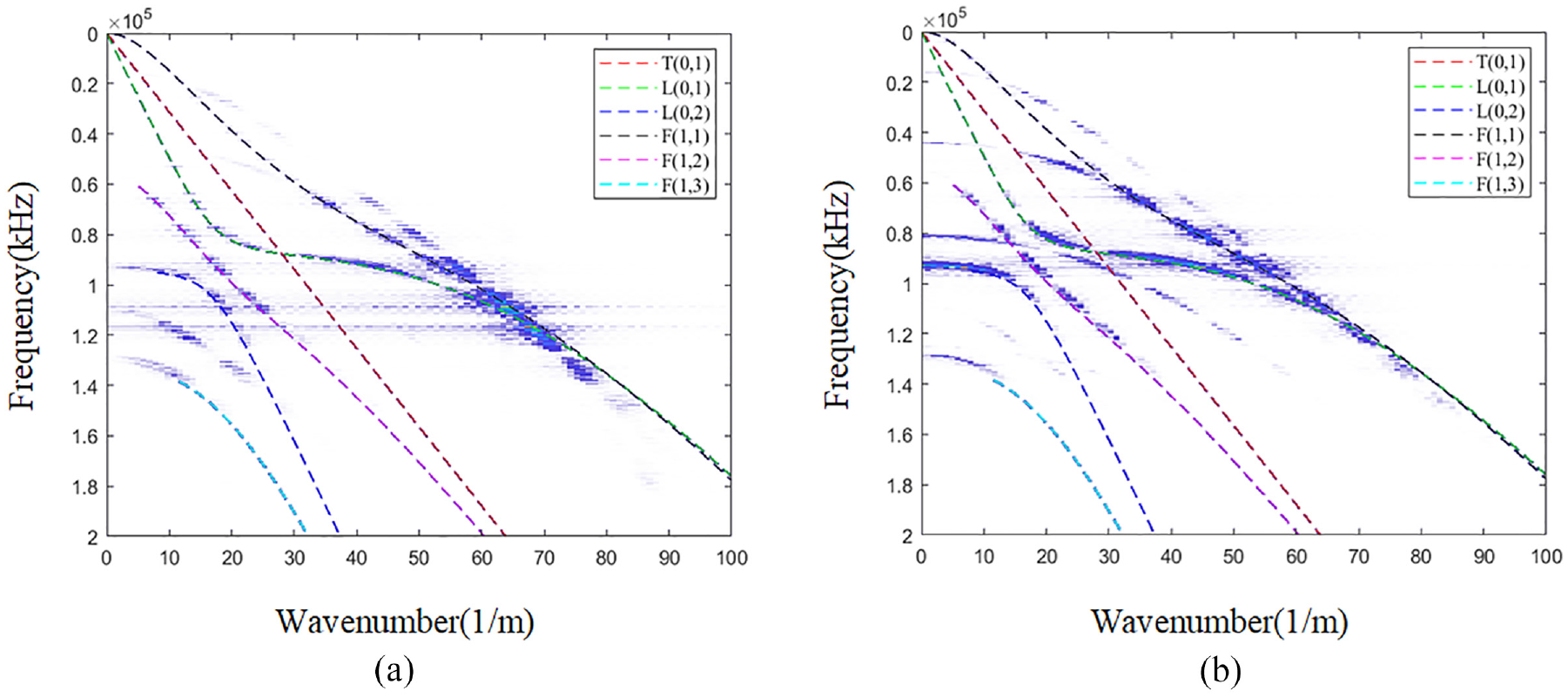
Difference between (a) internal and (b) external leakage modes of valves.
Compared with the original time-domain signal, the TFA results can show the time–frequency domain information of the signal, whereas the time–frequency energy aggregation method can characterize the modal information of the AE signal. Therefore, the time–frequency representation with high-energy aggregation contains the time–frequency domain and the modal domain information, which helps to improve the feature learning ability and pattern recognition accuracy of the DL algorithm.
The leaked excited ultrasound guided wave signal is expressed in Equation (1) 23 as
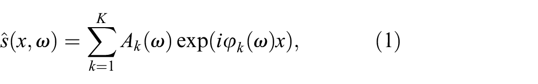
where
Performing the STFT using Equation (2):
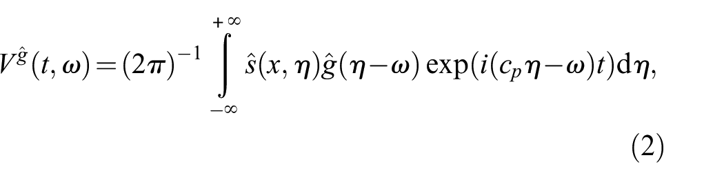
where
The computation of the classical group delay estimates for signals is expressed as Equation (3):
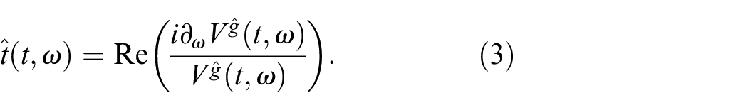
The time–frequency coefficients at
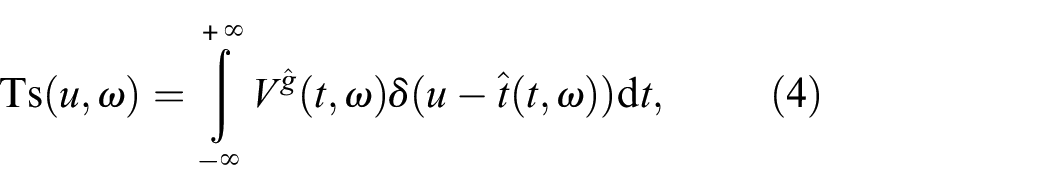
where
Multichannel fusion convolutional neural network
The CNN can perform feature depth extraction and recognition on time–frequency images. The training process of the CNN classification model consists of forward propagation and backward propagation. The forward propagation goes through the convolution layer and the pooling layer for the feature extraction and dimensionality reduction of the input time–frequency image. The classification is performed in the fully connected layer.
The signal measured by a single sensor has difficulty characterizing the fault comprehensively, thus affecting the accuracy of fault identification and failing to capture the overall changes in the leakage process accurately. Recent research has shown that the MCFCNN is effective in multifeature classification. 26 The MCFCNN has multiple channels in the input layer to process multichannel data separately. The main idea is to enhance the classification effect by extracting the coupled features of different sensors through multiple independent channels. This principle is shown in Figure 2. Given that the multichannel inputs are trained simultaneously under the same learning framework and the parameters of the different channels can be jointly optimized during training, the MCFCNN has better performance than a single-channel CNN.
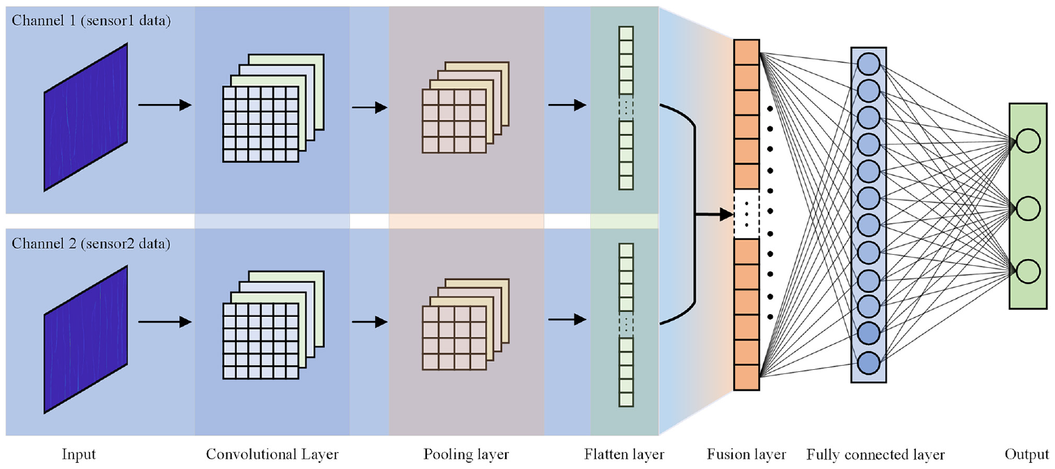
MCF–CNN schematic.
Assuming that layer l is the convolutional layer and layer l − 1 is the pooling or input layer, we obtain Equation (5):
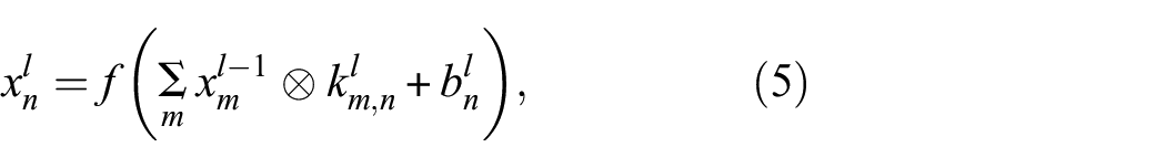
where
The pooling layer is usually designed to follow the convolutional layer to control overfitting effectively by gathering valid information from the feature maps extracted from the convolutional layer. Meanwhile, the process increases the robustness of the network and reduces the input size and network parameters of the next layer. In this study, a max-pooling layer is used to perform the pooling operation.
Comprehensive diagnosis method of valve leakage
This study addresses the problem that the traditional valve leakage diagnosis method has a low accuracy rate and cannot diagnose both internal and external valve leakage faults. It proposes a new comprehensive diagnosis method for valve leakage using the time–frequency image of time–frequency aggregation as the model input. Moreover, this study introduces time–frequency information, modal information, and position information to achieve the simultaneous monitoring of internal and external valve leakage faults and improve the accuracy of valve leakage fault identification further.
Data preprocessing
The experimentally measured AE signals for valve leakage are used as the source domain. The time–frequency representation of the AE signal is performed by the time–frequency aggregation method. In addition, the time–frequency signal of the valve leakage measured by the two AE sensors in the source domain (offline data) is sliced and converted to the time–frequency domain. Then, the labeled time–frequency image is used to train the MCFCNN-based comprehensive diagnosis model for valve leakage.
Time-reassigned synchrosqueezing transform–multichannel fusion convolutional neural network
To meet the needs of the online integrated monitoring of valve leakage, this study develops a two-channel MCFCNN based on time–frequency aggregation. TSST–MCFCNN converts AE signals collected by different sensors into time–frequency images via TSST. Then, it inputs the time–frequency images into different channels to achieve bi-sensor information fusion. The number of convolutional layers, kernel size, and activation function are the same for both branches of MCFCNN. The input image is first extracted from the depth features through three times of “convolution-normalization-activation-pooling.” Then, group normalization 27 is used to improve the training and convergence speed. Next, ReLU 28 is used as the activation function. Furthermore, the pooling method is max-pooling, and the extracted features are flattened by using the flatten layer at the end of the branch to transform the data into a 1D feature vector. The feature vectors from the two sensors are connected at the fusion layer. After the fusion layer, a fully connected layer is used to classify faults in the input signal with the number of neurons corresponding to the class of the classification task. The model described in this study has three classification results, namely, internal valve leakage, external valve leakage, and no leakage. The SoftMax function is used to convert the vectors of the fully connected layer into the form of a probability distribution. The TSST–MCFCNN model is shown in Figure 3.
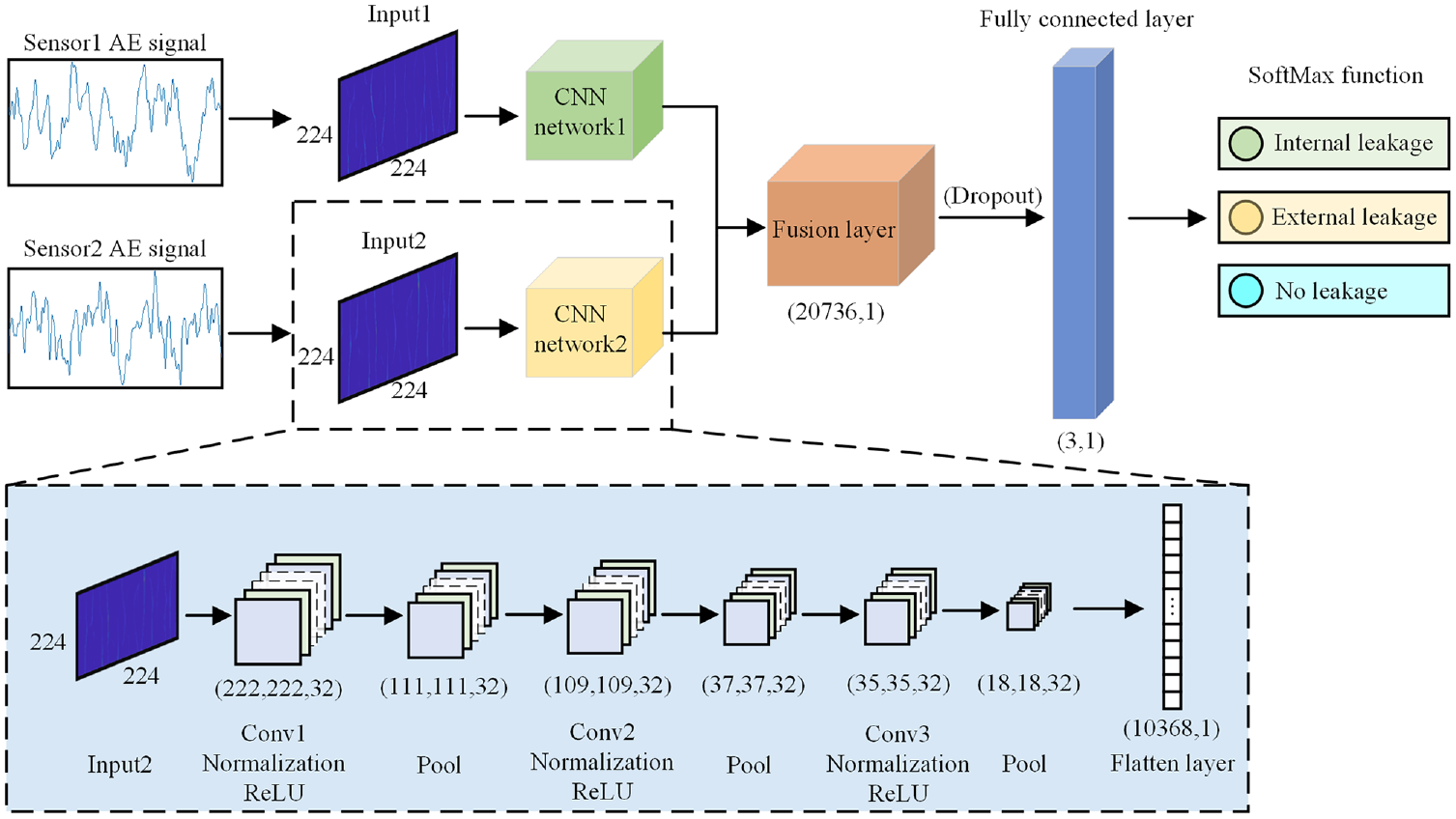
TSST–MCFCNN model structure.
Offline training
The generalization performance of the comprehensive valve leakage diagnosis model is closely related to the diversity of the source domain dataset. 29 Therefore, during the offline training process, internal leakage, external leakage, and no-leakage AE signals from valves under a variety of operating conditions are collected using two AE sensors, which include common internal and external leakage flows and no-leakage noise, and noise mainly includes artificial noise and laboratory environmental noise. The artificial noise is used to simulate the noise that may be generated in the actual working environment, including metal impact noise and plastic impact noise. The laboratory environmental noise is used to simulate normal environmental noise and industrial equipment operating noise, such as pumps. The collected AE signals are processed into time–frequency domain images as source domain data by TSST. The processed source domain data are placed into the built TSST–MCFCNN model for training. Different channels of data are trained in parallel. Then, the extracted feature maps are flattened using the flatten layer at the end of the channel, merged into a single channel of data in the fusion layer, and back-propagated by the SoftMax function error to optimize the model. The source domain model parameters are saved when the model reaches convergence.
Online monitoring
The AE signals collected by the online monitoring system are defined as the target domain, in which two AE sensors are used to collect the AE signals and convert the collected signals into TSST time–frequency domain images as the data to be diagnosed. The parameters of the offline training model are placed into the target domain TSST–MCFCNN. When the data to be diagnosed are input into the network model, fault classification is performed by TSST–MCFCNN. Then, the final fault diagnosis results are output. The schematic diagram of the model is shown in Figure 4.
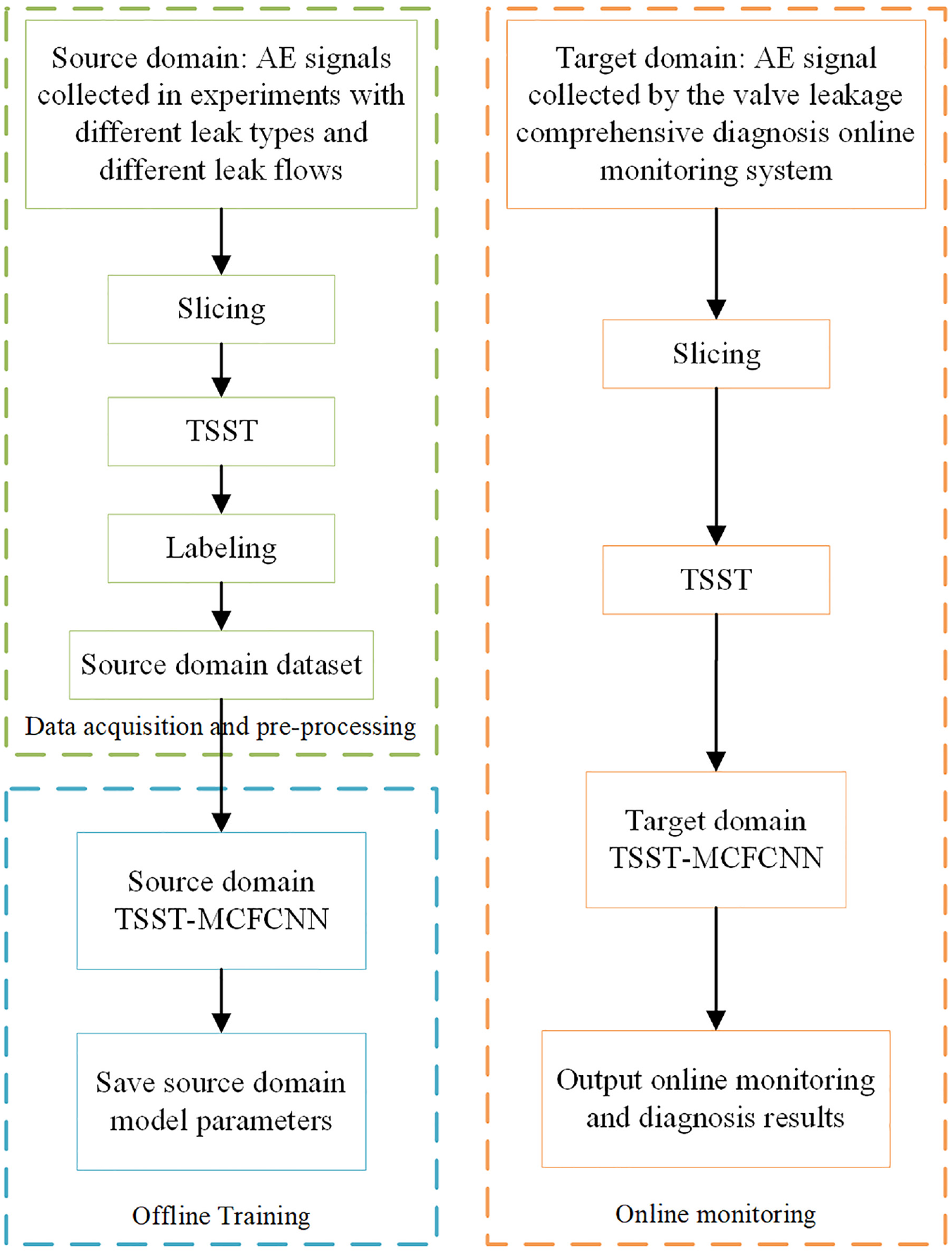
Schematic diagram of a comprehensive valve leakage diagnosis model.
Experiment
Experimental dataset
To validate the effectiveness of the comprehensive diagnostic model for valve leaks proposed in this article, an experimental platform for gas pipeline valve leaks was constructed, consisting of an air compressor, a gas storage tank, pipelines, pressure gauges, flow meters, test valves, and a testing system. Two test valves (DN40 ball valves) with sealing surface leakage and valve body leakage, respectively, as shown in Figure 5, were used to simulate internal and external valve leaks. During the experiment, AE detector (Soft-Island Times DS2, Beijing, China) was used to collect real-time leak AE signals, with a sampling frequency of 2.5 MHz. The AE sensor (Soft-Island Times G80, Beijing, China) had a resonant frequency of 80 kHz and was arranged on both sides of the test valve. The preamplifier had a gain of 40 dB and a bandwidth of 15 kHz–2 MHz to ensure signal amplification over the entire frequency band. During the experiment, high-pressure gas was pumped into the gas storage tank by the air compressor, and the system pressure was maintained at 0.5 MPa to simulate the stable backpressure of the valve. At this time, AE signals were collected for three conditions: internal valve leakage, external valve leakage, and no leakage. By controlling different leak flow rates, data for internal and external leaks ranging from 10 to 50 L/min were collected, greatly expanding the diversity of samples.
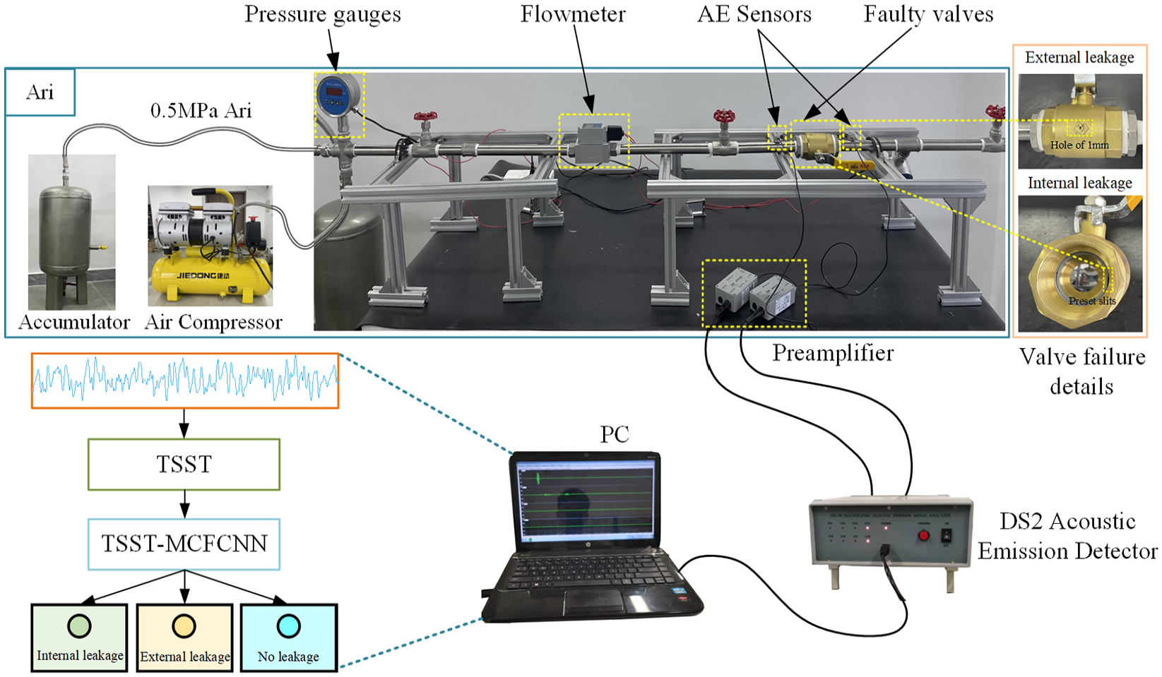
Experimental scenarios.
To validate the effectiveness of the model, AE signals were collected twice. The first set of data was used for model training and validation, whereas the second set was used for model testing. In the first data collection, a total of 16,000 AE signals were collected by the two AE sensors, resulting in 16,000 time–frequency images obtained using TSST. Following the principle of independent and identically distributed samples, the time–frequency images were divided into a training set of 12,000 and a validation set of 4000. In the second data collection, a total of 4000 AE signals were collected by the two AE sensors, and all 4000 time–frequency images obtained using TSST were used as the test set. The training set was used to learn the weight parameters w and bias b, the validation set was used to optimize the model parameters, and the test set was used to evaluate the model’s generalization ability. Before model training, the sample order of the training set was randomly shuffled to reduce model variance and alleviate overfitting. 30
Data preprocessing
The time-domain signals, frequency spectra, and TSST time–frequency images of the AE under the conditions of 10 L/min internal leakage, 40 L/min external leakage, and no leakage (including background noise) are shown in Figure 6. The frequency band of the internal and external leakage signals is mainly between 0 and 100 kHz, and their spectral similarity makes it difficult to directly identify the fault type. The internal leakage and no-leakage background noise signals exhibit similar periodicity in the time domain. Therefore, it is challenging to distinguish between internal leakage, external leakage, and no-leakage signals based on a single feature of the signal (such as frequency range, maximum amplitude, or maximum power).
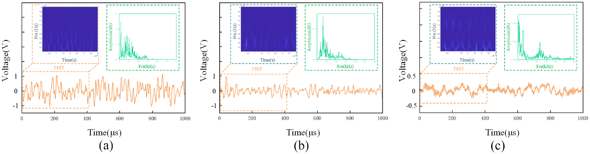
Valve leakage AE signal. (a) 10 L/min internal leakage of valve, (b) 40 L/min external leakage of valve, and (c) No leakage with background noise.
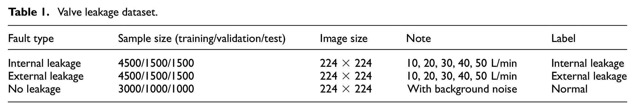
The present study detected two types of valve faults, internal leakage and external leakage. By comparing it with noise signals without leakage, it is verified that this method can quickly and accurately identify valve leakage failure modes in actual work scenarios. The corresponding fault categories and labels are shown in Table 1.
Valve leakage dataset.
Training of models
The real working environment of valve leakage is complex, and the measured AE signal generally contains strong background noise. This makes it difficult to obtain comprehensive fault characteristics if the signal measured by a single sensor, which can affect the accuracy of fault identification. In addition, the dangers posed by internal and external leakage failures of valves are different, leading to different emergency response options. Therefore, this article developed a TSST–MCFCNN for comprehensive valve leakage diagnosis, using TSST images from two sensors as input, which improves the accuracy and robustness of valve leakage diagnosis and can effectively distinguish between internal and external valve leakage faults.
The hyperparameters are one of the main factors that affect the generalization performance of a model. 31 The learning rate is an important parameter that controls the speed of gradient descent and affects the convergence of the model. If the learning rate is too small, the convergence speed will be slow, whereas if it is too large, the gradient will oscillate near the minimum, leading to convergence failure. Therefore, choosing an appropriate learning rate is crucial to improve the training efficiency and output stability of the network. The batch size is used to adjust the degree and speed of model optimization. In this article, the learning rate and batch size hyperparameters of the TSST–MCFCNN model were optimized through repeated experiments.
In order to mitigate the problem of overfitting, the ReLU activation function is employed. The Stochastic Gradient Descent with Momentum optimization algorithm 32 is utilized to regulate the learning rate of the network through the update of network parameters, with a validation frequency of 50. Furthermore, in order to prevent the overfitting of training data, the dropout regularization technique 33 is introduced in the fully connected layer at a rate of 50%. These measures have been shown to effectively enhance the performance of DL-based image recognition, as corroborated by previous research in the field.
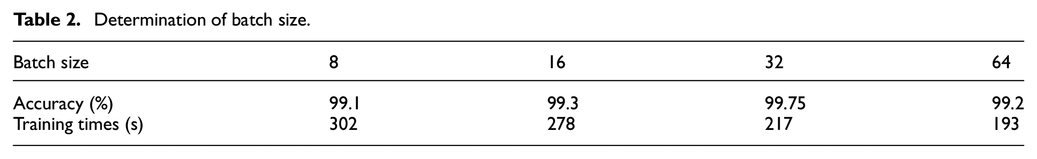
First, the model iteration number was set to 561, and the initial learning rate was set to 0.01. Then, the batch size was sequentially set to 8, 16, 32, and 64, and the experiment was repeated 10 times to take the average, evaluating the predictive performance of TSST–MCFCNN on the validation set. The training was done on GPU (NVIDIA GeForce GTX 1660 SUPER, Santa Clara, California, USA), and the platform was Windows 11 + Matlab2022a. The prediction results are shown in Table 2, which indicates that the valve leakage recognition accuracy is highest at a batch size of 32, reaching 99.75% with a computation time of 217 s. Although the training speed is slightly improved when the batch size is 64, the recognition accuracy is reduced. Therefore, considering both accuracy and computational cost, 32 is selected as the batch size.
Determination of batch size.
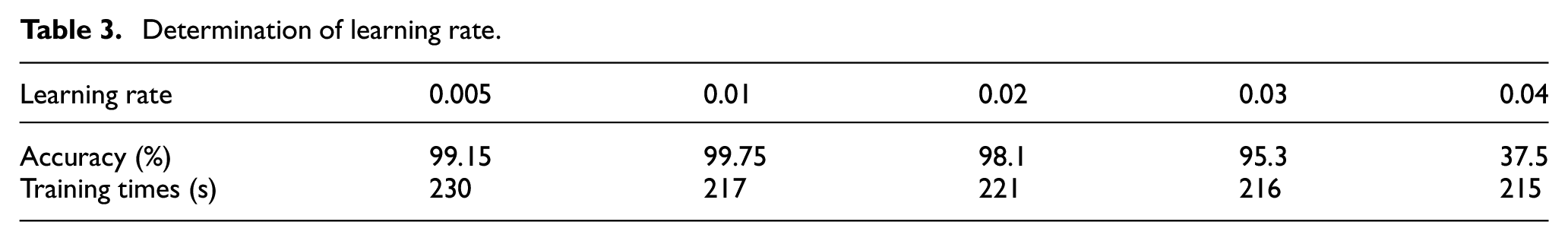
After determining the batch size, the learning rate was sequentially set to 0.01, 0.02, 0.03, 0.04, and 0.05, and the experiment was repeated 10 times to take the average, continuing to evaluate the predictive performance of TSST–MCFCNN on the validation set. The prediction results are shown in Table 3, which indicates that when the learning rate is set to 0.01, the TSST–MCFCNN model has the highest recognition accuracy. Therefore, the batch size and learning rate were set to 32 and 0.01, respectively, in this article.
Determination of learning rate.
Analysis of results
Performance comparison of different networks
In this article, artificial neural network (ANN) and traditional CNN are selected as the comparison methods for valve leakage fault diagnosis, and the average prediction accuracy on the test set is taken as the index by running each model 10 times to verify the superiority of the bi-sensor fusion method proposed in this article.
Locations results are saved after 561 iterations. CNN (single-sensor): TSST images from a single sensor are used as input, with the same structural parameters as the single CNN branch in TSST–MCFCNN, and the training results are saved after 561 iterations. ANN: The average, variance, energy, peak frequency, center frequency, pulse factor, and kurtosis factor of the leakage AE signal are utilized as features and inputted into a backpropagation neural network. For the BPNN, 7 neurons were selected for the input layer, 1 hidden layer was chosen with 128 neurons, and 3 neurons were selected for the output layer corresponding to valve internal leakage, valve external leakage, and no leakage. The activation function and learning rate were the same as the other two models, with ReLU chosen as the activation function and a learning rate set to 0.01, and the training results are saved after 561 iterations.
The average prediction accuracy of the various models is shown in Table 4. The proposed method achieved an average prediction accuracy of 99.85% on the test set, which represents a 19.05% improvement over the performance of the ANN model and an 8.3% improvement over the traditional CNN model. These results demonstrate that the proposed TSST–MCFCNN model has a significant advantage over both ANN and traditional CNN models for valve leakage fault diagnosis.
Accuracy of different models.
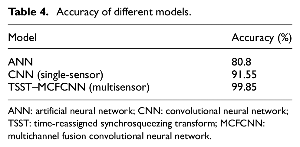
ANN: artificial neural network; CNN: convolutional neural network; TSST: time-reassigned synchrosqueezing transform; MCFCNN: multichannel fusion convolutional neural network.
The confusion matrices of the three models were analyzed, and the results are presented in Figure 7. The vertical axis of the confusion matrix indicates the actual labels of the samples, whereas the horizontal axis indicates the predicted labels of the samples. The ANN model incorrectly identified 20.2% of the no-leakage samples as valve internal leakage faults and 17.87% of the valve internal leakage samples as no leakage, indicating that the ANN model has difficulty distinguishing between these two cases. The CNN (single-sensor) model performed better than the ANN model, but it struggled to recognize samples in the no-leakage case, incorrectly identifying 24.2% of no-leakage samples as valve internal leakage faults. In contrast, the TSST–MCFCNN model achieved extremely high recognition accuracy, correctly identifying all valve internal leakage fault samples and no-leakage samples, and only 0.4% of the valve external leakage fault samples were misclassified. These results demonstrate that the TSST–MCFCNN model outperformed the other two models in classifying the three types of faults.
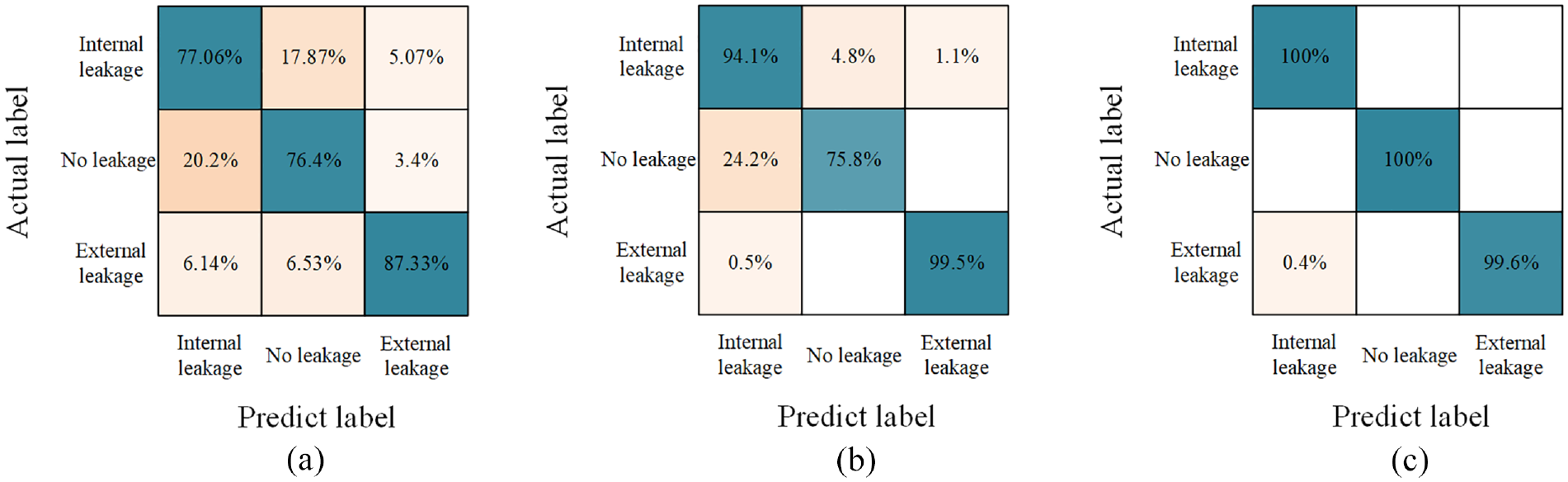
Confusion matrix for (a) ANN, (b) CNN (single-sensor), and (c) MCF–CNN models.
Effect of different time–frequency images on the model
Both STFT and TSST are methods for transforming time domain signals into the time–frequency domain. However, TSST is able to obtain a time–frequency representation with high-energy aggregation, whereas STFT cannot. This makes TSST more useful for distinguishing between the two types of valve faults: internal and external leakage. In this study, both STFT and TSST time–frequency images were used as inputs to MCFCNN, and the average prediction accuracy on various test sets (averaged over 10 runs) was used as the evaluation metric to compare the performance of STFT–MCFCNN with that of TSST–MCFCNN for comprehensive valve leakage diagnosis. The batch size was set to 32, the learning rate was 0.01, and the results were saved after 561 iterations.
The training curves of STFT–MCFCNN and TSST–MCFCNN (after Gaussian smoothing) are presented in Figure 8. The STFT–MCFCNN model exhibits a relatively slow convergence rate with some fluctuations during the training process, whereas the TSST–MCFCNN model converges faster and achieves higher accuracy during the training process.
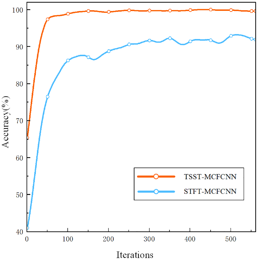
Training curves of STFT–MCFCNN and TSST–MCFCNN models.
On the test set, the STFT–MCFCNN model achieved an average prediction accuracy of 96.95%, whereas TSST–MCFCNN outperformed with an accuracy of 99.85%. The confusion matrix comparison between STFT–MCFCNN and TSST–MCFCNN is illustrated in Figure 9, revealing that TSST–MCFCNN is more effective in distinguishing between internal and external leaks. This is because these two types of faults are very similar in both the time and frequency domains, and accurate differentiation cannot be achieved solely based on the time–frequency information in the time–frequency image. The superiority of the TSST–MCFCNN model emphasizes the positive impact of clear modal information on identifying valve internal and external leakage faults.
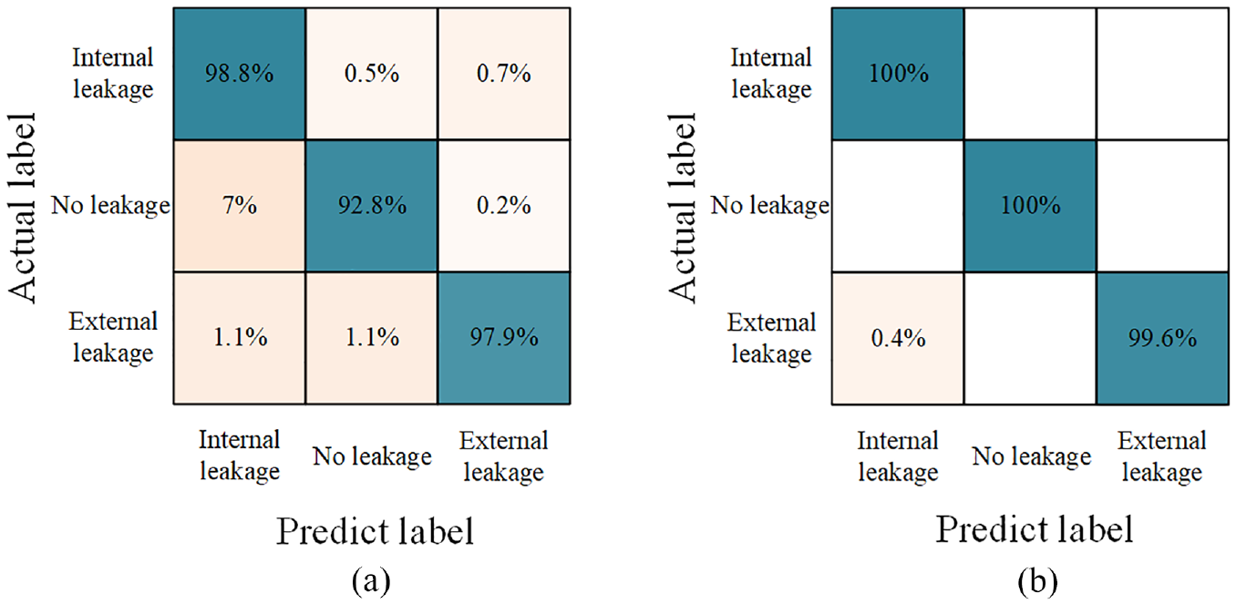
Confusion matrix for (a) STFT–MCFCNN and (b) TSST–MCFCNN models.
To better compare the classification performance of the STFT–MCFCNN and TSST–MCFCNN models, the t-Distributed stochastic neighbor embedding algorithm 34 was used to visualize the original input signal, the fully connected layer signal, and the model output signal in two dimensions for STFT and TSST, as presented in Figure 10. Figure 10(a) and (b) shows the original signals of STFT and TSST, respectively, where the different fault types are mixed and difficult to distinguish. The fully connected layer signals for STFT and TSST are shown in Figure 10(c) and (d), respectively, where the various fault types are largely separated and aggregated. The demarcation line of the TSST–MCFCNN model is more obvious, and the points where errors are clustered are marked with red boxes in the figure. Clearly, the STFT–MCFCNN model has more errors, and the identification accuracy is lower than that of the TSST–MCFCNN model. The model outputs are shown in Figure 10(e) and (f), where the TSST–MCFCNN model is more accurate and has a clear linear dividing line.
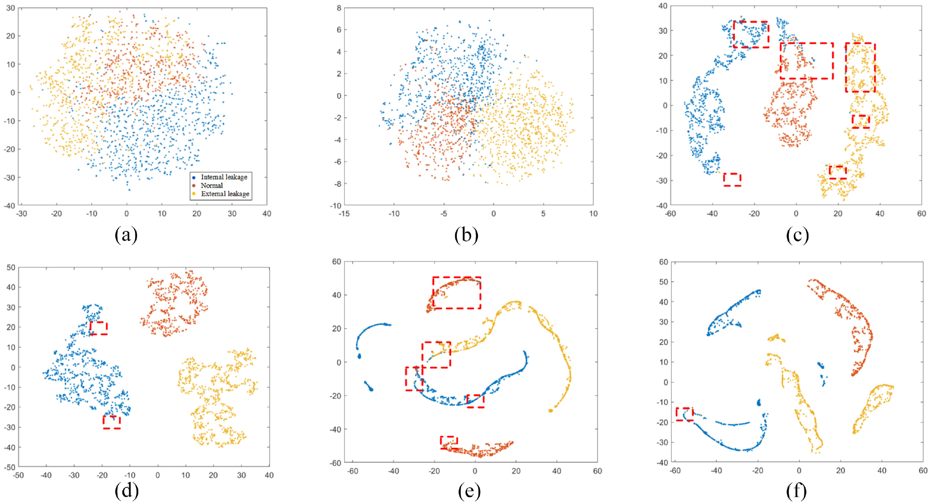
Two-dimensional visualization results of t-SNE. (a) STFT–MCFCNN-Input, (b) TSST–MCFCNN-Input, (c) STFT–MCFCNN-fc, (d) TSST–MCFCNN-fc, (e) STFT–MCFCNN-Output, and (f) TSST–MCFCNN-Output.
Effect of input sample sampling length on the model
The input of the model described earlier is a time–frequency image, which is obtained from a time-domain signal of length 1000 samples through TSST transformation. However, in online monitoring, a smaller sampling length means faster response speed and lower monitoring latency. This is of great significance for engineering practical applications. Therefore, this article studies the sensitivity of different models to the sampling length of input samples.
The performance of the STFT–MCFCNN and TSST–MCFCNN models were compared and analyzed using a time–frequency image containing 500 sampling points as model input. The average (run 10 times averaged) prediction accuracy of the STFT–MCFCNN model on the test set was 96%, which is a 0.95% decrease in prediction accuracy compared to a time–frequency image input of 1000 sampling points, and the average (run 10 times averaged) prediction accuracy of the TSST–MCFCNN model on the test set was 99.45%, which is a 0.4% decrease in prediction accuracy compared to a time–frequency image input of 1000 sampling points. The confusion matrix for the two models is shown in Figure 11. The ability of the STFT–MCFCNN model to identify two types of faults, internal and external valve leaks, is significantly reduced when the length of the sampled signals is reduced. However, the TSST–MCFCNN model maintained a high recognition accuracy.
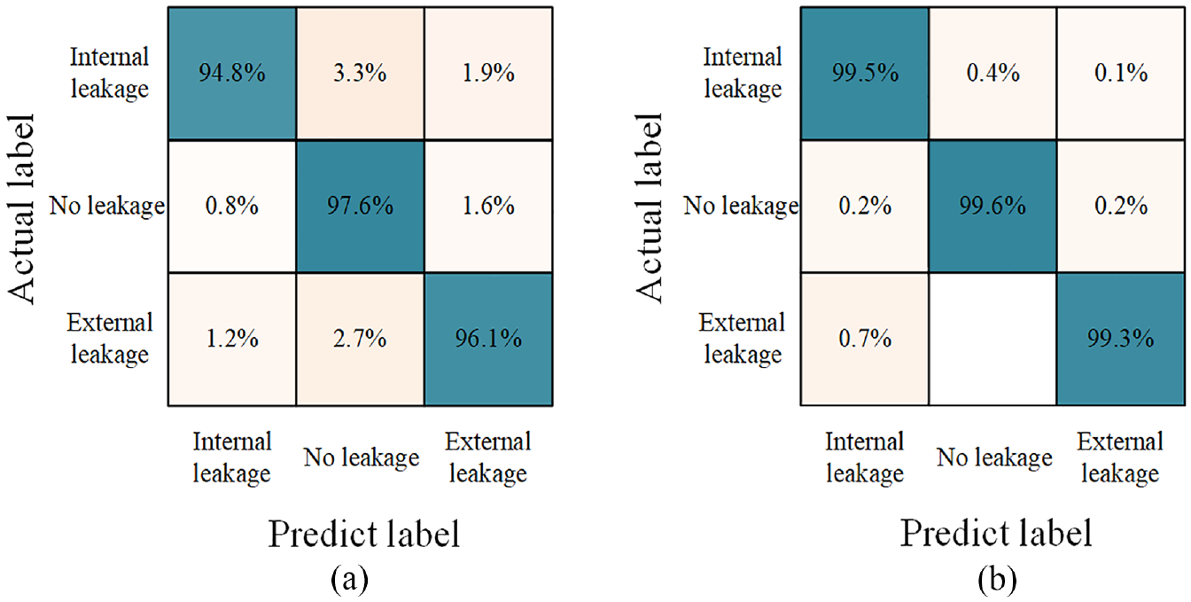
Confusion matrix for (a) STFT–MCFCNN and (b) TSST–MCFCNN models.
In addition, time–frequency images of 300 sampling points for both STFT and TSST are used as model inputs to evaluate their performance. The average (run 10 times averaged) prediction accuracy of the STFT–MCFCNN model on the test set was 94.25%, which represents a 2.7% decrease in prediction accuracy compared to a time–frequency image input of 1000 sampling points. The average (run 10 times averaged) prediction accuracy of the TSST–MCFCNN model on the test set was 98.8%, representing a 1.05% decrease in prediction accuracy compared to a time–frequency image input of 1000 sampling points. The prediction accuracy of different models with different sampling lengths is shown in Figure 12. As the input sample length decreases, the prediction accuracy of the STFT–MCFCNN model decreases faster than that of the TSST–MCFCNN model. The results show that compared to STFT–MCFCNN, TSST–MCFCNN required a shorter sampling length with the same diagnostic accuracy, which means that the method proposed in this study can achieve faster response time for ball valve leakage under conventional leakage flow rates.
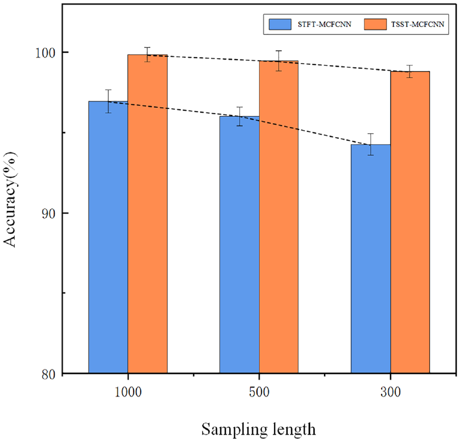
Prediction accuracy of STFT–MCFCNN and TSST–MCFCNN models.
Conclusion
In the field of valve leakage diagnosis, traditional methods have often focused on identifying a single type of fault, such as internal or external valve leakage, making them less effective in certain working scenarios. To address this issue, this study proposes a comprehensive valve leakage diagnosis model based on bi-sensor information fusion. Moreover, a novel comprehensive diagnosis method is introduced, which integrates time–frequency information, modal information, and position information of valve leakage. Two hyperparameters of the TSST–MCFCNN model, namely, the learning rate and batch size, were optimized using the valve leakage dataset, and the optimal values were determined to be 0.01 and 32, respectively. The performance advantages of the TSST–MCFCNN over ANN and traditional CNNs were experimentally verified, with an average prediction accuracy of 99.85% on the test set, representing a significant improvement over the ANN and traditional CNN by 19.05% and 8.3%, respectively.
Furthermore, the study investigated the role of modal information in distinguishing between two types of valve leakage faults, internal and external, using STFT and TSST time–frequency images as input to MCFCNN models. The results show that if the model contains clear modal information, it has a positive impact on the identification of these fault types. Finally, combined with practical engineering applications, the influence of sampling length is studied. Although the STFT–MCFCNN and TSST–MCFCNN models have different degrees of decrease in prediction accuracy after reducing the sampling length, the TSST–MCFCNN model accuracy decreases more slowly. Thus, the method proposed in this study can achieve faster response time for ball valve leakage under conventional leakage flow rates.
Footnotes
Declaration of conflicting interests
The authors declared no potential conflicts of interest with respect to the research, authorship, and/or publication of this article.
Funding
The authors disclosed receipt of the following financial support for the research, authorship, and/or publication of this article: This article is supported by the Fundamental Research Funds for the Central Universities (202165006), National Natural Science Foundation of China (52171283), and Natural Science Foundation of Shandong Province (ZR2020ME268).