Monitoring of material-removal mechanism in micro-electrical discharge machining by pulse classification and acoustic emission signals

Abstract

Micro-electrical discharge machining is a stochastic process where the interaction between the materials and the process parameters are difficult to understand. Monitoring of the process becomes necessary to achieve the dimensional accuracy of the micro-featured components. Although thermo-mechanical erosion is the most accepted material-removal mechanism, it fails to explain the material removal with very short pulse duration. Alternative postulate like electrostatic force-induced stress yielding provides a stronger argument, rising ambiguity over the material-removal process in the micro-electrical discharge machining regime. In this work, it was found that the stress waves released from the material during micro-electrical discharge-machining process indicate material removal by mechanical deformation and fracture mechanism. These stress waves were captured using the acoustic emission sensor. The discharge pulses were captured by voltage measurement and classified using voltage gradient and machining time duration into three major categories, open pulse, normal pulse and arc pulse. The acoustic emission signal features were extracted and identified by time–frequency–energy distribution analysis. A feed-forward back-propagation neural network mapping of the pulse instances was performed with the obtained acoustic emission signature. The time–frequency–energy distribution analysis of the acoustic emission and the scanning electron microscope images of the craters provide conclusive evidence that the material is removed by mechanical stress and fracture. The feed-forward back-propagation network model was trained to predict the discharge categories of the pulse instances with AE signal inputs which can be used for monitoring the material-removal mechanism in micro-electrical discharge machining operation.

Introduction

Micro-electrical discharge machining (micro-EDM) is a non-conventional machining process that uses electric discharge for material removal. Electric voltage (direct current or pulsating) is applied between tool and workpiece, kept at a gap, to produce discharges through a dielectric medium and small amount of material is removed at a time. In order to expand the machinability of the various materials as well as to increase the material-removal rate, many hybrid-variations of electrical discharge machining (EDM) process has been reported in the recent years like, ultrasonic vibration-assisted EDM, electrical discharge milling, electrical discharge grinding (EDG) and electrical discharge texturing (EDT) to name a few. These processes utilise the benefits of both conventional and unconventional material-removal process to overcome the limitations of the individual machining mechanisms. In the recent years, Zhang et al. ¹ proposed electrostatic field-induced electrolyte jet micro-EDM for silicon wafer. In the paper, the authors produced single-discharge between the tip of a fine jet of electrolyte (NaCl) and the workpiece (Si wafer) to remove the material. Micro-EDM is widely accepted in the manufacturing industry because the process is non-contact and capable of machining conductive materials irrespective of hardness. In a recent review, Prakash et al. ² extensively discussed the principles and mechanisms for both the conventional and micro-EDM process and brought out the present research trends, recent developments, advantages and gaps of the process. Unlike conventional EDM, micro-EDM is attributed with the absence of recast layer and barely produces heat-affected-zone for the micro-machined part. As reported by Mahdieh and Mahdavinejad, ³ conventional EDM produced recast layer ranging from 10 µm to 100 µm. The authors compared the thickness of the heat-affected zone (HAZ) as well as the recast layer between ultra-fine grained and coarse-grain aluminium alloy. On the contrary, Thao and Joshi ⁴ reported that recast layer was absolutely absent in the micro-EDMed surface. Although the authors had confirmed the thickness of the HAZ was between 30 µm to less than 100 µm. Micro-EDM is also ideal for drilling holes with ultra-high aspect ratios ⁵ and manufacturing micro-featured complex three-dimensional (3D) parts on difficult to machine materials. ⁶

The major drawback of the process is the stochastic behaviour that causes undesirable discharge instances like ‘arcing’ and ‘short-circuiting’ which damage the micro-features, increase the tool wear and interrupts the process. To address the inadequacies, Dauw et al. ⁷ proposed process-monitoring system for EDM through pulse classification by voltage level detection. The authors classified pulses by four main categories viz. ‘normal sparks’, ‘short circuits’, ‘arcs’ and ‘open circuits’ by a pulse discriminator algorithm (EDM-PD). Recently, Yeo et al. ⁸ used both voltage and current signals to develop pulse discrimination algorithm with adaptive servo control of the stage for maintaining a constant discharge gap. Zhang et al. ⁹ proposed a micro-EDM technology consisting of servo-feeding control strategy for micro-manufacturing of complex two-dimensional and 3D shapes. Mahardika and Mitsui ¹⁰ proposed a prognostic monitoring method of micro-EDM by relating several discharge pulses with the total discharge energy. Yan and Hsieh ¹¹ proposed an online process-monitoring system using gap voltage sensing and programmable logic controllers (PLCs) for controlling wire-EDM. Process monitoring in micro-EDM aims for stability during discharge. It is fundamentally monitoring the material-removal mechanism. Using acoustic emission (AE), the material-removal mechanism can be directly monitored, which is the most important part of micro-EDM to achieve quality control of the products.

The material-removal mechanism in the micro-EDM process is complex to understand because it is influenced by the interaction between the electrical, thermal, and chemical properties of the tool, the workpiece and the dielectric medium. The material removal for the EDM process can be classified into two broad categories ‘electro-thermal-erosion’ and ‘electro-mechanical’ mechanisms. According to the electro-thermal erosion mechanism, the electrical discharge produces heat flux across the tool gap, which melts and vapourises the tool and the workpiece to form a pool of molten material. The material from the melt-pool is removed through erosion caused by the flowing dielectric medium. DiBitonto et al. ¹² proposed an analytical model of the electro-thermal erosion mechanism by considering a point source heat model (PSHM) on the cathode (workpiece) which is taken as the benchmark model. Patel et al. ¹³ extended the work to develop a thermal heat flux model for anode (tool), and Eubank et al. ¹⁴ further extended it to develop the model for the electrical discharge considered as variable mass cylindrical plasma channel. Joshi and Pande ¹⁵ developed a numerical model of the cathode from the benchmark model. Shao and Rajurkar ¹⁶ developed a numerical model using the temperature distribution of the anode by Eubank et al. ¹⁴ The models considered electrical and thermal properties of the electrodes (constant case and time-varying case) and predicted the melt-pool radius (also called the crater radius). Mujumdar et al.^17,18 also proposed crater radius model with thermal heating and the forming of the melt pool. The authors also consider the chemical properties like the reactions in the plasma column and its interaction with the tool and workpiece surface. Joule heating is also considered as the thermal mechanism of the melt-pool formation. Marafona and Chousal ¹⁹ proposed a numerical model for crater depth by considering the melt-pool formation by Joule heating. Besides the finite-element models, the material-removal process is also researched using molecular dynamics (MD). Yang et al. ²⁰ used MD to simulate material-removal process in EDM and proposed that material removal happens either by vapourisation (associated with low power density) or by bubble explosion (associated with high power density) of superheated metals. The material-removal efficiency in the simulation was reported as 2%–5% which was very low. Recently, Yue and Yang ²¹ simulated EDM process using MD on polycrystalline as well as monocrystalline copper and compared the material dynamics behaviour. The authors concluded that polycrystalline copper has a large amount of HAZ, stacking faults, dislocations as well as larger crater diameter than monocrystalline copper. The electro-thermo erosion model relies on heat transfer from the discharge for melting and vapourisation of material. In contrast, for short-duration pulses, it raises the question if there is enough time for heat transfer to deliver the amount of heat required to melt the electrodes at all.

Although the MD simulations were based on thermal heat load, it suggests very low volume of material removal. Yang et al. ²² simulated the EDM process on copper using MD in a time order of few pico-seconds. The authors proposed that the residual stresses generated during EDM process is reason for the ablation and the bulge at the crater edge. The authors also computed the stresses and concluded that the shear stress may exceed the ultimate shear strength of the copper causing plastic flow of the material. This mechanism is a deviation from the conventional understanding of the material-removal process in EDM. Singh and Ghosh ²³ proposed an alternative material removal by mechanical deformation mechanism (referred to as electrostatic force-induced stress yielding) for short pulse duration (pulse duration for less than 5 µs). The applied voltage produces a discharge column that induces a localised electrostatic field on the material. The electrostatic force field induces stress on both the anode or cathode surface, causing yielding and failure. Such phenomena cause stress waves inside the material that can be detected as AE in the order of 100 kHz. Goodlet and Koshy ²⁴ reported the emission of AE during EDM and related it to monitor contamination of the electrode gap. Mahardika et al. ²⁵ used AE signals to detect the changes in the discharge energy during machining by micro-EDM. Smith and Koshy ²⁶ mapped the discharge height in a wire-EDM with the AE signals on the electrode and evaluated the spectrograms and power density. The time–frequency analysis of the AE signal brings out much-hidden information about the phenomenon. He et al. ²⁷ used Stockwell transform (s-transform) for monitoring of welding. The authors performed the axial tensile test on samples and captured the AE signature, which shows power consumption in a distinctive frequency range for each deformation stage. It was shown that the frequency range of AE signals for elastic deformation range below 100 kHz, for plastic deformation ranges between 100 and 200 kHz and for material fracture ranges between 100 and 400 kHz. Klink et al. ²⁸ mapped the process parameters of EDM with the AE signals and computed the amount of force exerted by the discharge. In this study, AE signal was released during the micro-EDM process, which indicates material removal by mechanical deformation. In order to relate the AE signal with widely accepted process monitoring by a pulse-classification algorithm, a feed-forward back-propagation (FFBP) artificial neural network (ANN) is used.

The application of ANN in EDM mainly involves the prediction of material-removal rate and surface roughness parameters. Pradhan and Das ²⁹ estimated the material-removal rate in EDM of AISI D2 tool steel using the recurrent neural network (Elman network) system. The authors proposed a model for material-removal rate in EDM with an error percentage of less than 6%. Pradhan et al. ³⁰ also proposed two models for predicting surface roughness parameters using ANN back-propagation network and ANN radial basis function network and made comparison between the two algorithms. The authors concluded that ANN back-propagation networks have better performance than radial basis function networks. Yadav and Yadava ³¹ used ANN for predicting material-removal rate and average surface roughness parameter for a unique hybridised process called slotted electrical discharge diamond grinding. The authors developed a hybrid technique by combining ANN and nondominated sorting genetic algorithm to optimise the process parameters. In the present work, back-propagation technique has been used to study the relationship of material-removal mechanism with the duration of the pulses.

The objective of the study is to establish a map between the pulse categories and the AE signals emitted during micro-EDM and to determine the AE signal features that are contributing significantly towards the classification of the pulse train. In this article, the discharge pulses captured during the micro-EDM process were classified into three classes, viz. open pulse, normal pulse and arc pulse as well as the AEs released during machining were mapped to these categories of pulses. The discharge pulses were classified by the machining time of each pulse, estimated by the voltage gradient method. The machining time for a discharge pulse was calculated by the summation of the rise time, ignition delay period and the discharge duration for each pulse. The AE signal features like strength of the signal, frequency, and power spectral density (PSD) were estimated for the captured data. Time-spectral features like energy spectrograms, intrinsic modal functions (IMFs) extracted by empirical mode decomposition (EMD) transformation of AE data were also determined. These temporal features were correlated by ANN model to the discharge instances. An FFBP neural network was constructed with the selected features as input data and the classified pulse categories as the output data. The network was trained and tested on independent sets of data. The network was evaluated based on its performance, training state, error and the confusion matrix. It establishes a relationship of the AE data to the classified pulse categories, which provides a deeper understanding of the material-removal mechanism in the corresponding discharge class.

Experiment and methodology

The micro-EDM process produces discharges with varying durations of plasma channel, which have different plasma-material interaction mechanisms like melting-vapourisation-erosion, plastic failures, and micro-fractures. Hence, monitoring the material-removal mechanism is necessary for consistently achieving the discharge duration that removes the material in the desired manner. Material removal through melting-vapourisation happens for plasma-material interaction in long-duration pulses. In contrast, the plasma produced during short-duration pulses does not have enough time for heat transfer to cause melting and vapourisation process. The present work hypothesises that the short-discharge pulses remove the material by mechanical deformation and fracture mechanism. Since material deformation and fracture produces stress waves as AEs. The hypothesis has been investigated by analysing the AE signals during the discharge process and simultaneously classifying the discharges into ‘open’, ‘normal’ and ‘arc’ pulses. Figure 1(a) shows the demonstration of the concept and the methodology. In the figure, the electrical discharge is producing stress waves in the form of AEs. The AE sensor picks up the signals and amplifies it. The oscilloscope captures the AE signals, pulse generator voltage, gap voltage and the discharge current simultaneously. These signals were post-processed to detect the pulse durations, classify them and to extract the AE features. As discussed in section ‘Time–frequency–energy study of the AE signal’, micro-electrical discharges produce distinct AE signatures during the elastic deformation, plastic deformation and fracture of the material. Thus, the proposed method helps to monitor the material-removal mechanism by each discharge instance and to know whether the material removal is purely by melting and vapourisation or through fracture mechanism.

Figure 1.

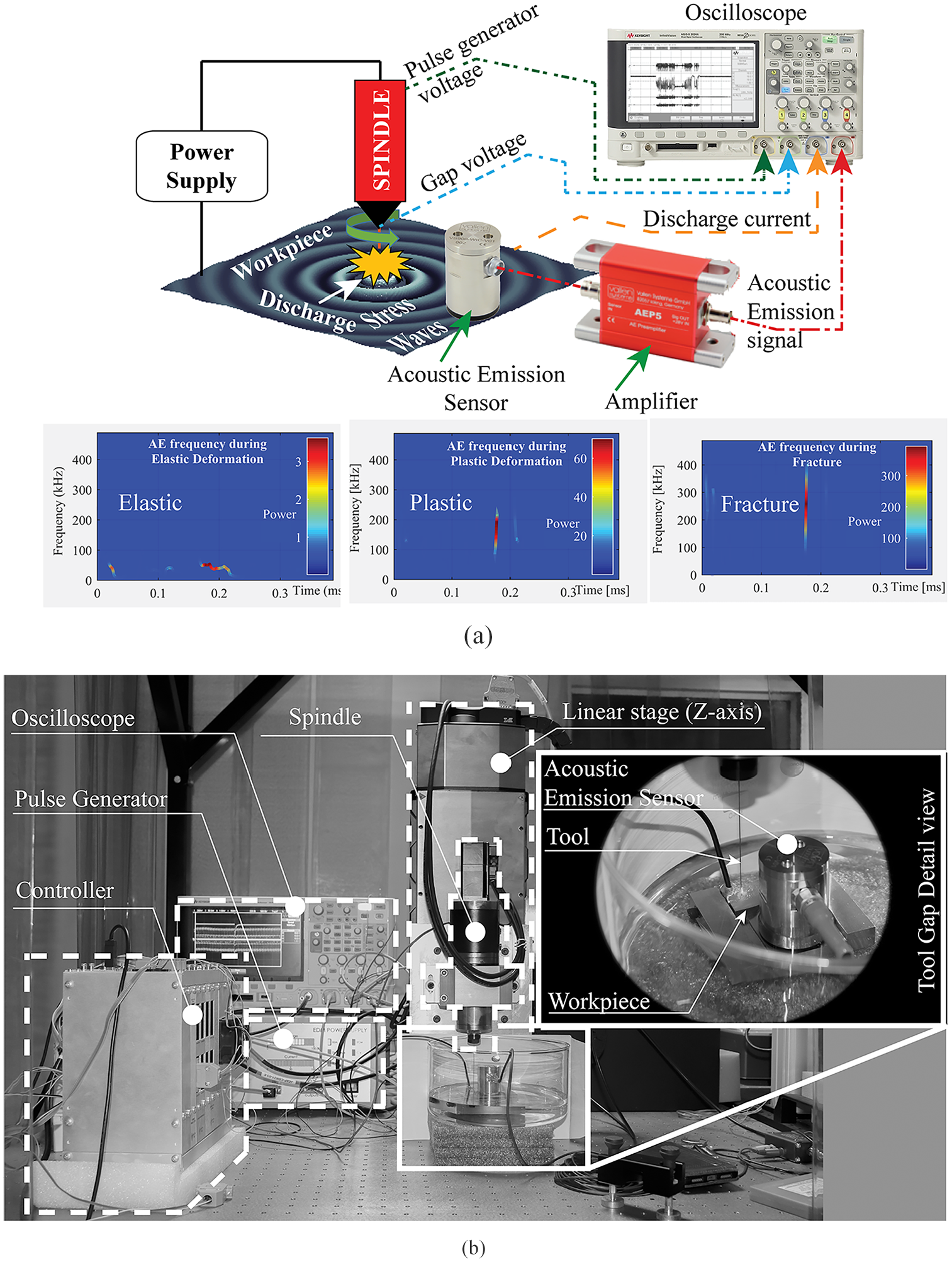
Concept illustration and experimental setup: (a) demonstration of the concept and methodology and (b) the micro-EDM setup.

Experimental setup

The micro-EDM setup used for the experiments is shown in Figure 1(b). It consists of a resistor–capacitor (RC)-based pulse generator manufactured by Mikrotools with voltage ranging from 80 to 140 V with resistance 1 kΩ and six selectable capacitance range from 10 pF to 400 nF. A linear stage for Z-axis movement manufactured by PI LS180, with 10 µm precision in movement was utilised. AC servo motor with maximum speed 3000 r/min, manufactured by Yoshikawa, was used as the spindle for the tool rotation. A six-axis controller manufactured by Delta-tau (model TurboUMAC) was used for the control of the process. Deionised water (DI water) was used as a dielectric medium. A 0.5 mm diameter copper tool was used on 2 mm thick titanium (Ti-6Al-4V) workpiece.

The detailed view of the tool gap in Figure 1(b) shows AE sensor manufactured by Vallen Systeme Gmbh, Germany. The bandwidth of the sensor is from 100 to 900 kHz and has a preamplifier with a gain of 34 dB. The sensor calibration certified underwater performance in the operational bandwidth. DSO 2024A Keysight Technology oscilloscope, bandwidth 200 MHz and a maximum sample frequency of 2 GSa/s was used for measurement of the signals and the pulse trains. The oscilloscope was used for measurement of AE signal, gap voltage, discharge voltage at the pulse generator output and discharge current.

The experiments were performed with the discharge voltage as 80, 120 and 140 V and the discharge capacitor of 400 nF. The time constant of the circuit was calculated as 4 µs. The ideal discharge was considered for a duration of 10 µs.

Pulse classification and features detection

The signals obtained from the oscilloscope are post-processed in MATLAB R2018a for analysis. The pulse classification and the AE feature-extraction programmes are scripted in MATLAB editor. First, the gap voltage data are imported to detect the pulses on the basis of a trigger voltage. Then the pulse train is scanned in the time to determine machining time, and the duration of each pulse is estimated. For each pulse, the rise time, delay time and the discharge time are detected based on the gradient of the gap voltage. Rise time is calculated for the duration of the gradient is more than 1.5 V over 20 µs. The ignition-delay period is calculated for voltage gradient between 0 and 75 mV/µs, and the discharge duration is calculated if the voltage gradient is negative. These three discharge phases are added to determine the total machining time of the single pulse. Figure 2(a) shows that the captured gap voltage pulse superposed with the machining time detected by the algorithm. Figure 2(b) shows the detailed view of 120 µs of the voltage data where two pulses are detected and the estimation of rise time, delay time and discharge time are plotted. This sequential detection process of the phases of the gap voltage train, that is, rise time, ignition delay time and the discharge time, demarcates the end of each pulse.

Figure 2.

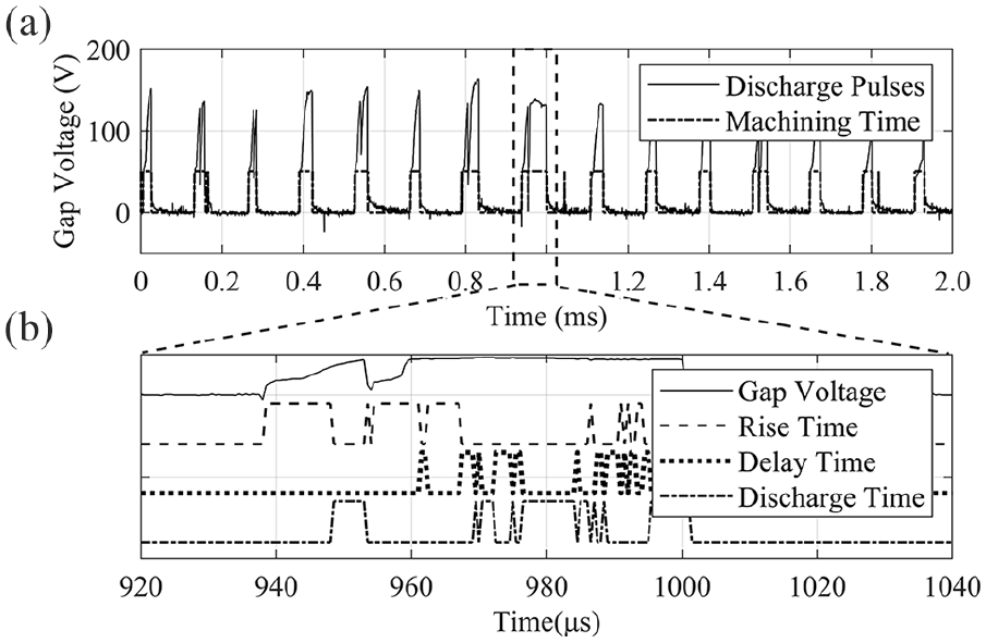
Detection of the pulse and estimation of machining time for each discharge pulse: (a) pulse train series and detected pulse and (b) details of the pulse phases during discharge.

After the detection of the machining time by the voltage-gradient method, each pulse was categorised under three categories as ‘open circuit’, ‘normal pulse’ and ‘arc pulse’ based on the machining time compared to the ideal pulse. The ideal pulse duration is considered as 10 µs for all the analysis. A discharge capacitor of 400 nF was used during the experiments. Figure 3 shows the counting and classification of pulses from the captured gap voltage. As shown in Figure 3(a), the captured gap voltage is plotted. As shown in Figure 3(b), the pulse classifier detects pulses of various duration, cumulating to 32 pulses. Each of the detected pulses is categorised into three classes, viz. ‘open pulse’, ‘normal pulse’ and ‘arc pulse’ by comparing the machining time of each pulse to the ideal discharge duration, shown in Figure 3(c)–(e), respectively.

Figure 3.

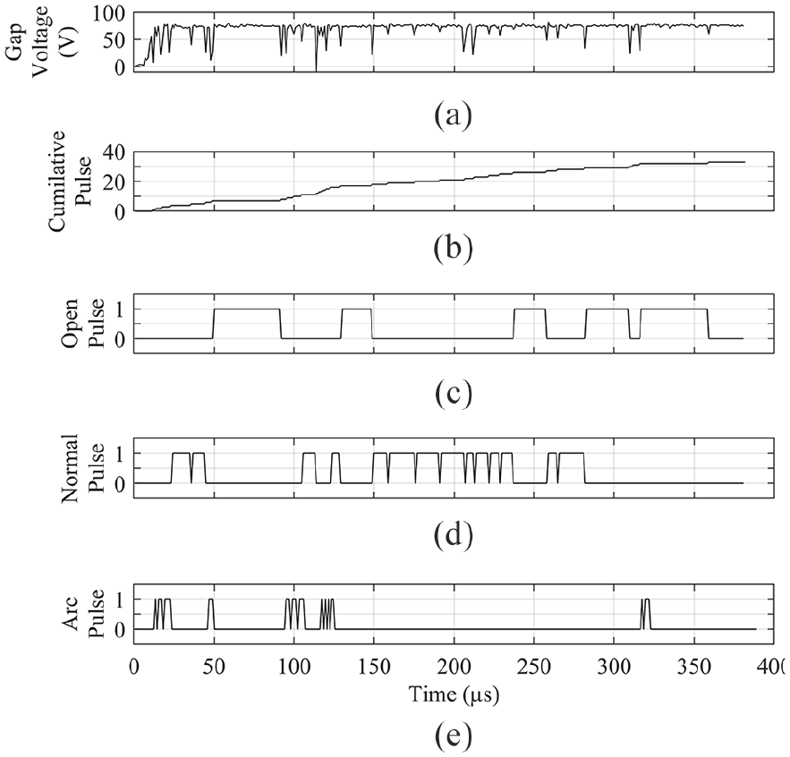
Counting and classification of pulses into open normal and arc pulses for 32 discharges: (a) gap voltage plot, (b) cumulative pulse count and (c)–(e) are the plot of time-series data for ‘Open’, ‘Normal’ and ‘Arc’ pulse, respectively.

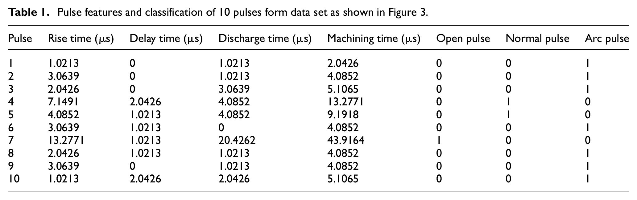
The selected features, ‘rise time’, ‘delay time’ and ‘discharge time’ are the attributes to the pulse quality, which becomes the primary basis of the classification of the pulses. Table 1 shows a set of 10 pulses, their features and classifications from a pulse train data set. These classified pulses are used as a target data to train and test the ANN, which takes the AE signal features as the input, discussed in section ‘ANN’.

Table 1.

Pulse features and classification of 10 pulses form data set as shown in Figure 3.

Pulse	Rise time (µs)	Delay time (µs)	Discharge time (µs)	Machining time (µs)	Open pulse	Normal pulse	Arc pulse
1	1.0213	0	1.0213	2.0426	0	0	1
2	3.0639	0	1.0213	4.0852	0	0	1
3	2.0426	0	3.0639	5.1065	0	0	1
4	7.1491	2.0426	4.0852	13.2771	0	1	0
5	4.0852	1.0213	4.0852	9.1918	0	1	0
6	3.0639	1.0213	0	4.0852	0	0	1
7	13.2771	1.0213	20.4262	43.9164	1	0	0
8	2.0426	1.0213	1.0213	4.0852	0	0	1
9	3.0639	0	1.0213	4.0852	0	0	1
10	1.0213	2.0426	2.0426	5.1065	0	0	1

AE signal features extraction

It was observed during EDM that AE signal bursts occur during the process. As shown in Figure 4, the signal bursts are in the form of impulses at a specific time instant. The objective is to study the signal features and correlate them with the classified pulse. The identified features are the signal voltage, the frequency as well as the phase of the AE signal, the PSD and time–frequency–energy parameters. Since the AE signal generated during the discharge is a non-stationary signal, that is, its frequency components changes with time, a deeper spectral analysis is required for capturing the distinctive features. An EMD analysis by decomposing the AE signal into the IMFs is performed and a few significant IMFs are selected as AE features. Finally, the analysis helps us to select nine features as a function of time, the signal strength, frequency and phase of the signal, power of the signal, spectral energy of the signal and four significant IMFs. These signal attributes along with the gap voltage become the input layer of the neural network model.

Figure 4.

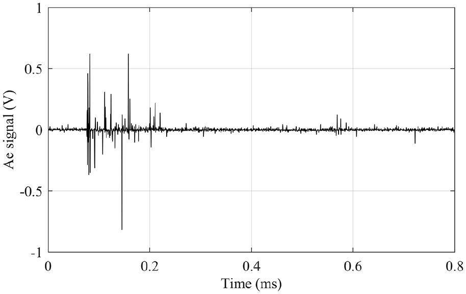
AE signal during discharge.

The fast Fourier transformation (FFT) of the AE signal bursts is shown in Figure 5. The frequency amplitude plot as shown in Figure 5(a) does reveal peaks. The phase–frequency plot (Figure 5(b)) shows that there is a gradual phase shift from the positive side to the negative side, over the peak frequencies around 100, 150, 200, 250 and 350 kHz. It can be inferred that there is a change in the values of the power of the signal at these frequencies. As mentioned earlier, the AE signal bursts are non-stationary signals, we cannot estimate the power of the signal, instead, we would estimate the energy. The signal power and the energy are interchangeable for a non-stationary wave.

Figure 5.

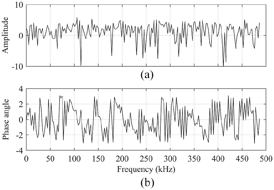
Frequency plot of the AE signal: (a) amplitude and (b) phase angle.

For further exploration, the trend as shown in the phase–frequency plot (Figure 5(b)) of the PSD of the signal is estimated at various frequencies. Figure 6 shows the PSD estimation of the AE signal data series collected during the discharge. The PSD was performed with 32 sample point window and 16 sample point overlap with 128 discrete Fourier transformation (DFT) points. Hamming window is used for windowing each segment. It can be seen from the plot that distinctive peaks of the signal at 103, 190.8, 281.6 and 366.4 kHz locations. In and around these frequencies, the maximum power of the signal is perceived. We have carried out the PSD analysis for more data sets, and observed consistent peaks in and around these frequencies. The peak frequency values of the PSD for the data sets are given in Table 2. It can be implied that the energy is transferred from the discharge to the material at certain frequency ranges.

Figure 6.

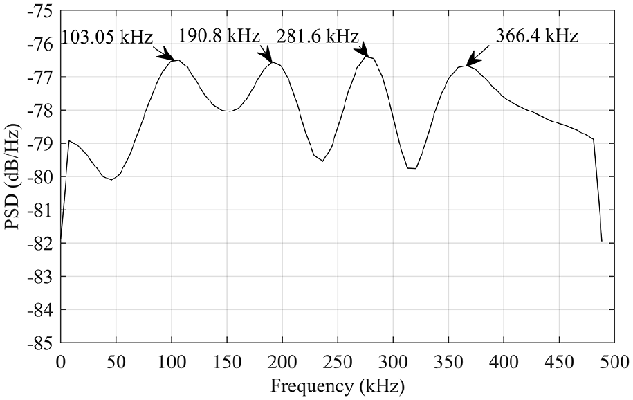
Power spectral density (PSD) of the AE data showing four peaks of DS4 in Table 2.

Table 2.

PSD peaks for different data sets.

Sl. no.	Datasets(DS)	PSD peak frequencies (kHz)
1	DS1	53.43, 137.4, 259.5, 320.6, 404.6, 480.9
2	DS2	99.2, 152.7, 213.7, 281.6, 377.5, 458.0
3	DS3	68.7, 129.8, 198.5, 259.5, 328.2, 396.9, 442.7
4	DS4	103.5, 190.8, 281.6, 358.8
5	DS5	61.07, 129.8, 137.4, 213.7, 320.6, 396.9, 480.9
6	DS6	175.6, 251.9, 328.2, 404.6, 480.9

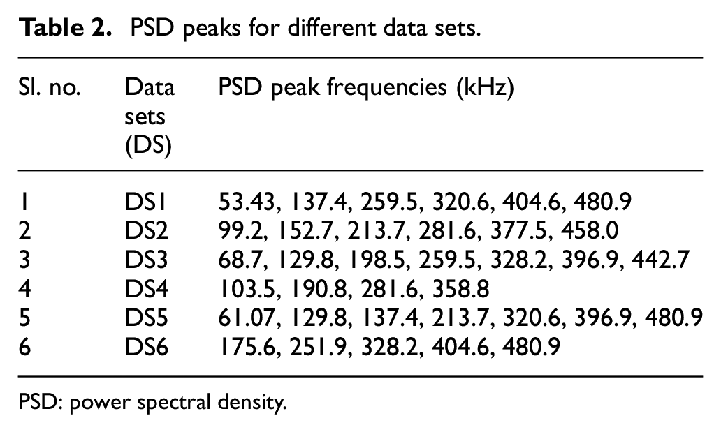
PSD: power spectral density.

ANN

ANN is a computational model inspired by, how the nervous system relates the stimuli with the reactions, by transmitting neuro-signals from one biological neuron to the other. Figure 7(a) shows a single-input neuron that represents the simplified mathematical model of the neuro-transmission process in a biological neuron. The input signal (p) represents the incoming neuro-signal transmitted across the synapse (junction between nerve cells) that overcomes the gap. The signal transfer depends on the strength of the synapse (w), the bias of the neuron (b), and the cell body, represented by the summation and the activation function (f). The output signal (a) represents the neuro-signal in the axon. The chosen learning rule adjusts the parameters w and b. The authors have considered the back-propagation algorithm for learning.

Figure 7.

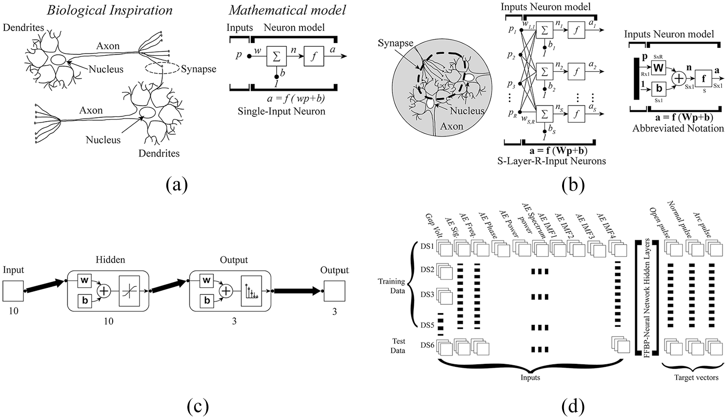
Feed-forward back-propagation (FFBP) neural network with input output variables: (a) single-input neuron model, (b) S-layer neurons, (c) FFBP neural network for pattern recognition and (d) the matrix of input and output variables for various data sets (DS) of training and test data. (Here, p is the input signal in the Dendron, a is the output signal at the axon, b is the bias of the neuron, w is the weight corresponding to the strength of the synapse, n is the intermediate summation of signals, and f is the activation function of the synapse.).

The relationship between the inputs and outputs becomes complicated when multiple neurons are interacting. Figure 7(b) describes a layer of S neurons with R inputs. Here, the input vector (p), consisting of R number of input signals (p₁, p₂,…, p_R) are connected to S neurons with individual weights (w_1,1, w_1,2,…, w_S,R) forms the weight matrix (W). Each of the neurons has a bias (b₁, b₂,…, b_S) which collectively forms the bias vector (b). These vectors are added to form the intermediate vector (n), which is multiplied by the activation function vector (f). Hence, the output vector is computed as

$$\mathbf{a}=\mathbf{f}(\mathbf{Wp}+\mathbf{b})$$

(1)

As shown in Figure 7(c), the abbreviated network representation has been used for the hidden layers of the developed network. The number at the bottom of the block indicates the number of hidden layers.

An FFBP neural network model was used to establish a map between the classified pulses and the gap voltage as well as the AE signal along with its derivative parameters. Neural network toolbox by MATLAB was used. The network, as in Figure 7(c), has 10 hidden layers and three output layers. A hyperbolic tangent sigmoid function (tansig) was used as transfer function (the activation function) of the hidden layer neurons, and normalised exponential function (softmax) was used for the classification neurons. As shown in Figure 7(d), the gap voltage signal and AE features like AE signal, frequency, phase, power, spectral energy, IMF1 through IMF4, total of 10 variables were taken as the input for the network, and the pulse classes, that is, the ‘open’, ‘normal’, and ‘arc’ pulses are the three target vectors. Five data sets, denoted by DS1–DS5 of varying sizes of data, were selected for training of the network and was tested on another independently captured data set DS6. Random indices were used on the target data and separated into training, validation and the testing data with the distribution of 70%, 15% and 15%, respectively. Back-propagation learning by scaled conjugate gradient (SCG) algorithm was used for training the network, and cross-entropy was evaluated for performance criterion. The cross-entropy algorithm heavily penalises extremely inaccurate results and awards very little penalty for nearly correct classifications. Thus minimising cross-entropy generates better classifier.

Results and discussion

Time–frequency–energy study of the AE signal

The time-series data gives information about the events that occur in sequence. As discussed earlier in section ‘AE signal features extraction’, that AE signal occurs in bursts, but not all the discharges detected from the gap voltage produce the same power of the AE signal. It is a fact that, AE signal attributes crack-propagation inside the material. As mentioned, not all discharges remove the material in the same mechanism. So it becomes important to study the sequence of the discharge classification while correlating with the AE. In this section, the time–frequency–energy analysis of the AE data is discussed, that is, how the energy of the AE signal is distributed over the temporal and spectral domain.

An intuitive understanding of the concept that different discharges produce AE with variation in power can be seen from Figure 8. It shows the time trace of the gap voltage where the discharge is clearly seen as vertical drops in voltage, shown in Figure 8(a), and the short-time Fourier transform (STFT) of the AE signal corresponding to the same data for the same duration, shown in Figure 8(b). It is quite evident that the series of discharge pulse produces the different powers of signal over various frequency–time domain. In Figure 8(b), the colour-coded values represent the energy of the AE signal, Y-axis is the frequency, and X-axis is time. The spectrogram is constructed by taking 32 sample points of the AE signal, with 16 sample overlap points and 128 DFT points. It can be seen in the spectrogram that the highest value of the power is transferred between the 0.2 and 0.6 ms of the signal. A neural network map between the counting and classification of pulses (Figure 3), and the spectrogram data are already discussed in section ‘ANN’.

Figure 8.

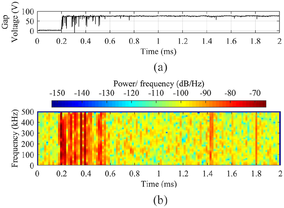
Time–frequency–energy study: (a) gap voltage during the discharge and (b) short-time Fourier transform (STFT) analysis of the acoustic emission data.

In order to understand the ranges of spectral components with a significant amount of energy in the AE signal, an EMD analysis is performed. The AE signal is decomposed into nine nearly orthogonal components called intrinsic mode functions (IMFs). Although the signal can be decomposed into more number of IMFs, the residual of less than 0.0001 is considered as the stopping criterion. The values of nine IMF parameters are shown in Table 3. The AE signal, along with first five IMF and the residual is plotted, as shown in Figure 9. It can be seen that the amplitude and the frequency components of the IMF are decreasing from IMF1 through IMF5. In order to select the significant IMF, the energy of each IMFs is evaluated. ( $\mathrm{Energy}={\int }_{-\infty }^{\infty }|x(t){|}^2\mathrm{dt}$ where x(t) is the signal. It is a relative measure of the energy.) The total significance percentage of energy from IMF1 to IMF4 constitutes of 94.99% of the original signal. IMF5–IMF9 put together constitutes of 5.01% energy of the original AE signal. Hence, the IMFs with energy less than 0.1 that contributes to less than 5% to the energy information of the original signal are considered insignificant.

Table 3.

Intrinsic mode function parameters.

Sl. no.	Signal	Residue	Energy	Extrema	Zero cross	Significance percentage
1	AE Sig.	–	3.3190	–	–	100
2	IMF 1	0.0549	2.1195	1206	1200	63.86
3	IMF 2	0.0723	0.5888	564	553	17.74
4	IMF 3	0.1321	0.2851	267	263	8.59
5	IMF 4	0.0419	0.1592	126	123	4.80
6	IMF 5	0.0523	0.0845	62	63	2.59
7	IMF 6	0.0376	0.0450	31	26	1.38
8	IMF 7	0.0549	0.0279	11	11	0.86
9	IMF 8	0.0182	0.0083	6	6	0.26
10	IMF 9	0.0803	0.0007	4	3	0.02

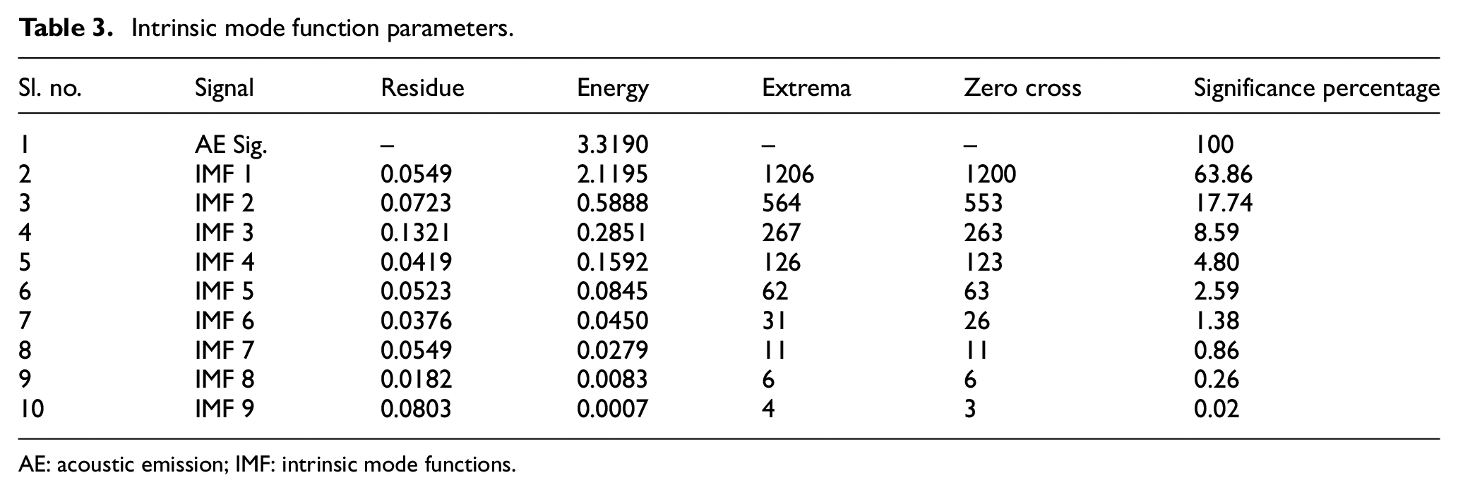
AE: acoustic emission; IMF: intrinsic mode functions.

Figure 9.

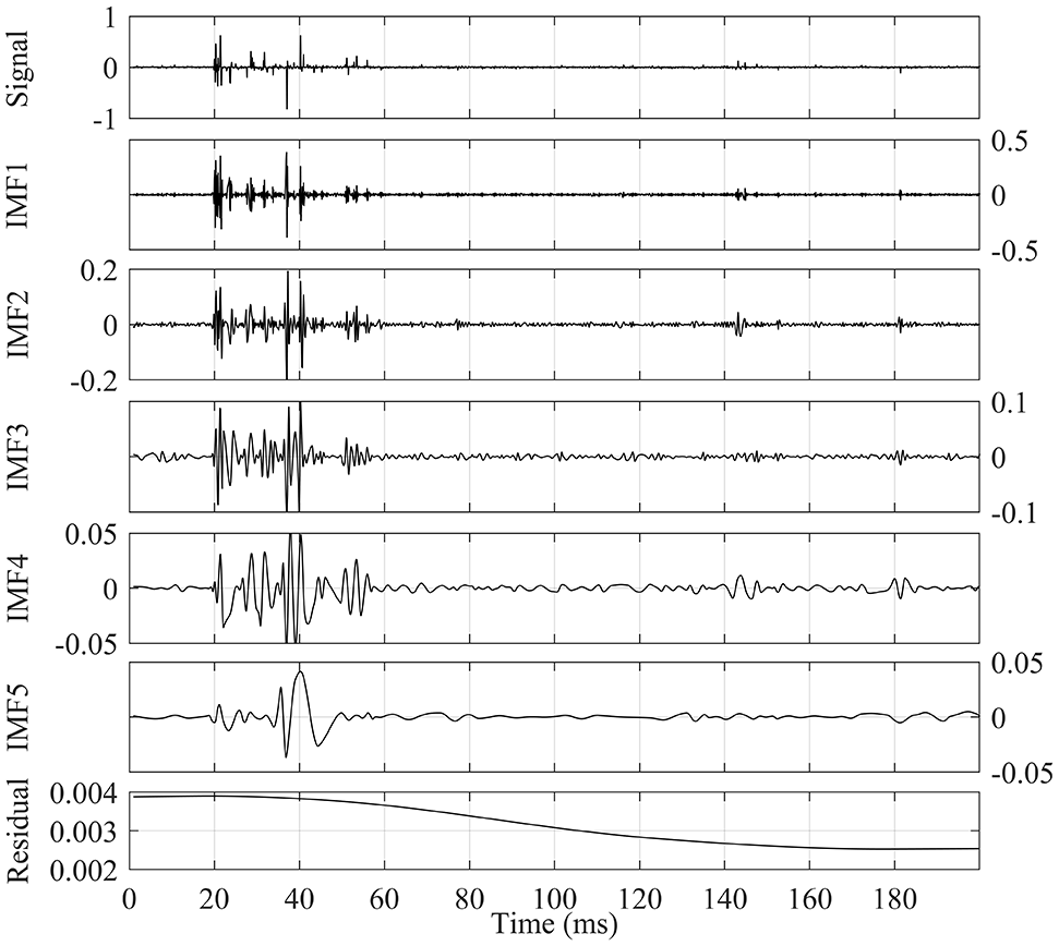
Empirical mode decomposition of the AE signal into intrinsic mode functions (IMFs).

Now the non-stationary complicated AE signal is decomposed into the IMFs that contain the information of the material-removal mechanism. The spectral decomposition of each IMF provides the information, which frequency components (corresponding to fracture, plastic and elastic failure) contain how much amount of power at a given time instant. This is better comprehended in the Hilbert–Huang transformation (HHT) plot, as shown in Figure 10. The frequency component between the 100 and 400 kHz, for IMF 1, carry most of the power, with a maximum energy around 250 kHz at 0.18 ms, as in Figure 10(a). The frequency range suggests material fracture mechanism. Hence, IMF 1 corresponds to the fracture failure of the material. HHT of IMF 2 shows the energy consumption between 100 and 250 kHz with maximum power around 150 kHz, suggesting material removal by plastic deformation, as shown in Figure 10(b). Similarly, IMF 3 and IMF 4, as shown in Figure 10(c) and (d), respectively, provides the energy–frequency–time information having frequency less than 100 kHz, which suggest melting or elastic deformation process. It can be observed that the signal power is decreasing at the lower-frequency IMFs, which suggests reduced tendency of mechanical removal process. In other words, the lower energy for IMFs indicates lower chance of mechanical failure process and higher chance of material removal by thermal failure. These four IMFs, since they correspond to unique mechanisms of material removal, are considered as the inputs for the neural network map.

Figure 10.

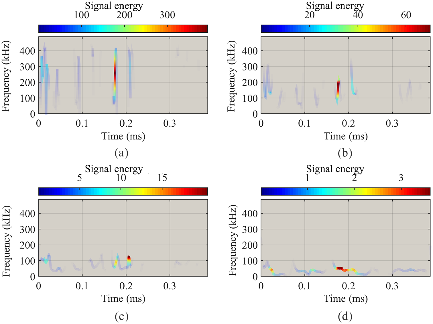
Hilbert–Huang transformation plot for (a) IMF 1 showing fracture failure, (b) IMF 2 showing plastic failure, (c) IMF 3 and (d) IMF 4 showing elastic deformation and melting and vapourisation process.

ANN performance

After the pulse classification, discussed in section ‘Pulse classification and features detection’, the categorised pulses are required to be in time-series data format. As in Table 1, the pulse train features and the pulse classification are enlisted on each detected pulse but the data are not temporal. The time-stamp of the data was achieved by segregating the cumulative pulses into three arrays of same length (as the cumulative data length), each corresponding to the class of the pulse. As shown in Figure 3(c)–(e), the pulse arrays are the function of time. Thus, the target network data set consisting of three vectors has the same time-stamp as the input data.

The best validation performance was achieved with the cross-entropy value 0.10562 at epoch (iteration) 56. As shown in Figure 11, the network performance remains almost constant cross-entropy value of 0.0954 until epoch 62. The stopping criterion for training the network was taken as six validation checks. Figure 12(a) shows the training state of the network and plots the gradient values for SCG algorithm against each iteration. The graph shows a good convergence in the gradient. Figure 12(b) describes number of the validation fails for each epoch, and the plot ends with six validation checks.

Figure 11.

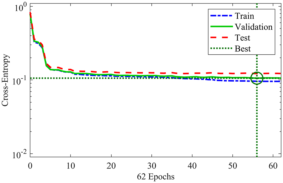
Network performance by cross-entropy.

Figure 12.

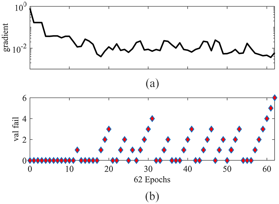
Network training state: (a) gradient = 0.0060916, at epoch 62 and (b) six validation checks, at epoch 62.

The tally of the network on the test data set is shown in Figure 13. In Figure 13(a), the error histogram plot shows error magnitude and number of times it occurs. It can be seen that there are nearly 150 instances (maximum) with the error of −0.05. The confusion matrix as shown in Figure 13(b) shows the overall prediction percentage of the target classes, the right bottom corner of the matrix, is 66.4% correct and 33.6% incorrect predictions. The percentages in green denote the correct and the red denotes the incorrect. The first three elements of the fourth row of the matrix show the total predicted percentages for each class and the fourth column of the matrix corresponds to the percentage of target classes.

Figure 13.

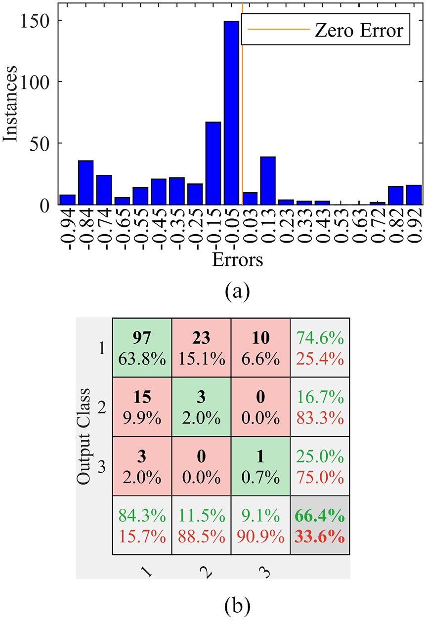
Error histogram and confusion matrix: (a) error histogram of the network and (b) confusion matrix for three classes. Class 1, 2, 3 refers to open pulse, normal pulse and arc pulse, respectively.

The receiver operating curve (ROC) shows the plot between the true-positive rate or sensitivity and the false-positive rate or (1—specificity) of the prediction by the network. The ROC of the training, validation and test is shown in Figure 14(a)–(c) respectively. Each coloured lines corresponds to a target class, that is, the open pulse, normal pulse and arc pulse. The overall ROC, as in Figure 14(d) shows that a better network tuning is required for correct prediction of the test data set.

Figure 14.

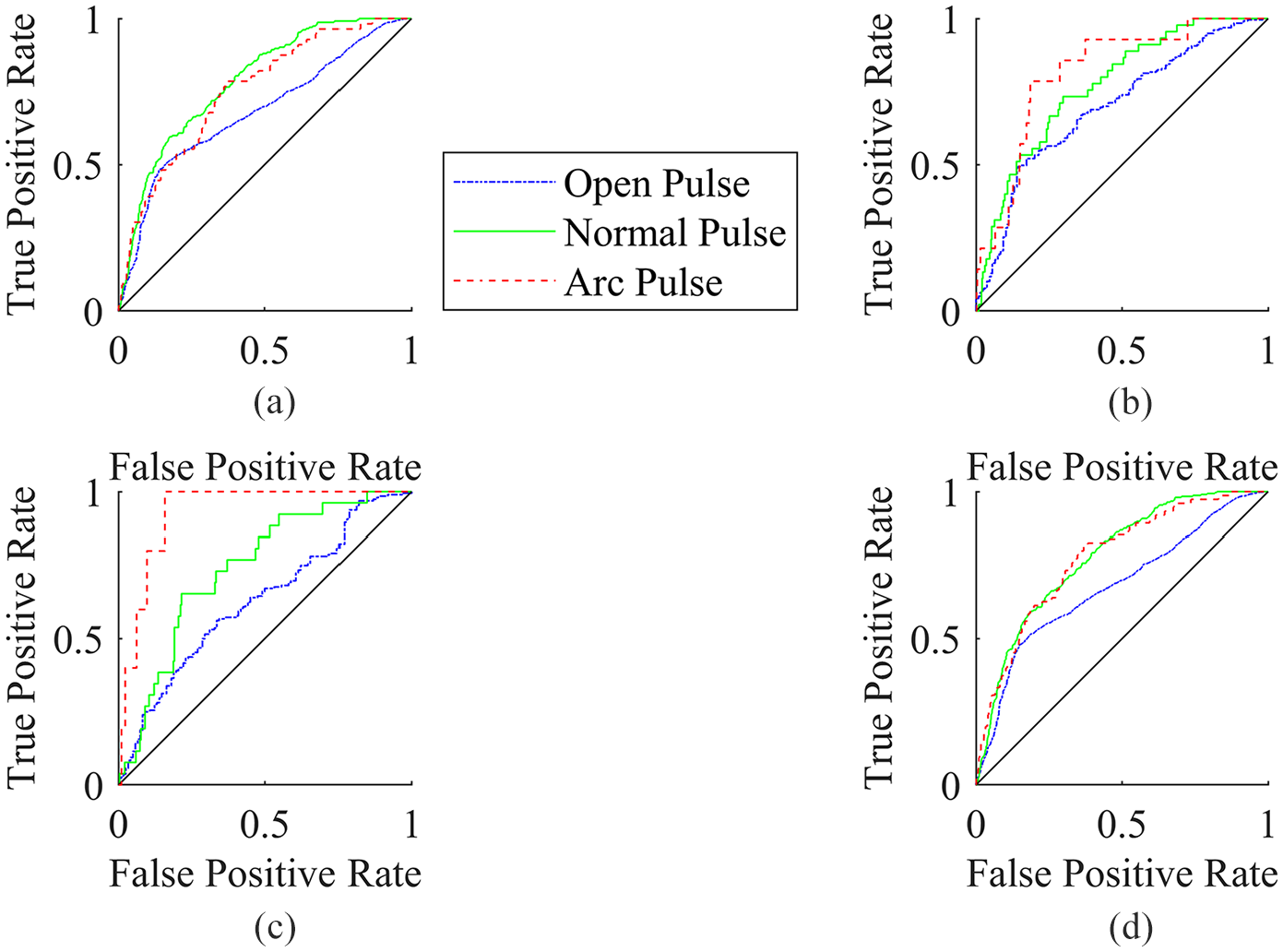
Receiver operating characteristic (ROC) for each class, (a) training ROC, (b) validation ROC, (c) test ROC and (d) all ROC.

As the micro-EDM process is inherently stochastic, the discharge instances are random and often very irregularly distributed for a given data set. Hence, the overall FFBP neural network analysis shows less performance than expected. It requires more adjustments in the network layers, input variables and requires tuning and adjustments of the algorithms.

Scanning electron microscopy on the craters

The scanning electron microscopy (SEM) images of the craters strongly suggest that the material has undergone substantial amount of plastic deformation. As shown in Figure 15, the micro-EDM craters contain the slip bands that indicate that the material has undergone plastic deformation. It clearly shows that the slip bands lie radially to the craters suggesting that the micro-discharges produced mechanical stress on the surface of the workpiece leading to the material deformation in the radially outward direction. Figure 15(a) and (b) shows craters of 32.17 and 24 µm machined with 80 and 120 V, respectively. It was found that the craters were random in size and invariant with the applied voltage with maximum of 50 µm and minimum of 10 µm. The side flow of material is evident which suggest the material has deformed severely. Figure 15(c) shows micro-fractures on the EDM surface. Thus, the SEM images confirm that mechanical deformation (yielding and fracture) has occurred during the crater formation.

Figure 15.

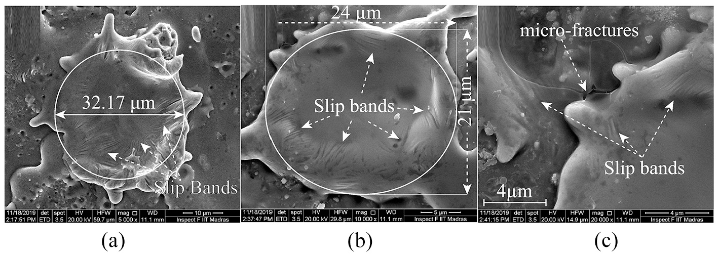
Scanning electron microscope images of the craters: (a) crater at 80 V, (b) crater at 120 V and (c) micro-fracture on the surface.

Conclusion

As the micro-EDM pulses produce discharges of various categories, neither all discharges contribute towards material removal nor do all discharges have the same mechanism of material removal. It is evident that the AE signature for each discharge pulse differs from one pulse class to the other. From the above discussion, the following are concluded.

1. Although melting and vapourisation through thermo-mechanical erosion is the most accepted material-removal process, micro-EDM discharges fit better to the alternative theory of electrostatic force-induced stress yielding. AE burst that occurs during material failure strongly suggests that the material removal happens by mechanical deformation and crack propagation. SEM images show the presence of slip bands and micro-fractures which confirms that the material has undergone severe mechanical deformations.

2. The STFT analysis of the AE signal shows that for a given pulse train of discharge, different categories of pulse produce the different powers of signal over the frequency–time domain. The HHT analysis shows four IMFs that are significant in terms of energy of the signal. AE signal features such as signal strength, signal frequency, phase information, and spectral power are used for monitoring and developing an ANN model.

3. An FFBP neural network model is proposed for monitoring the micro-EDM process with the 10 input vectors constituting of various attributes of the AE signal released during the discharge, and three discharge pulse classes as the output. Ten hidden layers are used to construct the network. The model validation with six validation checks has the cross-entropy of 0.1056 and a convergence gradient of 0.006 at 56 epochs. Although the network performance and the error histogram show a low fitting of the data, the confusion matrix suggests that the overall prediction the pulse categories with the inputs is 66.4%.

The future scope of the work will be to improve the performance neural network model. As the micro-EDM process itself is stochastic in nature, the discharge instances are random and often not evenly distributed which impose a major drawback for training the network. More interesting and significant AE features can be used for pulse-class detection can be explored through further studies. The neural network modelling of micro-EDM is an open-ended research problem.