Sage Journals: Discover world-class research

Abstract

Almost all countries are using railways to transport passengers and freight. Due to heavy load and environmental exposure, these rail sections are prone to damage. Thus, structural health monitoring of the rail section is an essential topic of research to ensure safety and predict the remaining useful life of the track. Consequently, the detection and localisation of damages/cracks in rail section are crucial. It also helps in taking corrective action in time. In this context, the acoustic emission (AE) technique is found to be a powerful non-destructive testing technique which has great potential to localise cracks in rail sections. Actually, the initiation or growth of a damage/crack in a structure emits AE waves, which may be captured using AE sensors mounted on different locations of the structure. The damage itself acts as an AE source. Subsequently, in this study, a novel approach is developed to localise the AE source in a rail section using the artificial neural network (ANN). The ANN model is based on the experimental crack signals captured through a single AE sensor by placing it at different regions of the rail section. For each position of the sensor, cracks are simulated using pencil lead break at different locations along the length and depth of the rail section. It is observed that the developed ANN model predicts the location of the AE source with better accuracy in comparison to the existing localisation methods. The minimum error is found to be less than 1%. Therefore, it can be concluded that the developed ANN model is a suitable option for predicting potential crack locations during real-time monitoring of rail sections.

Keywords

Structural health monitoring rail section acoustic emission technique AE signal artificial neural network non-destructive technique

Introduction

Railways are an important means of transportation in many countries around the world, including India. In recent decades, Indian Railways, the lifeline of the country, has experienced economic and life loss after several derailments, caused mostly by rail iron track failure. The deterioration of the rail iron track may occur due to huge traffic and environmental exposure. Therefore, health monitoring of these rail track networks is the only option to maintain the smooth operation of trains and avoid such risks. Rigorous monitoring of these rail sections using the non-destructive technique (NDT) is necessary to reduce the maintenance cost and evaluate the condition. Damage localisation is one of the main concerns when it comes to monitoring the condition of a structure.¹ However, several conventional NDTs are there to localise damage. Among them, acoustic emission (AE) is the most popular technique, and it has been adopted by many researchers to develop a structural health monitoring system for significant influence on public safety, performance and extending the life of ageing structures.^2–4

Moreover, real-time localisation with accuracy can be done using the same methodology.^5,6 AE method, which is a passive technique, uses elastic stress waves that are released rapidly when a crack initiates and grows.^7,8 This stress wave can be recorded by employing AE sensors over the specimen. AE tomography, damage detection, fracture characterisation, and failure prediction, etc. can be made by analysing the recorded signal.^9–13 This method allows damage to be localised in real time for rail sections without violating the traffic if a sudden failure occurs.¹⁴ These AE sensors are costly, and a large number of sensors are required to detect the damage in the large rail network in India. Here, in this paper, the passive localisation technique using a single AE sensor has been used to make the technique economic.

Since the AE is introduced, several researchers have taken into their research to enhance the accuracy of damage localisation.^13,15 Due to the complex geometry, it is quite difficult to detect damage accurately in the rail section. Each of the different segments of the rail steel section, i.e., top flange (TF), side of TF (STF), web and lower/bottom flange (BF) is considered as a simple plate by several researchers for ease of computation.^16,17 Previously, damage/source localisation in a plate-like structure using the elastic wave propagation rule of AE is examined by Hamstad (1999–2002).^18–20 Also, Hamstad²¹ studied the effect of propagation from different distances and depths in a 25 mm thick steel plate. Thereafter, the source localisation approach using the AE technique has been employed for the diagnosis of the rail sections.²² By installing an AE transducer on the rail top, Bassim²³ demonstrated the AE technique’s vast capabilities in identifying geometric faults on the smooth surface of the wheel periphery. Through creating a test rig, Bruzelius and Mba²⁴ conducted an experiment on the applicability of AE for identifying flaws and surface integrity of iron rail sections. Li et al.²⁵ conducted rail crack monitoring in the field, with complex cracking conditions and operating noise, using Tsallis synchrosqueezed wavelet entropy using the AE approach.

As previously stated, the primary objective of monitoring the rail sections is to locate damage or cracks. Localisation of these cracks is considered the most powerful attribute of the AE technique. In the AE approach, the damage is basically the AE source, which releases AE waves. Thus, damage localisation is similar to the localisation of the AE source. Wavelet transformation (WT) is a powerful signal processing tool, is also available in the literature and is capable to localise damage or cracks in the structure.^26,27 Previously, researchers used WT as a signal processing tool to detect damage or cracks in a sophisticated structure. An experimental investigation for localising cracks using a WT-based localisation technique was done with different propagation distances, types and depths of AE sources by Zhang et al.¹⁶ Kuang et al.²⁸ used the WT-based method for localising cracks on rail heads after noise cancellation. However, in the standard approach and also in the WT-based method, the wave velocity and group velocity of AE waves are required to localise the AE source. Currently, these are obtained using mathematical equations which involve material properties and specimen geometry. But in real-life scenarios, the media through which AE waves travel may not always be homogeneous and isotropic. Moreover, there is a possibility of existing internal defects or discontinuity, etc., inside the material. Therefore, the theoretical wave velocities may often result in erroneous AE source location.

In this context, the ultrasonic pulse velocity (UPV) method, which is another NDT method, can be used to determine wave velocities through the media. UPV is one of the significant NDT methods to detect damage.²⁹ The UPV test is frequently utilised in civil engineering applications, like non-destructive condition assessment of concrete structures such as bridges. This method can provide information about the test object’s surface as well as its inside state.³⁰ In the previous study on UPV, Iyer and Sinha³¹ presented that crack depth in pipes can be detected, and this evaluation can be done using UPV. The ultrasonic wave velocities through the media can be measured by UPV. Therefore, the real-time in situ AE wave velocities may be measured more accurately using UPV than theoretical calculations.

WT-based localisation can be considered an economical technique due to its capability of localisation using a fewer number of sensors.³² For linear localisation, even a single sensor can be applied.³³ But, other than the problem of determination of theoretical and practical group velocities, another concern of WT is the selection of the mother wavelet.³⁴ Signal processing expertise is greatly needed to localise cracks using the WT technique. Using WT, a potential crack in a very small area can be detected because of mode mixing.³⁵ In this context, many researchers have considered artificial neural networks (ANNs) to localise damages or AE sources. The main concept of localisation using ANN is dependable on input and output datasets, weight function, and hidden layers of the algorithm. Previously, few researchers have localised cracks using ANN algorithms.³⁶ Ebrahimkhalou and Salamone³⁷ presented the localisation approach using a deep learning algorithm (autoencoder, softmax layer) by processing the edge reflection of AE waves. Chlada et al.³⁸ showed the localisation of the AE source inside an aircraft structure by making the AE signal’s arrival time profile as input of ANN. Cheng et al.³⁷ presented the localisation approach using ANN for I-shaped girder with an array of sensors after mounting on the web. However, as per the best knowledge of the authors, no work is available in the literature on the AE source localisation in the rail section using ANN. Furthermore, ANN may have the capability of localising damage using a fewer number of sensors, like the WT localisation technique. There is no study in the literature which explored this potential of ANN.

In this study, an effort has been made to develop novel approaches for localising AE sources more accurately in different longitudinal distances and transverse locations in the rail section. The study describes two different approaches to localising AE sources more accurately than the existing WT-based method. Application of the AE technique in localising damage/AE source in real time requires AE wave velocity inside the given specimen and time-of-arrival (TOA) of the AE wave in the sensor(s). In general, velocity is computed theoretically based on the standard material properties as provided by the manufacturer/supplier. TOA is found out from the WT diagram of the captured sensor signal. In reality, the theoretical velocity may not represent the actual velocity in rail as the rail sections are subjected to adverse loading and weathering conditions. Therefore, measurement of the true velocity in the field is expected to yield better localisation of the AE source. Accordingly, in this paper, as a first attempt to develop a realistic and accurate AE source localisation methodology, in situ velocity measurement is made with the help of UPV. Consequently, the obtained results for localisation are better (<9%) than the conventional WT method. As a further effort to make the AE source localisation methodology even more effective and accurate, the authors have also tried to present an ANN model for source localisation using AE sensor data. This model is found to predict the source location with more accuracy than the conventional WT method as well as the modified WT method, as proposed earlier in this study. Therefore, this study makes a novel contribution in regard to localisation through an ANN-based modelling approach, which is more effective and simpler. Also, it can be stated that only AE sensor data, and no data regarding material property, are required to find out the AE source distance in the developed ANN-based approach. In this study, all three methods have been carried out in the laboratory on the rail section of 1.9 m length. In this paper, pencil lead break (PLB) or Hsu-Nielsen source is used to simulate artificial damage, which is synonymous with actual AE source. In this case, the brake signal of the pencil lead travels through the rail section. A single wide-band (WD) AE sensor is placed at each individual component of the rail section to capture signals emitted from the AE source. The AGU-Vallen³⁹ WT tool is used to process the AE signals. MATLAB is used to develop an ANN algorithm using fundamental characteristics as input for the localisation of AE source in the rail section. Through the experimental investigation, it is observed that the AE sources can be localised for unknown wave velocity of materials using the WT technique with limitations, and the simulated AE source has been localised perfectly using the developed ANN algorithm.

Methodology

WT-based localisation

WT-based localisation using theoretical velocity

WT is a powerful tool to detect damages with accuracy by analysing the obtained AE signal in the rail section. Therefore, many researchers have taken the help of this standard and reliable technique to detect the AE source accurately. In this mentioned approach, the distance between the AE sensor and the AE source is calculated using the TOA of the fundamental Lamb modes using WT.

The WT algorithm is used in this experiment for analysing the characteristics of AE signals for the localisation of AE signals. Since the AE signal consists of more than one wave mode, which is called Lamb wave mode, the WT algorithm is useful for solving this process.⁴⁰ The function f(t) of time t of WT is defined as⁴¹:

W_{ψ}^{f} (a, b) = \int_{- \infty}^{+ \infty} f (t) ψ_{a, b}^{*} (t) d t

(1)

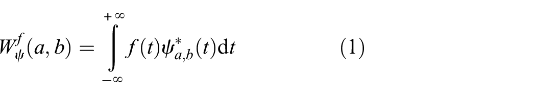
where $ψ_{a, b} (t) = (ψ ((t - a) / b) / \sqrt{b})$ , and $ψ^{*} (t)$ is the complex conjugate of the mother function ψ(t), a and b are the translation and scale parameters, respectively.

Preparation of group velocity curves:

The group velocity curve on the TF, STF, web and the BF of the rail section is calculated using the surface wave.⁴¹ However, the group velocity curve has to superimpose over the WT diagram of the obtained AE signal to understand the features of the AE signal, which are shown in Equations (2)–(4):

Symmetric modes : \frac{\tan (qh)}{\tan (ph)} = - \frac{4 k^{2} pq}{{(k^{2} - q^{2})}^{2}}

(2)

Antisymmetric modes : \frac{\tan (qh)}{\tan (ph)} = - \frac{{(k^{2} - q^{2})}^{2}}{4 k^{2} pq}

(3)

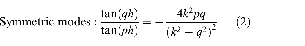
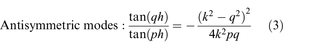
where

p^{2} = \frac{w^{2}}{c_{l}^{2}} - k^{2}, q^{2} = \frac{w^{2}}{c_{t}^{2}} - k^{2}

(4)

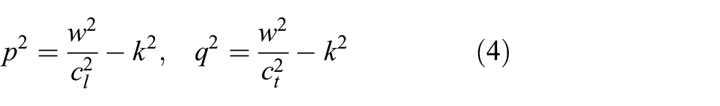
In the equations, ‘h’ denotes half of the plate thickness, ‘ω’ represents the angular frequency, ‘k’ denotes the wavenumber, ‘c_l’ represents longitudinal wave velocity and ‘c_t’ is shear wave velocity. Then, phase velocity: c_p = ω/k and group velocity: ‘c_g = ‘dω/dk’” has been calculated.

Localisation using WT and UPV

Localising the AE source using WT and plotting the group velocity curve is necessary to determine the TOA of different Lamb modes. The longitudinal and shear velocity of AE waves in the media is the main concern in producing the group velocity curve. In practical life, the velocity of such ultrasonic waves changes due to the presence of internal faults or discontinuity. Therefore, UPV testing is done to detect this wave velocity through the rail section (Figure 1).

Figure 1.

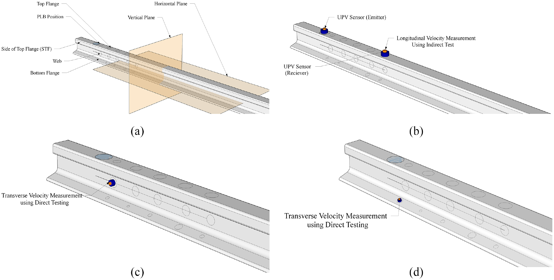
(a) Details of the rail section and longitudinal direction and transverse direction, (b) direct test for the longitudinal velocity at TF, (c) indirect test for the transverse velocity at the web and (d) indirect test for the transverse velocity at BF.

The UPV method uses an electro-acoustical transducer to generate ultrasonic pulses. There is a receiving transducer and emitting transducer in the UPV instrument. When the pulse is induced into the specimen, it reflects multiple times at the boundaries of distinct material phases within the specimen. The resulting stress waves include longitudinal (compressional), shear (transverse) and surface (Rayleigh) waves, forming a complex system. The receiving transducer detects the start of the fastest transverse and longitudinal waves.⁴²

The pulse velocity method is a convenient tool for analysing the specimen since the velocity of the pulses is almost independent of the geometry of the material through which they pass and solely depends on its elastic characteristics (Figure 1).

The ultrasonic pulse is generated by a transducer that is in contact with one surface of the specimen under test in this test procedure. The pulse of vibrations is transformed into an electrical signal by the second transducer maintained in touch with the other surface of the concrete member after travelling a specified path length L in the specimen, and the pulse’s transit time (T) can be quantified using an electronic timing circuit. The pulse velocity (V) for the direct and indirect tests is calculated as follows²⁹:

V = L / T

ANN-based localisation

A novel source localisation approach is presented in this paper using ANN. ANN is a powerful tool that can predict the location of damage by analysing provided datasets for training. Figure 2 depicts the novel approach to detecting simulated AE sources in the rail section. As the rail section is in undamaged condition, PLB has done to generate AE sources which is synonymous with the actual crack. In this paper, the discussed AE source is localised by developing ANN where fundamental features of the AE signal is considered as input. Therefore, obtaining good-quality signals is the main concern for this technique. These fundamental features of the AE signal are shown in Figure 3 (rise time, duration, energy, peak frequency, count, root mean square) taken to train the ANN model. In this testing procedure, these features or parameters are collected in laboratory conditions. However, these parameters are unstable in the noisy environment. Signal processing with noise cancellation technique is required for in-field environment.¹⁰ For the convenience of the experiment, these features are separated into four clusters. These clusters are mentioned in Table 1. After that, the ANN model is prepared in MATLAB. The ANN model uses 4 hidden layers and 20 neurons consisting of each layer. Figure 4 depicts the architecture of the ANN model developed in MATLAB. Table 2 depicts the orientation of the dataset for input, training and testing purpose.

Figure 2.

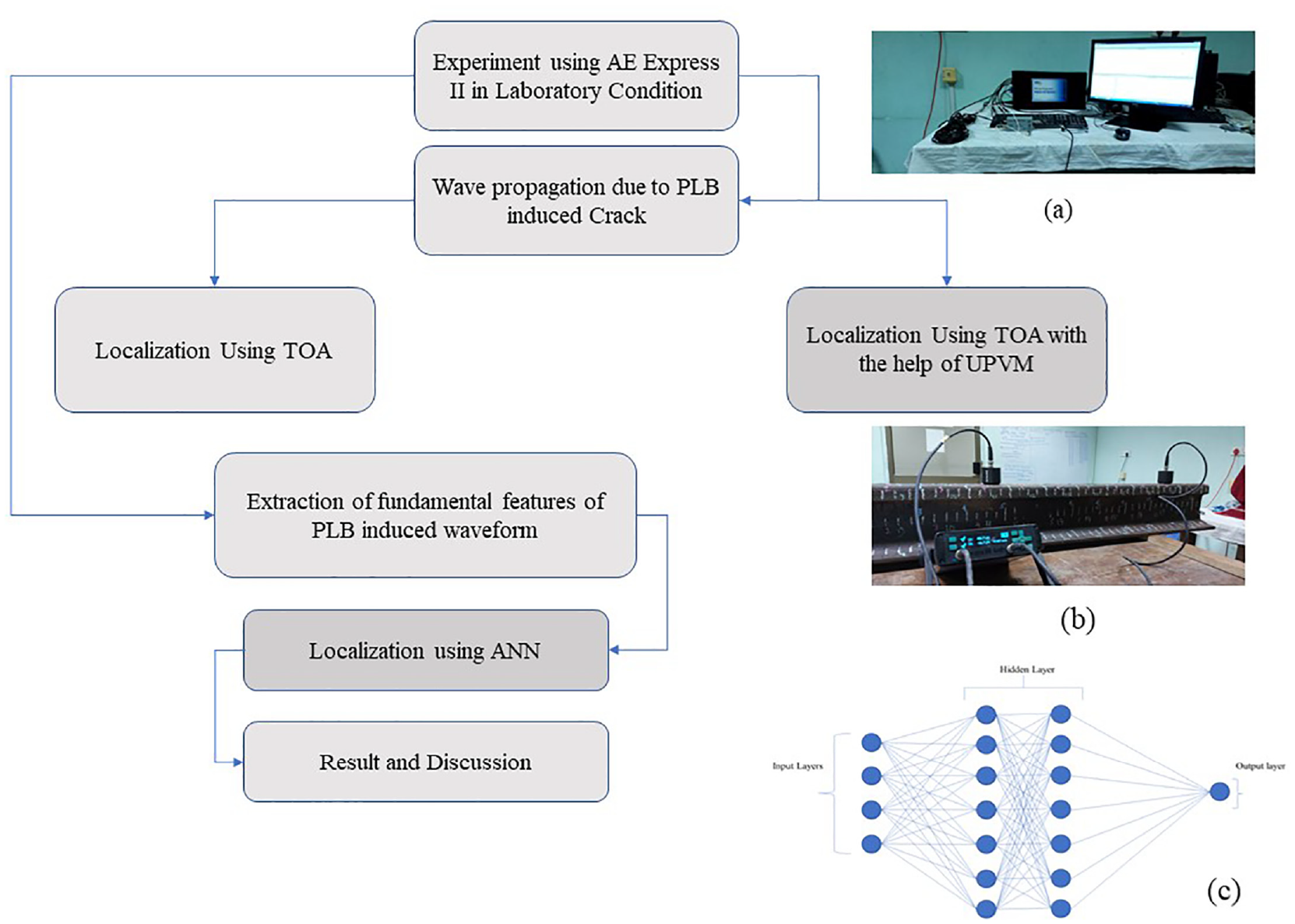
Flowchart of the approach: (a) AE Express II Instrument, (b) Finding Velocity with UPV, (c) Graphical Representation of ANN model.

Figure 3.

Fundamental features of AE wave.

Table 1.

Clusters made for ANN.

Cluster	Arrangements of fundamental properties of signal
C1	Rise time, energy, amplitude, peak frequency
C2	Rise time, counts, energy, duration
C3	Rise time, duration, counts, RMS
C4	RMS, rise time, counts, peak frequency, amplitude

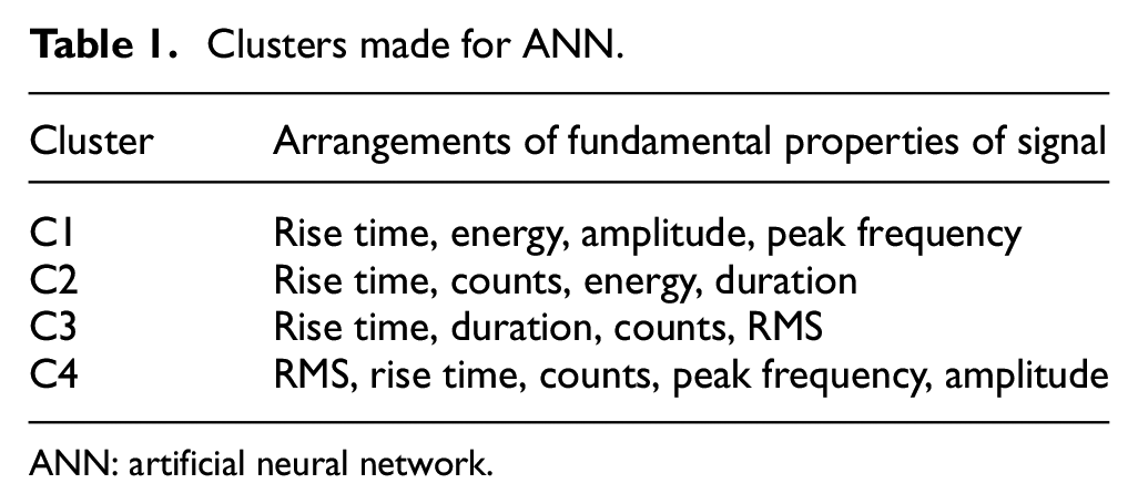
ANN: artificial neural network.

Figure 4.

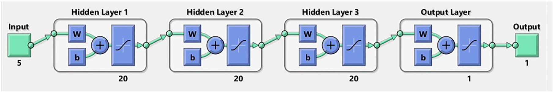
Architecture of the developed ANN model.

Table 2.

ANN data structure.

ANNCluster	Data structure		Model parameter
	Input size	Training/test samples	Trainable
C1	1200X4	800/350	4800
C2	1200X4	800/350	4800
C3	1200X4	800/350	4800
C4	1200X4	800/350	4800

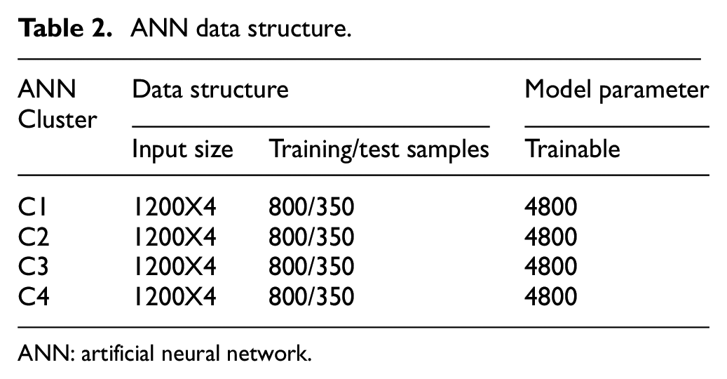
ANN: artificial neural network.

Experimental setup

To localise the damage in the rail section with the adopted methodology, the following setup is done. Figure 4 depicts the experimental setup for testing in the rail section. The experiment is carried out on a 1.9 m rail section provided by Indian Railways. The data acquisition system for AE monitoring is procured from Physical Acoustic Corporation (PAC). PLB is taken to simulate the AE source in the media. A differential type (WD) AE sensor or transducer, procured from PAC, is utilised as a receiver of AE signal to capture the simulated AE wave generated from different AE sources to sensor distances. Figures 5(b) and 6(b) are the representation of the placement of the AE sensors (WD) over the rail section.

Figure 5.

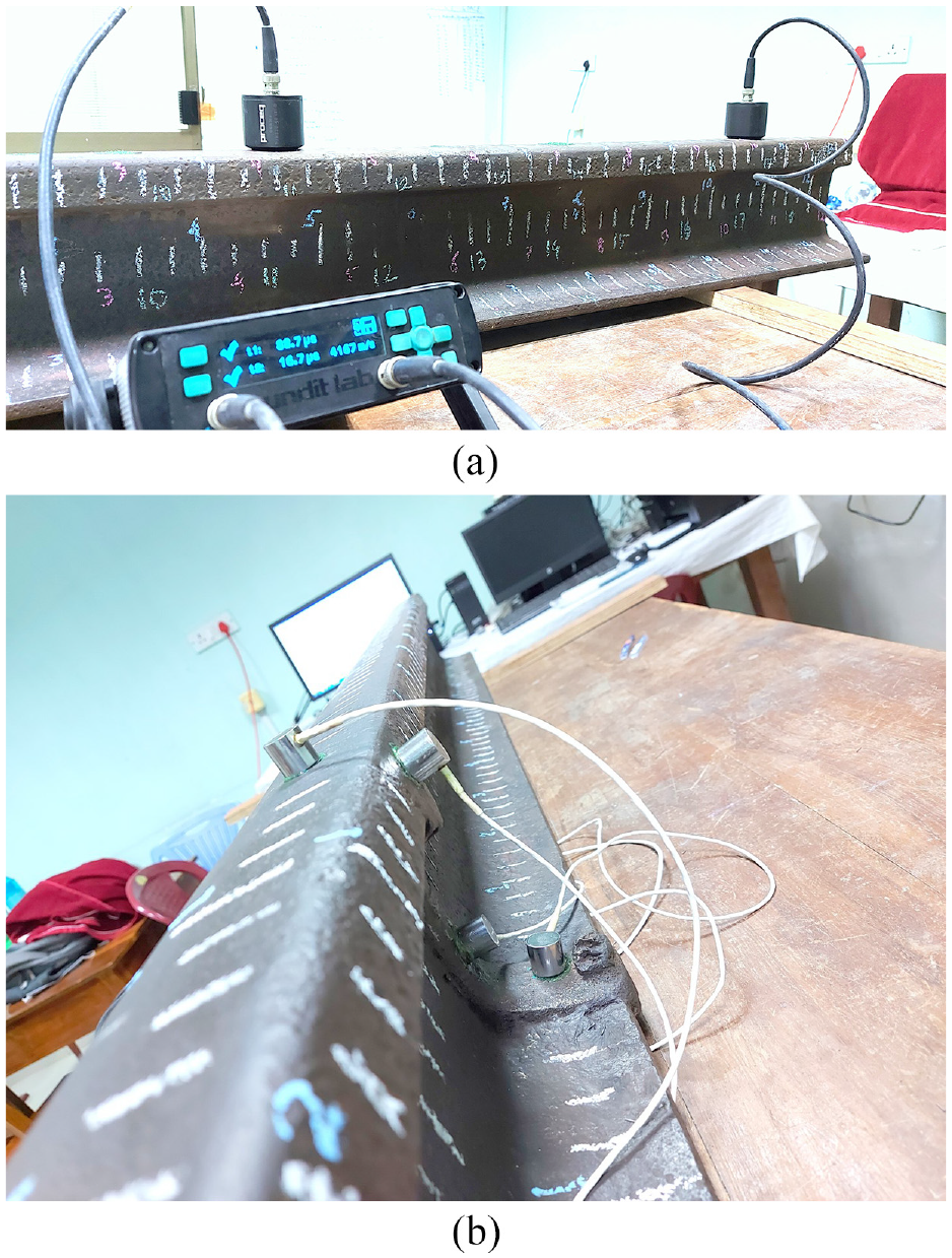
The experimental setup and placement of sensor for rail testing: (a) AE instrument and (b) rail section.

Figure 6.

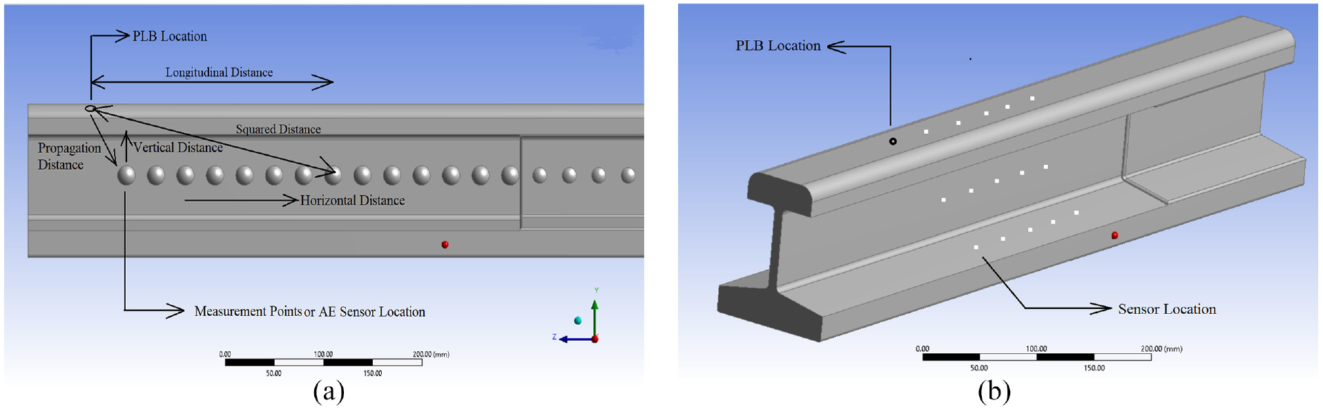
Representation of the side view of the rail and PLB and AE sensor location: (a) measurement of the source distances and (b) sensor and crack location on the rail section.

The bulk longitudinal and shear velocity of the rail section is 5900 and 3100 m/s, respectively, and were used to produce theoretical group velocity curves. An UPV tester manufactured by PUNDIT LAB is used to get the actual velocities of the rail track.

Measurement positions on the TF, web and BF of the rail section are depicted in Figure 6(a). For testing reasons, multiple measurement points in the mentioned segment in the rail section were considered. The AE receiver was mounted on flat places such as the head to TF, the web of the rail section and the flat area of the BF. The AE receiver is installed on a web that is 70 mm below the rail section’s TF. With 50 mm intervals, measurement positions have reached up to 1200 mm. Acquiring a consistent and homogeneous actual simulated acoustic source is fairly difficult due to complex geometry of the rail section. PLB is an established method to simulate AE signals artificially. Therefore, in this paper, PLB is done over the TF, and the simulated AE signal is captured from different depths and segments of the rail section. The frequency obtained from the recorded AE signal lies in between 100 and 300 KHz.

All of the data in this research were collected using the AE acquisition system (AE Win 8) at a sampling frequency of 1 MHz. All data were evaluated during a time span of 0–200 s. The surface equation and WT algorithm were utilised to detect and evaluate the acquired data using the ‘AGU-Vallen WT’ tool.²¹

The group velocity curve is crucial for determining the primary modes of AE wave propagation. As a result, UPV is used to calculate the P and S wave velocities. The longitudinal and transverse wave velocities are measured using indirect and direct tests.

Experimental studies

In the above-mentioned approach, the group velocity curve is calculated using both theoretical and experimental results. To superimpose the curve on the WT diagram, the group velocity curve was transformed to a timescale using the previously estimated propagation through the rail segment. The varied propagation distances were determined by square rooting the sum of the AE source’s squared distances Figure 6(a). The BF of the rail section has a complex shape and a non-uniform thickness in the vertical direction. The average thickness of the TF and the web is taken at 40 and 18 mm, respectively, to compute the group velocity curve.

In the WT diagram with the group velocity curve, different colours denote distinct modes. Figure 7 depicts information from the rail section’s group velocity curve at TF, web and BF. The validation of the surface wave, that is, the Lamb wave equation, has been the emphasis of this paper to determine the depth and propagation lengths of a simulated AE source. The WT of the AE signal is shown in Figures 8 and 9, and it is corroborated by superimposing the group velocity curves of different depths of the rail section.

Figure 7.

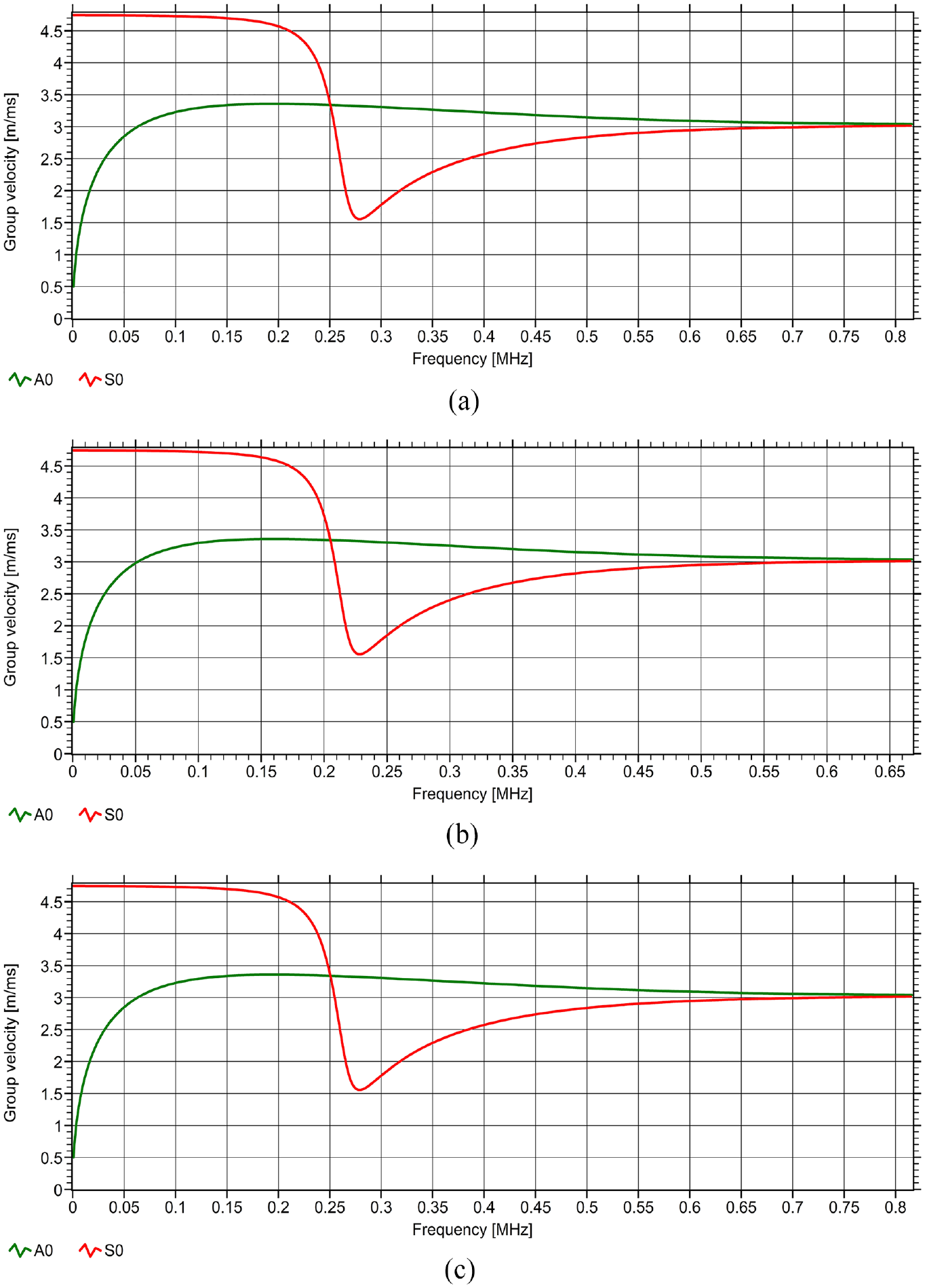
Practically obtained group velocity curve using UPV from different segment of rail section: (a) TF, (b) web and (c) BF.

Figure 8.

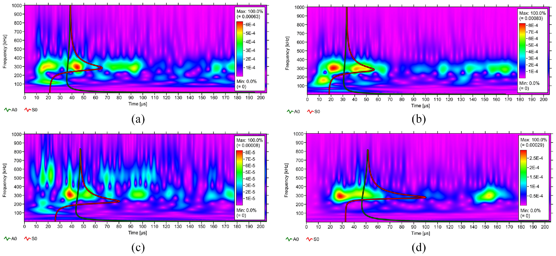
WT diagram and theoretically calculated group velocity curve for (a) when sensor mounted on rail head, (b) STF, (c) web and (d) BF.

Figure 9.

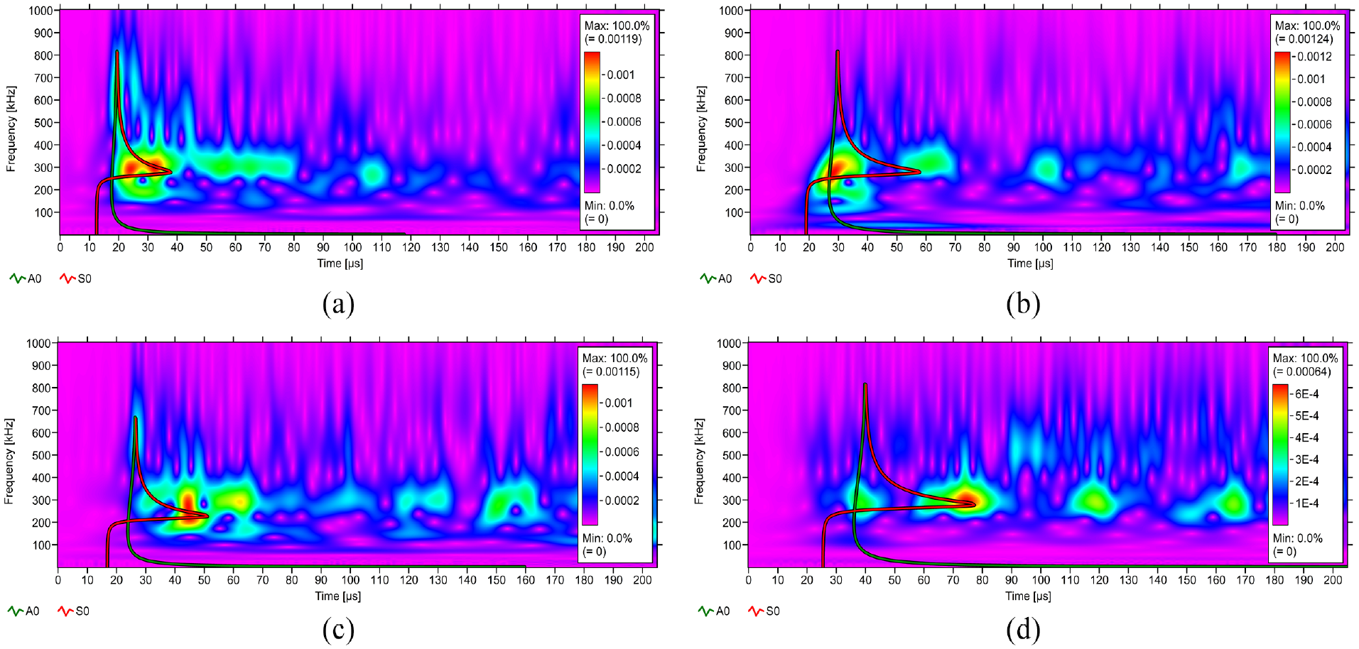
WT diagram after plotting group velocity curve of PLB-induced AE wave when group velocity is calculated using UPV: (a) sensor mounted on rail head, (b) STF, (c) web and (d) BF.

These signals, which were received from simulated AE sources at various distances and depths from the observed sites, were examined. The WT diagram shows a high energy concentration zone (red zone). For localisation purposes, the group velocity curves are plotted and superimposed over the WT diagram of the captured signal from TF, web and BF to match the high energy concentration zone. However, it is observed that the response from the TF is better than web and BF. There was also a comparison of theoretical and experimental wave velocity. The high energy concentration region and related peak frequency of WT have been found for the collected AE signal. The matching Lamb modes and distance from the AE source were then determined using the group velocity curve. By multiplying the group velocity corresponding to the peak WT coefficient frequency and time, the defect/AE source/PLB distance may now be calculated. In this paper, Lamb modes (S₀ and A₀) have been considered regarding the localisation of AE sources. Tables 3 and 4 summarise the findings.

Table 3.

Theoretical P wave and S wave velocity from AGU-Vallen tool.

Location	Longitudinal wavevelocity (m/s)	Shear wavevelocity (m/s)
TF	5950	3240
Web	5950	3240
BF	5950	3240

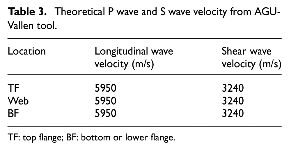
TF: top flange; BF: bottom or lower flange.

Table 4.

P wave and S wave velocity using UPV.

Area of test	Indirect/longitudinal wave velocity		Direct/shear wave velocity
Area of test	Velocity (m/s)	Avg. velocity (m/s)	Velocity (m/s)	Avg. velocity (m/s)
TF	4975	4778.66667	3521	3571
	4125		3650
	5236		3542
Web	4895	4721.66667	3478	3565.333333
	4158		3654
	5112		3564
BF	4921	4803	3145	3527.666667
	4752		3556
	4736		3882

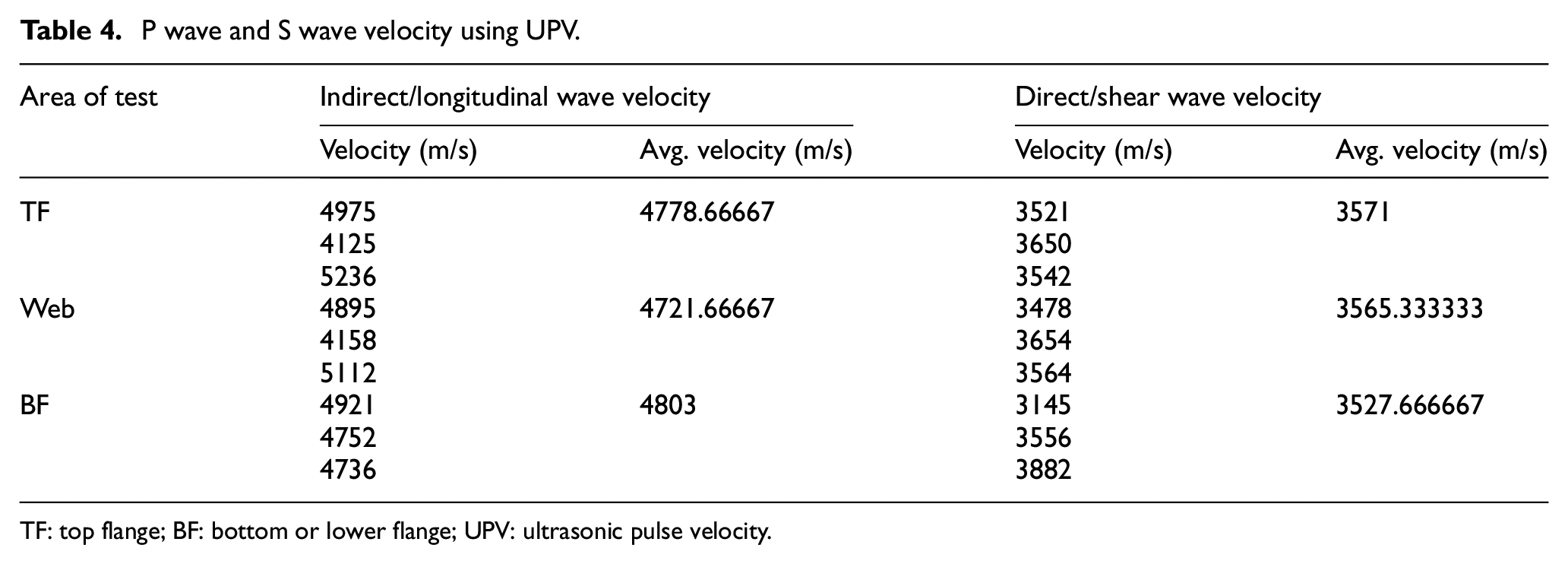
TF: top flange; BF: bottom or lower flange; UPV: ultrasonic pulse velocity.

Result and discussion

WT-based localisation with theoretical velocities

While PLB is performed on the railhead or TF, the AE sensor is moved at 10 mm intervals up to 1200 mm to gather strong signals produced by the simulated AE source. Following that, the WT of the recorded signals is performed to precisely locate AE sources.

For the railhead, it matches well with the theoretically calculated fundamental Lamb modes, but in the rail BF and web, these modes are not matching. It is observed that the theoretically calculated group velocity is not matching when superimposed over the WT diagram of obtained AE signal from the BF of the rail section. However, the theoretically calculated group velocity is fairly matching with the WT diagram of the AE signal obtained from TF, STF and the BF segment of the rail section.

The WT diagrams of the recorded AE signal in the rail section, computed theoretically and experimentally, are shown in Figures 8 and 9. It is observed that the energy concentration consistent change throughout the rail segment when signal is captured from TF, STF, web and BF. The energy concentration regions in the WT correspond to the group velocity curve of the rail web, with TF and STF regions showing a uniform difference when plotted as a reference. The group velocity curve was generated by considering the TF of the rail section as a thick plate. However, the wave velocity for the web and base of the rail section decreases, and the group velocity curves are validated and matched well using experimental values instead of theoretical values.

The WT diagram of the recorded AE signal from different segments of the rail section is shown in Figure 8. The energy concentration region on the WT diagram of obtained AE signal from TF, STF and web are slightly matching well with the corresponding regions’ group velocity curves. But the group velocity curve is not perfectly fitted over the WT diagram of the obtained signal from BF.

The group velocity curve from the UPV results is now tried to match the WT diagram of obtained AE signal from different segments of the rail section. Figure 9 shows the same group velocity curve made by the UPV results matches well. The comparison of the results obtained from both cases is shown in Tables 5 –7. It is clear from Figure 9 that the group velocity curve made by in situ results obtained from UPV is giving satisfactory results. But it is observed that the localisation of the AE sources using the signal processing approach is valid up to a certain distance. Due to mode mixing, this signal processing approach is not actually helpful when the AE propagation distance is too long.

Table 5.

Localisation of AE sources at rail head and error % in localisation.

Distance (mm)	Localisation using			Error (%)
Distance (mm)	WT (Theo) or TOA	WT (Exp) + UPV	ANN	WT (Theo) or TOA	WT (Exp) + UPV	ANN
50	44.149	49.557	50.112	13.254	0.895	0.223
100	99.254	101.222	100.540	0.751	1.207	0.537
150	151.413	149.245	150.416	0.933	0.506	0.277
200	204.179	198.416	199.478	2.046	0.798	0.262
250	247.566	249.556	250.004	0.983	0.178	0.002
300	294.255	301.413	299.875	1.952	0.469	0.042
350	348.622	349.741	350.115	0.395	0.074	0.033
400	394.756	399.485	400.214	1.328	0.129	0.053
450	461.399	449.402	450.373	2.470	0.133	0.083
500	503.126	499.318	500.074	0.621	0.136	0.015
550	553.855	549.235	550.634	0.696	0.139	0.115
600	604.530	599.152	600.227	0.749	0.142	0.038
650	655.652	649.069	650.041	0.862	0.144	0.006
700	705.921	698.985	700.375	0.839	0.145	0.054
750	756.676	748.902	750.731	0.882	0.147	0.097
800	807.331	798.819	800.432	0.908	0.148	0.054
850	858.022	848.735	850.173	0.935	0.149	0.020
900	908.745	898.652	900.647	0.962	0.150	0.072
950	959.425	948.569	950.742	0.982	0.151	0.078
1000	1010.642	998.485	1000.495	1.053	0.152	0.049
1050	1060.993	1048.402	1050.114	1.036	0.152	0.011
1100	1111.522	1098.319	1100.012	1.037	0.153	0.001
1150	1162.667	1148.235	1150.147	1.089	0.154	0.013
1200	1212.927	1198.152	1200.621	1.066	0.154	0.052

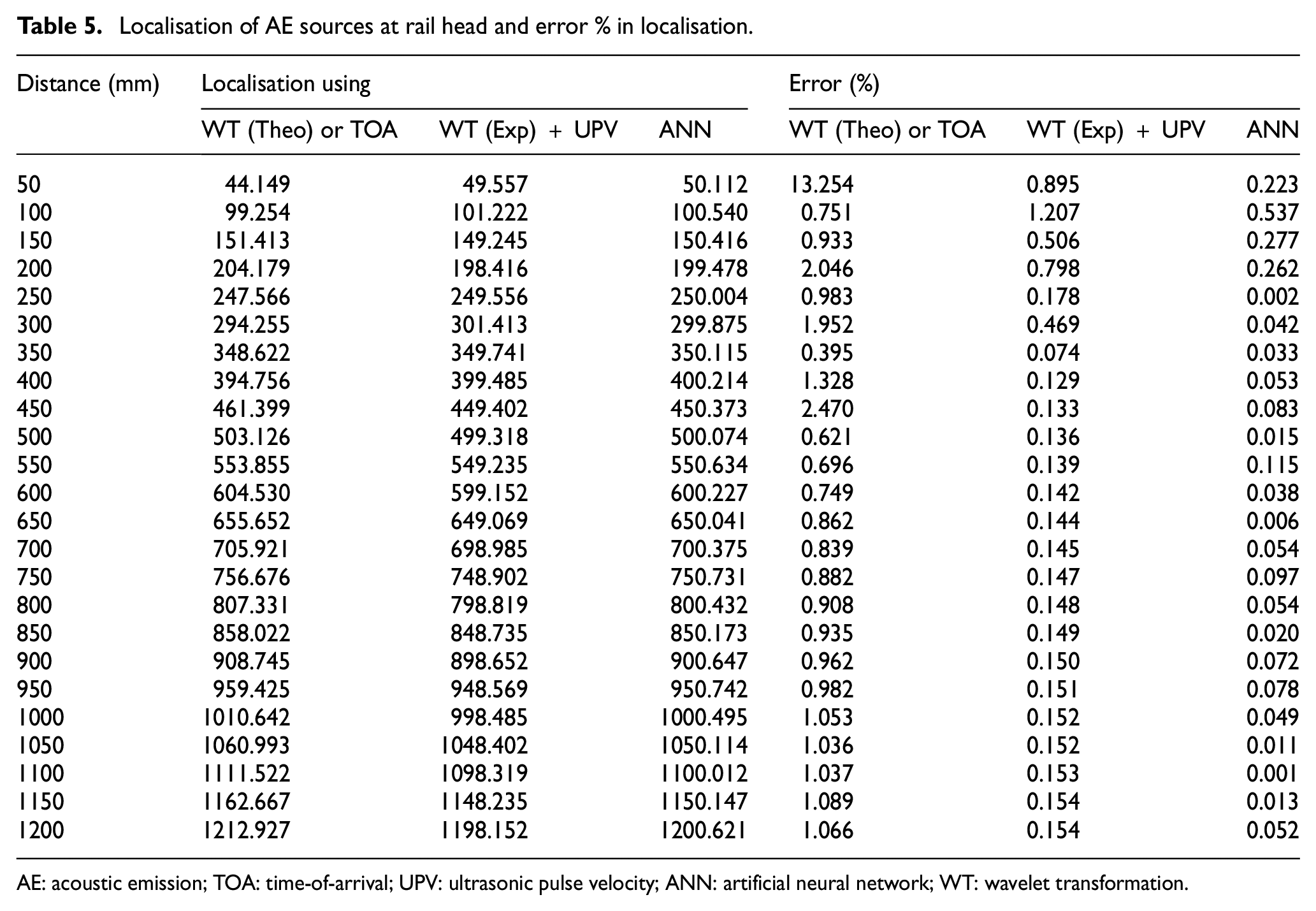
AE: acoustic emission; TOA: time-of-arrival; UPV: ultrasonic pulse velocity; ANN: artificial neural network; WT: wavelet transformation.

Table 6.

Localisation of AE sources at rail web and error % in localisation.

Distance (mm)		Localisation using			Error (%)
Actual	Squared	TOA	TOA + UPV	ANN	TOA	TOA + UPV	ANN
50	86.023	87.147	86.447	86.230	1.289	0.490	0.240
100	122.066	124.983	122.456	122.057	2.334	0.319	0.007
150	165.529	167.124	164.547	165.522	0.954	0.597	0.005
200	211.896	208.447	214.266	211.880	1.655	1.106	0.008
250	259.615	247.156	258.021	259.636	5.041	0.618	0.008
300	308.058	307.941	308.192	308.055	0.038	0.043	0.001
350	356.931	341.648	355.153	356.925	4.474	0.501	0.002
400	406.079	384.842	397.164	406.075	5.518	2.245	0.001
450	455.412	428.037	442.559	455.425	6.396	2.904	0.003
500	504.876	471.231	487.954	504.845	7.140	3.468	0.006
550	554.437	514.426	533.349	554.218	7.778	3.954	0.039
600	604.070	557.621	578.744	604.086	8.330	4.376	0.003
650	653.758	600.815	624.139	653.165	8.812	4.746	0.091
700	703.491	644.010	669.535	703.563	9.236	5.072	0.010
750	753.260	687.205	714.930	753.179	9.612	5.361	0.011
800	803.057	730.399	760.325	803.045	9.948	5.620	0.001
850	852.877	773.594	805.720	852.350	10.249	5.853	0.062
900	902.718	816.788	851.115	902.621	10.520	6.063	0.011
950	952.575	859.983	896.510	952.156	10.767	6.254	0.044
1000	1002.447	903.178	941.905	1003.015	10.991	6.428	0.057
1050	1052.331	946.372	987.301	1053.276	11.196	6.587	0.090
1100	1102.225	989.567	1032.696	1103.554	11.385	6.733	0.120
1150	1152.128	1032.762	1078.091	1154.566	11.558	6.867	0.211
1200	1202.040	1075.956	1123.486	1205.564	11.718	6.992	0.292

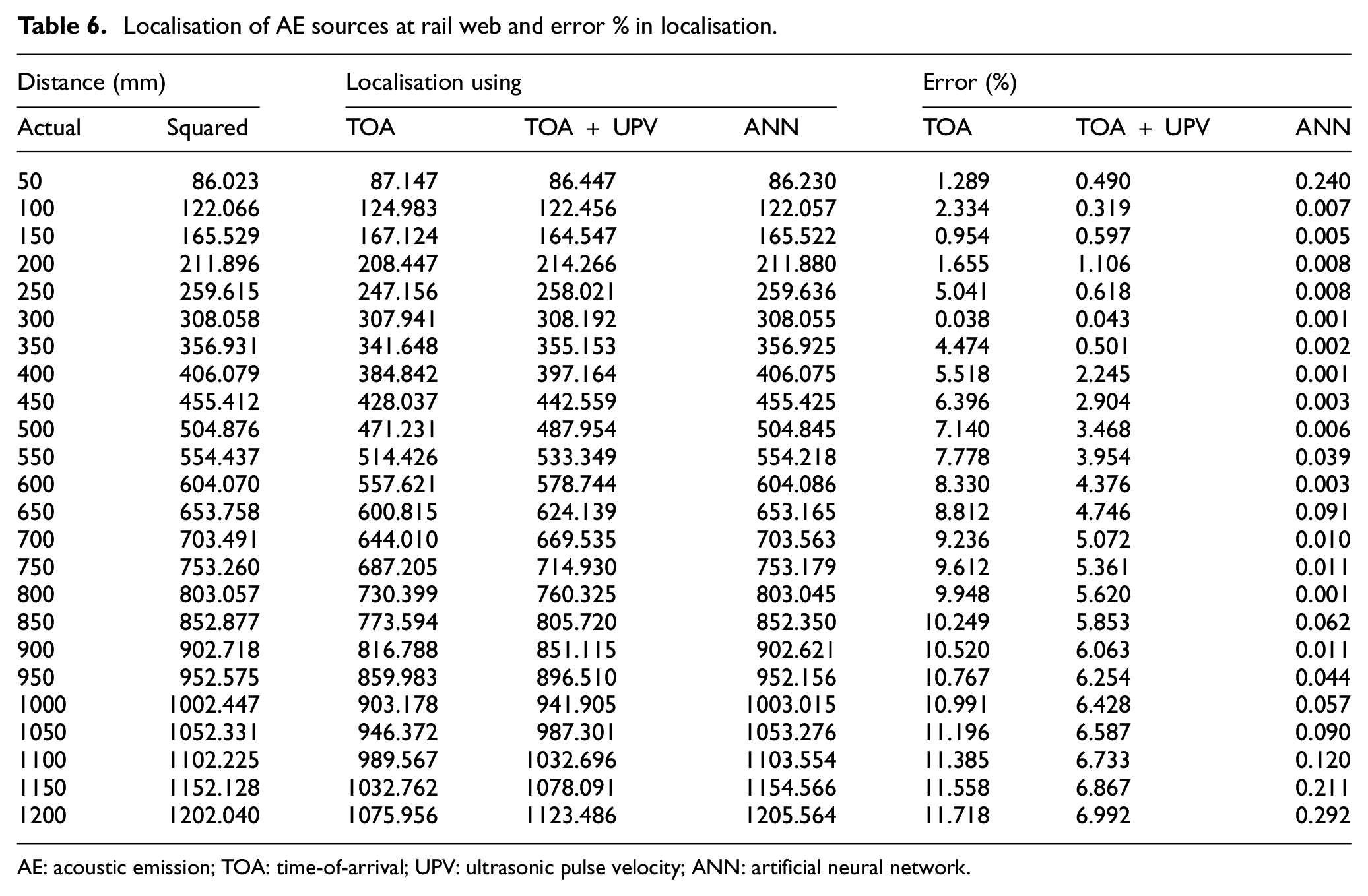
AE: acoustic emission; TOA: time-of-arrival; UPV: ultrasonic pulse velocity; ANN: artificial neural network.

Table 7.

Localisation of AE sources at Rail BF and Error % in localisation.

Distance (mm)		Localisation using			Error (%)
Actual	Squared	TOA	TOA + UPV	ANN	TOA	TOA + UPV	ANN
50	177.200	160.453	173.512	177.432	10.438	2.126	0.130
100	197.231	186.166	198.115	197.240	5.944	0.446	0.005
150	226.716	223.225	224.007	226.462	1.564	1.209	0.112
200	262.488	264.113	260.997	262.658	0.615	0.571	0.065
250	302.324	298.345	300.731	302.556	1.334	0.530	0.077
300	344.819	342.696	343.418	344.875	0.619	0.408	0.016
350	389.102	387.081	390.653	389.473	0.522	0.397	0.095
400	434.626	432.167	434.013	434.615	0.569	0.141	0.003
450	481.041	480.253	480.974	481.521	0.164	0.014	0.100
500	528.110	521.467	527.156	528.002	1.274	0.181	0.020
550	575.674	573.161	574.257	575.615	0.438	0.247	0.010
600	623.618	618.491	622.774	623.563	0.829	0.136	0.009
650	671.863	669.436	670.841	671.976	0.363	0.152	0.017
700	720.347	717.259	719.489	721.564	0.431	0.119	0.169
750	769.025	764.339	768.115	770.341	0.613	0.119	0.171
800	817.863	807.419	816.740	817.873	1.293	0.137	0.001
850	866.833	856.500	876.366	866.228	1.207	1.088	0.070
900	915.915	921.580	918.991	915.796	0.615	0.335	0.013
950	965.091	961.660	964.616	965.155	0.357	0.049	0.007
1000	1014.347	1015.740	1013.242	1013.597	0.137	0.109	0.074
1050	1063.673	1057.821	1065.867	1064.593	0.553	0.206	0.086
1100	1113.059	1124.901	1117.493	1113.743	1.053	0.397	0.061
1150	1162.497	1168.981	1061.118	1167.326	0.555	9.554	0.414
1200	1211.982	1219.062	1212.744	1212.559	0.581	0.063	0.048

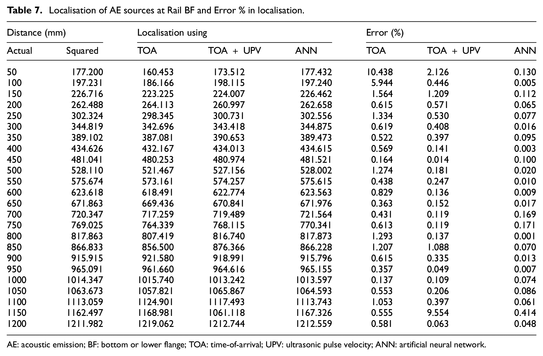
AE: acoustic emission; BF: bottom or lower flange; TOA: time-of-arrival; UPV: ultrasonic pulse velocity; ANN: artificial neural network.

ANN-based localisation

The results show that the group velocity curve for the rail TF and web matches approximately with the WT diagram for the same segment of the rail section, but for the bottom or the lower flange, it is not matching well. The group velocity curve matches well with the WT diagram up to a certain distance. This research deals with the localisation of AE sources using signal processing and using the ANN approach. Due to the complex geometry of the rail section, signal processing approach is critical. Propagation of ultrasonic wave behaves different and random in the rail section. Therefore, signal distorted when travel and reflects back. With the signal processing approach, the localisation of AE source is difficult. According to the signal capturing procedure and geometry of the specimen rectification and modification are severely needed. But ANN works with the data of acquired signal from any portion of the rail section. In a complex geometry like rail, ANN is the suitable option for localising AE sources. In this paper, the energy concentration regions from the WT diagram and fundamental features of the AE signal are taken to localise the AE sources. The fundamental parameters or features are analysed with the ANN model about their influence on the AE signal.

The ANN model was prepared in MATLAB. To precisely detect damage locations, four clusters are prepared using data-driven parameters. The developed ANN model uses different types of weight functions in the input layer, and weight functions are introduced in all four clusters to assess the model’s performance. The developed ANN model’s performance is checked and validated using the trial-and-error method. Figure 10 shows that cluster four can predict the appropriate result as the R value is closer to 1. The number of neurons in the ANN’s hidden layer influences the mean square error (MSE) and R. The R value ranges from 0 to 1 and reflects the relationship between output and targets. In this investigation, the model uses five input layers and four hidden layers, with each hidden layer consisting of twenty neurons. The ANN model uses MSE to obtain an output value as close to the target value as possible. Feed-forward backpropagation is introduced in the model to achieve the target value, and the model is stopped after 750 iterations. On average, the ANN model takes 15.5 min to complete each localisation process. The configuration of the computation system in which the developed ANN model runs has an intel i7-8Gen processor with 4core, eight logical processors and 8GB DDR4 RAM.

Figure 10.

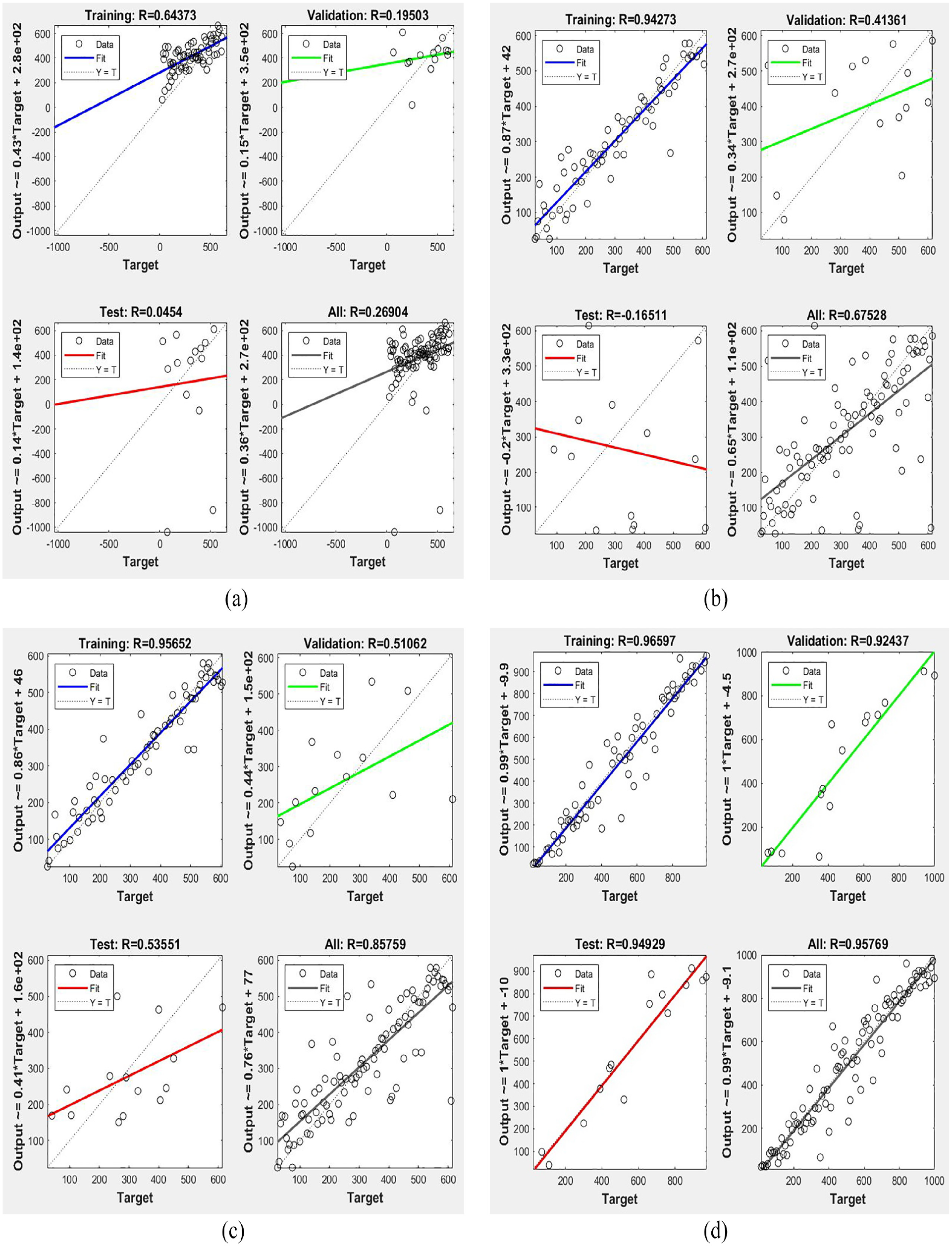
Performance of developed ANN model represents (a) cluster 1, (b) cluster 2, (c) cluster 3 and (d) cluster 4.

An actual size rail track has been procured from Indian Railways for monitoring purposes using the AE technique. AE source localisation using the developed ANN model is finally compared with the WT localisation technique to check the efficacy.

From Figure 11, it can be detected that the AE source can be localised from any portion of the rail section. In this study, the training process with the developed ANN model is done for PLB-induced signals up to 500 mm. There, a new set of simulated AE signals due to PLB is recorded for 1200 mm. Though the existing localisation technique gives almost the correct distance of the AE source, it is a lengthy and complicated process. More accurate localisation is done using the developed ANN model, which is based on the fundamental characteristics of the AE signal in the media. The proposed methodology is a comparatively less complicated and reliable technique to detect AE sources up to a long distance.

Figure 11.

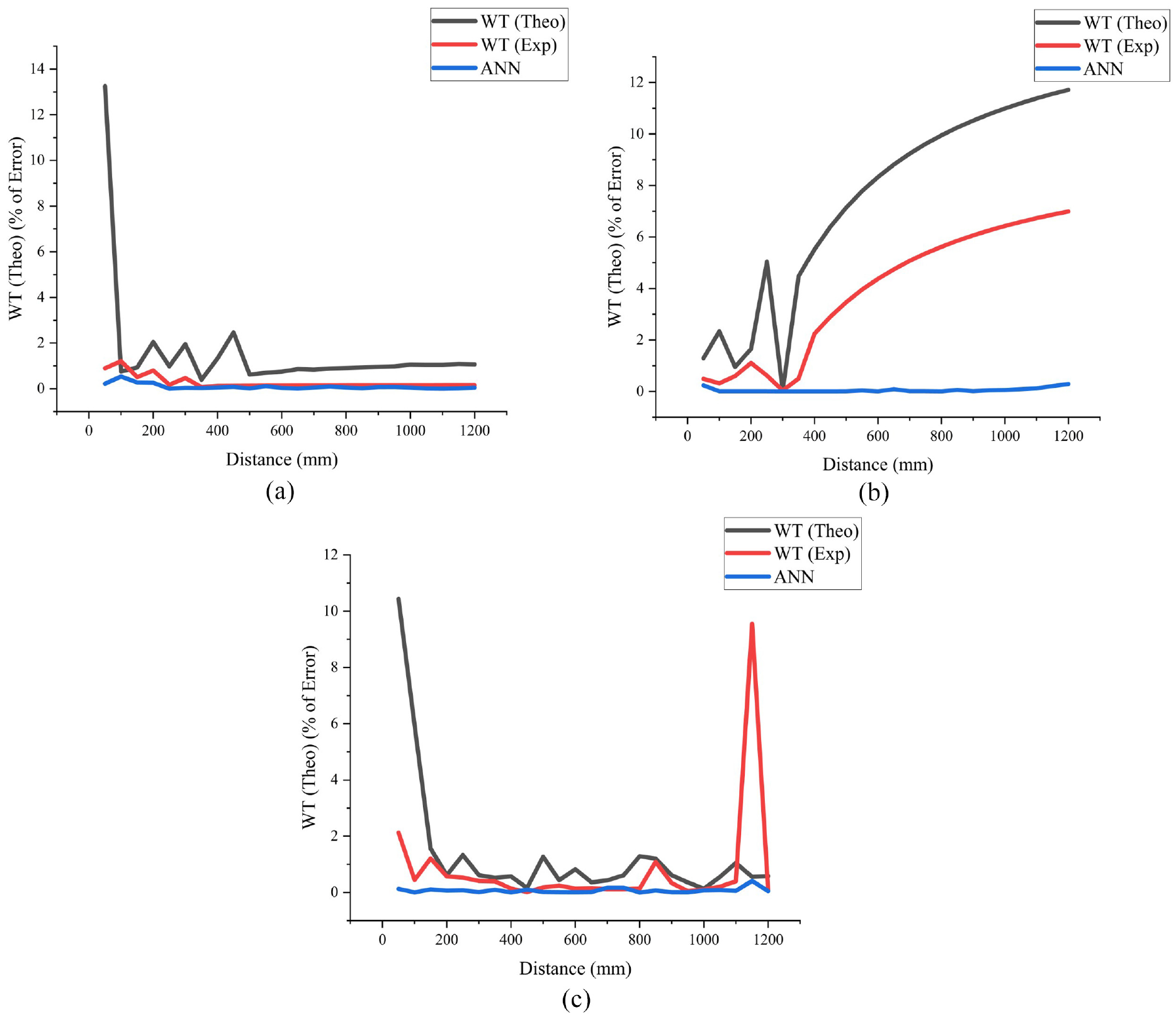
Graphical representation of error % with distance for (a) rail head, (b) rail web and (c) rail bottom flange.

Conclusion

A novel AE source localisation approach using ANN is proposed in this study. The ANN model uses fundamental characteristics of AE signals to predict the AE sources from different segments of the rail section. WT-based localisation is done with the combination of UPV for in situ determination of wave velocities and compared with existing WT techniques and ANN. The investigation shows that the present method is more accurate than the theoretically calculated wave velocities, regardless of the longitudinal and transverse placements of the AE sensors. The comparison with the WT technique shows that the developed ANN model predicts the damage more accurately than the WT technique. The developed ANN model has the potential to be utilised in real-life scenarios to localise AE sources in the rail sections without violating the traffic.

Footnotes

Acknowledgements

This research is supported by DST TSDP, Govt. of India. The authors show their gratitude and special thanks to Indian Railways, Section Engineer Mr Deepak Kumar, Assistant Engineer, Durgapur.

Declaration of conflicting interests

The author(s) declared no potential conflicts of interest with respect to the research, authorship and/or publication of this article.

Funding

The author(s) received no financial support for the research, authorship and/or publication of this article.

ORCID iD

Tamal Kundu

References

Kundu

. Acoustic source localisation. Ultrasonics 2014; 54(1): 25–38.

Bassim

. Detection of fatigue crack propagation with acoustic emission. NDT & E Int 1992; 25(6): 287–289.

Han

Carpinteri

, et al. Localisation of acoustic emission sources in structural health monitoring of masonry bridge. Struct Control Health Monit 2015; 22: 314–329.

Carpinteri

Lacidogna

Niccolini

. Critical behaviour in concrete structures and damage localisation by acoustic emission. Key Eng Mater 2006; 312: 305–310.

Sengupta

Datta

Topdar

. Structural damage localisation by acoustic emission technique: a state of the art review. Lat Am J Solids Struct 2015; 12: 1565–1582.

Kundu

Datta

Topdar

, et al. Optimal location of acoustic emission sensors for detecting rail damage. Proc Inst Civ Eng-Struct Build. Epub ahead of 10 October 2022. DOI: 10.1680/jstbu.21.00074.

Sengupta

Roy

Topdar

, et al. Investigation of layered composite plates under acoustic emission using an appropriate finite element model. Can J Civ Eng 2021; 48(12): 1639–1651.

Ono

. Application of acoustic emission for structure diagnosis. Diagnostyka 2011; 2(58): 3–18.

Roy

Sengupta

Topdar

, et al. On the applicability of wavelet transform in localising defect in a small plate using AE technique: an experimental study. In: de Oliveira Correia

JAF

Choudhury

Dutta

(Eds.) International conference on advances in structural mechanics and applications. Springer, Cham, 2023, pp. 226–237.

10.

Das

Leung

. Power spectral entropy of acoustic emission signal as a new damage indicator to identify the operating regime of strain hardening cementitious composites. Cem Concrete Compos 2019; 104: 103409.

11.

Das

Suthar

Leung

. Machine learning based crack mode classification from unlabeled acoustic emission waveform features. Cem Concrete Res 2019; 121: 42–57.

12.

Shahidan

Pulin

Bunnori

, et al. Damage classification in reinforced concrete beam by acoustic emission signal analysis. Constr Build Mater 2013; 45: 78–86.

13.

Das

Leung

. A fundamental method for prediction of failure of strain hardening cementitious composites without prior information. Cem Concr Compos 2020; 114: 103745.

14.

Clark

. Rail flaw detection: overview and needs for future developments. NDT & E Int 2004; 37(2): 111–118.

15.

Wevers

. Listening to the sound of materials: acoustic emission for the analysis of material behaviour. NDT & E Int 1997; 30(2): 99–106.

16.

Zhang

Feng

Wang

, et al. An analysis of the simulated acoustic emission sources with different propagation distances, types and depths for rail defect detection. Appl Acoust 2014; 86: 80–88.

17.

Murav’ev

Bekher

. A novel technique of AE signal processing for upgrading the accuracy of flaw localization. Russ J Nondestr Test 2002; 38(8): 600–610.

18.

Hamstad

O’Gallagher

Gary

. Modeling of buried monopole and dipole sources of acoustic emission with a finite element technique1999; 17(3/4): 97–110.

19.

Hamstad

O’Gallagher

Gary

. Examination of the application of a wavelet transformation to acoustic emission signals: Part 2. source location. J Acoust Emiss 2002; 20: 62–82.

20.

Hamstad

O‘Gallagher

Gary

. A wavelet transform applied to acoustic emission. J Acoust Emiss 2002; 20: 39–61.

21.

Hamstad

. Some observations on Rayleigh waves and acoustic emission in thick steel plates. J Acoust Emiss 2009; 27: 114–136.

22.

Anastasopoulos

Bollas

Papasalouros

, et al. Acoustic emission on-line inspection of rail wheels. In: Proceedings of European Conference Acoustic, Emission Testing, Vienna, 8–10 September 2010, pp. 1–8. Bad Breisig, Germany: NDT.net. https://www.ndt.net/article/ewgae2010/papers/76_Anastasopoulos. https://www.ndt.net/search/docs.php3?id=9758pdf

23.

Bassim

Lawrence

Liu

. Detection of the onset of fatigue crack growth in rail steels using acoustic emission. Eng Fract Mech 1994; 47(2): 207–214.

24.

Bruzelius

Mba

. An initial investigation on the potential applicability of acoustic emission to rail track fault detection. NDT & E Int 2004; 37(7): 507–516.

25.

Kuang

KSC

Koh

. Rail crack monitoring based on Tsallis synchrosqueezed wavelet entropy of acoustic emission signals: a field study. Struct Health Monit 2018; 17(6): 1410–1424.

26.

Sengupta

Roy

Topdar

, et al. Investigation of layered composite plates under acoustic emission using an appropriate FE model. Can J Civ Eng 2021; 48(12): 1639–1651.

27.

Viktorov

Mason

. Rayleigh and Lamb Waves- Physical Theory and Applications (Book on Rayleigh and Lamb waves covering generation and analysis techniques, ultrasonic flaw detection applications, propagation, etc), Springer US, 1970.

28.

Kuang

KSC

Koh

. Acoustic emission source location and noise cancellation for crack detection in rail head. Smart Struct Syst 2016; 18(5): 1063–1085.

29.

IS 13311. Non-destructive testing of concrete–Methods of Test-Part 1: Ultrasonic pulse velocity, Manak Bhavan, New Delhi, India: Bureau of Indian Standards (BIS), 1992.

30.

Bungey

Grantham

. Testing of concrete in structures. London: CRC Press, 2006.

31.

Iyer

Sinha

. Segmentation of pipe images for crack detection in buried sewers. Comput-Aided Civ Infrastruct Eng 2006; 21(6): 395–410.

32.

Chen

Zhou

, et al. An acoustic-homologous transfer learning approach for acoustic emission–based rail condition evaluation. Struct Health Monit 2021; 20(4): 2161–2181.

33.

Jingpin

Bin

Cunfu

. Acoustic emission source location methods using mode and frequency analysis. Struct Control Health Monit 2008; 15(4): 642–651.

34.

Ngui

Leong

Hee

, et al. Wavelet analysis: mother wavelet selection methods. Appl Mech Mater 2013; 393: 953–958.

35.

Zhang

Zou

Wang

, et al. A new rail crack detection method using LSTM network for actual application based on AE technology. Appl Acoust 2018; 142: 78–86.

36.

Cheng

Xin

Groves

, et al. Acoustic emission source location using Lamb wave propagation simulation and artificial neural network for I-shaped steel girder. Constr Build Mater 2021; 273: 121706.

37.

Ebrahimkhanlou

Salamone

. A deep learning approach for single-sensor acoustic emission source localisation in plate-like structures. In: Proc. 11th Int. Work. Struct. Heal. Monit. Real-Time Mater. State Aware. Data-Driven Saf. Assur 2.39, 2017, pp. 2139–2146.

38.

Chlada

Prevorovsky

Blahacek

. Neural network AE source location apart from structure size and material. J Acoust Emiss 2010; 28(1): 99–108.

39.

Vallen

. Latest improvements on freeware AGU-Vallen-wavelet. In: Proceedings of 31st conference of EWGAE (EWGAE 2010), Vienna, 8–10 September 2010, pp. 1–8 https://www.ndt.net/search/docs.php3?id=9760.

40.

Ifeachor

Jervis

(2002). Digital signal processing: a practical approach. Pearson Education. https://www-elec.inaoep.mx/~jmram/Digital_Signal_Processing__LI_TAN.pdf

41.

Zhang

Yan

, et al. Defect detection and location in switch rails by acoustic emission and Lamb wave analysis: a feasibility study. Appl Acoust 2016; 105: 67–74.

42.

Kundu

Roy

Datta

, et al. Health monitoring of Indian rail section using AE technique combined with UPVM: an experimental study. J Struct Eng 2022; 49(1): 47–58.

Development of a novel real-time AE source localisation technique using ANN for health monitoring of rail section: an experimental study

Abstract

Keywords

Introduction

Methodology

WT-based localisation

WT-based localisation using theoretical velocity

Localisation using WT and UPV

ANN-based localisation

Experimental setup

Experimental studies

Result and discussion

WT-based localisation with theoretical velocities

ANN-based localisation

Conclusion

Footnotes

Acknowledgements

Declaration of conflicting interests

Funding

ORCID iD

References