
Abstract
This article presents a robust methodology for long-term offshore structural health monitoring (SHM) using the Global Navigation Satellite Systems (GNSS). The methodology relies on recently developed regional reference frames and single-receiver phase-ambiguity-fixed Precise Point Positioning techniques. The stable Gulf of Mexico Reference Frame 2020 (GOM20) provides a robust and consistent reference system for long-term offshore SHM in the Gulf of Mexico (GOM). Continuous GNSS observations (DEV1, 2010–2020) on a fixed platform in the Eugene Island 330 oil field are used to illustrate the methodology. The platform was installed in 1982 in 82-m water about 130 km away from the Mississippi Delta coastline. The major monitoring items include horizontal movements, seafloor subsidence, structure submergence, and seasonal oscillations. The stand-alone GNSS monitoring achieves 3- to 4-mm root-mean-square accuracy in the horizontal direction and 7 mm in the vertical direction for daily positions in the GOM region. According to this study, the GNSS antenna (DEV1) has moved 6 cm toward the northeast with respect to GOM20 since 2010; the ongoing structure submergence rate in the Eugene Island 330 oil field area is approximately 15 mm/year, a combination of seafloor subsidence (12 mm/year) and sea-level rise (2.6 mm/year) with respect to GOM20. The submergence in the future 40 years (2021–2060) would be greater than 0.6 m, likely between 0.8 and 1.0 m, but is unlikely to exceed 1.3 m. The peak-to-trough amplitudes of the seasonal movements at the top of the platform are below 5 mm in all three directions, comparable with the seasonal movements recorded by onshore GNSS in the Louisiana coastal region. The methodology introduced in this article can be applied to SHM in other offshore regions where stable regional reference frames are available.
Keywords
Introduction
Motivation
Offshore platforms are the critical infrastructure for offshore oil and gas exploration and production. As the offshore infrastructure ages and grows ever more complex, the need for long-term, continuous, and robust structural stability and integrity monitoring is imperative to ensure optimal performance and the potential for life extension. Long-term stability monitoring of civil engineering structures is an essential element of the broad structural health monitoring (SHM). SHM has become a multidisciplinary and cross-disciplinary research field encompassing civil engineering, mechanical engineering, structural dynamics, surveying, signal processing, computational hardware and software, data telemetry, smart sensors, machine learning and pattern recognition, remote sensing (ground-based, drone-based, satellite-based), as well as other fields yet to be defined.1,2 Global Positional System (GPS), Global Navigation Satellite Systems (GNSS) in general, has become a crucial tool for onshore SHM.3–6
As of the 2010s, the applications of GNSS in SHM are primarily limited to kinematic positioning for short-term monitoring (a few hours to days), studying the dynamic behaviors of structures (e.g., long-span bridges, high-rise buildings).7–13 Static GNSS techniques have been widely applied in long-term geological hazards monitoring (e.g., volcanos, faulting, landslides, subsidence) during the past two decades. In contrast, GNSS techniques have rarely been used for long-term offshore SHM. The reasons will be discussed later. This study aims to promote the application of long-term GNSS monitoring techniques in offshore SHM.
Common problems
GNSS receivers record complex observations of ranges and phases between the GNSS antenna and each of visible satellites, and the positions of these satellites. Surveying-level GNSS receivers do not directly provide position measurements. Extensive calculations are required to obtain high-accuracy high-precision coordinates of a GNSS antenna. GNSS positioning algorithms generally implement two approaches to achieving high-precision GNSS positions: relative and absolute positioning.14,15 A relative positioning method uses simultaneous observations from two or more GNSS units; at least one of these antennas should be fixed at a known location. The position of a rover station can be determined relative to the fixed station by applying a carrier-phase double difference (DD) method. In contrast to the DD method, the absolute method involves only one GPS station to determine its coordinates with respect to a global reference frame. Several investigators have compared the performance of the two methods in SHM.16–18 The DD method has been successfully applied in onshore and near-offshore (e.g., <50 km) SHM.19–21 However, it is a challenge to apply the DD method for far-offshore (e.g., >100 km) and long-term (many years to decades) SHM.
The DD method requires at least one reference GNSS, which is required to collect data simultaneously with the rover station. The rover’s positions cannot be solved at the time that the base GNSS has no data. The accuracy of the rover’s positions heavily depends on the distance between the reference and rover, known as baseline. However, deep-water (e.g., deeper than 100 m) offshore platforms are often at several 100 km away from the coastline. The accuracy and precision of DD positioning degrade with the increase in the baseline length. 22 The costs for operating reference stations in a long term (many years to decades) could also be high. Furthermore, the stability of the reference station itself needs to be justified independently. In practice, the assessment of the stability of reference stations could be tricky and complex since many coastal regions are suffering from coastal subsidence associated with onshore and offshore fluid (groundwater, oil, and gas) withdrawals, as well as natural compaction of unconsolidated young sediments.23,24 Subsidence at rover sites will be underestimated if the reference station is subsiding.
The continuity and stability of reference stations and the baseline length have become key issues limiting the applications of GNSS (specifically, the DD positioning method) in offshore SHM. This article aims to introduce a methodology that does not require any land-based reference GNSS for conducting high-accuracy and long-term offshore SHM. The method is simply called stand-alone GNSS monitoring.
Needs of offshore SHM within the Gulf of Mexico
The Gulf of Mexico (GOM) region is one of the most important petroleum production regions in the world due to giant oil and gas reservoirs along the coast and offshore. The U.S. portion of the GOM offshore region has been the heart of the U.S. energy industry, making up about 15% of total U.S. crude oil production and about 5% of total U.S. dry natural gas production as of 2021. 25 Oil and gas structures in the GOM region have created a large and complex network of standing structures, interconnected by hundreds of miles of pipelines (Figure 1). Over 6000 oil and gas structures (rigs or platforms) have been installed in the GOM since the first offshore drilling began in 1942. These structures range in size from single well caissons in shallow water (a few meters) to extensive, complex facilities in deep water over 3000 m. As of 2020, about 3500 platforms stand in the U.S. portion of GOM (Figure 1), and over 3200 platforms remain active. 26
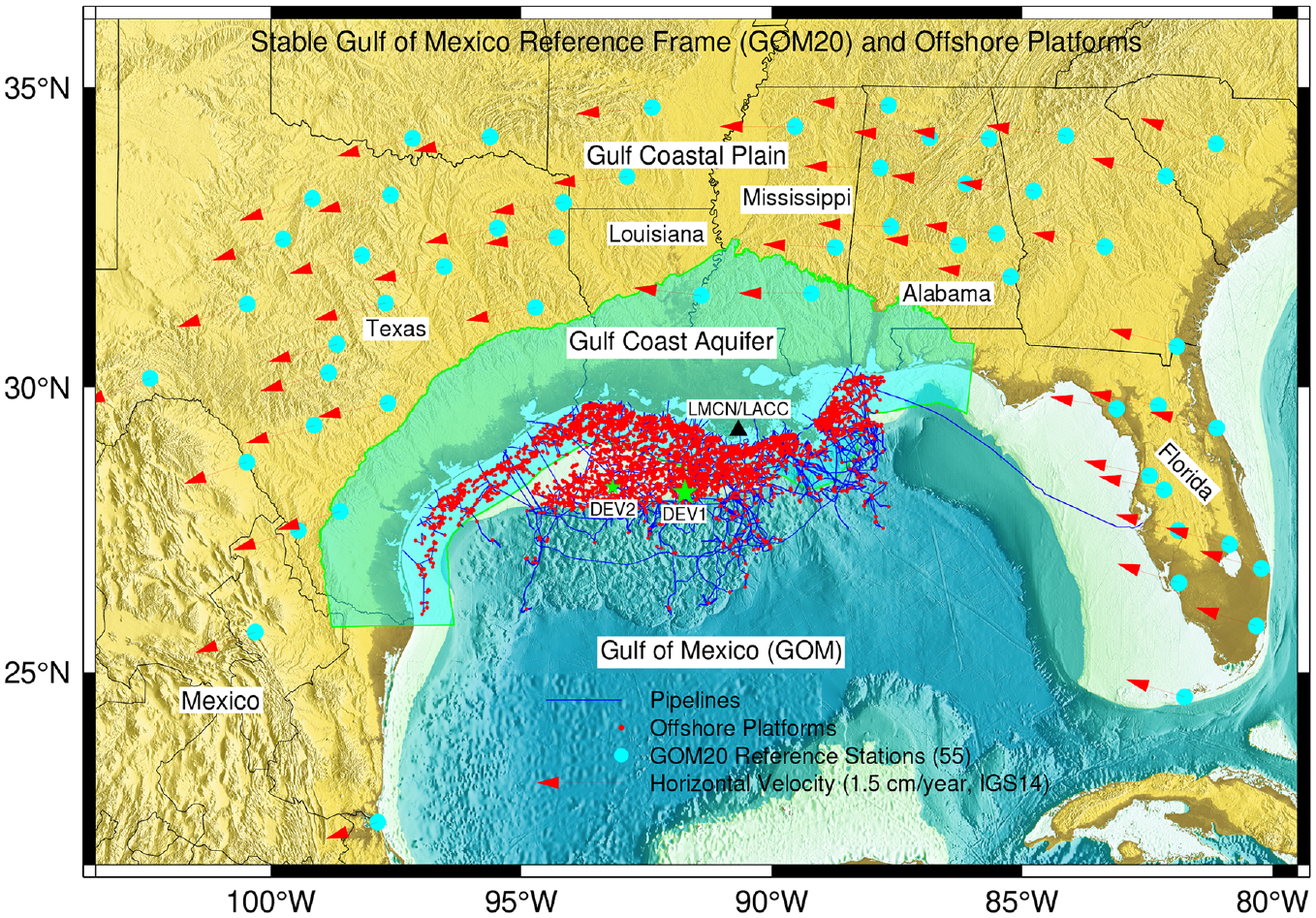
Map showing the locations of the 55 reference stations for realizing the stable Gulf of Mexico Reference Frame 2020 (GOM20), and offshore platforms and pipelines in the Gulf of Mexico (GOM).
Many offshore platforms in the GOM were built in the 1970s and 1980s, approaching 40 years or even older as of the 2020s. They have reached or exceeded their original design life. Conducting continuous and high-accuracy SHM is essential for the safe operation of these offshore oil and gas facilities.
Case study data
The National Geodetic Survey (NGS) and the Louisiana State University (LSU) installed two GNSS stations (DEV1 and DEV2; Figure 1) on two platforms near the Louisiana coast in 2009 for water vapor studies. 29 The raw data are available through the LSU Center for GeoInformatics and NGS. DEV1 is installed on a fixed platform in the Eugene Island block 337 (abbreviated as E.I. 337) (Figure 2), a portion of the Eugene Island 330 oilfield. The fixed platform (E.I. 337-A) was built in 1982, about 130 km away from the frontier of the Mississippi Delta and 270 km southwest of New Orleans. The water depth is approximately 82 m at this site. The actual deck height was about 15 m above the water level (as of the late 2010s), standing on six steel legs piled into the seafloor. According to the NGS Online Positioning User Service solution, the elevation of the GNSS antenna is 34.38 m (as of April 2020), referred to the North American Vertical Datum of 1988 (NAVD 88). The first production started in October 1984. DEV1 has been continuously operated for about one decade (2010–2020), providing an outstanding opportunity to develop the methodology for offshore SHM.
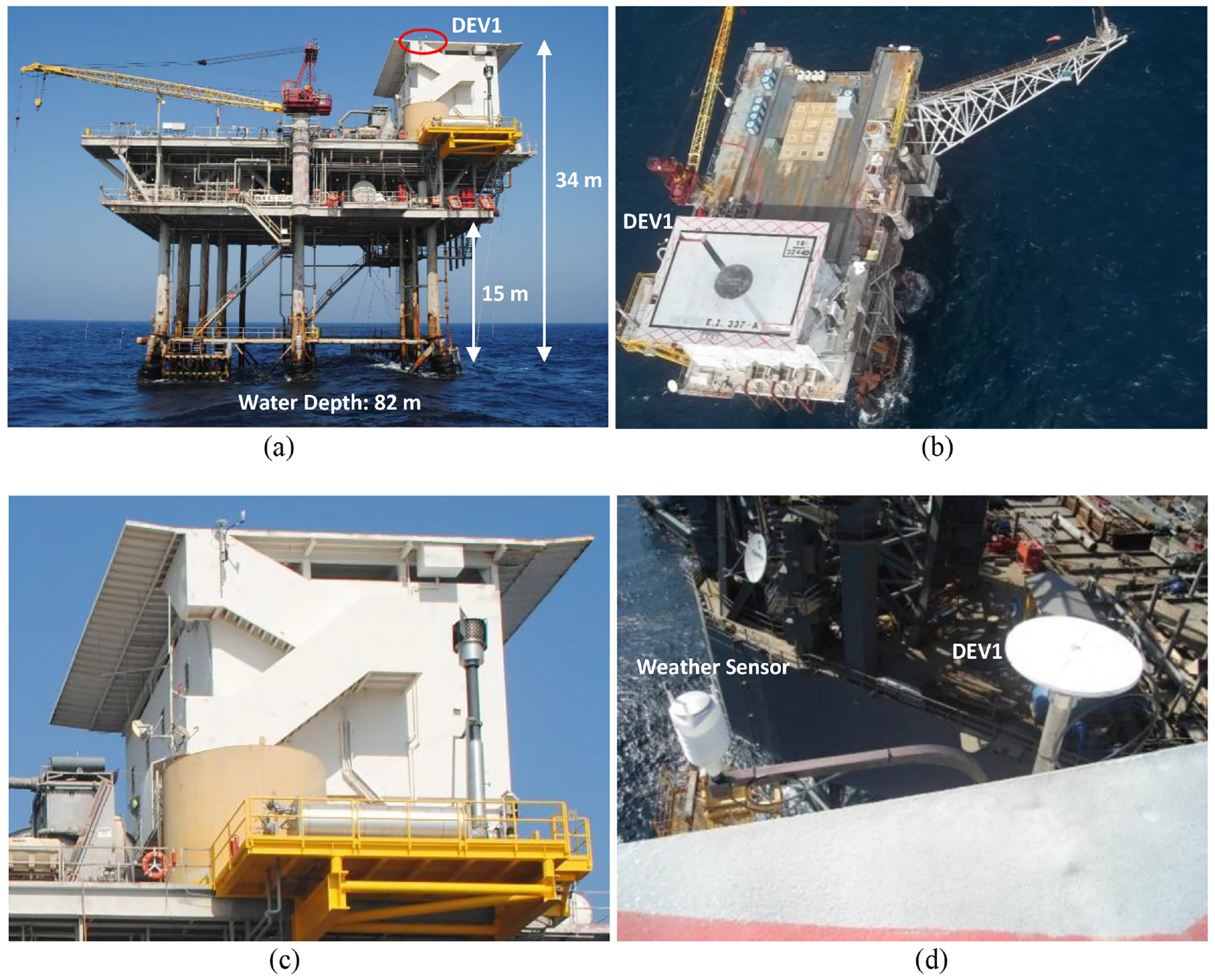
The Eugene Island block 337 platform A (E.I. 337-A) and the permanent GNSS antenna DEV1. (a) A westside view of the platform; (b) a top view of the platform; (c) the locations of the GNSS antenna (DEV1) and the weather sensor; (d) a top view of the GNSS antenna (Trimble Zephyr Geodetic II) and the weather sensor.
Both GNSS receivers at DEV1 and DEV2 sites were configured to collect satellite signals at a rate of 1 s per sample. This allows research to study the kinematic movements of the platforms, particularly during hurricane seasons. For static positioning to get daily solutions, the 1 s per sample data were resampled to 15 s per sample for data archiving, and post-processing software packages further down sample the 15 s per sample data by a factor of 4 or even larger. To get high-accuracy positions, the final satellite orbit data provided by the International GNSS Service (IGS) (https://igs.org/products) rather than the satellite positions recorded in the GNSS receivers are used.
DEV2 was installed on a platform within the West Cameron Block 560 in early 2010. Unfortunately, this station was decommissioned for uncontrollable reasons in early 2012. The GNSS observational history at DEV2 was approximately 2 years. Figure 3 illustrates the 2-year displacement time series derived from DEV2 and DEV1. The detailed methods for GNSS data processing will be discussed in the next section. It appears that the measures at DEV2 are noisier than the measures at DEV1. It is likely that the DEV2 antenna (therefore the platform) experienced slightly larger oscillations than the DEV1 antenna. The decadal GNSS data at DEV1 indicate that the platform experienced a few millimeters per year horizontal movements and over 1 cm/year vertical movements during the past 10 years. Unfortunately, it is hard to detect the gradual movements at a few millimeters per year within a 2-year time window, as shown in Figure 3. In general, it requires over 3 and 5 years of continuous GNSS observations to achieve submillimeter per year (<1 mm/year) uncertainty (95% confidence interval (CI)) for horizontal and vertical site velocity estimates, respectively. 30
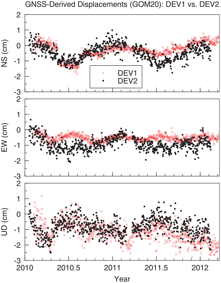
GNSS-derived three-component displacement time series at DEV1 and DEV2 during the lifetime of DEV2 (2010–2012). The displacements are derived from the daily Precise Point Positioning (PPP) solutions with respect to the stable Gulf of Mexico Reference Frame 2020 (GOM20).
Methodology
In geodesy and surveying engineering, the term GNSS has become the standard generic term for high-accuracy satellite positioning systems, including GPS, GLONASS, Galileo, BeiDou, and other regional satellite-navigation systems. The DEV1 site was equipped with the Trimble antennas and receivers and recorded GPS signals throughout its entire history (2010–2020). DEV1 started to record GLONASS signals in 2018. This study only used GPS signals in calculating the daily positions. The methodology developed through this article is applicable to the observations from other satellite systems. Accordingly, the umbrella term GNSS is used throughout this article.
The stand-alone positioning has been successfully utilized in long-term geological hazards monitoring31–35 and onshore SHM16,36 because of its operational simplicity and the consistency of the positioning accuracy over time and space. The methodology proceeds in five steps: (1) obtaining the Earth-Centered-Earth-Fixed (ECEF) Cartesian coordinates (XYZ) with respect to a global reference frame from GNSS raw data, (2) transforming the ECEF-XYZ coordinates from the global reference frame to a regional reference frame, (3) removing outliers and steps and converting the ECEF-XYZ coordinates to a site-specific topocentric coordinate system: East–North–Up (ENU), (4) conducting decomposition analysis for the ENU time series, and (5) projecting future structure submergence.
Regional reference frame
GNSS positions are initially provided ECEF-XYZ coordinates with respect to the current global geodetic reference frame, which is the IGS 2014 (IGS14) as 2021. 37 IGS14 is based on the International Terrestrial Reference Frame 2014. 38 In general, a global geodetic reference frame is a no-net-rotation reference frame, which is realized by minimizing the overall horizontal movements of a group of selected reference stations distributed worldwide. As a result, GNSS-derived site movements with respect to a global reference frame are dominated by long-term drift and rotation of tectonic plates. For example, GNSS stations in the GOM region retain about 2 cm/year horizontal movement toward the southwest with respect to IGS14 (see Figure 1), and approximately 1 mm/year upward movement. The common motions, also referred as background signals, at a few centimeters per year often obscure site-specific ground or structural displacements (or deformation) at a few millimeters per year. To precisely monitor land subsidence, faulting, and sea-level rise (SLR) within the GOM region, the author and his team established the stable Gulf of Mexico Reference Frame in 2020, abbreviated as GOM20. 39 GOM20 will be periodically updated (every 4–5 years) and synchronized with the future updates of the IGS reference frame.
GOM20 is realized by 55 long-history (>8 years, 13.5 years on average) permanent GNSS stations fixed on the Gulf Coastal Plain, a stable portion of the North American plate (Figure 1). Those stations were selected from over 1000 Continuously Operating Reference Stations (CORS) within the pan GOM region. They were not affected by localized fault movements and land subsidence. The frame stability of GOM20 is approximately 0.3 mm/year in the horizontal (north-south (NS), east-west (EW)) directions and 0.5 mm/year in the vertical direction. The regional reference frame minimizes the regional common movements, such as the secular movements of the North American plate, glacial isostatic adjustments, and the part of natural subsidence. Thus, it highlights the local-scale movements, such as the anthropogenic subsidence, faulting, and structural deformation.
A sophisticated regional geodetic infrastructure includes three components: a dense continuous GNSS network (hardware), a stable regional reference frame (firmware), and software packages for millimeter-accuracy positioning (software).40,41 The hardware means long-term continuous GNSS stations in the region and their recorded datasets. The firmware is developed from the hardware but is relatively independent. It requires a long-term (e.g., >7 years) accumulation of continuous GNSS observations from a regional CORS network to establish a rigorous regional reference frame.42,43
Daily PPP solutions
Precise Point Positioning (PPP) is a typical absolute positioning method, which solves millimeter-accuracy positions from a single GNSS unit. 44 PPP heavily relies on precise GNSS satellite clock and orbit corrections, generated from a network of global GNSS stations. The recently developed single-receiver phase-ambiguity-fixed PPP algorithms have significantly improved the positioning accuracy.45,46 The initial coordinates of the PPP solutions are aligned to the global reference frame that defines the global coordinates of satellite orbits, which is IGS14 as of 2021.
The PPP method has been integrated into several scientific GPS software packages, such as the GipsyX/RTGx (previously GIPSY/OASIS) software developed by the Jet Propulsion Laboratory, United States (JPL), 47 the Bernese GNSS software developed by the Astronomical Institute of the University of Bern, Swiss, 48 and the PRIDE software 49 developed by the Wuhan University, Wuhan, China . In this study, we use the single-receiver phase-ambiguity-fixed PPP employed in the GipsyX/RTGx (V 1.7) software package for daily GNSS data positioning. The detailed setup for the PPP processing is the same as the setup for the HoustonNet GNSS data routine processing. 50
Reference frame transformation
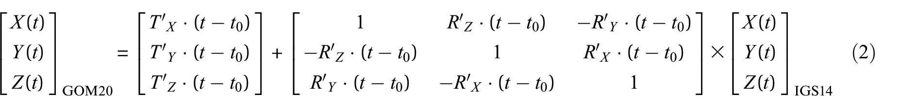
In geodesy, the Helmert transformation is often used to transform a set of points (described by three vectors) at a specific epoch from one reference frame into another reference frame. The Helmert transformation is also called as a seven-parameter transformation, which can be described as:

where
The PPP processing generates the ECEF-XYZ coordinates with respect to the global reference frame IGS14, which can be transformed to GOM20 according to the following equation 39 :
where
Seven parameters for ECEF-XYZ coordinate transformation from IGS14 to GOM20.
ECEF: Earth-Centered-Earth-Fixed; GOM20: Gulf of Mexico Reference Frame 2020; IGS14: International GNSS Service 2014.
Seven parameters for transforming ECEF-XYZ coordinates from IGS14 to GOM20 according to Equation (2). 39
To study displacements at the Earth’s surface, the ECEF-XYZ coordinates are converted to a geodetic coordinate system (longitude, latitude, and ellipsoid height) referencing to the Geodetic Reference System 1980 ellipsoid . The longitude, latitude, and ellipsoidal height are then converted to a site-specific topocentric coordinate system (ENU) for tracking displacements in the NS, EW, and up–down (UD) directions. The displacement in the UD direction represents the change of ellipsoid heights over time. In practice, the vertical displacement (subsidence or uplift) obtained from ellipsoid heights is the same as the vertical displacement derived from orthometric heights. 51 The following matrix equation is used to calculate the ENU displacement time series at each site:
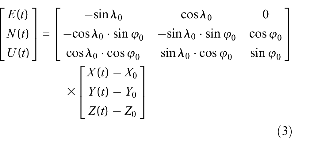
where
Figure 4 illustrates the ENU displacement time series at DEV1 with respect to the global reference frame IGS14 and the regional reference frame GOM20. The horizontal site velocities are 3.9 ± 0.5 mm/year (NS) and −8.8 ± 0.2 mm/year (EW) with respect to IGS14, and 4.9 ± 0.5 mm/year (NS) and 2.5 ± 0.2 mm/year (EW) with respect to GOM20. Throughout this article and unless specifically stated otherwise, the uncertainty of a site velocity (rate) is quantified using ±95% CI, which is often considered as a very likely range. The velocities in the EW direction are significantly different, approximately 1 cm/year. The IGS14 velocity of 8.8 mm/year toward west does not reflect local movements. The site velocities with respect to GOM20 indicate that the DEV1 antenna has moved about 6 cm toward the northeast direction since 2010. The vertical displacement rates with respect to IGS14 and GOM20 are −12.8 ± 0.4mm/year and −11.7 ± 0.4 mm/year, respectively. The site velocities with respect to GOM20 can be tied to a physical object, the stable Gulf Coastal Plain (see Figure 1). However, the site velocities with respect to IGS14 cannot be tied to any specific physical objects. It could be problematic to assess the stability of civil structures using site velocities with respect to IGS14. GNSS users are obliged to select the right reference frame for their specific monitoring purposes.
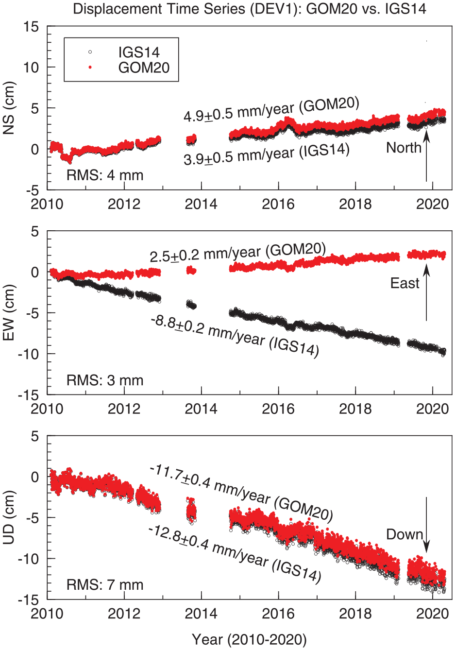
GNSS-derived three-component (ENU) displacement time series at DEV1 with respect to the global reference frame IGS14 and the regional reference frame GOM20.
Identification of outliers and steps
Although the positional accuracy and precision (repeatability) of GNSS solutions have been improving over time, certain large variations are often superimposed into the daily coordinate time series. These obvious anomalies are often referred to as outliers. They do not reflect the actual physical motions of the antenna. Removing outliers is necessary before conducting further data processing and analysis, particularly for assessing site velocities obtained by a least squares regression. The operation of permanent GNSS stations often involves antenna and receiver changes, as well as the update of receiver firmware and the replacement of antenna cables. These changes could result in abrupt steps in the GNSS position time series. The operator of DEV1 maintains a detailed field log, tracking all antenna, receiver, cable, and firmware changes. No considerable steps (>5 mm) are detected after correcting all equipment-change-related position shifts.
In this study, the outliers are identified and removed in the IGS14-XYZ time series before conducting reference frame transformation and calculating the ENU position time series. The method employs multi-step processes to progressively identify and remove outliers, not just a single threshold. The detailed method is addressed in a recent publication. 50 About 50 daily positions among 2948 days (1.5%) are removed as outliers. Further analysis indicates that the majority of outliers occurred in those days that only had a few hours of observations (e.g., less than 4 h). Equipment maintenance and loss of power supplies were the main reasons causing these short observations. Extreme weather conditions could also cause outliers, such as heavy rainfalls accompanied by the passage of weather front continuing for several hours. 31
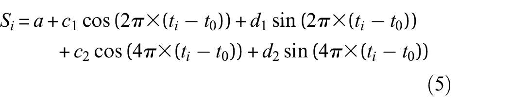
Decomposition and seasonal modeling
Seasonal oscillations, both in the horizontal and vertical directions, have been widely observed from onshore GNSS-derived displacement time series. The seasonal motions are often associated with seasonal changes of temperature, terrestrial hydrosphere, atmospheric pressure, precipitation (soil moisture), fluctuation of groundwater levels, and modeling errors in GNSS positioning. The step-free GNSS time series

where
where
The amplitude of the annual seasonal signals can be measured by
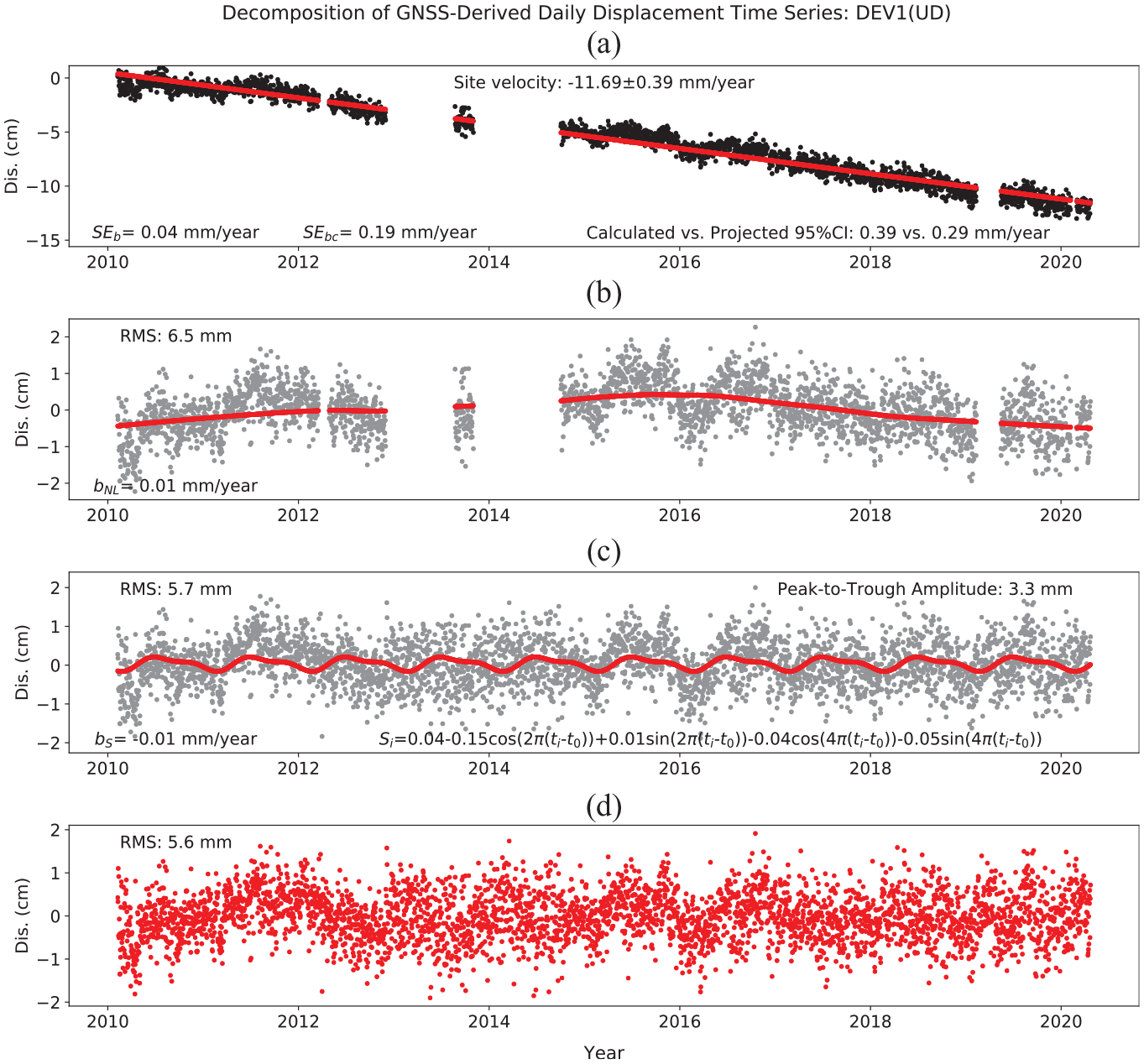
The decomposition results of the GNSS displacement time series (DEV1, UD) with respect to GOM20. The details of these parameters are addressed in the reference. 53 (a) Displacements y(i) and the linear component L(i), (b) nonlinear component NL(i), (c) seasonal component S(i), and (d) residuals r(i).
Uncertainty assessments
The accuracy of both positioning and site velocities has been continuously improved over the past decades because of advances in GNSS hardware (receivers, antennas, satellites), software, and the availability of regional reference frames. PPP results in 24-h average positions from the daily observational files. Each file of each station is processed independently. Thus, the daily positions are insulated from potential data problems or real movements at other days or other stations. This is a big advantage of the stand-alone positioning method compared to the relative positioning method. However, it does not mean that the PPP daily positions are statistically independent. In fact, the errors superimposed into the GNSS time series are autocorrelated; that is, the error in each measurement is correlated with the errors in other measurements. The autocorrelated errors complicate the uncertainty analysis of both positions and site velocities. 30
Repeatability of daily positions
The root-mean-square (RMS) of the de-linear-trended GNSS time series is often used to assess the repeatability of GNSS positioning. 54 The RMS estimate is also called RMS accuracy since it somehow indicates the repeatability of the displacement measurements. The RMS accuracy has improved significantly during the past two decades with the continuous improvement of global and regional geodetic infrastructures. Bertiger et al. 47 reported that the GipsyX-PPP daily resolutions achieve approximately 2–3 mm global RMS accuracy in the horizontal direction and 6–7 mm in the vertical direction. According to the previous study in the GOM region,15,50 the accuracy of the PPP solutions in the GOM coastal region is slightly worse than the global average, mostly because of the humid climates. The RMS accuracy for the daily positions at DEV1 is 4 mm in the NS direction, 3 mm in the EW direction, and 7 mm in the vertical direction (Figure 4).
The uncertainties of site velocities
For long-term site stability assessment and risk analysis, users mostly rely on GNSS-derived site velocities, not the absolute positions or displacements. Site velocities have become the primary products for long-term GNSS monitoring. Nevertheless, a site velocity must be used with a full understanding of its uncertainty. Uncertainties of field measures and modeled parameters are always critical for offshore structural reliability assessment. 55 In general, accurate positions do not guarantee to obtain reliable velocity estimates. The uncertainty of a site velocity estimate does not entirely depend on the hardware (antennas and receivers), but largely relies on the length of the time span of observations and the stability of the regional reference frame.
There are sophisticated mathematical methods for calculating the linear trend and its uncertainty for stationary time series in statistics. However, GNSS time series often exhibit nonstationary behaviors, such as nonlinear motions, seasonal motions, and random walks. Consequently, the uncertainty estimated with the conventional method is unrealistically small and significantly underestimates the real uncertainty. In practice, different scaling and approaches have been developed by different research groups to correct the velocity uncertainty. There is considerable disagreement over the uncertainties of GNSS-derived site velocities, which leads to confusions, even controversies, over the interpretation of site or structural stability. The author recently published an analytical methodology for determining the uncertainty of GNSS-derived site velocity.
30
This method accounts for the autocorrelation among GNSS-derived daily displacement time series. An effective sample size (
Results
Seasonal deformation
Seasonal signals observed at onshore GNSS fixed on ground surface have been heavy investigated by geophysicists. According to a recent investigation conducted by the author, the uncertainty of the amplitudes of GNSS-derived seasonal signals is below 2 mm in the Houston metropolitan region, Texas. 56
Figure 6 depicts the seasonal ground movements at DEV1 and two onshore GNSS (LMCN and LACC) . LMCN and LACC are about 160 km away from DEV1 (Figure 1). LMCN is installed on the northeast wing of the Y-shaped two-story building on the campus of the Louisiana University Marine Consortium, Cocodrie, Louisiana. LACC is a permanent GNSS installed on the northwest wing of the Y-shaped building. The distance between LMCN and LACC is about 60 m. The P2T amplitudes of the seasonal signals at DEV1 are comparable to the amplitudes observed at LACC and LMCN, except in the EW direction of LMCN. The seasonal amplitudes in the three directions of LACC and the NS and vertical direction of LMCN are comparable with the amplitudes of other GNSS in this area. A further investigation indicates that the LMCN antenna is adjacent to a piece of mental roof above the front hallway. It is likely that the significant periodical variations (P2T, 8 mm) in the EW component of LMCN were caused by site-specific multipaths rather than real oscillations of the antenna.
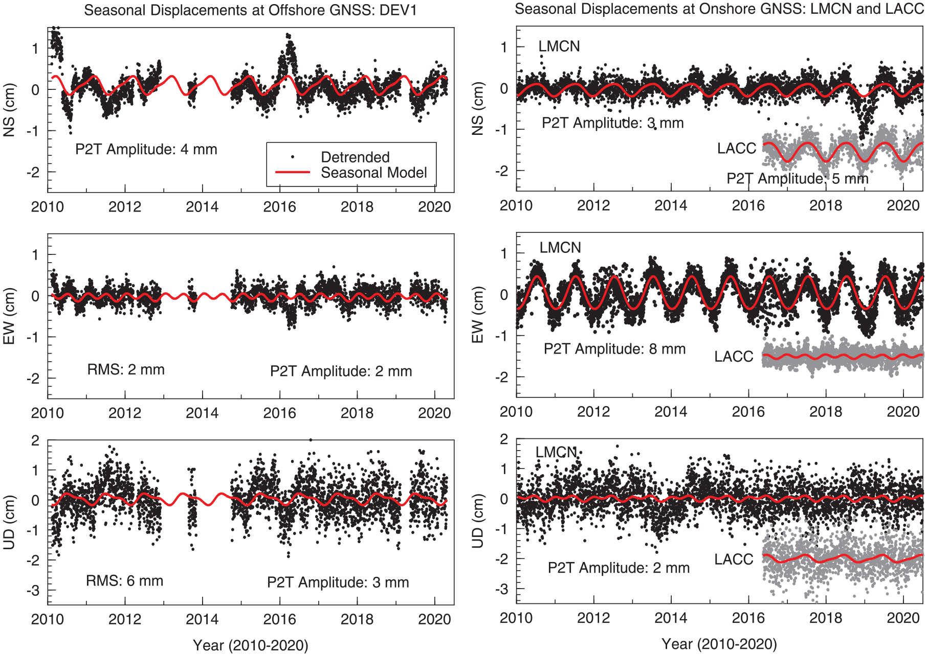
(a) Three-component seasonal signals derived from the offshore GNSS data (DEV1); (b) three-component seasonal signals derived from onshore GNSS data (LMCN and LACC).
Figure 7 depicts the vertical P2T amplitudes and site velocities (2010–2020) at about 100 coastal GNSS sites around the Mississippi delta and Louisiana coastal areas. Most GNSS stations are installed on the ground or one- to two-story office buildings. The GNSS raw data are primarily from NGS and UNAVCO. The IGS14-XYZ coordinates of a few stations are obtained from the Nevada Geodetic Laboratory. 57 The vertical P2T amplitudes at most GNSS sites are below 5 mm, comparable with the seasonal movements at the offshore platform (see Figure 6). The seafloor may experience periodical movements with the fluctuation of oil and gas production. The platform frame could also experience periodical deformation corresponding to the seasonal temperature changes. Both may contribute to the minor seasonal motions at DEV1. Overall, the amplitudes of the seasonal movements at the top of the offshore platform are similar to the amplitudes of the seasonal movements at onshore GNSS sites. That is to say, the seasonal movements of the platform frame are below the level that can be detected confidentially by the stand-alone GNSS technique.
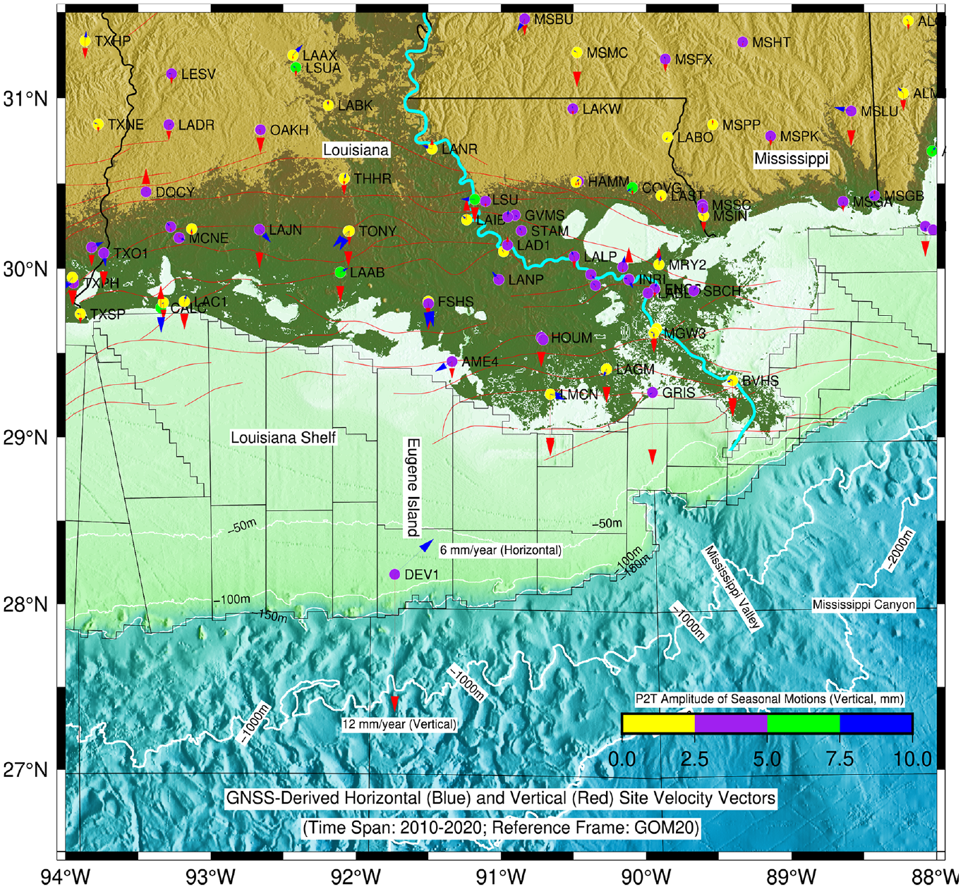
Velocity vectors and P2T amplitudes (vertical) at permanent GNSS stations (2010–2020) within the Mississippi delta and offshore.
Horizontal movements
The antenna of DEV1 has moved approximately 6 cm toward the northeast (6 mm/year) since 2010, as depicted in Figure 4. DEV1 experienced obviously more significant horizontal movements than those onshore GNSS, as shown in Figure 7. The gradual horizontal movements at the GNSS antenna (DEV1) could comprise the horizontal movement of the platform frame and the tilt of the frame over time. Seafloor subsidence associated with fluid (oil, gas, water) withdrawals could induce seabed movements toward the center of subsidence bowl. Uneven subsidence within the footprint of the platform could tilt the platform frame.
Seafloor subsidence
The production from hydrocarbon reservoirs decreases fluid pressure in the pore space and increases the stress on the rock formation. Depending on the rock strength, the increased stress could induce compaction of the reservoir, which ultimately transfers to the seafloor. Seafloor subsidence has been a significant concern for the long-term operation of offshore oil and gas facilities. Accurate and continuous seafloor subsidence monitoring provides valuable insights for assessing the safety of offshore infrastructure (platforms, pipelines), optimizing well and reservoir management, and supporting efficient hydrocarbon production decisions.
The vertical and horizontal displacement time series at DEV1 show steady displacements over the past 10 years without abrupt positional changes (Figure 4). The average subsidence rate is about 1.2 cm/year (2010–2020) with respect to GOM20. The platform was built in 1982 and the GNSS (DEV1) was installed in the end of 2009. The vertical loading had been stabilized during the three-decade operation before 2009. Thus, the vertical elastic shortening of the platform structure should have ceased before the installation of DEV1. In general, inelastic structural deformation often tends to be nonlinear over time. The high linearity of the vertical displacement time series at DEV1, as depicted in Figure 5(a), suggests that inelastic deformation of the platform frame would be minor even if it did occur. Accordingly, the GNSS-recorded subsidence should be dominated by the seafloor subsidence, comprising natural compaction of unconsolidated young sediments and the anthropogenic compaction of the oil and gas reservoir. Natural subsidence refers explicitly to the gradual compaction of unconsolidated sediments under the weight of overlying sediments and the gravity of itself.
The subsidence rates at onshore GNSS sites within the Mississippi delta and adjacent areas are depicted in Figure 7. The subsidence rates at most sites are below 3 mm/year (2010–2020) with respect to GOM20. Only a few sites in the frontier of the Mississippi Delta plain recorded subsidence rates larger than 3 mm/year. For example, the subsidence rate is 5.5 ± 0.3 mm/year at LMCN (2010–2020), 6.4 ± 0.3 mm/year at GRIS (2010–2020), 3.0 ± 0.3 mm/year at BVHS (2010–2020), and 3.0 ± 0.4 mm/year at LAGM (2014–2020) . According to numerous investigations, the ongoing subsidence in the frontier of the Mississippi Delta region is dominated by the natural compaction of young and shallow sediments, particularly the young Holocene sediments brought to the delta area by the Mississippi river.59–62 DEV1 is located on the south edge of the Louisiana shelf, over 130 km away from the frontier of the delta area. The thickness of Holocene sediments in the south edge of the shelf area is less than 10 m, 63 which are older and thinner than the Holocene sediments in the frontier of the delta area. Vertical displacement associated with deep-seated tectonic movements could also cause gradual land subsidence. 64 However, there are few active faults within the Louisiana shelf area (Figure 7). Accordingly, the natural subsidence on the continental shelf would be considerably slower than the ongoing natural subsidence in the frontier of the delta area, which is about 3–6 mm/year.
DEV1 site is adjacent to the Gulf Coast Aquifer system (see Figure 1). The depth of unconsolidated sediments in the south portion of the aquifer system retains consistency over space. The average rate of natural subsidence along the 600-km TX coastline is 1.4 mm/year with respect to GOM20. 63 The half-century tide gauge data (the 1960s–2010s) and GPS data at Sabine Pass (near TXSP, see Figure 7) indicate that the ongoing natural subsidence in the Texas-Louisiana board coastline area is approximately 2 mm/year with respect to GOM20. 65 The thickness of unconsolidated sediments at the DEV1 site is comparable with the thickness of unconsolidated sediments in the coastal area. Accordingly, the rate of ongoing natural subsidence at DEV1 would be similar to the natural subsidence in the Texas-Louisiana coastal area, approximately 2 mm/year. The remaining 1 cm/year among the total subsidence (1.2 cm/year) might be contributed by anthropogenic subsidence in responding to the reservoir pressure decrease caused by hydrocarbon withdrawals.
Submergence
The combination of seabed subsidence and SLR causes offshore structures to submerge into the water gradually. A direct consequence of the submergence is the gradual reduction in the air gap between the average sea level and the base of platform structures, which causes wave-in-deck (WID). The wave force generated from hurricane winds presents one of the greatest risks for physical damage to offshore platforms. Deck height is one of the most important characteristics in determining the safety of offshore platforms. Current regulations used in the design of offshore platforms often require a minimum air gap of 1.5 m between the expected magnitude of a 100-year wave height (as a function of water depth) and the underside of the lowest deck of the platform. 66
According to our recent investigations, 39 the average SLR rate during the past five decades within the GOM is 2.6 mm/year with respect to GOM20. The peak production of oil and gas in Eugene Island 300 oil field area occurred during the 1970s–1990s 67 ; the production since the 2000s is much lower than its peak production period. The seafloor subsidence from the 1980s to 2000s was likely more rapid than the GNSS-recorded subsidence (12 mm/year) during the 2010s. So, the ongoing 15 mm/year submergence rate is a lower estimate of the overall submergence rate. That is to say, a minimum of 60-cm submergence had occurred for the E.I. 337-A Platform during its 40-year history (1982–2021).
The loss of air gap has become a major concern for offshore operators within the GOM. Many platforms in the GOM have gone well beyond their expected life. The E.I. 337-A platform is near the very end of its operational life, as of 2020. Two platforms (E.I. 330-C and E.I. 330-B) in the Eugene Island 330 field were raised 4.25 m in 2007 using the deck-raising technology to restore the air gap. 68 There are many younger platforms in the Eugene Island area, and more platforms will be installed in the future. Projecting future submergence based on what we learned from the seafloor subsidence monitoring at DEV1 would be useful for the planning of future operation of offshore structures within the GOM.
The global sea level has been rising since the mid-1800s, and the rising rate has accelerated in recent decades due to global warming. 69 In general, faster SLR rates are projected for scenarios with higher rates of global carbon dioxide emission. Projecting the future sea level is indispensable for projecting future offshore platform submergence. A wide range of projections of global sea level is scattered throughout journal articles and governmental assessments, such as the Intergovernmental Panel on Climate Change and the National Oceanic and Atmospheric Administration (NOAA) reports. In this study, the global SLR scenarios for the United States National Climate Assessment 70 is used:

where global mean sea level (GMSL) is the eustatic SLR in meters, as a function of t, the years starting at 1992.0. b is a constant number for a specific probability level. The projection explores three SLR scenarios: intermediate-low, intermediate-high, and highest, which reflect different degrees of global ocean warming and ice sheet loss. This projection model was developed by the Climate Program Office at NOAA. It has been employed in a variety of coastal engineering assessments and planning processes at the federal, state, and local levels.71,72 Zhou et al. 65 adjusted the model to project coastal submergence (SM) along the GOM:
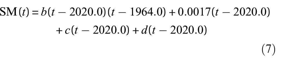
where
Figure 8 illustrates the observed and projected submergence at the Eugene Island 330 oil field area. The lowest scenario is based on a constant submergence rate of 15 mm/year, which comprises the average seafloor subsidence rate (12 mm/year) and the average regional SLR rate (2.6 mm/year) with respect to GOM20. Within the next 40 years, the lowest scenario will result in 0.6-m submergence; the intermediate-low scenario will result in approximately 0.8-m submergence; the intermediate-high scenario will result in approximately 1.0-m submergence; the highest scenario will result in approximately 1.3-m submergence. These projections provide a set of plausible trajectories for platform operators in the Eugene Island area to prepare for the future risks associated with WID damages. The highest scenario should be considered in planning critical and long-life offshore facilities in this area.
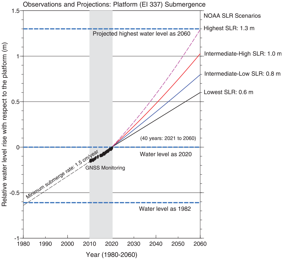
Observed (2010–2020) and projected (2021–2060) structure submergence at the DEV1 site. The projections for the future sea levels are based on the three global sea-levelrise (SLR) scenarios for the United States National Climate Assessment, National Oceanic and Atmospheric Administration (NOAA). 70
Conclusions and discussion
This article documents the details of the stand-alone GNSS monitoring methodology for offshore SHM. The stand-alone GNSS monitoring does not require installing any reference stations in the field and does not need to integrate any reference data in the data processing. Thus, the stand-alone GNSS monitoring method remarkably reduces field logistics costs and substantially improves the robustness of offshore SHM. According to this study, the RMS accuracy of daily positions is about 3–4 mm in the EW and NS directions and 7 mm in the vertical direction; the ongoing seafloor subsidence rate in the Eugene Island 330 oil field area is about 12 mm/year referred to the stable Gulf Coastal Plain, comprising approximately 10 mm/year anthropogenic subsidence and 2 mm/year natural subsidence; the ongoing structure submergence rate is approximately 15 mm/year; the Eugene Island 337-A platform has lost a minimum of 60-cm air gap during its 40-year history (1982–2021). A module for projecting future structure submergence is established through this study. According to this module, the structures in the Eugene Island 330 oil field area would submerge at least 60 cm in the next 40 years (2021–2060), likely between 0.8 and 1.0 m, but unlikely to exceed 1.3 m.
The methodology presented in this article has the potential for broad applications in other offshore regions where rigorous stable regional references are available. The geodesy research and surveying communities have installed over ten thousands of CORS around the globe since the early 1990s. 57 We are witnessing an exponential explosion in the number of CORS stations and the volume of continuous GNSS data. These long-term (e.g., >7 years) GNSS stations have accumulated fundamental datasets for establishing a series of regional or local-scale reference frames in the coastal regions around the globe. The author and his collaborators have established the stable Caribbean Reference Frame 2018 (CARIB18), 73 the stable North China Reference Frames (NChina16 and NChina20),74,75 the stable Northeast China Reference Frame, 76 and the stable South China Reference Frame 2020 (SChina20). 77 These regional reference frames will enable long-term offshore SHM within the Caribbean Sea, the Yellow Sea, the Bohai Bay, and the South China Sea, respectively. It is expected that this study will promote the applications of high-accuracy GNSS in offshore structures (e.g., platforms, wind turbines) health monitoring worldwide.
Footnotes
Acknowledgements
I acknowledge Mr. Randy L. Osborne at the Louisiana State University Center for Geoinformatics (http://c4g.lsu.edu) for providing GNSS data at DEV1 and DEV2, and Mr. Rick Ducote at Fieldwood Energy, LLC for providing site photos at DEV1. I appreciate Ms. Jennifer Welch for helping me contact the operator of the platform. I appreciate two reviewers for their very thoughtful comments. The onshore GPS used for this study are from UNAVCO (https://www.unavco.org), National Geodetic Survey (https://www.ngs.noaa.gov/CORS), and the Nevada Geodetic Laboratory (![]() ).
).
Declaration of conflicting interests
The author declared no potential conflicts of interest with respect to the research, authorship, and/or publication of this article.
Funding
The author received no financial support for the research, authorship, and/or publication of this article.