Improving sensitivity and coverage of structural health monitoring using bulk ultrasonic waves

Abstract

Practical ultrasonic structural health monitoring systems must be able to deal with temperature changes and some signal amplitude/phase drift over time; these issues have been investigated extensively with low-frequency-guided wave systems but much less work has been done on bulk wave systems operating in the megahertz frequency range. Temperature and signal drift compensation have been investigated on a thick copper block specimen instrumented with a lead zirconate titanate disc excited at a centre frequency of 2 MHz, both in the laboratory at ambient temperature and in an environmental chamber over multiple 20°C–70°C temperature cycles. It has been shown that the location-specific temperature compensation scheme originally developed for guided wave inspection significantly out-performs the conventional combined optimum baseline selection and baseline signal stretch method. The test setup was deliberately not optimised, and the signal amplitude and phase were shown to drift with time as the system was temperature cycled in the environmental chamber. It was shown that the ratio of successive back wall reflections at a given temperature was much more stable with time than the amplitude of a single reflection and that this ratio can be used to track changes in the reflection coefficient from the back wall with time. It was also shown that the location-specific temperature compensation method can be used to compensate for changes in the back wall reflection ratio with temperature. Clear changes in back wall reflection ratio were produced by the shadow effect of simulated damage in the form of 1-mm diameter flat-bottomed holes, and the signal-to-noise ratio was such that much smaller defects would be detectable.

Introduction

One of the major barriers to the wider replacement of periodic inspection (non-destructive testing (NDT)) by structural health monitoring (SHM) is that NDT often involves scanning a transducer over the area of structure to be inspected and this cannot be done with the fixed transducers used in SHM. This has led to great interest in ultrasonic-guided wave methods, since guided waves provide full volume coverage of large regions of structure from one^1,2 or a modest number^3–5 of transducer positions and so make large volume coverage economically feasible. ⁶ However, guided wave inspection typically operates in the tens to hundreds kilohertz (kHz) range and so is much less sensitive to small defects than megahertz (MHz) bulk ultrasonic wave inspection. The sensitivity of guided wave inspection can be significantly improved by comparing the current signal with a baseline obtained when the structure was defect-free or in a known defective condition. This requires compensation for signal changes caused by changes in the environmental conditions, notably temperature, and there has been a great deal of work on temperature compensation methods.^3–5,7–11 These compensation schemes now work very well, and sensitivity improvements in guided wave monitoring of a factor of ∼5 over the performance obtained in one-off NDT have been obtained in a blind trial. ¹ Recent work has further improved the compensation so that another factor of 5–10 improvement over that reported in the blind trial is possible. ¹²

The most common industrial application of guided wave monitoring is corrosion monitoring in pipes. Here, the best likely sensitivity with low-frequency (tens kHz) guided wave monitoring is of the order of 0.1% cross-sectional loss; ¹² in a typical 12-inch-diameter pipe with 10-mm wall thickness, this is equivalent to a defect of 3 mm (30% wall thickness) deep and ∼3 mm in circumferential extent, and in many cases, the sensitivity achieved at an acceptable false call rate will be less good than this. It is possible to use higher order guided wave modes ¹³ at a cost of greater signal complexity or to use a fundamental mode operating just below the cut-off frequency of the higher order modes. ¹⁴ These strategies give somewhat improved sensitivity at a cost of reduced volume coverage from each transducer position.

In thick structures where guided waves are not appropriate, or if significantly smaller defects need to be detected and/or if the likely defect location is well defined, it would be attractive to use an SHM system based on bulk ultrasonic wave testing in the MHz frequency range. Permanently installed bulk wave ultrasonic systems to monitor wall loss due to corrosion and erosion by simply measuring the arrival time of the back wall echo have been extensively applied,^15–18 and many of these systems compensate for changes in the speed of sound with temperature; there has also been some work on crack detection,^19–21 largely using the signal processing or imaging methods used in conventional inspection. If the methods to compensate the signals for changing environmental conditions developed for guided wave monitoring could be applied to the bulk wave case, it would be possible to use lower frequencies for crack detection than would typically be employed in one-off NDT; this would improve the economic case for the SHM system by increasing the volume covered by each transducer, ²² the sensitivity lost by operating at a lower frequency being recovered by tracking the signal with time.

This article investigates the use of the location-specific temperature compensation (LSTC) method that has proved very successful in guided wave monitoring^12,23 to the bulk wave case, and this new method is also compared with the well-known optimal baseline selection (OBS) technique. Laboratory tests on a thick copper block specimen are reported with simple defects in the form of flat-bottomed holes being introduced. The effect of repeated temperature cycling on the signals is then investigated, and a scheme for reducing the effect of signal drift with time is introduced.

Section ‘Test specimen and sequence of experiments’ describes the test specimen and test protocols. Section ‘Temperature compensation’ then describes the temperature compensation schemes used and the following section ‘Effect of temperature cycling with no damage growth’ shows how the signals with no change in damage state vary over repeated small and large temperature cycles. A method of compensating for signal drift with time is introduced in section ‘Use of back wall echo ratio to reduce influence of drift’, the resulting scatter in the processed signals with time in a constant damage state and the effect of damage introduction being reported in section ‘Results using back wall echo ratio’. This is followed by the conclusions of the article.

Test specimen and sequence of experiments

The test specimen shown in Figure 1 was a simple 120 × 120 × 50 mm³ copper block with a 0.25-mm thick, 13-mm diameter lead zirconate titanate (PZT) disc (PIC255, Physik Instrumente Ltd) operating in thickness mode bonded to the centre of the sample surface using an epoxy adhesive. To avoid reflections of surface waves from the edges of the small sample, the top surface was coated with a layer of ‘Stopaq’, a proprietary bitumen-like material (Seal Forlife Industries). This setup was originally designed to illustrate the benefits of reducing the test frequency in monitoring applications; ²² it is not suggested that it is an optimal design for long term monitoring, since stability problems with adhesive bondlines have commonly been reported^24,25 and the properties of the Stopaq coating are strongly temperature dependent. A USB oscilloscope and arbitrary waveform generator (Handyscope HS5) was used to generate the excitation signal and measure the reflections, which were amplified by 40 dB. In the initial laboratory tests, ²² the interest was in investigating the effect of frequency on the volume coverage so the excitation used was a relatively broadband three cycle, 2-MHz Hanning windowed toneburst and in Liu et al., ²² the response was band-pass filtered at different centre frequencies; a 1.5–2.5 MHz band-pass filter was used in the results reported here. In the new tests of this article, a five cycle, 2-MHz Hanning windowed excitation toneburst was employed and the received signals were passed through a digital 500-kHz high-pass filter to remove any low-frequency noise. A thermocouple was attached to the sample surface to measure the temperature during monitoring via a Pico TC-08 instrument.

Figure 1.

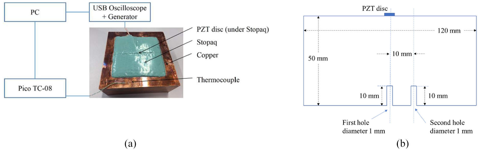
Specimen used: (a) photograph and (b) schematic diagram (not to scale).

Readings were collected in the laboratory at ∼10-min intervals over 6 days before the introduction of model defects in the form of flat-bottomed holes; the laboratory temperature varied by about 2.5°C over a daily cycle. Two holes were introduced sequentially, both being 1-mm diameter and 10-mm deep; the first was on-axis and the second was 10-mm off-axis, as shown in Figure 1(b). For the tests of Liu et al., ²² the second hole was extended to 2-mm diameter and 20-mm deep, but this extension is not relevant to this article. Readings were taken over 2 days following the introduction of each hole before further damage was introduced.

After the laboratory tests with defects were complete, the specimen was placed in an environmental chamber where it was subjected to 18 temperature cycles over a 20°C–70°C range. This enabled the operation of temperature compensation to be tested over a representative range and for the stability of the system to be investigated.

Temperature compensation

Two widely used methods for the temperature compensation of guided wave signals are baseline signal stretch (BSS) and OBS. While BSS requires only one baseline signal that is used as a reference to which any current measurement is compressed or stretched in time to minimise the residuals^4,8 in OBS, a set of baseline signals is stored so that the one deemed most similar to the specific current measurement is used for amplitude subtraction, often after also applying BSS on the selected baseline.^4,5 Both these techniques are, in principle, applicable to bulk wave as well as guided wave signals. There have also been several attempts to deal with the difficulty of temperature compensation on multi-mode-guided wave signals,^26,27 but this is not generally an issue in bulk wave ultrasound as it is relatively easy to obtain either a pure longitudinal or pure shear wave signal.

Recently, Mariani et al.^12,23 developed a new temperature compensation method denoted as LSTC that has been successfully applied to torsional-guided wave signals collected by permanently installed monitoring systems on pipes. ²³ Unlike the BSS, OBS and other previous methods that consider the whole signal in a single process, LSTC treats each point on the signal, corresponding to a particular location on the test structure, separately. The method comprises a calibration phase and a monitoring operation phase. In calibration, a set of baseline signals is acquired across the temperature range of interest, which is used to construct a calibration curve for each signal sample, that is, each point on the captured waveform. Each curve shows how the expected signal amplitude at each location in the absence of damage varies with temperature. In the monitoring operation phase, when a new measurement is acquired, at each point, the expected value at the relevant temperature obtained from the calibration curves is subtracted from the measurement itself. Thus, in the absence of damage, the expected value of the residual signal is zero. Further details are given in the Appendix and in Mariani et al. ²³ where it was also shown that the sequence of residuals obtained at any signal sample follows a normal distribution with approximately zero mean and with a standard deviation related to the incoherent noise level affecting the measurement. This makes it possible to apply change tracking algorithms such as the generalised likelihood ratio (GLR). ¹²

In this article, as in Mariani et al.,^12,23 the LSTC method was applied after first applying BSS compensation; this initial ‘global’ compensation corrects for wave speed changes with temperature and so ensures that the different signals are correctly ‘registered’, that is, a given sample point on each signal corresponds to the same location on the structure. While in the experiments reported here, the specimen temperature was measured and so could be used to identify the appropriate point on the calibration curves for each measurement, it is also possible to use the BSS factor as a surrogate temperature measurement.

Effect of temperature cycling with no damage growth

Laboratory tests around ambient temperature

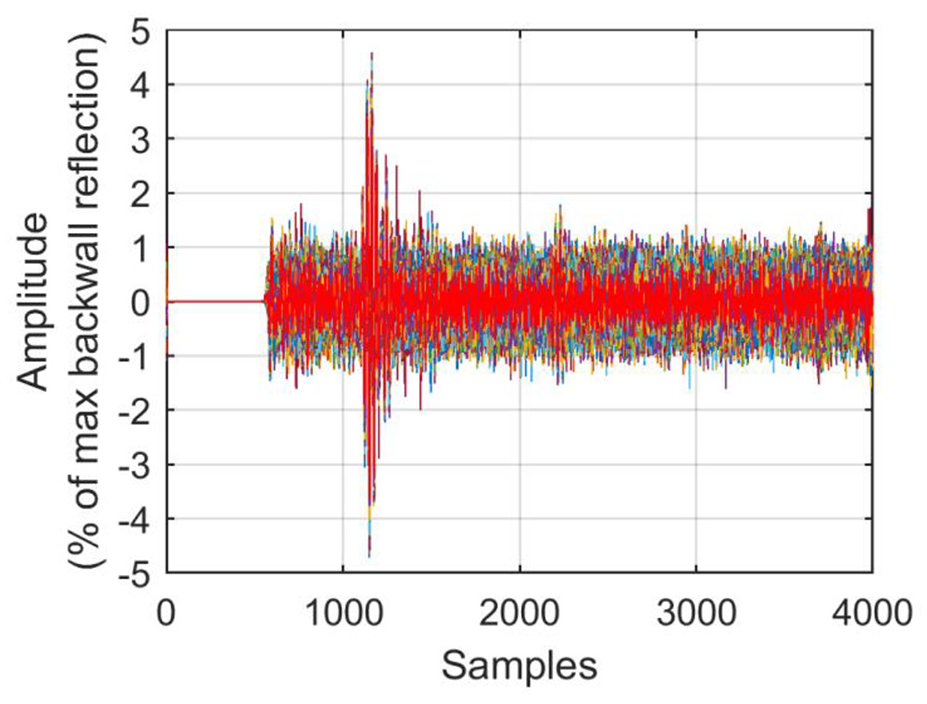
The initial tests on the sample before the introduction of damage were conducted in the laboratory over a period of 6 days. The temperature at each measurement point over the 6-day period is shown in Figure 2(a) and a typical A-scan signal showing longitudinal wave reflections from the back wall is presented in Figure 2(b), the amplitude being normalised to the maximum of the first-back wall reflection. The initial part of the A-scan signal corresponding to the excitation signal and amplifier recovery has been gated out, after which the first-back wall reflection and two reverberations can be seen; the 4000 samples in the A-scan correspond to a duration of 80 µs. The signal-to-noise ratio is poor as multiple small signals appear throughout the time trace; these are probably largely due to reverberations in the transducer assembly, though there is also some grain noise coming from the copper sample. No attempt was made to optimise the transducer or to identify the relative amplitudes of the sources of this coherent noise, as the purpose of this article is to investigate the ability of the monitoring scheme to subtract out the coherent noise; the noisy signal obtained here presents a more challenging case than an optimally designed system giving a very good signal to coherent noise ratio.

Figure 2.

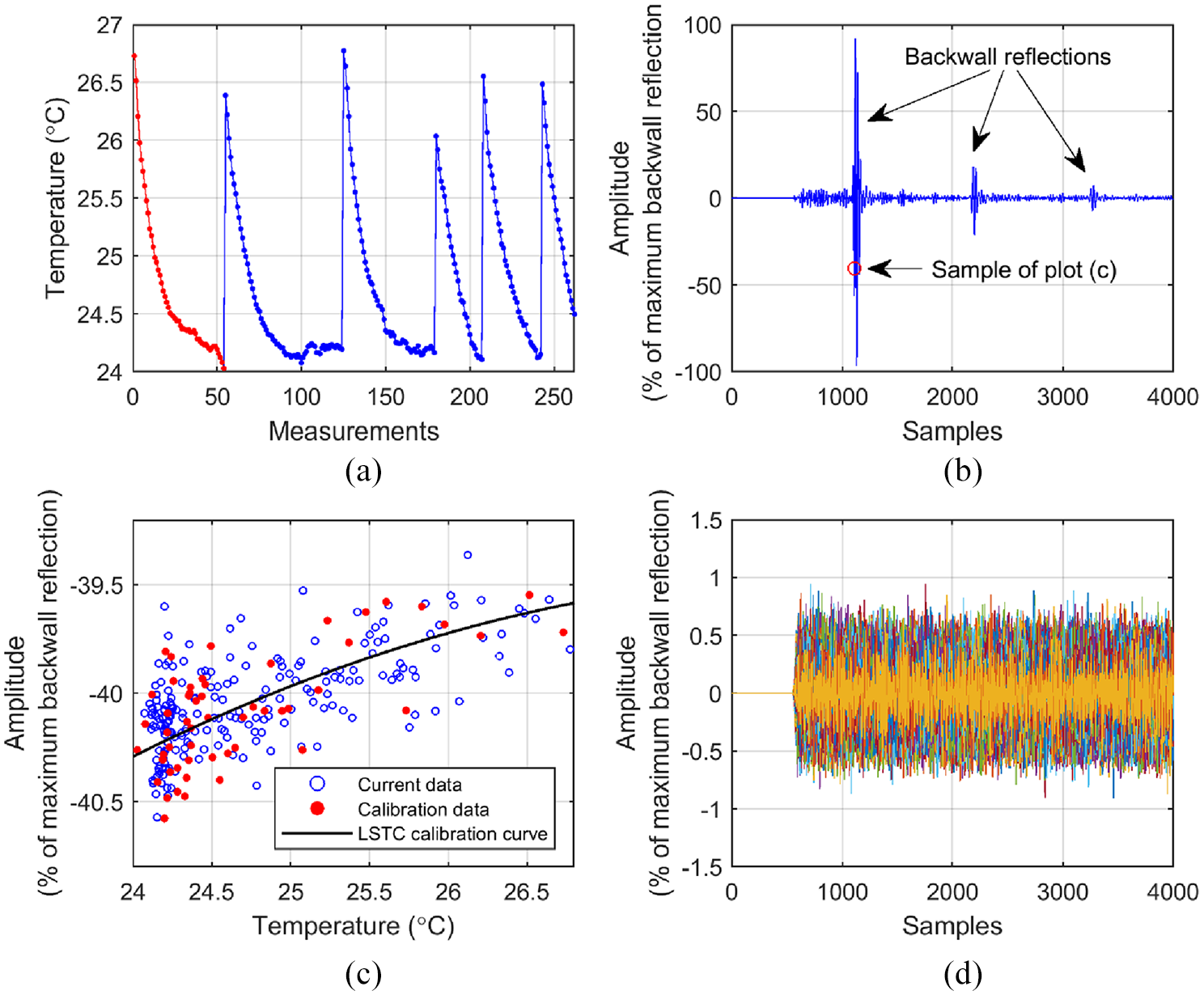
(a) Temperature at each measurement time in laboratory tests. Red – calibration data, blue –‘current’ data. (b) Typical A-scan signal normalised to maximum absolute envelope value. The 4000 samples correspond to an overall duration of 80 µs. (c) Typical LSTC calibration curve corresponding to sample 1111 marked with circle in (b). (d) Residual signals from each of the blue measurement points in (a).

The first day of data shown in red in Figure 2(a) was used as the calibration data set and Figure 2(c) shows an example LSTC calibration curve showing the signal amplitude as a function of temperature at sample 1111 marked in Figure 2(b). The LSTC calibration curve shown in black was fitted to the red points from the first, calibration, cycle using a second-order polynomial, while the blue points show the data from the subsequent cycles. The residual at each of the blue points was obtained by subtracting the value of the calibration curve at the relevant temperature from the amplitude of the blue point; the temperature range in these tests was only about 2.5°C so the signal changes are modest. Figure 2(d) shows the residual signal obtained from the LSTC compensation procedure at each of the blue measurement points of Figure 2(a). These superposed signals have zero mean (this would be expected as both signals are high-pass filtered, so any dc component is removed and the residual is formed by subtracting the two zero-mean signals) and a standard deviation of 0.20%. There is no apparent trend with position in the signal, showing that the subtraction to obtain the residual works well even when the original signal is large, for example, at the locations of the back wall echoes.

Tests in environmental chamber

After the experiments with damage introduction were concluded, the specimen was moved to an environmental chamber where it was subjected to 18 temperature cycles over ∼20°C–70°C, as shown in Figure 3(a), readings being taken at ∼70-s intervals; each cycle took about 20 h. There was a power interruption to the control system after about 16,000 readings when the temperature stayed at around its maximum value, as shown in Figure 3(a). Figure 3(b) shows the maximum amplitude of the first back wall echo as a function of measurement number. There is clear temperature dependence and drift with time; the maximum amplitude increases slightly with time over the first ∼4000 readings but then decreases gradually, the value after 18,000 readings being about 5% lower than the peak. The computed stretch factor in the BSS compensation shown in Figure 3(c) also varies with temperature and time; the variation with temperature is expected as the stretch factor accounts for the ultrasonic velocity change compared to the baseline (reading 5510 at 45°C) that changes roughly linearly with temperature difference, but at a given temperature, the stretch factor is expected to be constant with time, whereas Figure 3(c) shows that the minimum stretch value (corresponding to the minimum temperature and so highest velocity) changes from 0.9963 to 0.9956 over the 18 cycles.

Figure 3.

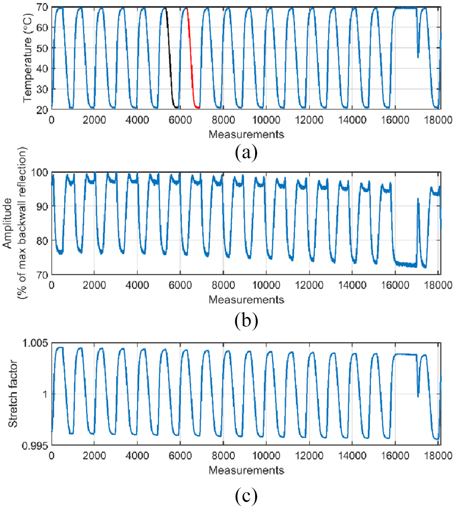
Tests in environmental chamber. (a) Temperature history over 18,131 measurements taken over ~15 days. Measurements marked in black and red are those used in Figure 5. (b) Maximum amplitude of first-back wall echo normalised to maximum value obtained in any test. (c) BSS factor relative to baseline (reading 5510 at 45°C).

This suggests that there is some distortion to the signal that changes the optimum value of stretch required to minimise the difference between the baseline and stretched current signals. Figure 4(a) shows the first-back wall echo from signals 1578 and 17,610, both of which were at 44.7°C, the shifts in both amplitude and phase being clear. Figure 4(b) shows the result of applying phase compensation, ²⁸ the main peaks now being correctly aligned, and Figure 4(c) shows the outcome of normalising the amplitude of the later signal to the earlier one taken as a baseline. The signals and their corresponding envelopes are almost identical in Figure 4(c) apart from a small phase shift in the tail of the signals, which can be seen more clearly in the zoomed plot of Figure 4(d). However, the back wall echo will be affected by damage, so normalising it to a baseline value will tend to obscure damage growth. Therefore, amplitude normalisation is unlikely to be an appropriate way to deal with the drift in amplitude with time, so another calibration method is required; this is addressed in the next section.

Figure 4.

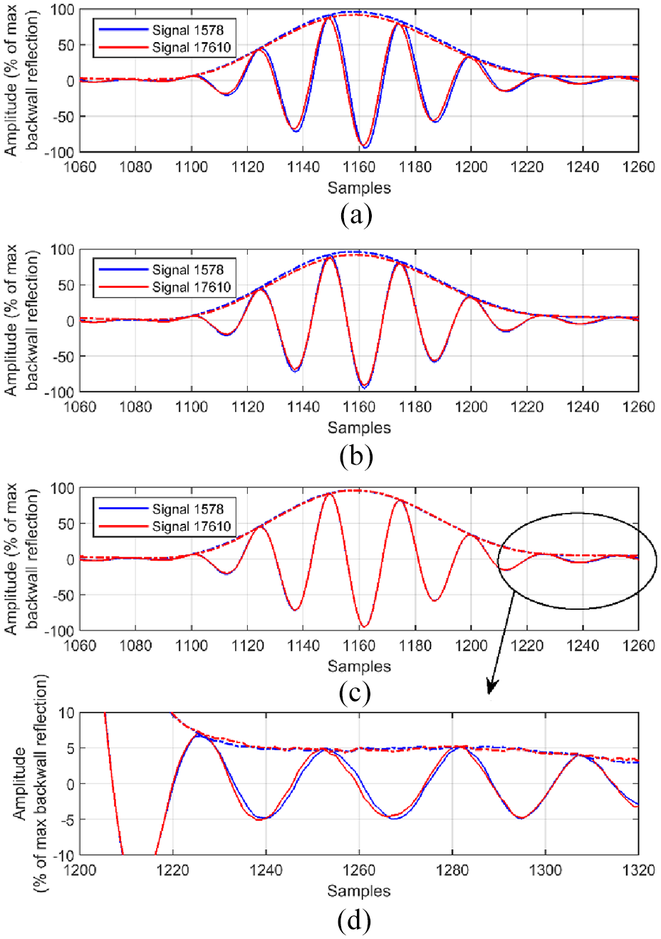
First-back wall echo in signals 1578 and 17,610, both of which were at 44.7°C: (a) as captured, (b) signals of (a) after phase compensation, (c) signals of (b) after amplitude normalisation and (d) zoom of tail region of (c).

The drift in amplitude and phase with time is probably caused by changes in the bonding of the PZT disc to the test piece and also in the damping provided by the Stopaq covering; this hypothesis is supported by the presence of changes in the reverberation seen immediately after the end of the excitation signal in the initial region gated out in Figure 2(b). As discussed above, the goal of the tests reported here was to explore issues in the application of SHM using bulk wave ultrasound, rather than to produce an optimised transduction system, so the cause of the drift was not investigated further.

The transduction system is relatively stable over a small number of cycles. For example, Figure 5(a) shows the sixth and seventh cycles that are plotted in black and red, respectively, in Figure 3(a). It is advantageous to take multiple baseline readings and ideally these will be spread fairly evenly across the range of temperatures. This is particularly important when the OBS and BSS compensation are used singly or in combination, ²⁹ and the work of Mariani and Cawley ¹² showed that multiple baselines, even taken around the same temperature, improve performance over a single reading. As an example, suppose that six clusters of five readings at ∼10°C intervals in the region of the points marked in blue in Figure 5(a) are used as baseline readings; this corresponds to a case where the temperature does not vary smoothly over the period when it is possible to take baselines. Figure 5(b) shows the residual signals obtained for each measurement in the second (red) temperature cycle of Figure 5(a) when using the LSTC temperature compensation method. The standard deviation of the residual signal is about 0.22% which is very similar to that obtained in Figure 2(d) when the temperature variation was only about 2.5°C, compared to the 50°C in this test. In contrast, Figure 5(c) shows the corresponding result when combined OBS and BSS temperature compensation was used with the same set of baseline readings. The peak-to-peak range of residual is now ∼9% compared to about 2% with LSTC in Figure 5(b), the peak residuals being around the location of the first back wall echo, as would be expected since the residual here is the difference between two large quantities. Figure 5(d) shows the variation of residual amplitude at sample number 1162 (the peak of the first back wall echo shown in Figure 4(a)) with measurement number using the two compensation methods. The LSTC residual is always small, whereas the OBS + BSS residual exhibits a sawtooth pattern, the residual being low when the temperature corresponding to the measurement number is close to that of one of the six calibration points. The jumps from negative to positive amplitudes in the residual occur when the optimum baseline selected switches from a baseline taken above the current reading temperature to one at a lower temperature or vice versa.

Figure 5.

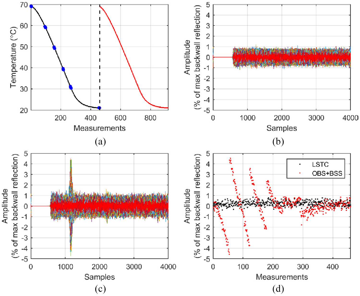
Temperature compensation over wide temperature range when transduction system is stable. (a) Sixth and seventh cycles of Figure 3(a) with measurement numbers set to zero at start of sixth cycle. Six clusters of five readings at ~10°C intervals in region of points marked in blue used as baseline readings. (b) Residual signals at each of points in red cycle of (a) using LSTC temperature compensation. (c) Corresponding plot to (b) but using OBS + BSS temperature compensation. (d) Variation in residual amplitude with measurement number at sample 1162 (maximum absolute value of back wall reflection in Figure 4(a)) using LSTC and OBS + BSS compensation; measurement number set to zero at the start of red cycle of (a).

These results demonstrate that the LSTC method is superior to the conventional OBS + BSS technique; this finding mirrors that seen with guided waves. ¹² Therefore, if a stable transduction system is designed, the LSTC method will provide very effective temperature compensation with bulk wave ultrasonic signals.

Use of back wall echo ratio to reduce influence of drift

Achenbach et al. ³⁰ proposed a self-calibration scheme for ultrasonic inspection. In a normal incidence configuration, such as that used in this article, it involves comparing successive reverberant reflections from the same reflector. Consider the setup of Figure 6 which is a schematic representation of the experimental arrangement of Figure 1. The transducer is shown separate from the top surface to emphasise the presence of an adhesive coupling layer, and the beam paths are shown non-normal to enable successive echoes to be distinguished. Interface 1 at the top surface is between the adhesive layer and the copper block, while interface 2 at the bottom surface is between the copper block and air. The first- and second-back wall echoes, $S_1$ and $S_2$ , are given by

$$S_1=P{T}_{1}A{R}_{2}A{T}_{1}P$$

(1)

$$S_2=P{T}_{1}A{R}_{2}A{R}_{1}A{R}_{2}A{T}_{1}P$$

(2)

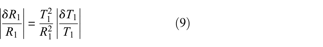
where P is the transduction sensitivity of the transducer (written as equal in transmit and receive, but this is not essential), A is the attenuation over the specimen thickness (including beam spread), R_i is the reflection coefficient from interface i, and T_i is the transmission coefficient for interface i. Then

$$\frac{S_2}{S_1}=R_1{R}_2{A}^2$$

(3)

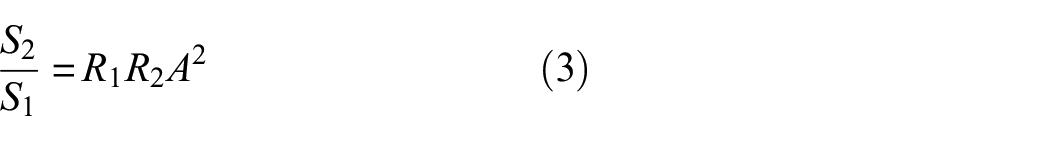
Since defects in the beam path will affect the back wall reflection, we are interested in tracking the value of R₂. The baseline value is R₂₀, so we have

$$R_1{A}^2=\frac{1}{R_{20}}{\left(\frac{S_2}{S_1}\right)}_0$$

(4)

where $(S_2/S_1{)}_0$ is the baseline back wall signal ratio. Hence, from equation (3), if R₁ is constant

$$\frac{R_2}{R_{20}}=\frac{\left(\frac{S_2}{S_1}\right)}{{\left(\frac{S_2}{S_1}\right)}_0}$$

(5)

We can, therefore, track changes in R₂ with time on the assumption that R₁ is constant. Unfortunately, R₁ will be affected by adhesive property changes and so may not be constant. The sum of the squares of the amplitude reflection and transmission coefficients is unity, so

$$R_1^2+T_1^2=1$$

(6)

Suppose the transmission coefficient decreases by $\delta T_1$ . Then

$$2R_1\delta R_1+2T_1\delta T_1=0$$

(7)

and considering a fractional change, $\delta T_1/T_1$ , which would give a corresponding reduction in ultrasonic amplitude for constant transducer excitation

$$R_1^2\frac{\delta R_1}{R_1}+T_1^2\frac{\delta T_1}{T_1}=0$$

(8)

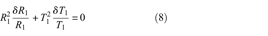
Hence

$$\left|\frac{\delta R_1}{R_1}\right|=\frac{T_1^2}{R_1^2}\left|\frac{\delta T_1}{T_1}\right|$$

(9)

There is a substantial acoustic impedance mismatch between copper (41.6 MRayl) and epoxy (∼3 MRayl), so the transmission coefficient across the interface is small relative to the reflection coefficient and the fractional change in the reflection coefficient from equation (9) is about one-third of the change in the transmission coefficient. Therefore, the ratio of equation (5) will be less affected by changes in the impedance of the epoxy layer than the absolute back wall reflection amplitudes, and the ratio is completely unaffected by changes in the piezoelectric properties or the excitation voltage. Therefore, we expect the ratio $S_2/S_1$ to be more stable with time than $S_1$ alone; this is tested in the next section.

Figure 6.

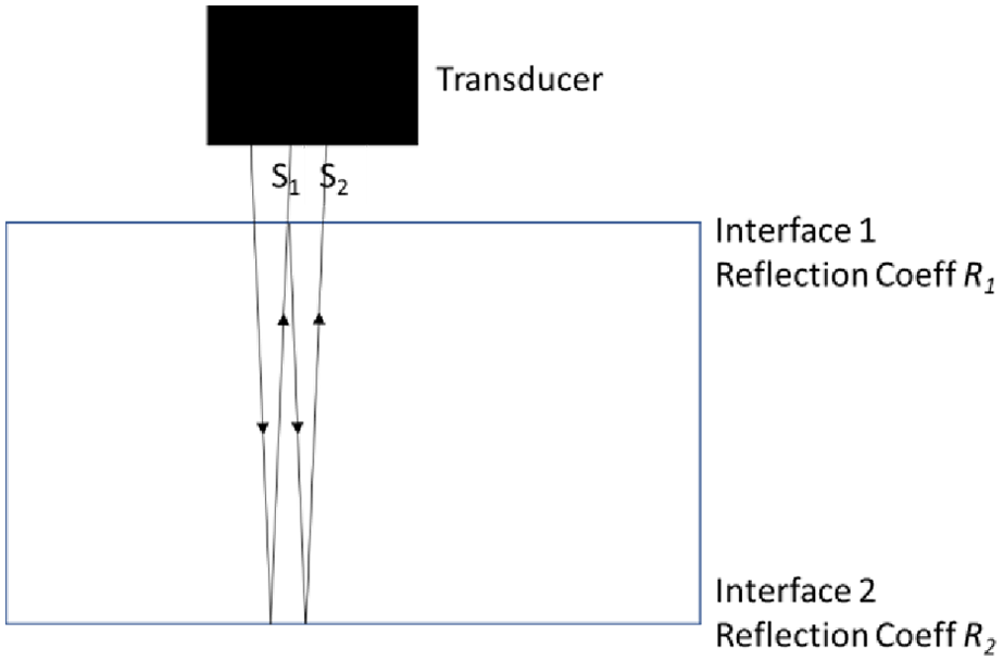
Schematic of wave paths for first- and second-back wall reflections

Results using back wall echo ratio

Figure 7 shows the outcome of LSTC temperature compensation on all measurements taken in the environmental chamber, using the six clusters of five readings in the region of points marked in blue in Figure 5(a) as baselines. The large excursions around sample 1150 correspond to the location of the first-back wall echo; it would be expected that uncompensated effects would have the largest effect at the location of the biggest reflector, since the residual signal at this location is the difference between two large quantities. Excluding the points in this region, the standard deviation is about 0.25% which is quite similar to the result of Figure 5(b). However, it is often of interest to detect defects close to the back surface or to see the shadowing effects on the back wall echo produced by defects in the body of the test piece, so obtaining a stable result at the location of the back wall echo is particularly important.

Figure 7.

Residual signals obtained with all 18,131 measurements using LSTC method with same baseline readings as in Figure 5(a).

Figure 8 shows the results obtained using the back wall ratio method in section ‘Use of back wall echo ratio to reduce influence of drift’. The variation of the amplitude of the first-back wall echo with time as the temperature was cycled was shown in Figure 3(b) and the second-back wall echo followed a similar pattern, as would be expected. Figure 8(a) shows the ratio of the second-back wall echo amplitude to that of the first over the full duration of the tests in the environmental chamber; there are significant oscillations corresponding to the temperature cycling. Figure 8(b) shows the LSTC calibration curve for the back wall echo ratio obtained from the ratio values of all the points in the first cycle of Figure 3(a), a fourth-order polynomial being used for the fit; a higher order was used than in Figure 2(c) as the temperature range covered was much larger. Figure 8(c) shows the result of applying LSTC compensation to the results of Figure 8(a) after the first, calibration, cycle. The ordinate of Figure 8(c) is the residual given by LSTC for the ‘current’ signal, expressed as a percentage of the baseline ratio. The moving average increases slightly up to about sample 8000 and then stabilises, in contrast to the back wall amplitude of Figure 3(b) that first increased and then decreased markedly with time. It is likely that the initial changes in the echo amplitudes and their ratio are caused by further curing of the adhesive as it is exposed to high temperatures for extended periods, the original cure having been at room temperature. This would cause irreversible acoustic impedance changes that will not be perfectly compensated by taking the ratio of successive back wall reflections, as explained in section ‘Use of back wall echo ratio to reduce influence of drift’; however, as indicated by equation (9), the ratio is less affected than the raw echo amplitude. The echo ratio is temperature-dependent, as seen in Figure 8(a) and (b), but the temperature dependence is consistent with time, so once the adhesive has stabilised, the LSTC compensated ratio is stable, as seen in Figure 8(c) from reading 8000 onwards. Therefore, the ratio method has compensated the downwards drift in the raw amplitudes shown in Figure 3(b). The standard deviation of the moving average line is about 0.22%.

Figure 8.

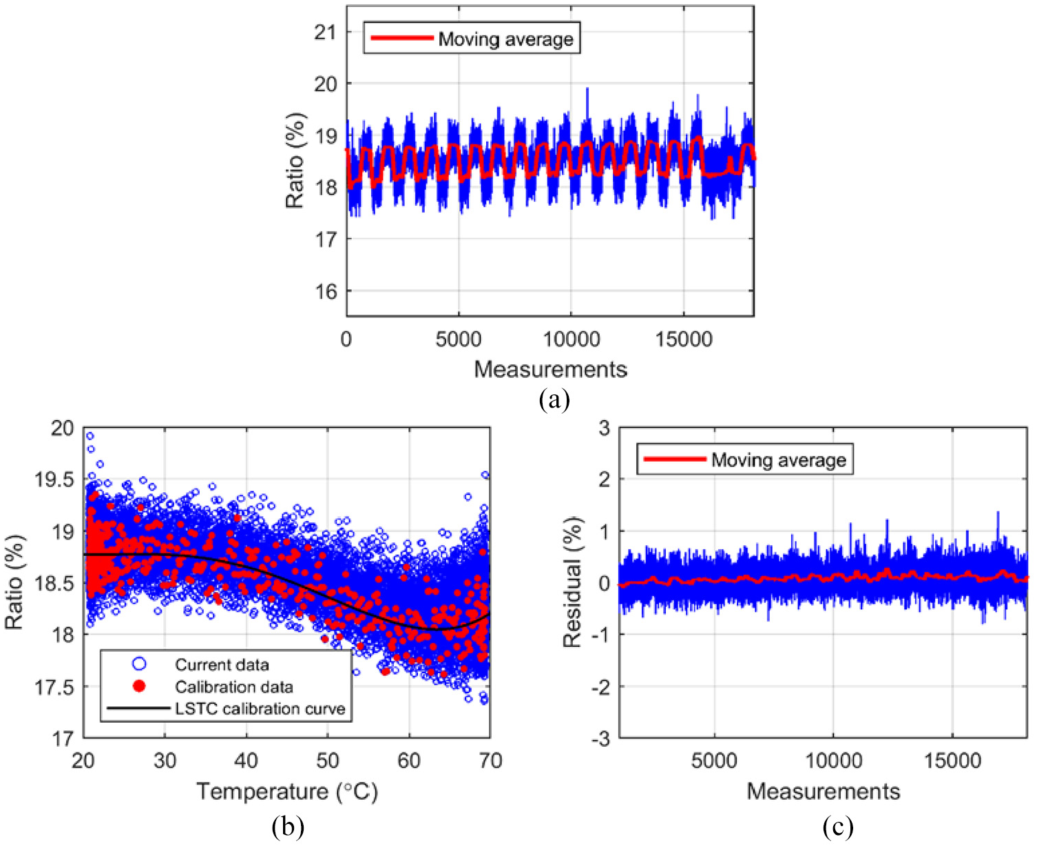
(a) Ratio of amplitude of second-back wall signal to first for all readings in environmental chamber, (b) LSTC calibration curve for ratio of first- to second-back wall reflection using first cycle of Figure 3(a) as baseline points and (c) residual back wall reflection ratio at each measurement from second cycle of Figure 3(a) onwards obtained using LSTC compensation and calibration curve of (b). Ordinate scale in (c) is percentage of baseline ratio.

Figure 9 shows the residual back wall ratio corresponding to that of Figure 8(c) obtained in the initial laboratory tests at ambient temperature as damage was introduced, the red lines showing the average residual ratio at each step. The standard deviation of the readings about the averages is 0.21% which encouragingly is very similar to that of Figure 8(c), indicating that there is no significant increase in scatter as more temperature compensation is required. The steps in the back wall echo ratio as first the on-axis hole of Figure 1(b) and then the off-axis hole was introduced can clearly be seen. The steps in the ratio are not equal, but this is to be expected as the shadowing effect of the defects on the back wall echo will be different for on- and off-axis holes. The ratio of the change in back wall echo ratio on introduction of the first hole to the standard deviation of the readings is ∼6 so it is clear that the defect is very reliably detected and it would be feasible to detect much smaller defects, provided frequent readings were obtained to remove the effects of the scatter via, for example, the GLR algorithm. ¹² Application of the algorithm is dependent on the scatter in the signal used being normally distributed. The degree to which the three clusters of residuals at each step of Figure 9 individually fit a normal distribution was checked by applying the Shapiro and Wilk ³¹ test which yielded p-values of 0.33, 0.83 and 0.56, thus, all comfortably passing the normality test at a 5% significance level, which requires the p-value to be greater than 0.05. Therefore, the echo ratio signals are appropriate for application of the GLR algorithm.

Figure 9.

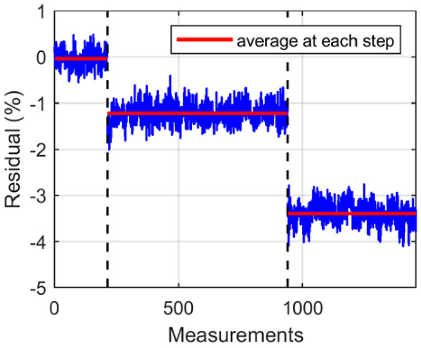
Residual back wall reflection ratio as damage grown in laboratory tests. First cycle of Figure 2(a) used as baseline; the first (undamaged) step includes each measurement from second cycle of Figure 2(a) onwards.

The results of Figure 8(c) show that the back wall echo ratio is much more stable than the back wall echo amplitude of Figure 3(b), even when values in Figure 3(b) are taken at a particular temperature (this can be seen from the changes in the maxima and minima with time). This suggests that the method can be used to address the problem of transducer drift, including changes in its bonding to the structure. Another problem that it will be important to address in some cases is corrosion causing changes in the roughness profile of the back wall and hence in the echo shape as well as its arrival time. ³² It has been shown that it is possible to obtain reliable thickness changes even in the presence of varying roughness profiles, ³³ but the changing nature of the back wall echo will make it impossible to detect small defects from changes in the back wall signal or the ratio of successive signals. Therefore, alternative compensation schemes will have to be devised.

Conclusion

Temperature and signal drift compensation of a bulk ultrasonic wave SHM system has been investigated. Tests have been carried out on a thick copper block specimen instrumented with a PZT disc excited at a centre frequency of 2 MHz both in the laboratory at ambient temperature and in an environmental chamber over multiple 20°C–70°C temperature cycles. It has been shown that the LSTC scheme originally developed for guided wave inspection works very well with bulk ultrasonic wave signals and significantly out-performs the conventional combined OBS and BSS method.

The test setup was deliberately not optimised, and the signal amplitude and phase were shown to drift with time as the system was temperature cycled in the environmental chamber. In the normal incidence setup used here, it was shown that the ratio of successive back wall reflections at a given temperature was much more stable with time than the amplitude of a single reflection, and that this ratio can be used to track changes in the reflection coefficient from the back wall with time. It was also shown that the LSTC method can be used to compensate for changes in the back wall reflection ratio with temperature. Clear changes in back wall reflection ratio were produced by the shadow effect of simulated damage in the form of 1-mm diameter flat-bottomed holes, and the signal-noise ratio was such that much smaller defects would be detectable. The LSTC residuals at each damage step were normally distributed about their mean value; this facilitates the application of change detection methods such as the GLR to track damage progression.