Change detection using the generalized likelihood ratio method to improve the sensitivity of guided wave structural health monitoring systems

Abstract

The transition from one-off ultrasound–based non-destructive testing systems to permanently installed monitoring techniques has the potential to significantly improve the defect detection sensitivity, since frequent measurements can be obtained and tracked with time. However, the measurements must be compensated for changing environmental and operational conditions, such as temperature, and careful analysis of measurements by highly skilled operators quickly becomes unfeasible as a large number of sensors acquiring signals frequently is installed on a plant. Recently, the authors have developed a location-specific temperature compensation method that uses a set of baseline measurements to remove temperature effects from the signals, thus producing “residual” signals on an unchanged structure that are essentially normally distributed with zero-mean and with standard deviation related to instrumentation noise. This enables the application of change detection techniques such as the generalized likelihood ratio method that can process sequences of residual signals searching for changes caused by damage. The defect detection performance offered by the generalized likelihood ratio when applied to guided wave signals adjusted either via the newly developed location-specific temperature compensation method or the widely used optimal baseline selection technique is investigated on a set of simulated measurements based on a set of experimental signals acquired by a permanently installed pipe monitoring system designed to monitor tens of meters of pipe from one location using the torsional, T(0,1), guided wave mode. The results presented here indicate that damage on the order of 0.1% cross section loss can reliably be detected with virtually zero false calls if the assumptions of the study are met, notably the absence of sensor drift with time. This represents a factor of 20–50 improvement over that typically achieved in one-off inspection and makes such monitoring systems very attractive. The method will also be applicable to bulk wave ultrasound signals.

Introduction

In the last decades, structural health monitoring (SHM) has been the subject of an enormous volume of research, although this has only resulted in a relatively small number of industrial applications. ¹ In contrast to non-destructive evaluation activities where an operator would typically deploy removable sensors and instrumentation to perform only one or a few measurements that will then be analyzed on a one-off basis, in SHM sensors and, sometimes, instrumentation are permanently installed on the structure, so that frequent measurements can be acquired, for example, daily. This enables comparisons to be drawn between the latest and earlier acquisitions to detect anomalies possibly caused by the occurrence of damage. In ultrasonic-based SHM, where either bulk waves or guided waves are used, “residuals” are typically obtained via amplitude subtraction between a “current” measurement (taken when the structure is at unknown health state) and a “baseline” signal (taken at an earlier time, when the structure was deemed defect-free), although the signals need first to be compensated for the effects of environmental and operational conditions, where the predominant factor is typically temperature.^2–6 Two widely used methods for temperature compensation are baseline signal stretch (BSS) and optimal baseline selection (OBS). While the former relies on storing only one baseline signal that is used as a reference to either compress or stretch in time any current measurement to minimize the residuals,^7,8 in OBS, a set of baseline signals is stored so that the one deemed most similar to the specific current measurement is used for amplitude subtraction, often after also applying BSS on the selected baseline.^7,9 In recent years, a number of other temperature compensation techniques have been developed. Fendzi et al. ¹⁰ proposed to divide a signal into time windows containing the arrival of a single wave mode and to apply temperature dependent amplitude and phase shift compensation factors within each window. In practice, this is complicated since the time windows would often contain multiple overlapping mode components. Zoubi and Mathews ¹¹ used a mode decomposition algorithm ¹² to decompose a set of baseline signals into possibly overlapped mode components and sought to determine mapping functions that describe the variations of each mode across the operating temperature range. Current measurements would then be compared to reconstructed baseline signals obtained from the predicted mode contributions at the measured temperatures. Douglass and Harley ¹³ presented a method based on dynamic time warping that maps each signal sample of the baseline measurement to a (possibly) different sample of the current signal, hence performing local stretches, although this can overfit the data, potentially masking defect reflections. Dao and Staszewski^14,15 avoided direct temperature compensation using a cointegration technique that already takes into account environmental changes and looks for departures from a stationary residual signal to detect the occurrence of damage.

Probably, the most successful applications of ultrasonic systems in SHM are in the oil and gas field, where permanently installed localized thickness monitoring systems have already been installed at ∼150 sites worldwide,^16,17 systems to monitor the growth of known cracks have been recently deployed,^18,19 and long-range devices using mostly torsional guided waves are routinely used to monitor tens of meters of pipe from a single transducer location for corrosion growth.^20–23 These systems are already producing a very large amount of data, which will only keep increasing as more devices are installed in the future. Therefore, the industry needs reliable algorithms that allow either full automatic evaluation of incoming signals or at least pre-screening in order to reduce the stream of data to be seen by human operators.

Recently, the authors of this article have developed a novel temperature compensation method denoted location-specific temperature compensation (LSTC)^6,24 that has been successfully applied to torsional guided wave signals collected by permanently installed monitoring systems installed on pipes, ²⁵ and, in principle, it can also be used on measurements acquired on other structures and using other guided wave modes or standard bulk waves. Mariani et al. ⁶ also showed that the sequence of residuals output by LSTC at any signal sample, that is, at each point on the captured waveform, follows a normal distribution with mean close to zero and standard deviation related to the incoherent noise level affecting the measurement.

If ultrasonic measurements can be processed and reduced to sequences of normally distributed samples, one can shift the paradigm of damage detection using ultrasound into a task of change detection as typically performed in the statistical process control (SPC) field. In the past century, researchers in SPC have produced a number of methods for quality control of manufacturing processes that involve the analysis of monitored parameters (e.g. temperature, pressure, and humidity) which are typically assumed to follow normal distributions.^26,27 The first and still widely used method is the Shewhart control chart. ²⁸ The first step in constructing a Shewhart chart is to determine the mean and standard deviation of the monitored parameter when that is in-control (i.e. when the controlled product is non-defective, so that measured variations are solely due to the effects of noise). Upper and lower limits are then set such that when a reading is outside the two limits, the process is deemed out-of-control (i.e. some undesired or unpredicted change has occurred). The method works well when the goal is to detect large changes, but it is not as effective when targeting subtler changes because it only makes use of the last available reading, hence ignoring the information available in the whole string of measurements. ²⁹ In contrast, another widely used method called cumulative sum (CUSUM) enables the detection of much smaller changes by making use of the information contained in all the past readings. ³⁰ However, this method requires the expected change to be specified in advance, and the detection performance worsens for changes other than the expected one. Starting from the 1990s, increasing computer power has resulted in increased attention from SPC researchers to the generalized likelihood ratio (GLR) change-point approach, which was first proposed by Lorden ³¹ in 1971. Although the GLR is rather computationally intensive, it offers the key advantage that it does not require the extent of change to be specified in advance.

This class of methods is potentially very attractive for the processing of ultrasonic SHM signals, whether using bulk or guided waves. In this article, an automated damage detection framework based on the GLR method is proposed, and the performance offered when used to analyze signals acquired for long-range screening of pipes is evaluated. The article is organized as follows. Section “Change detection algorithm for SHM” introduces the GLR method and the proposed framework for its application in SHM. Section “Multiple tests at fixed temperature” presents a study performed on simulated data sets to investigate the defect detection performance offered by GLR when multiple ultrasonic measurements are acquired at a fixed temperature. Section “Multiple tests at varying temperature” extends the results of the study to the more practical scenario of testing performed over a significant operating temperature range. Section “Experimental validation” describes the experimental tests that were used throughout the article to guide the formation of the simulated data sets and which are used to validate some of the results obtained from the numerical study. The main conclusions are then given in the final section “Conclusion.”

Change detection algorithm for SHM

Two key assumptions are made in defining the change detection problem, the first being that, at each signal sample, the sequence of residuals obtained after applying the LSTC method follows a normal distribution N(μ₀, σ²), where μ₀ tends to zero as more baseline measurements are used to calibrate the compensation method while the standard deviation σ is dictated by the level of incoherent noise affecting the measurements. The effectiveness of the LSTC method to produce residuals that are normally distributed will be tested in section “Investigation on the calibration curves produced by LSTC” for the data set used in this study. The second assumption is that if at some point in time damage was to occur somewhere in the test structure, that would produce a change in the residual signals coming from each point affected by the damage such that the residuals after the change will also follow a normal distribution N(μ₁, σ²), in this case characterized by an unknown shift in mean v = μ₁ − μ₀, that will be at least loosely related to the severity of damage, and an unmodified standard deviation σ. The latter assumption is justified by the fact that the level of random noise affecting the measurements after formation or growth of damage is still due to instrumentation noise that is independent of any change occurring in the structural geometry. By extension, further damage growth would induce further shifts in the mean and would still not affect the standard deviation. These assumptions are expected to hold as long as the sensors used for inspection are “stable” over time, that is, their frequency response functions may vary with temperature, but remain unchanged with time.

Under these assumptions, the GLR method has been shown to be the optimal monitoring scheme for change detection (which in this context is equivalent to defect detection) under appropriate definitions of statistical optimality. ³² The general framework in which the GLR method operates is based upon likelihood techniques, which have been already explored in a guided wave SHM context, for example, by Flynn et al., ³³ although via a rather different formulation and application, namely, damage localization in plate-like structures from the analysis of a single measurement. To derive the GLR formulation for change detection, it is essential to introduce the concept of the logarithm of the likelihood ratio, ²⁷ often referred to as the log-likelihood ratio. In a simple hypothesis test, supposing we have a single observation Y of a random variable y and we need to determine whether y belongs to a distribution θ₀ (the null hypothesis) or a distribution θ₁ (the alternative hypothesis), the log-likelihood ratio is defined by

$$s\left(Y\right)=\ln \frac{p_{{\theta }_1}\left(Y\right)}{p_{{\theta }_0}\left(Y\right)}$$

(1)

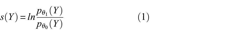
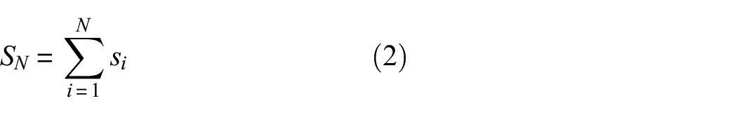
where p(·) is the probability density function operator (also referred to as relative likelihood). If we had to make a decision solely based on the available single observation, for s negative, we would accept the null hypothesis, whereas for s positive, we would reject the null hypothesis and so accept the alternative one. When, instead, a set of N observations is available, the optimal test would be the sequential probability ratio test (SPRT), ³⁴ which is defined as the sum of consecutive log-likelihood ratios

$$S_N=\sum _{i=1}^N{s}_i$$

(2)

In this case, an appropriate threshold h can be set, so that when

$$S_N\ge h$$

(3)

the alternative hypothesis is accepted. Note that in SPRT, the assumption is that the whole sequence of observations is drawn either from θ₀ or from θ₁. In contrast, in a change detection scenario, we have a sequence of N observations that initially are drawn from θ₀ and the goal is to determine whether the observations acquired after a certain point in time (the change point) are drawn from θ₁. Note that the possibility that the change point had already occurred before the first available observation is not excluded; these are the circumstances under which the CUSUM algorithm operates. ³⁰ When set to operate under appropriate parameters, the CUSUM algorithm can be interpreted as a set of N parallel SPRTs, one of which is activated at each possible change time i = 1,…, N. ³¹ Change is flagged if any of these SPRTs exceed the set threshold h.

When θ₁ is unknown, the GLR algorithm can be derived from the CUSUM method by substituting the unknown distribution parameters with their maximum likelihood values as first laid out by Lorden. ³¹ This actually corresponds to a double maximization, since both the change point and the possible set of parameters defining θ₁ need to be replaced by their maximum likelihood estimates based on the available observations, so that the GLR test score at the Nth observation is defined as

$$g_N=\underset{1\le j\le N}{max}\underset{{\theta }_1}{\sup }{S}_j^N\left({\theta }_1\right)$$

(4)

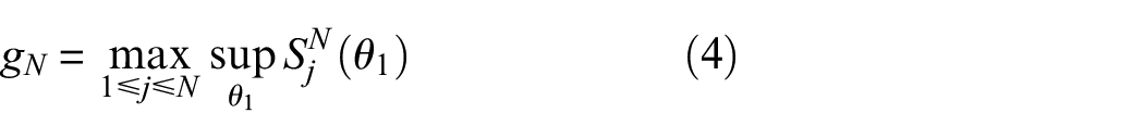
As in the previous analysis, a change is detected if g_N exceeds a set threshold h. For the case at hand, where both θ₀ and θ₁ are normal distributions with mean µ₀ and µ₁, respectively, and σ is unchanged, the double maximization of equation (4) is possible and the g_N formula assumes the following form, the derivation of which can be found, for example, in Basseville and Nikiforov ²⁷

$$g_N=\frac{1}{2{\sigma }^2}\underset{1\le j\le N}{max}\frac{1}{N-j+1}{\left[\sum _{i=j}^N(Y_i-{\mu }_0)\right]}^2$$

(5)

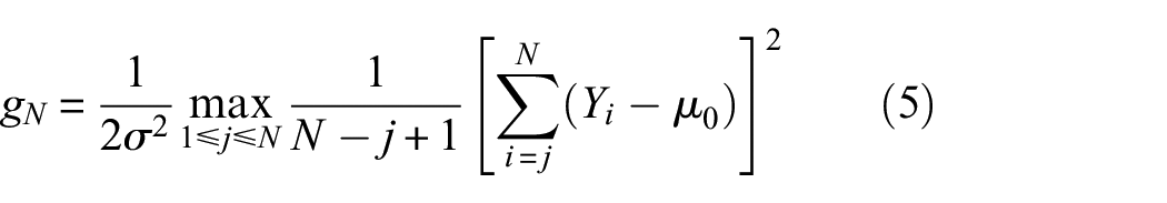
where the change point estimate is the observation j_cp that maximizes equation (5) and the change magnitude estimate is

$$\nu =|{\mu }_1-{\mu }_0|=\frac{1}{N-j_{\mathrm{cp}}+1}\sum _{i=j_{\mathrm{cp}}}^N|Y_i-{\mu }_0|$$

(6)

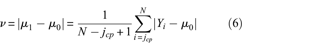
In the SHM framework proposed in this article, Y_i is the amplitude of the residual produced by LSTC at a given signal sample at measurement i, µ₀ is set to zero (although it will be only close to zero since LSTC uses a finite number of baseline signals; hence, the temperature compensation will not be exact), and the level σ of incoherent noise affecting the measurements is estimated from the baseline signals, for example, using the procedure illustrated in section “Investigation on the calibration curves produced by LSTC.” Every time a new measurement is acquired and compensated via LSTC, an updated GLR test score is computed at each signal sample via equation (5), and it is compared to the set threshold, so that a defect is called at the location(s) corresponding to any signal samples at which the threshold is exceeded.

Multiple tests at fixed temperature

Simulation of undamaged signals and application of LSTC or OBS to generate residuals

A Monte Carlo analysis based on numerically generated data was performed to investigate the improvement in sensitivity offered by the GLR method when the information contained in multiple tests is treated as a whole rather than independently. Without loss of generality, for the study described in this section, we assume that the true (noise-less) underlying signal before change is constant and equal to zero, so that each (simulated) measurement produces a normally distributed signal with zero-mean and standard deviation σ. Note that the underlying signal radio frequency (RF) shape is exploited by the BSS method to compute the stretching factor required to compensate for the changing wave speed at various temperatures, but since in this section we investigate the case of fixed temperature, time-stretching compensation is not needed. When analyzing ultrasonic measurements, it is generally advantageous to filter out frequency components outside a band around the center frequency of the excited signal. Therefore, a specific central frequency had to be chosen to produce the numerical data set, and this was taken as that used in the experimental data set described in section “Experimental validation,” that is, 23.5 kHz sampled at a frequency of 200 kHz. Therefore, each numerically simulated measurement was produced by (1) generating an N(0,1) distributed random sequence of a set number of samples, then (2) band-pass filtering the sequence via a Butterworth filter of order 4 and cut-off frequencies of 20 and 27 kHz, and (3) multiplying the filtered sequence by an appropriate factor to restore a standard deviation σ = 1, this being needed since the filtering process also reduces the signal energy. For example, Figure 1(a) plots five such measurements with a set length of 400 samples (i.e. 2 ms at the chosen sampling frequency), while the blue plots in Figure 1(b) and (c) show the first of those signals in the time and frequency domains, respectively. Note that the various measurements are independent from each other; thus, each sequence of values obtained by selecting a fixed location in the fast-time (i.e. time base of ultrasonic wave signal arrivals) and then being laid out in the slow-time direction (i.e. across multiple measurements) is still an N(0,1) distributed independent random sequence. For example, Figure 1(d) shows the sequence of amplitudes recorded at the first sample of 500 different measurements (the first five of these 500 measurements being those shown in Figure 1(a)), whose frequency content plotted in Figure 1(e) displays its broadband nature.

Figure 1.

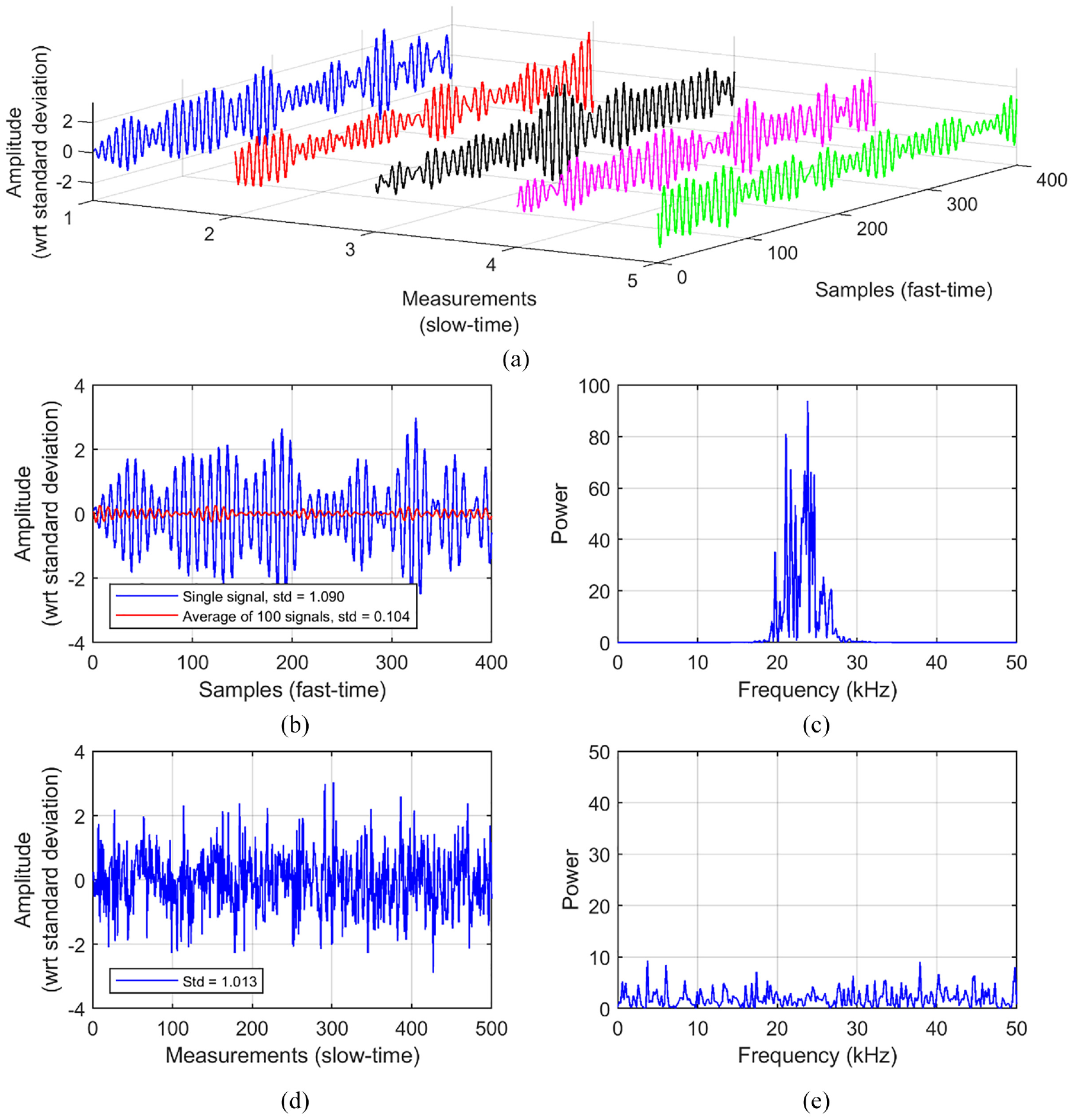
(a) Example of generation of five (undamaged) measurements. (b) Fast-time trace of the first measurement in (a) (blue) and average of 100 measurements obtained as in (a), including the five shown (red). (c) Power spectrum of blue trace in (b). (d) Slow-time trace obtained by tracking the first sample of 500 measurements generated as those in (a), including those five. (e) Power spectrum of trace in (d).

In this scenario of fixed measurement temperature, calibrating the LSTC method reduces to taking averages at each signal sample across the baseline signals. Central limit theory, by means of the Bienaymé formula, ³⁵ shows that the mean of n observations drawn from a normal distribution with mean μ and standard deviation σ also follows a normal distribution with mean μ and reduced standard deviation ${\sigma }_n=\sigma /\sqrt{n}$ . For example, the red plot in Figure 1(b) shows the average of 100 measurements, which is centered around zero and has an expected standard deviation of ${\sigma }_{n=100}=1/\sqrt{100}=0.1$ . This uncertainty in the determination of the true underlying signal (i.e. constant at zero in this case but generally an RF signal comprising coherent noise superposed on a sequence of waves reflected from real features in the test structure) will limit the defect sensitivity offered by GLR method, given that the probability of false alarm (PFA) needs to be kept very low in an SHM framework, as discussed, for example, by Cawley. ¹ In fact, if the apparent underlying value predicted by the LSTC calibration phase at any specific signal sample is on average 0.1 standard deviations away offset from its actual true value, the residuals computed in the undamaged structure will also be offset, on average, by 0.1 standard deviations away from zero, since they will actually be distributed around their unknown true value rather than the calibration value. Clearly, this uncertainty sets a lower limit on the size of the reflection from a defect that can be reliably called without possibly including a number of false alarms (FAs). It follows that, on average, the larger the available number N_BAS of baseline signals, the better the sensitivity that can be achieved. Only an infinite number of baselines would allow the LSTC method to be perfectly calibrated on the actual true underlying signal, and this scenario would represent the upper limit of sensitivity that can be offered when analyzing a given set of current signals. Since the true underlying signal is known in this study, the performance offered by this best-case scenario is also investigated and the results obtained in these conditions are denoted LSTC_∞. Similarly, the term ${\mathrm{LSTC}}_{N_{\mathrm{BAS}}}$ will indicate the number of baselines used to obtain the results shown in this article.

It is also of interest to compare the performance that would be obtained when the signals are compensated via OBS rather than LSTC, since the former has found wide application in SHM. In order to set the OBS method, a criterion needs to be defined that characterizes the similarity between any signal in the baseline data set $s_n(t)$ and the current measurement $s(t)$ , thus selecting the best match among the N_BAS baselines. A sensible criterion is to minimize the mean square deviation, ⁷ as

$$n_{\mathrm{OBS}}=\underset{n}{\arg \min }\left\{\underset{t1}{\overset{t2}{\int }}{[s\left(t\right)-s_n\left(t\right)]}^2\mathrm{dt}\right\}$$

(7)

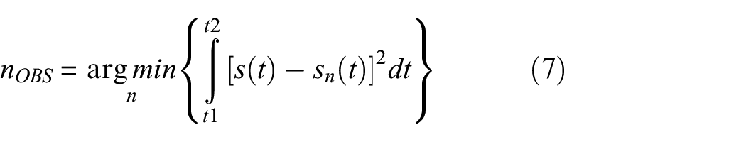
which is adopted throughout this study. When measurements are acquired at various temperatures, equation (7) typically results in selecting n_OBS among a restricted set of baseline signals taken at a similar temperature as the current measurement, since those RF shapes will be the most similar to the latter. Among those, the one chosen will be that in which, on average, the incoherent noise best matches that in the current signal. For example, referring again to Figure 1(a), but supposing this time that the first four signals represent the baseline set and the fifth signal is the current measurement, the application of equation (7) results in the selection of the second baseline measurement as n_OBS. The other available three baseline signals are discarded and not used in the compensation process of the considered current measurement. This highlights a key difference between the OBS and LSTC compensation methods, since the latter, in contrast, makes use of all the information contained in the baseline set. In addition, when the current signal also contains a reflection from a defect, OBS might tend to mask it by possibly selecting as n_OBS a baseline signal whose incoherent noise has a similar shape to the defect reflection. For both of these reasons, the performance offered by OBS is somewhat worse than that offered by LSTC, as shown in the following. Consistently with the assumed nomenclature, ${\mathrm{OBS}}_{N_{\mathrm{BAS}}}$ will be used to indicate the results obtained when using OBS with a certain number N_BAS of signals available in the baseline set.

Simulation of damage and application of GLR method

Regardless of the exact RF shape of the reflections from a defect, the sensitivity is almost entirely dictated by its highest absolute value, which is expected to produce the highest GLR test score. Throughout this study, defect signatures have been simulated by considering damage producing uniform frequency response ³⁶ (i.e. such that the shape of the reflected signal is the same as that of the input signal). Such a signature can be scaled to obtain the desired peak amplitude of its envelope, that is set relative to the standard deviation of incoherent noise affecting the measurements, and can then be added to an undamaged signal at the desired location by superposition, following a procedure validated in Heinlein et al. ³⁷ The experimental setting described in section “Experimental validation” was used to guide the choice of the input signal and hence of the defect reflection, this being an eight-cycle, 23.5-kHz Hanning-windowed toneburst.

Figure 2(a), (c) and (e) illustrates the generation of a current signal including a defect reflection whose peak amplitude equals the standard deviation of the incoherent noise. Here, the defect reflection shown in Figure 2(a) is added to the undamaged signal of Figure 2(c) to obtain the signal of Figure 2(e). This signal is also directly equal to the residual signal that would be obtained using LSTC_∞, since that would be obtained by subtracting zero from every sample (since the true underlying signal in this study is constant at zero). By contrast, as explained in the previous section, when a finite number of baselines is used to estimate the true underlying signal, there will be an estimation error such that the residuals will tend to be slightly offset from those of Figure 2(e) (the lower N_BAS, the larger the error, on average). Furthermore, depending on the degree of alignment between the phases of the defect signature and of the undamaged signal at the defect location, the amplitude of the former after superposition can appear magnified or reduced, so its detection when buried in measurement noise can be more or less challenging. For example, the specific case of Figure 2(a) and (c) is that of the noise and defect time traces being mostly out-of-phase, and the presence of the defect reflection in Figure 2(e) cannot easily be detected. Overall, it is clear that it would not be possible to detect defects at this size without also including a large number of FAs when only considering a single time trace at a time.

Figure 2.

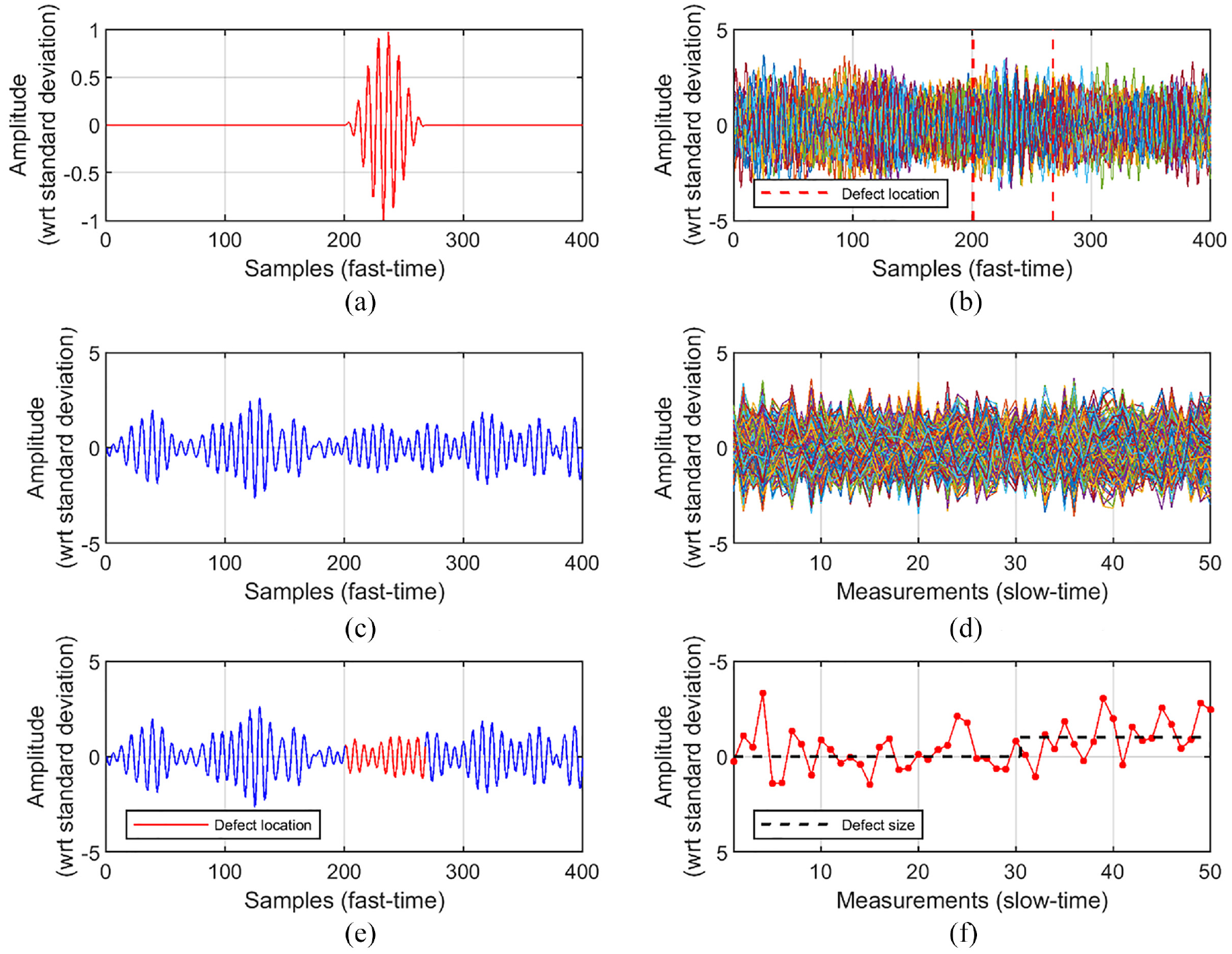
(a) Defect reflection whose peak amplitude equals the standard deviation of incoherent noise (note that the vertical scale of this plot is different than that of the others). (c) Undamaged signal generated as those discussed in Figure 1. (e) Defective signal obtained by superposition of those shown in (a) and (c). (b) 50 current measurements superposed in the fast-time direction, the latest 20 of which include the defect reflection plotted in (a). Red dashed lines indicate location of defect signal. (d) Contains the same data set as in (b) but plots the signals at each sample number (fast-time) as a function of measurement number (slow-time). (f) Slow-time trend measured at the defect peak (sample 233). The introduction of the defect in (a) after measurement 30 induces a change of normal distribution from N(0,1) to N(1,1).

Figure 2(b), (d) and (f) extends this scenario by supposing that 50 current measurements are acquired, the first 30 being undamaged and the latest 20 including the defect shown in Figure 2(a), as shown in Figure 2(e). The presence of the defect across the slow-time direction is illustrated via the black dashed plot of Figure 2(f). Figure 2(b) shows the 50 signals superposed on each other in the fast-time direction, while Figure 2(d) plots the signals at each sample number (fast-time) as a function of measurement number (slow-time). By visual inspection of the fast-time signals, it appears rather complicated to detect the defect signatures existing in the 20 defective measurements, although it can be noticed that the RF shape shows some degree of coherence at the defect location, as expected. It appears even more challenging to notice any particular trend in the slow-time sequences of Figure 2(d). Indeed, even by careful inspection of the trend measured at the defect peak (sample 233), shown in Figure 2(f), it is not trivial to detect the known deviation from 0 to 1 (on average) occurring after the 30th measurement.

Once the GLR method is applied to the LSTC_∞ compensated sequences of residuals shown in Figure 2(d) (residuals that, as already explained, are identical to the signals themselves in this considered scenario), the presence of the defect reflection is more easily identified. The results are given in Figure 3(a) and (b) in the fast-time and slow-time directions, respectively. While Figure 3(a) plots the GLR test scores obtained at each sample when treating the entire 50-point long sequences, Figure 3(b) also shows the scores that would have been achieved at each intermediate step, that is, when using the signals from the first up to the specific measurement number. Note that in the latter plot, for clarity, only the test score obtained at the defect peak (sample 233) and those obtained away from the defect location (samples depicted in blue in Figure 3(a)) are shown. The two plots also indicate a possible choice of threshold value, set to 8, such that a defect would be automatically called when a GLR test score at any location exceeds it. In fact, in this specific instance and by setting this threshold, the GLR method would have called this defect at measurement 45, when the threshold was first crossed, that is, after 15 measurements acquired since the defect was actually introduced. Clearly, when choosing a threshold, one needs to find a suitable tradeoff between (1) the expected level of PFA that is acceptable, (2) the minimum size of defect that needs to be detected with some prescribed probability of detection (PD), and (3) how many measurements one is willing to wait, at most, before a defect of such a size is called. In the next section, a framework that can be used to identify an appropriate threshold by considering those three requirements is presented.

Figure 3.

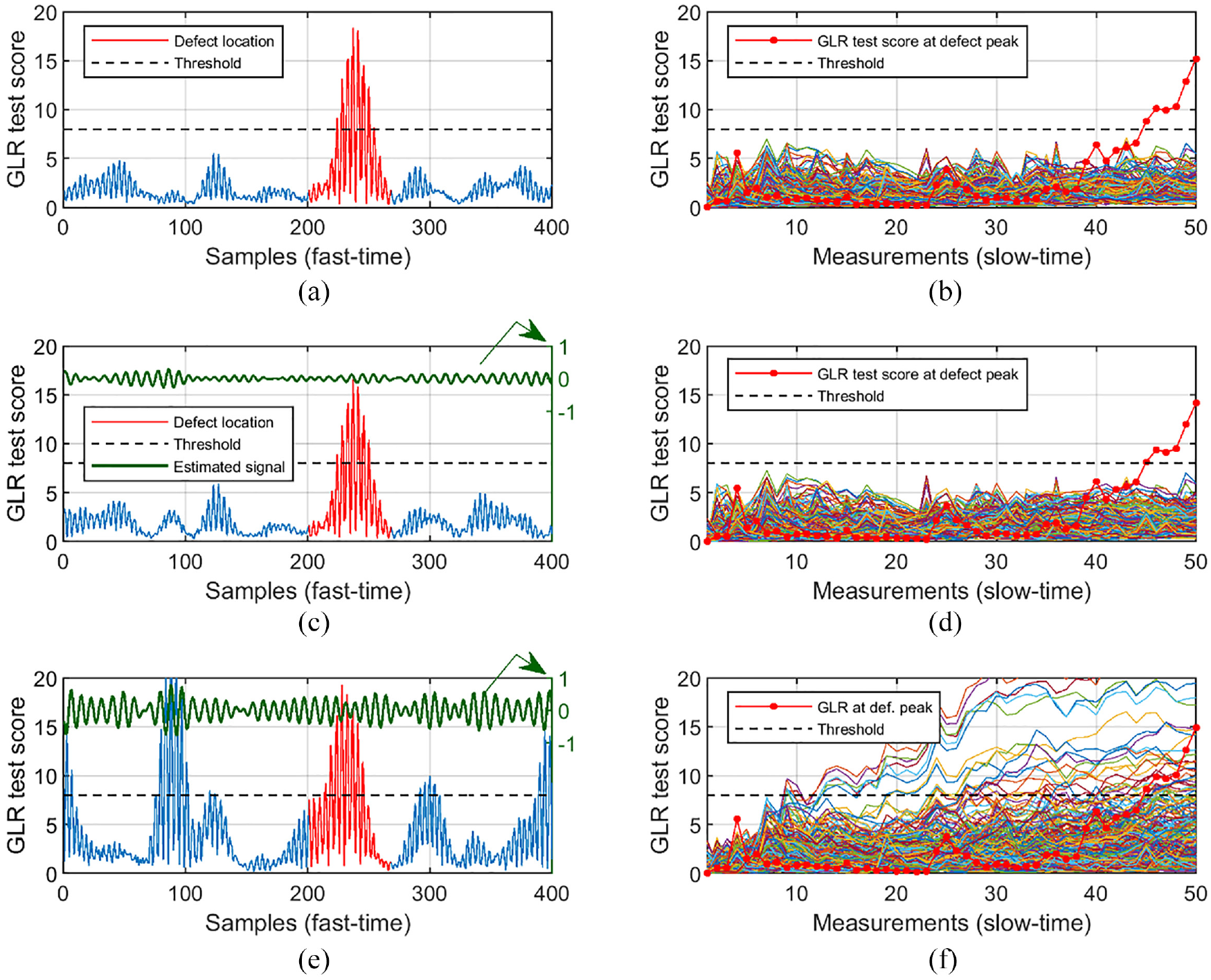
(a and b) Case of LSTC_∞: GLR test scores obtained when analyzing the case of Figure 2(b), (d) and (f) and laid out in (a) fast-time and (b) slow-time directions. A possible threshold set to 8 is also shown. Note that (b) also plots the GLR test scores obtained at each intermediate step, and only plots the scores at the defect peak (sample 233) and those away from the defect location, indicated in blue in (a). (c and d) Case of LSTC₁₀₀: plots analogous to (a and b), except that the estimated underlying signal obtained by averaging the considered 100 baselines is also given, in green (right-hand scale, showing amplitude with respect to standard deviation). (e and f) Case of LSTC₁₀: plots analogous to (c and d). Legend in (e) same as (c).

In the idealized scenario described so far, where the true underlying signal was deemed to be completely known (case of LSTC_∞), the sensitivity does not depend on the number of baseline signals available to calibrate the LSTC compensation method (or rather, it actually refers to the case of having an infinite number of baselines). In this scenario, by taking a larger number of current measurements that include a defect reflection, one would always improve the sensitivity, on average (or, at worst, it would not degrade it). Nevertheless, in realistic scenarios, N_BAS will have to be considered as an added hyperparameter when investigating the defect detection performance, since it will greatly affect it. For example, Figure 3(c) to (f) considers the same case analyzed so far (same 50 current signals), but when using N_BAS equal to 100 and 10, respectively, to calibrate the LSTC method, that is, to estimate the true underlying signal to be subtracted from each of the 50 current signals to obtain residuals, which will then be fed to the GLR method. For the two specific instances of the two sets of baseline signals being randomly generated, the estimated underlying signals are the two green plots in Figure 3(c) and (e), one for each of the two cases. The other features plotted in Figure 3(c) to (f) are obtained analogously to those in Figure 3(a) and (b). It appears that, at least in this specific considered instance, LSTC₁₀₀ produces results very similar to those of LSTC_∞, that is, without an appreciably decreased sensitivity. However, Figure 3(f) shows that if only 10 baselines are used, there will be many false calls if the presence of the considered defect is to be called. This shows that the number of baseline signals must be sufficient that the average incoherent noise level across the baselines is reduced to a substantially lower level than the level of defect reflection that must reliably be detected, as confirmed by the results of the analyses discussed in the following sections. Importantly, in this scenario of a small number of baselines, taking more current measurements and so feeding longer sequences of residuals to the GLR algorithm is not always beneficial, and can actually be detrimental, since the GLR test scores at undamaged locations where the estimate of the underlying signal is significantly different to its true value will grow with increasing number of samples and so lead to more false calls. Nevertheless, as will be shown in the following, even when low N_BAS values are available, it is still possible to detect larger defects with an acceptably low PFA rate, by carefully selecting a sufficiently high threshold value and by setting a limit on the length of sequences of residuals to be fed to the GLR method. This can be done with a one-in one-out approach, such that once the set limit length is reached, the earliest measurement is discarded and the latest is added to the set of current signals to be analyzed via GLR.

Monte Carlo analysis and generation of receiver operating characteristic curves

Monte Carlo analyses were performed to investigate the PD and PFA rates for a given length of fast-time signal. Figure 4 shows a schematic of the procedure that was used to study the defect detection performance obtained for various scenarios. First, a set of N_BAS undamaged baseline signals was created, comprising 1, 10, or 100 measurements. Then, the same number N_SIG of undamaged and defective current signals were generated, N_SIG being 1, 10, or 100. In the next step, all current measurements were compensated using LSTC_∞, ${\mathrm{LSTC}}_{N_{\mathrm{BAS}}}$ , or ${\mathrm{OBS}}_{N_{\mathrm{BAS}}}$ (note that, as explained in the previous section, the results of LSTC_∞ do not depend on N_BAS). Finally, the three sets of residuals (each set comprising both undamaged and defective subsets) were fed to the GLR method, that is, processed via equation (5) with μ₀ = 0 and σ = 1. Note that for the cases of N_SIG set to 1, where the GLR method applied to only one signal sample would not be beneficial, the defect call was made from the value of the residual directly, as is done with standard baseline subtraction methods. ⁵ This series of steps was repeated one million times, so that at each iteration, entirely new sets of baseline and current signals were analyzed and the variability of the process was correctly captured.

Figure 4.

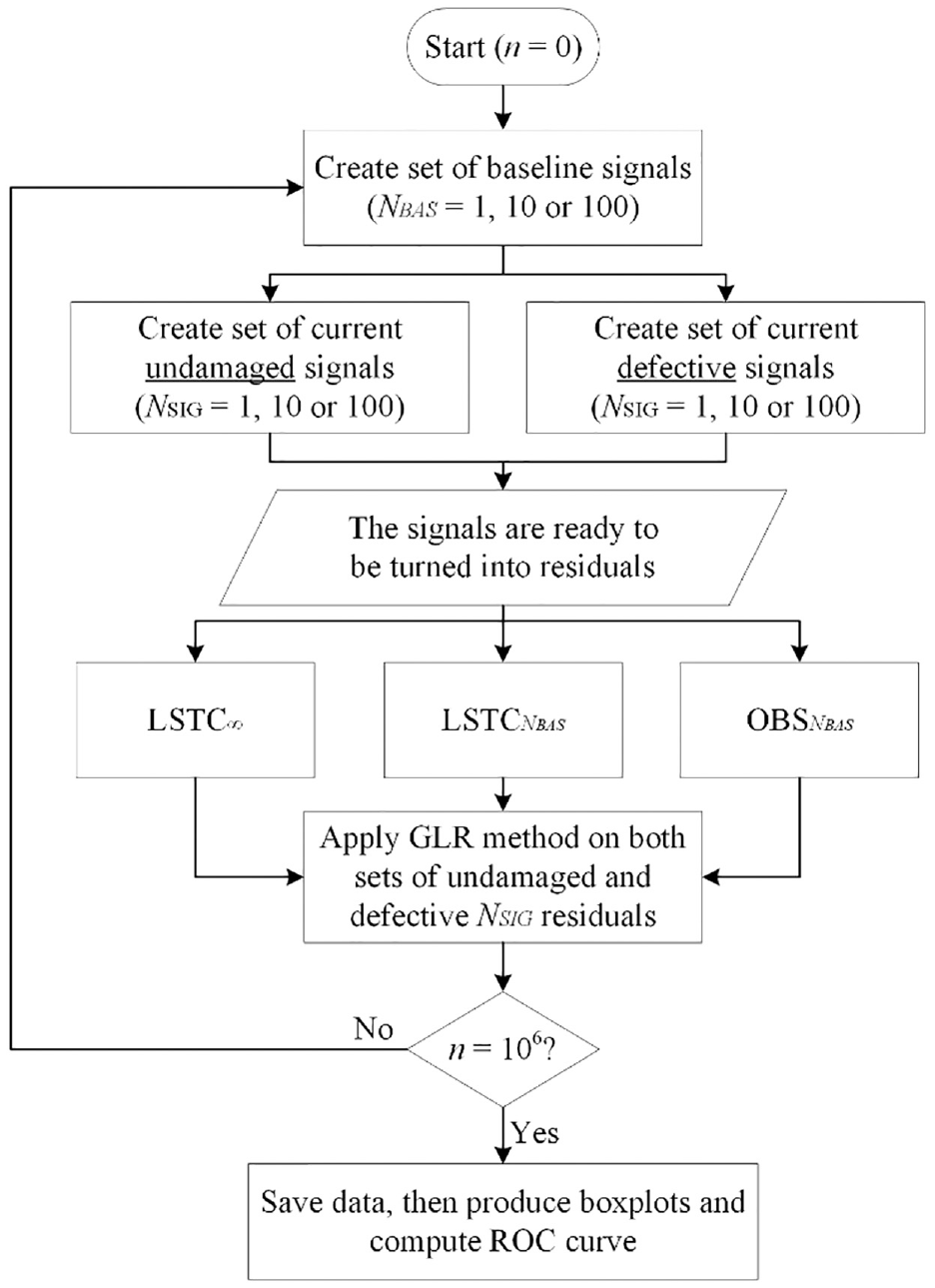
Flowchart describing the entire process followed to perform the Monte Carlo analyses whose results are given in section “Results.”

As seen in the last step of Figure 4, once the complete set of data from one million iterations was obtained, each subset belonging to one of the three examined cases of LSTC_∞, ${\mathrm{LSTC}}_{N_{\mathrm{BAS}}}$ , and ${\mathrm{OBS}}_{N_{\mathrm{BAS}}}$ was processed to compute two types of result: (1) boxplots showing either the distributions of the maximum absolute values of residuals, when N_SIG = 1, or those of the maximum GLR test scores, when N_SIG > 1, and (2) a receiver operating characteristic (ROC) curve, following the procedure illustrated in Figure 5.

Figure 5.

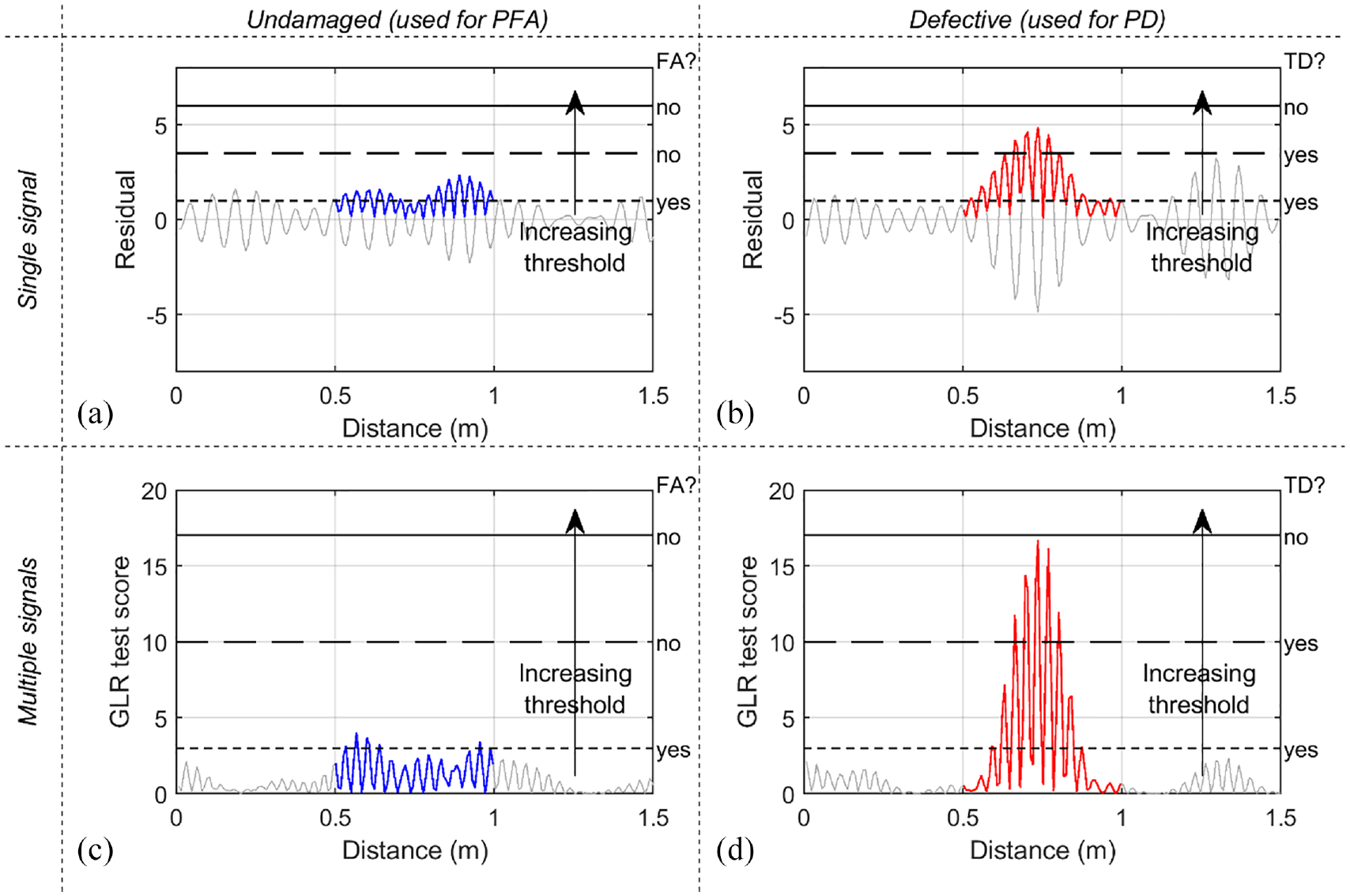
Procedure used to extract PFA (a and c) and PD (b and d) rates in order to compute the ROC curves of section “Results.” (a and b) refer to the case of N_SIG = 1, where the GLR method is not executed and the threshold is compared to the absolute values of residuals. (c and d) refer to the other cases (N_SIG > 1), where the threshold is compared to the GLR test scores. The 0.5 m long portions of signals of interest are only those highlighted in blue (a and c) or red (b and d). As the threshold is gradually increased from zero, a false alarm (FA) or a true detection (TD) is noted if the maximum amplitude within the module exceeds it. For example, in each plot, the three decisions corresponding to three different threshold levels are illustrated.

The experimental study presented in section “Experimental validation” considers a pipe monitored using the T(0,1) guided wave where each temporal position in the time trace of a measurement is related to a specific structural position via the wave speed. At the 23.5-kHz center frequency used, given the 3.2 km/s wave speed, the spatial extent of the eight-cycle excitation toneburst is about 0.5 m so this is the length of the reflection from a simple defect. Therefore, when determining whether a defect is detectable at a given threshold “call” level, it is necessary to search over a 0.5 m length centered on the middle of the defect reflection. In order to determine the PFA at each threshold level, it is necessary to search signals with no defect added; the PFA level is proportional to the length of signal searched since there is equal probability of an excursion above the threshold anywhere in the signal. Therefore, the Monte Carlo simulations for PFA also used a 0.5 m length of signal, and the results are expressed per half meter of pipe, although they can readily be extended to longer monitoring lengths as explained in the next section.

Figure 5(a) and (b) shows the procedure used for the case of N_SIG = 1, and hence plot residual signals rather than GLR test scores. The 0.5 m long portions of signals used for the generation of an ROC curve are those highlighted in blue (Figure 5(a), undamaged signal used for the PFA) or red (Figure 5(b), defective signal used for the PD), although signals over distances longer than 0.5 m were generated, as discussed below. The threshold is gradually increased from zero, and a FA, or a true detection (TD), is noted if the absolute value of residual at any sample within the relevant portion exceeds it. The numbers of FAs and TDs at each threshold are divided by the total number of available undamaged and defective signals (both equal to one million), hence giving estimates of the PFA and PD rates, which allow an ROC curve to be constructed. Figure 5(c) and (d) refers to cases of N_SIG > 1, and hence shows GLR test scores as obtained by processing the available signals via equation (5) with μ₀ = 0 and σ = 1. The procedure used to compute PFA and PD rates is analogous to that of Figure 5(a) and (b), although here the threshold is compared to the GLR test scores rather than residual amplitudes.

Unlike LSTC, OBS gives slightly different results depending on the total signal length considered, since it performs a “global” compensation as described in section “Simulation of undamaged signals and application of LSTC or OBS to generate residuals.” Therefore, the signals generated for the Monte Carlo analyses described in this section were 8 m long, rather than the 0.5 m used in the ROC generation as this length is more representative of real pipe inspection scenarios; Figure 5 only shows 1.5 m of the 8 m for clarity. For the same reason, it is more challenging to generalize the results produced by OBS, so unlike the case of LSTC, the PD and PFA rates found in this study cannot readily be extended to cases of shorter or longer signals. It should be noted that the exact position of the 0.5 m long portions analyzed within the total signal length does not influence the results of either OBS or LSTC.

Results

Figure 6 summarizes the distributions of the maximum absolute values of residual registered for cases of N_SIG = 1, where the GLR method was not used. The two plots refer to N_BAS of 1 and 10 (Figure (a) and (b)). Each plot comprises five frames, each of which includes three boxplots that show the results obtained by processing the signals via LSTC_∞, ${\mathrm{LSTC}}_{N_{\mathrm{BAS}}}$ , and ${\mathrm{OBS}}_{N_{\mathrm{BAS}}}$ . A single boxplot consists of a box, a horizontal line, and two whiskers, which indicate, respectively, the interquartile range, the median, and the 99.98% two-sided interval of the values. The leftmost frame refers to the undamaged measurements obtained via the procedure illustrated in Figure 1, while the other four frames refer to signals containing a defect reflection introduced as shown in Figure 2, where each frame corresponds to a different defect peak amplitude with respect to the incoherent noise affecting the simulated measurements. Specifically, the defect sizes considered in this figure are 3, 6, 9, and 12 times the standard deviation of the incoherent noise level. Clearly, when the whole of a boxplot referring to a given defective case, and obtained via a specific compensation process among LSTC_∞, ${\mathrm{LSTC}}_{N_{\mathrm{BAS}}}$ , and ${\mathrm{OBS}}_{N_{\mathrm{BAS}}}$ , is above the corresponding undamaged boxplot representing the same compensation method (i.e. when the bottom whisker of the defective case exceeds the top whisker of the undamaged case), then the relevant defect size can be detected with at least 99.99% PD and at most 0.01% PFA. Note, however, that precise estimates of very low levels of PFA would require more than 10⁶ realizations.

Figure 6.

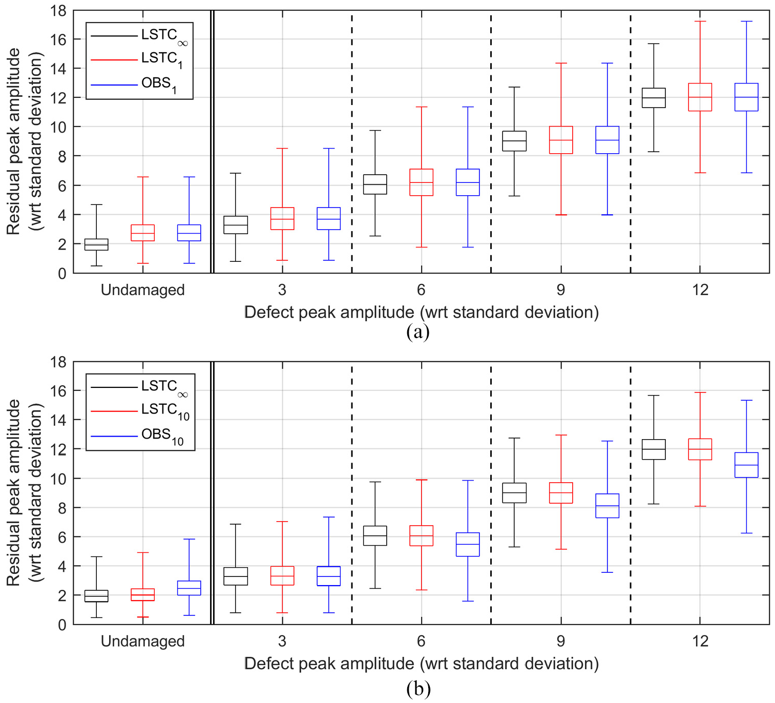
Boxplots summarizing the maximum values of residuals obtained for cases of N_SIG = 1. The two plots refer to cases of N_BAS equal to (a) 1 and (b) 10. In each plot, the leftmost frame refers to the pristine residual signals, and the other four frames refer to the defective signals, at increasing defect sizes. In each frame, the three boxplots correspond to the compensation technique used to produce residuals, this being either LSTC_∞, ${\mathrm{LSTC}}_{N_{\mathrm{BAS}}}$ , or ${\mathrm{OBS}}_{N_{\mathrm{BAS}}}$ . The box, the horizontal line, and the whiskers indicate, respectively, the interquartile range, the median, and the 99.98% two-sided interval of the values.

When N_BAS = 1, both LSTC₁ and OBS₁ perform simple baseline subtraction using the only available baseline signal; hence, red and blue boxplots in Figure 6(a) are identical. Note that when baseline and current measurements are acquired at identical temperatures (as in the scenario considered in this section), the residual at each signal sample is a random variable obtained by subtracting two independent normal variables distributed as N(μ_und, σ²) and N(μ_und + μ_def, σ²), respectively, where μ_und is the true signal value at the given sample in undamaged conditions, μ_def is the true amplitude of defect reflection at the same sample if a defect is present in the current measurement (μ_def = 0 otherwise), and σ is the standard deviation of the incoherent noise affecting the measurements, as before. Therefore, according to the rules of sum and linear transformations of normal distributions, the residual obtained by subtraction is also a normal variable distributed as

$$N({\mu }_{\mathrm{und}}+{\mu }_{\mathrm{def}}-{\mu }_{\mathrm{und}},{\sigma }^2+{\sigma }^2)=N({\mu }_{\mathrm{def}},2·{\sigma }^2)$$

(8)

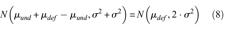
Since in this study it was assumed that σ = 1, the residual at each sample is a normal variable with mean equal to zero (for undamaged cases), or the size of defect reflection at the given sample (for defective cases), and standard deviation of $\sqrt{2}$ . Therefore, in order to maintain very low PFA rates, the minimum defect size that can reliably be detected in this scenario has to be substantially larger than unity. Hence, among the four defect sizes analyzed in Figure 6(a), only the boxplot corresponding to the largest of the defects is entirely above that of the undamaged signals (when using LSTC₁ or, identically, OBS₁). On the other hand, for an exactly known true undamaged signal (scenario of LSTC_∞), the residuals are distributed as N(μ_def, σ²), that is, the standard deviation decreases by a factor of $\sqrt{2}$ . As a result, the black boxplots referring to LSTC_∞ in Figure 6(a) show that defects of size 9 can now be reliably detected (as would be expected since $12/\sqrt{2}\cong 8.5$ ).

When multiple baselines are available, the calibration of LSTC becomes more accurate, and the red boxplots of Figure 6(b), referring to LSTC₁₀, appear almost identical to the black boxplots pertaining to LSTC_∞. Only minor improvements are then obtained with LSTC₁₀₀, whose results are not shown here for brevity. A comparison of the results offered by LSTC₁₀ with those of LSTC₁ shows an overall reduction of the residuals as captured by the red boxplot in the undamaged frames, which is beneficial to keep the PFA rates low, and a reduction of the variability around almost unchanged median values for the defective cases. Here, the increased residual values representing the bottom half of each distribution guarantee higher PD rates. Therefore, with LSTC, it can safely be concluded that as N_BAS increases, the defect detection performance improves. The OBS results are more difficult to interpret; while the blue boxplots in the undamaged frames also shift to lower values as N_BAS increases (although remaining higher than those offered by LSTC), which is beneficial in terms of PFA, with OBS a similar trend also occurs in the defective cases (for the reasons given at the end of section “Simulation of undamaged signals and application of LSTC or OBS to generate residuals”), hence penalizing the PD rates. Therefore, depending on which of the two effects prevails, in OBS, an increase of N_BAS will not always correspond to a better defect detection performance.

Figure 7 shows the ROC curves based on the signals containing defects of size 6, as N_BAS increases from Figure 7(a) 1 to Figure 7(b) 10. Effectively, this better investigates the defective case already illustrated in the central frame of Figure 6(a) and (b). The curves obtained using LSTC_∞, ${\mathrm{LSTC}}_{N_{\mathrm{BAS}}}$ , and ${\mathrm{OBS}}_{N_{\mathrm{BAS}}}$ are plotted in black, red, and blue, respectively. Each plot is on semi-logarithmic scale, since in most monitoring applications low FA rates would be required, and the light gray dashed line is the random guess performance (which in a linear plot would be an ROC curve following the 45° diagonal line, where the PD and PFA are equal). As already described, when N_BAS = 1 (Figure 7(a)), LSTC₁ and OBS₁ give identical results (here, a dashed line is used for OBS to allow the two curves to be seen), and their performance is much poorer than that of LSTC_∞. However, as already expected from the analysis of Figure 6(b), when 10 baselines are available, the results of LSTC₁₀ are already very similar to those that would be given by N_BAS = ∞, as seen in Figure 7(b). By contrast, the blue ROC curves of Figure 7(a) and (b) reveal that in this case, the performance of OBS remains essentially unchanged.

Figure 7.

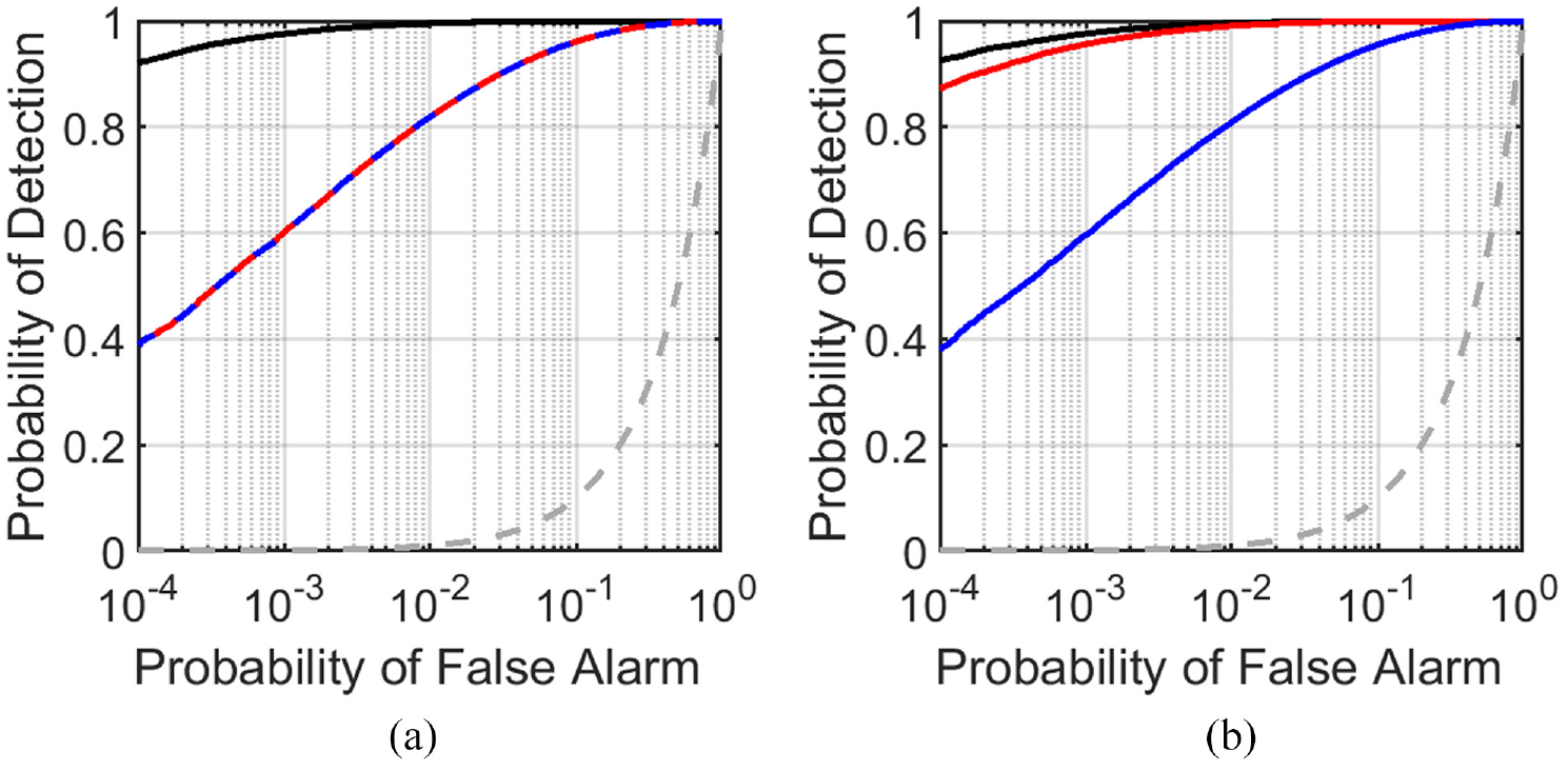
ROC curves for N_SIG = 1 and defects of size 6. N_BAS equal to (a) 1 and (b) 10. The curves obtained using LSTC_∞, ${\mathrm{LSTC}}_{N_{\mathrm{BAS}}}$ , and ${\mathrm{OBS}}_{N_{\mathrm{BAS}}}$ are plotted in black, red, and blue colors, respectively. The light gray dashed line is the random guess performance (which in a linear plot would be an ROC curve following the 45° diagonal line, where the PD and PFA are equal). Note that each plot is on the semi-logarithmic scale.

On a practical note, even the performance offered by LSTC_∞ of Figure 7 might still be unsatisfactory in many monitoring applications if a defect of this size must be reliably detected. For example, if the “call threshold” corresponding to PFA = 0.01% and PD ≈ 92% (i.e. the y-axis intercept of the black curves) is used to monitor a 10 m long pipe, every time a new current measurement is acquired there will be 0.2% probability of a false call (20 times the PFA rate for 0.5 m shown in the figure), and 92% probability of calling a defect of size 6 if that is present (note that, unlike PFA, the PD rates given in this study do not depend on the length of the monitored signal, so do not need to be rescaled).

The performance can be improved if multiple current measurements are acquired and analyzed via the GLR method. This is first investigated in Figure 8, which refers to cases of N_SIG = 10 and considers defects sized at 1, 2, 3, and 4. The plots refer to N_BAS of 1, 10, and 100 (Figure 8(a) to (c)). Each plot is analogous to that of Figure 6, although here smaller defects are investigated and the boxplots refer to GLR test scores. When only a single baseline signal is available, as in Figure 8(a), the results obtained via LSTC₁ and OBS₁ are identical. The variability in the computation of each individual residual signal, which was discussed previously, prevents any significant improvement from using the GLR method, and the defect detection performance that can be achieved for defects of size 4 (or smaller) is unsatisfactory. If N_BAS = 10, as in Figure 8(b), the performance offered by GLR when fed with residuals produced by LSTC₁₀ substantially improves, thus enabling a virtually perfect detection of defects of size 4. Further improvements are gained when 100 baselines are available, as seen in Figure 8(c) where the performance obtained via LSTC₁₀₀ is close to that of LSTC_∞, and defects of size 3 are reliably detected. The black boxplots in Figure 8 indicate that this is roughly the minimum defect size that can be detected with virtually zero FAs when feeding the GLR with sequences of residuals of length 10 (i.e. using the considered case of N_SIG = 10). Finally, as was already observed in Figure 6, the GLR test scores achieved when using OBS to produce residuals decrease in both undamaged and damaged cases as N_BAS increases.

Figure 8.

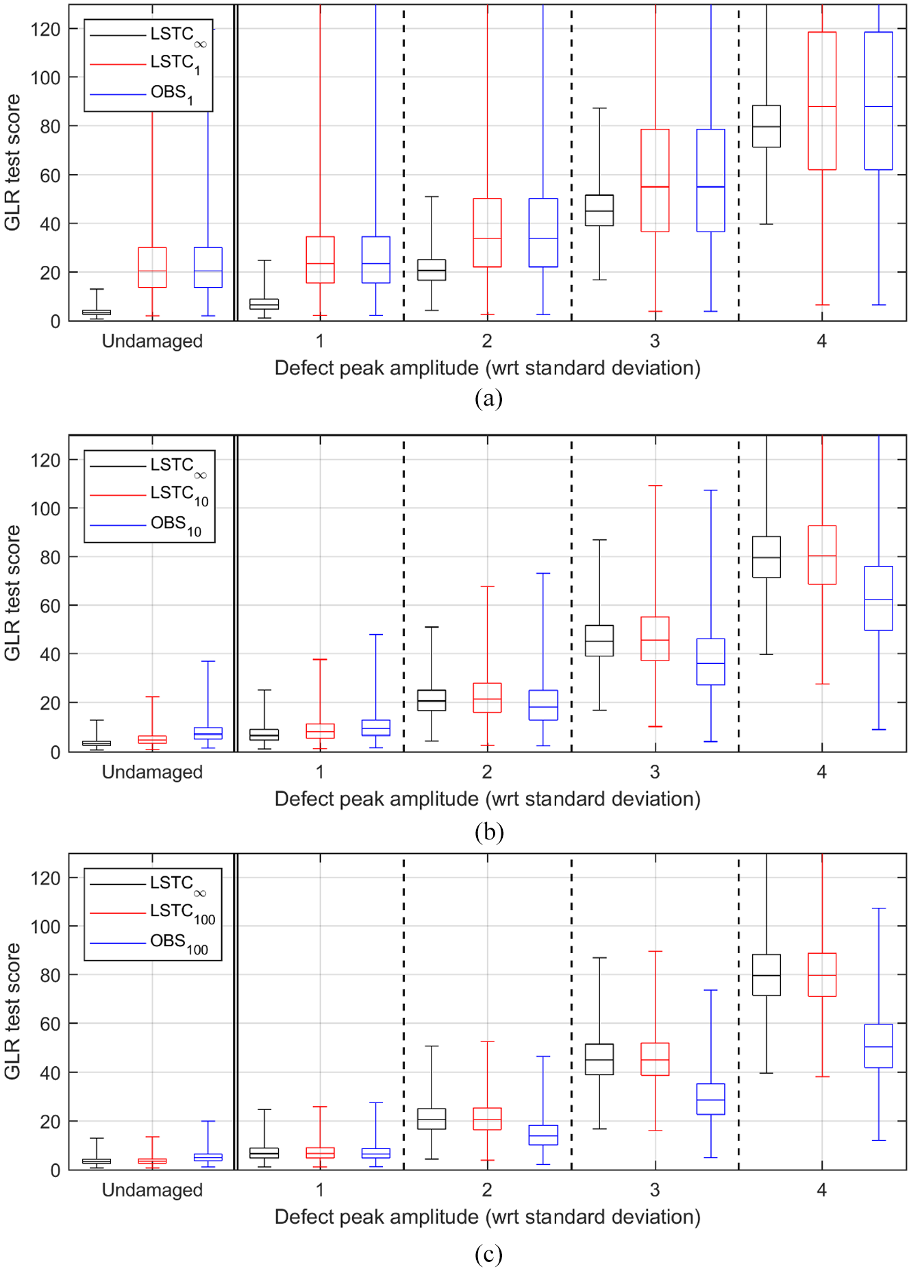
Boxplots summarizing the GLR test scores obtained for N_SIG = 10. The three plots refer to cases of N_BAS equal to (a) 1, (b) 10, and (c) 100. In each plot, the leftmost frame refers to the pristine residual signals, and the other four frames refer to the defective signals, at increasing defect sizes. In each frame, the three boxplots correspond to the compensation technique used to produce residuals, this being either LSTC_∞, ${\mathrm{LSTC}}_{N_{\mathrm{BAS}}}$ , or ${\mathrm{OBS}}_{N_{\mathrm{BAS}}}$ . The box, the horizontal line, and the whiskers indicate, respectively, the interquartile range, the median, and the 99.98% two-sided interval of the values.

Figure 9 shows the ROC curves computed for defects of size 2 (a to c) and 3 (d to f) when N_SIG = 10, and as N_BAS increases. As expected, when N_BAS = 1 (Figure 9(a) and (d)), LSTC₁ and OBS₁ are effectively the same and provide identical performance. Substantial improvements are seen via LSTC₁₀ and even more with LSTC₁₀₀ when targeting either defect, and, as discussed above, Figure 9(f) confirms that the application of GLR on residuals produced by LSTC₁₀₀ to target defects of size 3 gives virtually perfect detection with, at most, 0.01% PFA (none of the one million Monte Carlo iterations performed for this defect size gave a lower score than any of those obtained in the undamaged scenario; hence, the PFA is likely to be lower than 0.01%). Finally, Figure 9 shows that in this case, unlike that of Figure 7, increasing N_BAS improved the performance of OBS, although it remained less good than LSTC.

Figure 9.

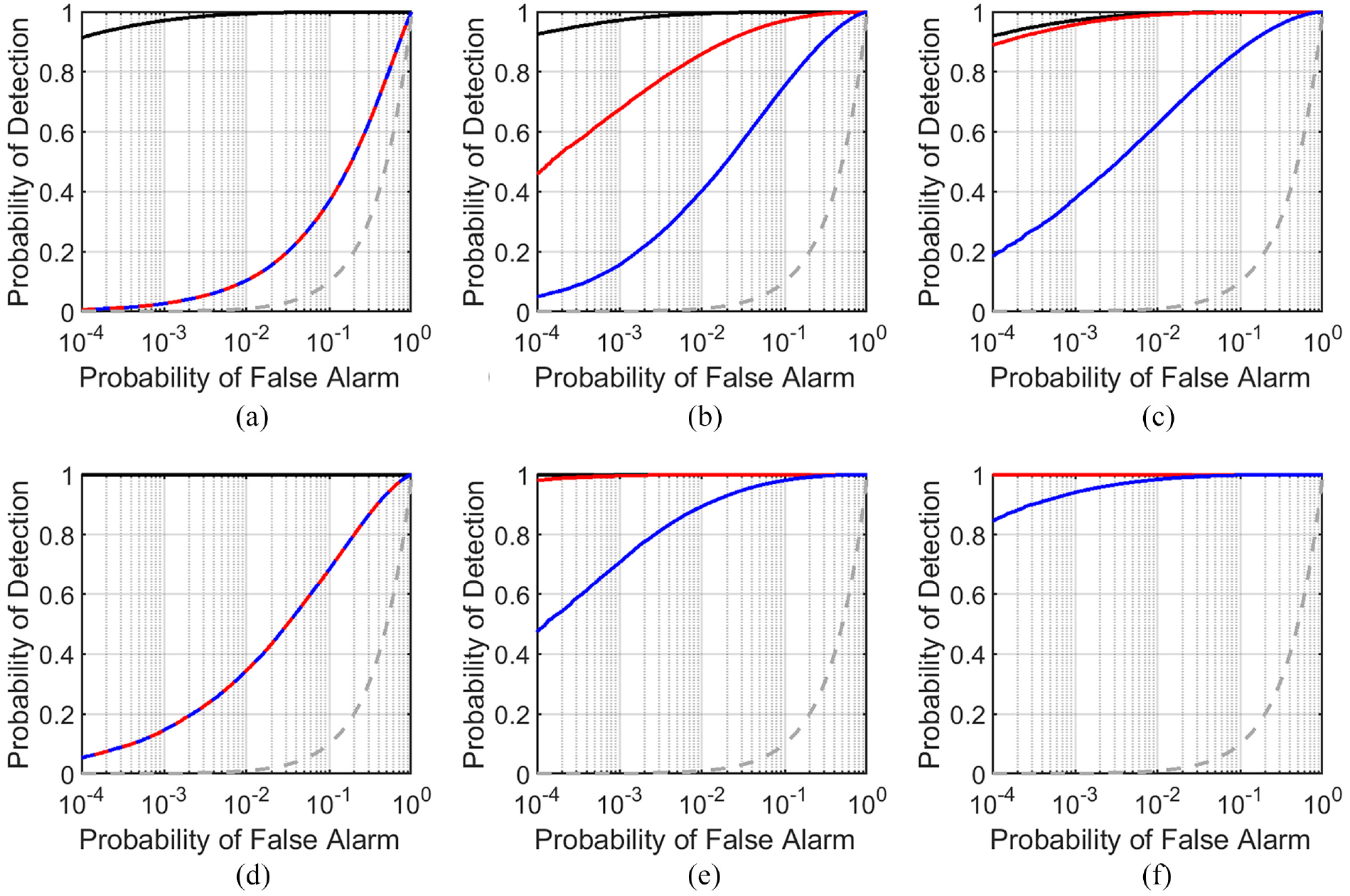
ROC curves for N_SIG = 10 and defects of size (a to c) 2 and (d to f) 3. N_BAS equal to (a and d) 1, (b and e) 10, and (c and f) 100. The curves obtained using LSTC_∞, ${\mathrm{LSTC}}_{N_{\mathrm{BAS}}}$ , and ${\mathrm{OBS}}_{N_{\mathrm{BAS}}}$ are plotted in black, red, and blue colors, respectively. The light gray dashed line is the random guess performance (which in a linear plot would be an ROC curve following the 45° diagonal line, where the PD and PFA are equal). Note that each plot is on the semi-logarithmic scale.

Finally, Figure 10 analyzes the case of N_SIG = 100 and N_BAS = 100, with defects ranging from 0.5 to 2 in steps of 0.5. The trend of improving detection performance with number of current signals and number of baselines continues, and using LSTC, a defect reflection 1.5 times the incoherent noise level is reliably detectable with virtually zero false calls. Figure 10 also shows that there are now appreciable differences between LSTC₁₀₀ and LSTC_∞, indicating that more baselines would now give further improvement. For example, LSTC_∞ here allows virtually perfect defection of defects of size 1 with virtually zero FAs. This suggests that as the goal shifts to detect increasingly smaller defects (which would always be enabled by increasing N_SIG if residuals were produced by LSTC_∞), an increasing number of baselines, N_BAS, is needed to asymptotically approach the best-case scenario represented by LSTC_∞. In other words, an increasingly accurate calibration of LSTC is needed to effectively drive the sensitivity to detect sub-standard deviation changes. This puts a practical limit to the sensitivity that can be achieved in most monitoring applications, where often N_SIG can be conveniently increased (simply by taking more current measurements on the test structure at the unknown health state), but the number of baselines acquired earlier on (when the structure was defect-free or in a constant damage condition) is limited. These improvements from analyzing more data are, of course, dependent on the key assumptions of section “Change detection algorithm for SHM” remaining valid, notably that the residuals can be assumed to remain normally distributed and there is no sensor drift with time. These assumptions are increasingly questionable as the target defect reflection decreases in amplitude.

Figure 10.

Boxplots summarizing the GLR test scores obtained for N_SIG = 100 and N_BAS = 100. The leftmost frame refers to the pristine residual signals, and the other four frames refer to the defective signals, at increasing defect sizes. In each frame, the three boxplots correspond to the compensation technique used to produce residuals, this being either LSTC_∞, ${\mathrm{LSTC}}_{N_{\mathrm{BAS}}}$ , or ${\mathrm{OBS}}_{N_{\mathrm{BAS}}}$ . The box, the horizontal line, and the whiskers indicate, respectively, the interquartile range, the median, and the 99.98% two-sided interval of the values.

Multiple tests at varying temperature

Creation of the test data set

The goal of the study presented in this section is to investigate the extent to which the application of LSTC temperature compensation enables results obtained over a significant operating temperature range to approach the detection performance demonstrated in the previous section with measurements obtained at constant temperature; as before, the performance offered by OBS in this scenario is also investigated. In this scenario, the LSTC method requires a set of baseline measurements sparsely acquired across the predicted operating temperature range to construct calibration curves that give the expected signal amplitude at each signal sample (corresponding to a particular location on the structure) in the absence of damage and as a function of temperature. It has been shown that the signal at each sample varies smoothly with temperature, so fitting the available baseline measurements with a polynomial of appropriate order provides excellent results. ⁶ As a general rule, the larger the range of operating temperature variations, the higher the order of polynomial needed to capture the oscillatory signal variations with temperature; this is discussed further in section “Investigation on the calibration curves produced by LSTC.” Measurements acquired outside the temperature range of the baseline set are discarded, since extrapolation of the calibration curves outside the baseline temperature range can lead to large errors. ³⁸

“Ground truth” signals that undergo realistic variations due to temperature were needed to set up Monte Carlo analyses similar to those described in the previous section. In pipe monitoring, rather complicated interactions between unwanted circumferential and flexural modes generate coherent noise that varies with temperature at any given signal sample, corresponding to a particular location on the pipe. ⁵ This coherent noise is usually insignificant at the detection thresholds used in one-off non-destructive testing (NDT) inspection, but becomes significant in monitoring where the aim is to detect smaller defects reliably. The experimental data set discussed in more detail in section “Experimental validation” was used to provide an example of the variation in signal amplitude with temperature at each location along a pipe. The data set contains 250 measurements performed at temperatures ranging from 30°C to 90°C using the first order torsional guided wave mode on a straight portion of pipe.

When signals are acquired at different temperatures, the time of arrival of the reflection from damage at a given structural location varies slightly from one measurement to another, depending on the relevant wave velocity at the specific test temperature. It is important to ensure that measurements taken at different temperatures are correctly “registered” so that a given location on the time trace corresponds to the same spatial location in all the measurements; this can be achieved by applying a standard method of temperature compensation such as the BSS method ⁸ that compensates the measurements for the changing wave speed with temperature. This was therefore applied to the 250 measurements before the variation in amplitude with temperature at each location was extracted using a best-fit polynomial. It should be stressed that this analysis was simply used to generate a representative data set showing the typical variation of signal amplitude with temperature away from the locations of reflectors in the pipe, that is, the variation of the coherent noise with temperature; similar levels of variation have been observed on more complex pipe systems in the lab and in field tests, so it is believed that the data set is representative of what will be found in practice. There is no suggestion that this is the absolute “true” relationship between coherent noise in the experiments and temperature since in reality this is subject to statistical measurement uncertainty, but it can be used as the “ground truth” in Monte Carlo investigations of defect detection performance as required here.

Figure 11 illustrates the resulting “ground truth” signal model. As in the previous section, signal amplitudes are given with respect to the standard deviation of the incoherent noise that was measured from the experimental data set (see section “Investigation on the calibration curves produced by LSTC” for details). Figure 11(a) shows the variation of coherent noise with temperature corresponding to seven locations on the pipe (out of 248 sampling points along the 2 m long portion of monitored pipe). Figure 11(a) also shows three examples of the “true” underlying signal that can be directly sampled from the curves at any desired temperature within the available range. The seven curves showing the variation with temperature are shown in a two-dimensional plot in Figure 11(b) to show more clearly the extent of coherent noise fluctuations as the temperature varies. The three time traces of Figure 11(a) are plotted in Figure 11(c), using different colors. The “ground truth” signal at any desired temperature in the 60°C range can be obtained by selecting the appropriate signal level at each location from curves of the type shown in Figure 11(b). In the Monte Carlo analyses described in this section, a temperature in the 60°C range was selected (a resolution of 0.1°C was used in this study), the “ground truth” time trace was generated, and an incoherent noise time trace produced in the manner described in section “Simulation of undamaged signals and application of LSTC or OBS to generate residuals” was superposed on it. To generate a defective case, a defect reflection of the desired size with respect to the standard deviation of the incoherent noise was then added at the desired signal location using the methodology of Figure 2.

Figure 11.

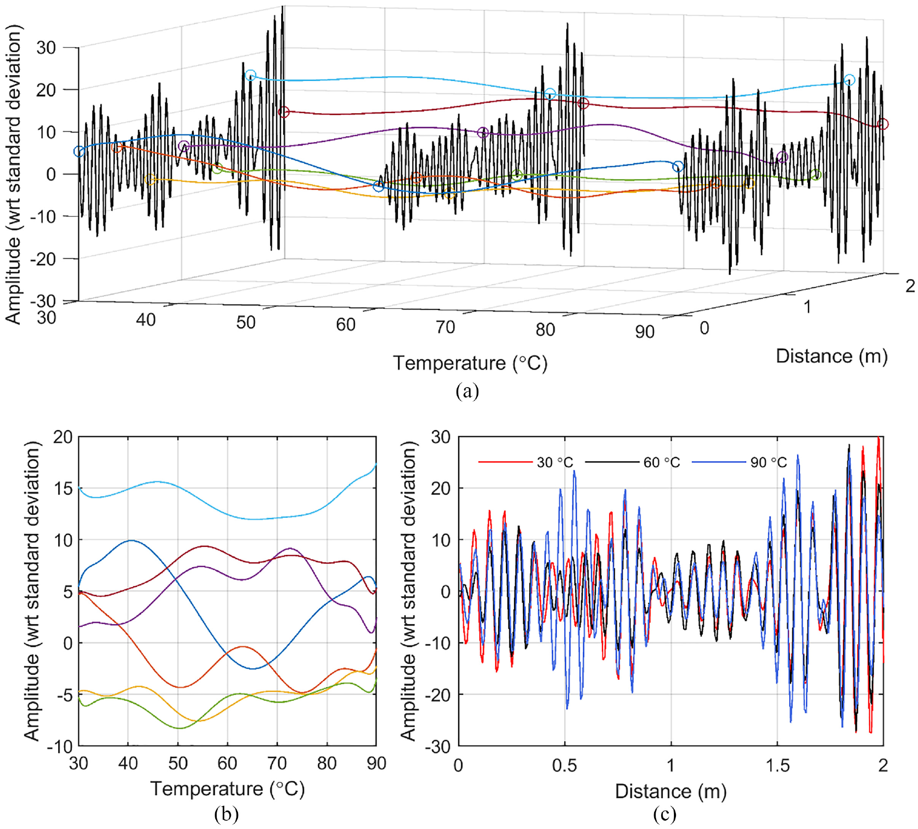
“Ground truth” signal model used to perform the Monte Carlo analyses for measurements taken at different temperatures. (a) Example signals at three different temperatures (black) and example polynomial curves corresponding to seven locations on the pipe (out of 248 used to sample the 2 m long portion of monitored pipe) that fit the variation in signal level as a function of temperature. (b) The seven curves shown in a 2D plot to aid clarity. (c) The black curves of (a) shown superposed in different colors to highlight the differences between them.

The procedure used to study the defect detection performance was again that of Figure 4, although here only the case of N_BAS = 100 was considered, since N_BAS = 10 (or 1) would be insufficient to produce very accurate results over the 60°C wide temperature range considered here. At each iteration, N_BAS baseline signals and N_SIG undamaged and damaged measurements were generated by picking random temperatures within the available temperature range (although the baseline set was forced to always include at least one measurement at both 30°C and 90°C, so the operating temperature range was always 60°C). In each iteration of the Monte Carlo analysis, the LSTC method was set to fit the N_BAS baseline measurements with polynomial curves of order 12, as shown in Figure 12. These calibration curves were then used to predict the coherent noise level at each location along the pipe at the given temperature; this was then subtracted from the “current” signal to produce the residual signal. ⁶ LSTC_∞ assumed perfect knowledge of the true underlying signal at any temperature, and so was again independent of the particular N_BAS acquired at each iteration. OBS, as in the previous section, used equation (7) to select the best baseline measurement for compensation of any specific current measurement. As for the previous case of testing at fixed temperature (Figure 5), the maximum absolute value of residuals (if N_SIG = 1) or the maximum GLR test score (if N_SIG > 1) was searched over a 0.5 m long signal portion, whose exact position within the 2 m long signal does not influence the results of LSTC, but in this scenario can influence those of OBS, as discussed in the next section. Therefore, at each iteration and for either undamaged or defective cases, the location of the 0.5 m long portion was selected at random.

Figure 12.

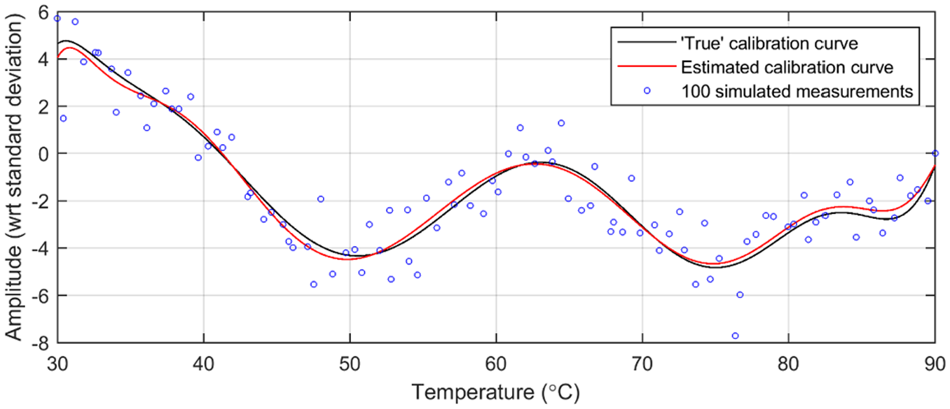
“True” LSTC calibration curve for the signal sample located at 0.4 m, compared to the curve estimated when using the 100 simulated measurements shown with blue circles.

Figure 12 shows an example of a calibration curve produced by LSTC₁₀₀ at the signal sample located at 0.4 m (location of the orange curve of Figure 11(a) and (b)). Note that in actual monitoring, the “true” calibration curve is unknown and can only be exactly estimated if a very large number of baseline signals are collected at all temperatures (i.e. case of LSTC_∞). However, in this study, the true curves are perfectly known since they correspond to the “ground truth” model that was constructed as described above. The 100 measurements acquired at random temperatures within the temperature range were used by LSTC₁₀₀ to produce the red calibration curve, which shows good agreement with the “true” black curve. The average difference between the estimated and “true” curves across the entire temperature range was computed over multiple iterations at all signal locations, and at all locations, it was found to have a standard deviation of ∼0.1, that is, the value expected from the Bienaymé formula for n = 100 (see section “Simulation of undamaged signals and application of LSTC or OBS to generate residuals”). This indicates that, on average, the calibration curves produced by LSTC when testing at varying temperature are offset from the true underlying signals by a similar amount as for the case of testing at fixed temperature. This suggests that the defect detection performance is likely to be similar to that obtained at constant temperature; this will be tested in the next section.

Results

Figure 13 shows boxplots representing the GLR test scores for the case of N_BAS = 100 and N_SIG = 100. The plot is analogous to that of Figure 10, to which it can be directly compared. The performances when using LSTC₁₀₀ and LSTC_∞ are essentially unchanged from those seen in the fixed temperature case; hence, the application of GLR to the residuals produced by LSTC₁₀₀ still allows defects giving reflections 1.5 times the incoherent noise level to be detected. By contrast, all boxplots pertaining to OBS₁₀₀ are shifted to lower values. This occurs since, in this scenario, when a defect is present, OBS has the chance to select a baseline measurement taken at a temperature further away than the closest available with respect to that of the current measurement, if that produces overall lower residuals according to equation (7), hence partially suppressing the defect reflection. The likelihood of this happening can also depend on the relative position (phase mismatch) between the defect reflection and the coherent noise present across the signal length, which was the reason for randomizing the defect location over multiple iterations. Similarly, for undamaged measurements, this process can attenuate some large peaks that can be produced at random by the incoherent noise. In this particular case, these concomitant effects give a slightly better performance than that obtained in the fixed temperature scenario, although OBS remains significantly inferior to LSTC.

Figure 13.

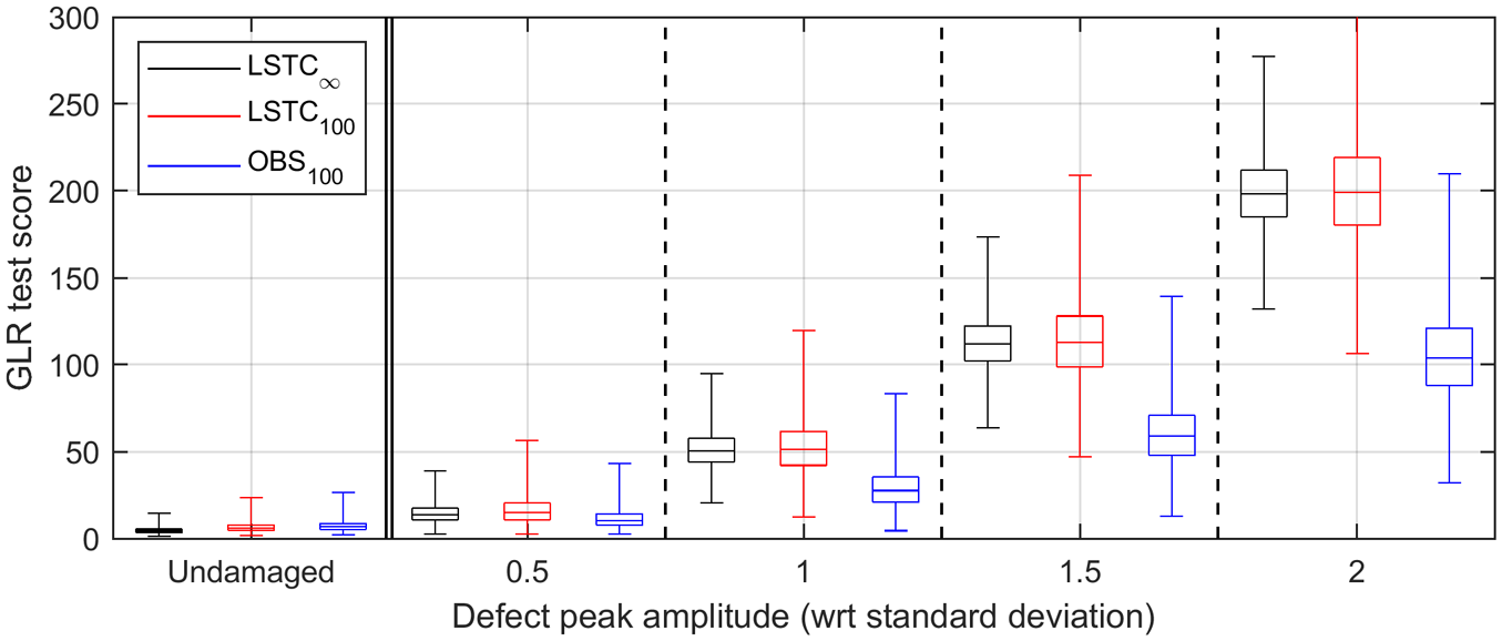
Boxplots summarizing the GLR test scores obtained for the case of N_BAS = 100 and N_SIG = 100. In each plot, the leftmost frame refers to the pristine residual signals, and the other four frames refer to the defective signals, at increasing defect sizes. In each frame, the three boxplots correspond to the compensation technique used to produce residuals, this being either LSTC_∞, ${\mathrm{LSTC}}_{N_{\mathrm{BAS}}}$ , or ${\mathrm{OBS}}_{N_{\mathrm{BAS}}}$ . The box, the horizontal line, and the whiskers indicate, respectively, the interquartile range, the median, and the 99.98% two-sided interval of the values.

The comparison of the results obtained for cases of N_SIG = 1 and N_SIG = 10 at varying temperature against the corresponding ones at fixed temperature leads to analogous conclusions; hence, those results are not shown, for brevity. Therefore, the main conclusion of this study is that using the LSTC temperature compensation method based on polynomial fitting of the variation of coherent noise with temperature seen in baseline measurements at each location on the structure gives defect detection performance that is virtually identical to that obtained in tests at constant temperature. However, when measurements are acquired at varying temperature, a minimum number of baselines is needed to correctly “guide” the polynomial interpolation within the whole operating temperature range, this number being strictly dependent on the rate of coherent noise variation with temperature that is specific to the particular monitoring application, since that will also depend on the rate of change of interference with position between unwanted propagating modes. Further studies conducted on the available data set showed that, in pipe monitoring, no appreciable loss of performance for a given number of baselines compared to the constant temperature scenario would be obtained if sufficient baselines are available to sample the operating temperature range roughly every 2°C–3°C.

Experimental validation

The GLR method described in this article was applied to a data set of ultrasonic guided wave signals acquired by a Guided Ultrasonics Ltd. gPIMS sensor ring ²⁵ set to use the T(0,1) wave mode. The sensor ring was attached to a 5 m long, 8-in schedule 40 pipe which had a heating element inside the pipe, allowing its temperature to be cycled; the outside of the pipe was insulated so the temperature dropped slowly after being heated to the desired maximum temperature and the heating element switched off. The ring was installed 3.5 m from the right-hand end of the pipe as shown schematically in Figure 14(a). The excitation was an eight-cycle toneburst centered at 23.5 kHz, and the sampling rate was set at 200 kHz. The measurements used to perform the analysis reported in this article are those in the “forward” direction indicated in Figure 14(a). The pipe was subjected to heating and cooling cycles between 30°C and 90°C, and a total of 250 measurements were acquired during the cooling phases, as seen in Figure 14(b) that shows the pipe temperature measured by a sensor installed near the sensor ring.

Figure 14.

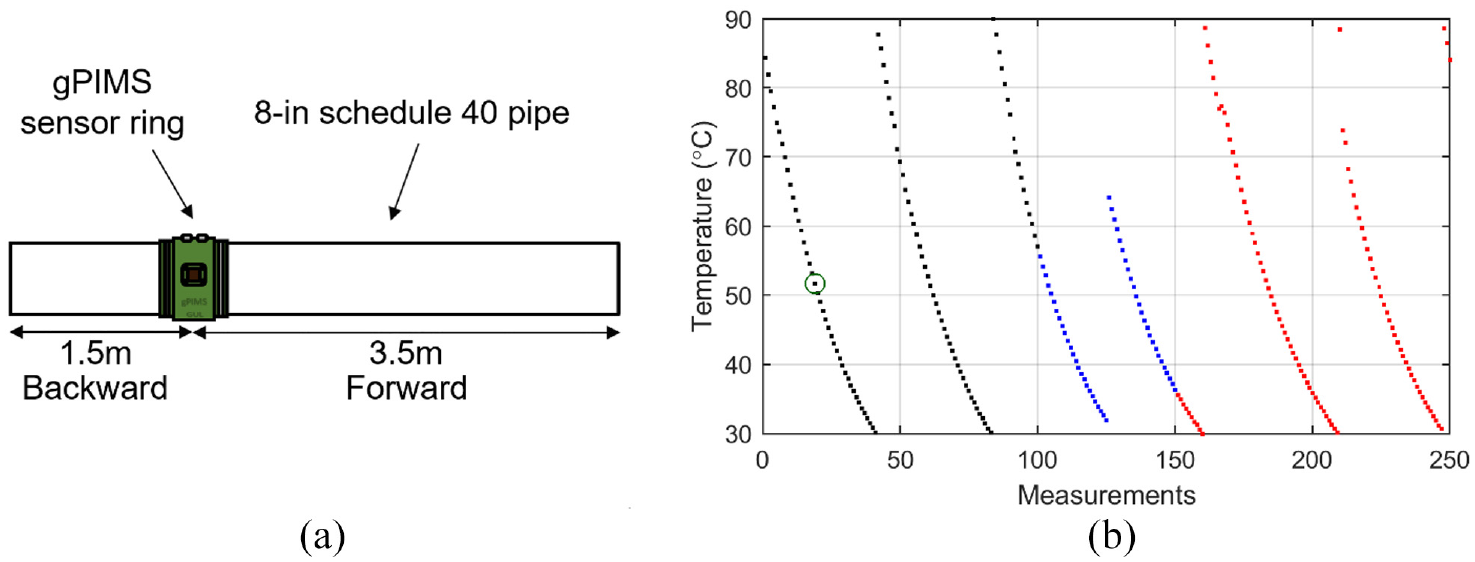
(a) Geometry of the 8-in schedule 40 test pipe; the distances are measured from the middle of the sensor. The measurements used to perform the analysis reported in this article are those in the “forward” direction. (b) Temperature of the pipe during the tests. The green circle indicates measurement #19, which is shown in Figure 15 and which was used as baseline for the BSS temperature compensation method. The first 100 measurements (in black) and the last 100 (in red) were used as sets of “baseline” and “current” measurements, respectively, in the study discussed in section “Example of application of GLR to the residuals produced by LSTC.”

Figure 15 shows the measurement that was used as baseline for the BSS temperature compensation method, ⁸ which was needed to compensate for the varying T(0,1) wave speed at the different measurement temperatures, and which was performed prior to the application of the LSTC compensation method ⁶ for the reasons given in section “Creation of the test data set.” In Figure 15, the time-domain ultrasonic signal is converted to distance using a T(0,1) velocity of 3240 m/s, which was estimated from the arrival time of the reflection from the end of the pipe and the known pipe length. The measurements corresponding to the 2 m of pipe closest to the end were used in the analysis; this ensured that they were well clear of any near-field effects that may have been present and that were not part of this study.

Figure 15.

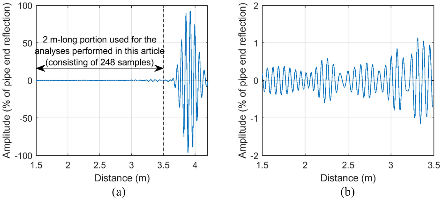
(a) Measurement #19 acquired at 51.7°C and used as baseline for the BSS temperature compensation method. ⁸ In (b), the vertical scale is reduced to better display the 2 m long portion of pipe used to construct the “ground truth” signal model of Figure 11(c) and to perform the analyses described in sections “Investigation on the calibration curves produced by LSTC” and “Example of application of GLR to the residuals produced by LSTC.”

Investigation on the calibration curves produced by LSTC

An investigation was conducted using the whole set of 250 experimental signals to determine the best order of polynomial capable of capturing the true underlying coherent noise variations occurring as the temperature varied over the 60°C wide range. Two parameters were measured as the polynomial order was sequentially increased, these being the overall standard deviation of residuals obtained by subtracting the actual measurements from the curves fitted with each order of polynomial, and the likelihood of the set of residuals obtained at each sample location on the pipe being normally distributed. The likelihood that a sequence of readings is produced by an underlying normally distributed process can be estimated using a “frequentist test” such as the Shapiro–Wilk (SW),^39–41 which is generally considered to be the test giving the highest probability of correctly rejecting the null hypothesis of normal distribution for a given significance. ⁴² Therefore, the SW test was applied to the sequence of 250 residuals obtained at each signal sample, for a total of 248 samples corresponding to the sample locations along the 2 m long portion of pipe shown in Figure 15, with the test significance set at 1%. From the definition of significance level, there is a 1% probability that the test will return a false positive result (i.e. an incorrect rejection of the null hypothesis of normal distribution when that is actually true), that is, ∼2.5 false positives on average over the 248 samples analyzed at each step.

Figure 16(a) shows the standard deviation of residuals measured across all samples as the order of polynomial fitting was increased. The curve decreases sharply as the order is increased up to roughly the 10th degree, then decays more slowly, indicating that the oscillation of coherent noise with temperature across the 60°C wide range is essentially captured by a polynomial of order 10. The number of samples for which the SW test refuted the null hypothesis of normality at each polynomial order is given in Figure 16(b); the scatter on the curve is due to the limited number of samples available. After an early significant decrease (103 and 39 positives for first and second degree of polynomial, respectively, not shown at the vertical scale of the plot), the trend reaches a minimum around the 12th order, before rising again at higher orders as the data become overfitted. Note that the three positives that are obtained when using order 12 are in line with the expected 1% false positive rate. These findings are visually substantiated when comparing the three fitting curves shown in Figure 16(c) and (d), which refer to the same signal sample investigated in Figure 12. Figure 16(c) shows the optimum order 12 fit, while Figure 16(d) shows the order 3 and 22 fits. It is clear that an order 3 polynomial severely underfits the underlying variations of the data across the temperature range, while an order 22 polynomial overfits it. The order 12 polynomial provides a good fit, as already indicated by the parameters analyzed in Figure 16(a) and (b). Visual inspection of the curves obtained at the other locations on the pipe confirmed this finding. Therefore, polynomials of order 12 were used to perform the analyses described in this article.

Figure 16.

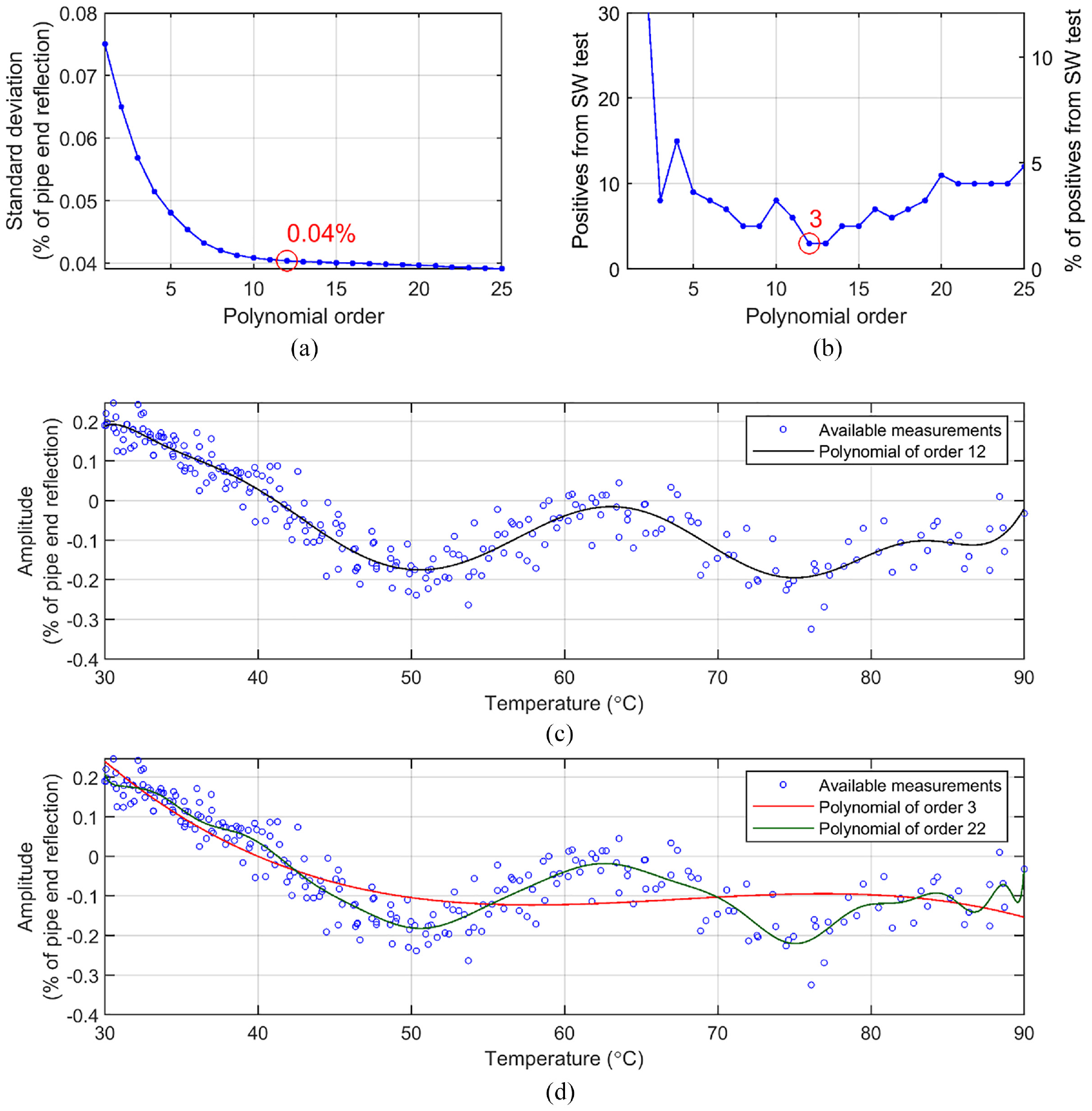
Investigation using the whole set of 250 experimental signals to determine the best order of polynomial capable of capturing the true underlying coherent noise variations with temperature across the 60°C wide test range. (a) Overall standard deviation of residuals across all samples. (b) Number of samples for which the Shapiro–Wilk (SW) test refuted the null hypothesis of normality. Values highlighted in red in (a and b) are those for the chosen order of 12. Polynomial curves obtained by fitting the measurements at the sample located at 1.9 m with a polynomial of (c) order 12 and (d) order 3 and 22. Note that this is the same sample investigated in Figure 12.

The complex variation of the coherent noise level with temperature at each location on the pipe is the result of interference between multiple unwanted modes that are excited at much lower levels than the desired torsional mode and which have different velocities and different temperature coefficients of velocity.

Example of application of GLR to the residuals produced by LSTC

This section shows an example of the application of the GLR method to the experimental data set described above. As shown in Figure 14(b), in this study, the first 100 measurements were selected as baseline signals for the LSTC temperature compensation method, which was set to fit the baseline observations using polynomials of order 12. The calibration curves were then used by LSTC to extract residual signals from the 100 “current” measurements shown in red in Figure 14(b). Since the pipe was left undamaged during the tests, introduction of damage was simulated by superposing onto the actual experimental signals the reflection expected from a defect producing uniform frequency response ³⁶ at the desired amplitude, that is, following the procedure validated in Heinlein et al. ³⁷ and already used in section “Simulation of damage and application of GLR method.” A representative scenario among those analyzed in Figure 13 is considered, namely, the detection of a defect giving a reflection 1.5 times the standard deviation of incoherent noise affecting the measurements. As seen in Figure 16(a), the noise level was estimated at 0.04% with respect to the reflection from the end of the pipe; hence, a defect reflection amplitude of 0.06% was considered. Note that in long-range pipe monitoring using the T(0,1) wave mode, the ratio between the reflection from a defect and the amplitude of the propagating T(0,1) signal (i.e. virtually identical to that reflected from the end of the pipe) is typically on the order of the fraction of the pipe cross section removed by the defect. ²⁰ The results of the analyses performed on purely simulated measurements that are discussed in section “Multiple tests at varying temperature” can be used to set a sensible threshold to inspect GLR test scores obtained from actual experimental measurements such as those considered in this section. For example, Figure 13 suggests that when GLR is applied to 100 residual signals obtained via LSTC compensation based on 100 baseline measurements, a good choice for the threshold on GLR test scores would be to set it at 30, which would give virtually zero false calls as long as the key assumptions of section “Change detection algorithm for SHM” remain valid (i.e. in the absence of sensor drift with time).

Figure 17 summarizes the results obtained from the application of the GLR method to 100 experimental residual signals computed via LSTC applied either (a to d) on the original undamaged current measurements or (e to h) on the measurements including the simulated 0.06% defect. Figure 17(c) plots the LSTC residuals computed from the undamaged measurements of Figure 17(a), the first five of which are also plotted in three dimensions (3D) in Figure 17(b) to better appreciate the random nature of their content (note the similarity with the simulated random signals of Figure 1(a)). As expected, the GLR test scores shown in Figure 17(d) are on the order of magnitude described by the red boxplot in the leftmost frame of Figure 13 and no false calls are made. The introduction of the simulated defect reflection of Figure 17(e) to the undamaged measurements of Figure 17(a) does not produce any noticeable change when simply looking at the “defective” A-scans of Figure 17(f), but once coherent noise is removed via the application of LSTC, careful observation of the residuals in Figure 17(g) reveals some degree of coherence at the defect location, as expected. After GLR is applied, the defect detection becomes obvious since the GLR test scores at the defect location of Figure 17(h) significantly exceed the set threshold. The registered peak value is about 100, which is in line with the red boxplot corresponding to a defect 1.5 times the standard deviation of noise shown in Figure 13.

Figure 17.

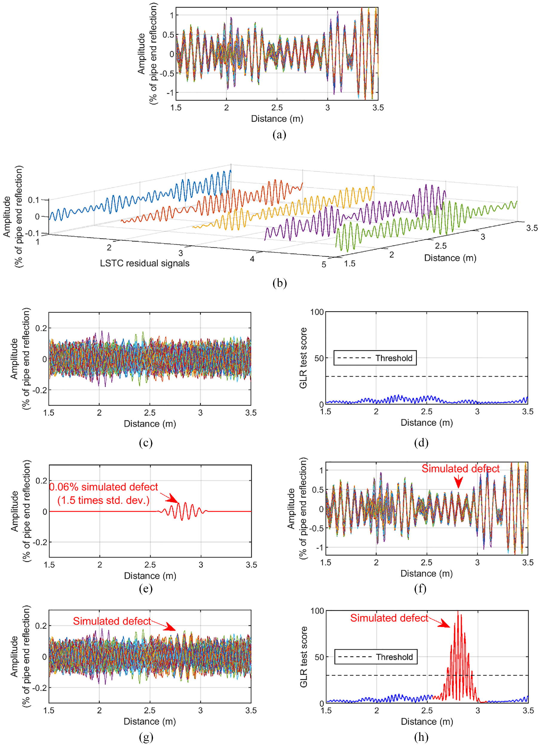
(a to d) Undamaged case: (a) 100 undamaged “current” measurements (shown in red in Figure 14(b)); (c) residual signals computed by LSTC (the first five of which are also 3D plotted in three dimensions in (b)), which were fed to the GLR method obtaining the GLR test scores in (d). (e to h) Damaged case: the simulated defect reflection in (e) was added by superposition to the undamaged 100 measurements of (a) obtaining the “defective” signals shown in (f); (g) residuals computed by LSTC that were fed to the GLR method producing the GLR test scores in (h).

Conclusion

This article presented a framework based on the GLR change detection method applied to residual signals produced by LSTC or OBS temperature compensation techniques to enhance the defect detection performance achievable in guided wave–based SHM. In principle, due to the nature of the GLR method, increasingly smaller defects can be detected by delaying the time of call in order to keep the false call level to a minimum, with the delay expressed in terms of number of measurements taken on the test structure after damage actually occurred, although this is limited by the uncertainties in removing temperature effects.

The defect detection performance was analyzed on simulated signals that were generated using as reference an experimental data set collected by a pipe monitoring system designed to monitor tens of meters of pipe from one location using the torsional, T(0,1), guided wave mode. First, the case of testing at fixed temperature was analyzed in great detail by considering different scenarios regarding the available number of baseline signals, the number of current signals analyzed by the GLR method, and the defect reflection size with respect to the standard deviation of incoherent noise affecting the measurements, that being essentially due to instrumentation noise. Then, the analysis was extended to the more practical case of testing across a large operating temperature range (between 30°C and 90°C in the analyzed scenario), and it was shown that essentially the same results can be obtained as those for the fixed temperature scenario, provided that enough baseline signals spread across the temperature range are available. In all analyzed cases, the performance offered by GLR when applied to the residuals produced by LSTC was better than that given by GLR on the residuals obtained via the widely used OBS temperature compensation method. It was shown that, as expected, the performance depends on the number of available baseline signals, which determines the precision of temperature compensation, and on the number of signals analyzed by the GLR method, which is related to the likelihood of making a true defect detection; for example, using a sufficient number of baseline and current signals, reliable detection of small defects giving reflection 1.5 times the standard deviation of incoherent noise is possible with virtually zero false calls—this reflection size roughly corresponding to damage producing 0.1% cross section loss of pipe or less.

The results were partially validated using the experimental signals by showing that the residuals produced by the LSTC method are normally distributed, which is a key assumption of the framework, and that the GLR test scores obtained on the undamaged structure are on the order of those predicted by the numerical study. Although the analyzed experimental data set did not contain any actual defect, it should be stressed that the proposed method is sensitive to departures from the residuals obtained on the undamaged structure, as would be produced by LSTC when damage occurs; ⁶ this sensitivity was tested by superposing a simulated defect reflection of amplitude 1.5 times the standard deviation of the measured incoherent noise (which would be produced by damage on the order of 0.1% pipe cross section loss). Again, the GLR test scores obtained from such hybrid experimental and simulated measurements confirmed the predictions of the numerical study.

The proposed detection framework is very attractive since it can be set to operate automatically after estimating the measurement noise from the available set of baseline signals and after setting an appropriate threshold. The methodology of the study described in this article can be used to choose the desired threshold depending on the PD and PFA that one wants to achieve with respect to some desired minimum size of defect and with respect to the maximum acceptable delay for the detection of such minimum defect size. Importantly, the delay is measured as numbers of measurements rather than strictly elapsed time; SHM systems such as that considered in section “Experimental validation” can be set to acquire measurements every few hours, although if they are battery-powered the chosen testing frequency must also consider the acceptable power consumption over time.

Importantly, the detection performance discussed in this study is dependent on the key assumptions of section “Change detection algorithm for SHM” remaining valid, notably that there is no sensor drift with time. This is increasingly questionable as the target defect reflection decreases in amplitude, since small changes occurring over time in the sensor behavior would be increasingly comparable to the former. Future studies will be aimed at identifying methods to assess the occurrence of sensor drift effects in the signals and to quantify the expected drop in performance when such effects occur, as well as developing corrective measures to counteract these effects. Finally, although the study was mainly focused on pipe monitoring systems using the T(0,1) wave mode, the measured performance expressed in terms of damage size with respect to the standard deviation of measurement noise will also essentially apply to monitoring systems using other guided wave techniques or standard bulk waves.