
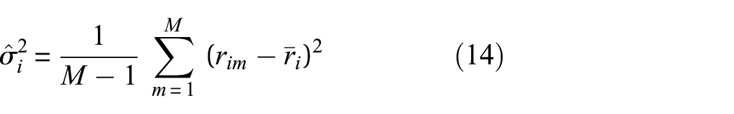
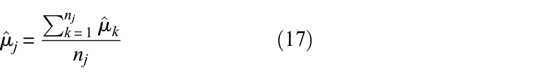
Abstract
In this article, a hierarchical approach is proposed for the design and assessment of a guided wave-based structural health monitoring system for the detection and localisation of barely visible impact damage in composite airframe structures. The hierarchical approach provides a systemic and practical way to establish guided wave-based structural health monitoring systems for different structures in the presence of uncertainties and to quantify system performance. The proposed approach is carried out in four steps: (1) determine optimal sensor placement for the target structure and its plausible impact scenarios, (2) set detection threshold for global damage index based on the noise level present in the required environmental and operations conditions, (3) detect damage in critical locations and quantify detection performance by calculating the probability of detection, probability of false alarm and detection accuracy and (4) locate the detected damage while also quantifying the accuracy of location estimation and the probability of correctly indicating if the damage is in an area critical to the integrity of the structure. The proposed approach is demonstrated in aircraft carbon fibre-reinforced polymer structures from coupon level (simple flat panels) to sub-component level (large flat panel with multiple carbon fibre-reinforced polymer stringers and aluminium frames) for the detection and localisation of barely visible impact damage.
Keywords
Introduction
The transformation of aircraft maintenance from the current schedule-based strategy to a faster, smarter and automated way of maintenance is inevitable in the age of Industry 4.0. Great effort has been directed in both academia and industry over the past few decades towards the research and development of structural health monitoring (SHM) as a new way of maintenance that aims for the efficient and continuous assessment of structural integrity.1,2 However, there are still many challenges left in developing an SHM system for commercial aircraft. These challenges include not only in the development of sensor network and the interpretation of sensor data but also in the establishment of validation methods and certification criteria for the commercial use of SHM systems. 3
Ultrasonic guided wave has been recognised to be practical in interrogating large plate-like structures due to its capability to propagate over long distances with minimal energy loss.4,5 Guided wave-based structural health monitoring (GWSHM) systems provide information on structural integrity based on measurements obtained from transducers, such as piezoelectric and fibre optic sensors. These sensor measurements are influenced by changes in environmental and operational conditions (EOC), as well as the presence of electrical noise. This causes a significant level of uncertainty in the sensor measurements which cannot be ignored and requires the application of statistical analysis techniques to take into account their effects. To add further complication, the EOC can have different effects on guided waves depending on the material as well as the type of damage present. 6 To achieve highly accurate damage identification using GWSHM systems under the required service conditions for an aircraft, the uncertainties due to EOC mentioned earlier, as well as the uncertainties in the characteristics of the damage, must be quantified for the range of materials present in the aircraft.
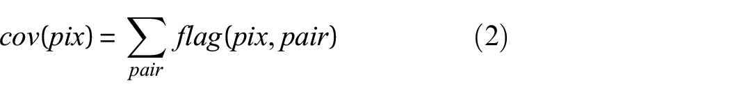
To obtain information regarding the existence of structural damage, guided wave features that are sensitive to the presence of damage can be extracted and fused to form a damage index that represents the current state of the integrity of the structure. A threshold value for the damage index can be used to distinguish a damaged state from an undamaged state. This threshold value is determined based on a certain level of statistical confidence in the sensor measurement under the presence of uncertainty caused by random and systemic noise.
The methods used for assessing the reliability of damage detection for SHM systems can be divided into two main groups: 7 (1) methods that conduct a signal response to damage size analysis and (2) methods that can conduct a hit/miss analysis. The former originates from the guidelines for conventional non-destructive inspection (NDI) techniques. 8 It applies if the system provides a continuous signal response correlated with damage size and reports the probability of detection (POD) and confidence limit related to damage size, known as POD(a) curve. Hit/miss analysis applies when the system returns binary results on whether or not a defect is present and is used in binary classification problems in many fields, such as machine learning and signal detection. Hit/miss analysis quantifies the probability of four detection outcomes: true positive, false positive, false negative and true negative. These four probabilities are closely related to the decision threshold, and this relationship is illustrated by a receiver operating characteristic (ROC) curve which plots the probability of true positive against the probability of false negative as the threshold value varies. 9
Many studies have been dedicated to the adoption of NDI approached for GWSHM systems for damage identification at damage-prone locations, such as bolted joints susceptible to the forming of cracks and bonded joints vulnerable to debonding. 10 Under the NDI approach, the POD(a) curve is derived from the independent inspection data for different defect sizes. 8 However, in the case of SHM systems, sensor measurements are repeatedly taken from the host structure. Therefore, the data are not independent and a POD(a) curve cannot be calculated. Schubert Kabban et al. 11 modified the POD(a) approach to handle repeated measurement data, which enabled the application of the POD(a) approach for SHM systems. Another limitation of the POD(a) approach is that the defect is solely represented by its size. Many SHM techniques, especially guided wave-based techniques are also sensitive to the shape of the defect as well as its position relative to the sensors. Gianneo et al. 12 investigated the influence of multiple crack parameters in aluminium on POD curves. It was shown that defect parameters, including crack size, guided wave incident angle and reception angle, have different levels of influence on the POD(a) curves and should be considered separately. Furthermore, the biggest challenge in establishing a POD(a) curve is arguably the tremendous amount of data required, including the defects of different types, sizes, orientations, and at different locations. Moriot et al. 13 proposed a model-assisted approach assessing guided wave-based detection and localisation of simulated damage. Damage detection was evaluated using a POD(a) approach. Although the experimental results from magnetic discs under consistent environmental conditions and finite element (FE)-simulated damage on aluminium plate agreed well, the simplified damage characteristics are unlikely to be representative of the actual damage. Yue et al. 14 proposed an empirical model to describe the damage detectability of guided waves in a pitch–catch sensor configuration. The model considered guided wave damping and wave-damage interaction, which provided a qualitative spacial distribution of probability of detecting damage in various locations.
An important advantage of GWSHM systems over conventional NDI techniques is their capability to effectively detect and localise damage in a large structure with minimum labour or machine assistance. This is particularly beneficial in the case where damage can be distributed in the structure, such as the damage caused by impact. The assessment of a GWSHM system with a POD(a) approach assumes that the GWSHM system is equivalent to conventional NDI techniques. This ignores the advantage in automation that a GWSHM system provides. An example where the POD(a) approach might not be practical for GWSHM reliability assessment is identifying the impact damage in carbon fibre-reinforced polymer (CFRP) laminate airframe structures. Unlike metallic materials where impact typically causes a visible dent or scratch, an impact event on composite materials can cause a mixture of fibre breakage, matrix cracking and delamination but remain nearly intact on the surface. If the POD(a) approach is applied, multiple variables will have to be introduced for POD curves to comprehend the complexity of the problem caused by diverse CFRP structure design, the complicated damage scenarios and material-dependent guided-wave characteristics.
Instead of following the POD(a) approach, many studies have assessed the reliability of SHM systems using a hit/miss approach. Nichols et al. 15 and Lu and Michaels 16 used ROC curves to effectively evaluate the damage detection performance for single damage. Flynn et al. 17 evaluated the performance of their GWSHM when detecting multiple through thickness holes in a stiffened aluminium panel using a modified ROC analysis. Monaco et al. 7 considered the POD and probability of false alarm (PFA) when setting the threshold for detecting impact damage in a CFRP laminate using GWSHM.
This article is focused on detecting the largest barely visible impact damage (BVID) in different CFRP composite airframe structures, and hence, the hit/miss analysis is used for quantifying the reliability of damage detection.
Once the presence of damage is detected, its location can be estimated. The localisation of damage can be important when investigating a large area or checking for damage at critical areas that can greatly compromise structural integrity (such as the bondline between the skin and a stiffener). A number of existing damage imaging methods can be used for estimating the damage location, such as the reconstruction algorithm for probabilistic inspection of defects (RAPID), 18 delay-and-sum (DAS), 19 energy arrival, 20 Rayleigh maximum likelihood estimation (RMLE) 21 and Bayesian approaches.22,23 To assess localisation performance, Flynn et al. 21 proposed two approaches: probability of location estimation error and Gaussian estimation. Moriot et al. 13 demonstrated the localisation of simulated damage and artificial damage on an aluminium plate using DAS with probability of location estimation error. In this work, two novel approaches for localisation performance are proposed: one provides a more intuitive measure of localisation accuracy and the other represents the ability of indicating damage presence in critical locations.
So far, most of the studies in uncertainty quantification and reliability assessment of GWSHM systems for CFRP structures have been carried out for simple isotropic plates. The issues with assessing GWSHM for damage identification in large and complicated composite structures are yet to be addressed. These issues include, but are not limited to, the effects of anisotropic material properties, greater dampening, and more complicated and harder to detect damage types. An appropriate approach is required to assess the functionality of the designed GWSHM system under intended EOC.
This article proposes a novel hierarchical approach for GWSHM design and assessment for the detection and localisation of BVID in CFRP composite airframe structures. The design process of an GWSHM system considers the placement of transducers, the estimation of noise level during the monitoring condition, and the selection of damage characterisation strategy and criteria. The damage detection performance is quantified by POD and PFA as well as the overall detection accuracy, while the damage localisation performance is assessed by the accuracy of the damage localisation estimates as well as the probability of correct indication of damage in critical areas. The proposed approach is applied for identifying BVID in CFRP airframe structures at difference scales, including simple CFRP panels, CFRP panels with single CFRP stiffener and CFRP panels with multiple CFRP and aluminium stiffeners.
Hierarchical approach
This section presents an overview of the proposed hierarchical approach to GWSHM system design and performance quantification, followed by the methodology used in each level of the hierarchy. Figure 1 presents a schematic of the proposed hierarchical approach for a general plate-like structure.
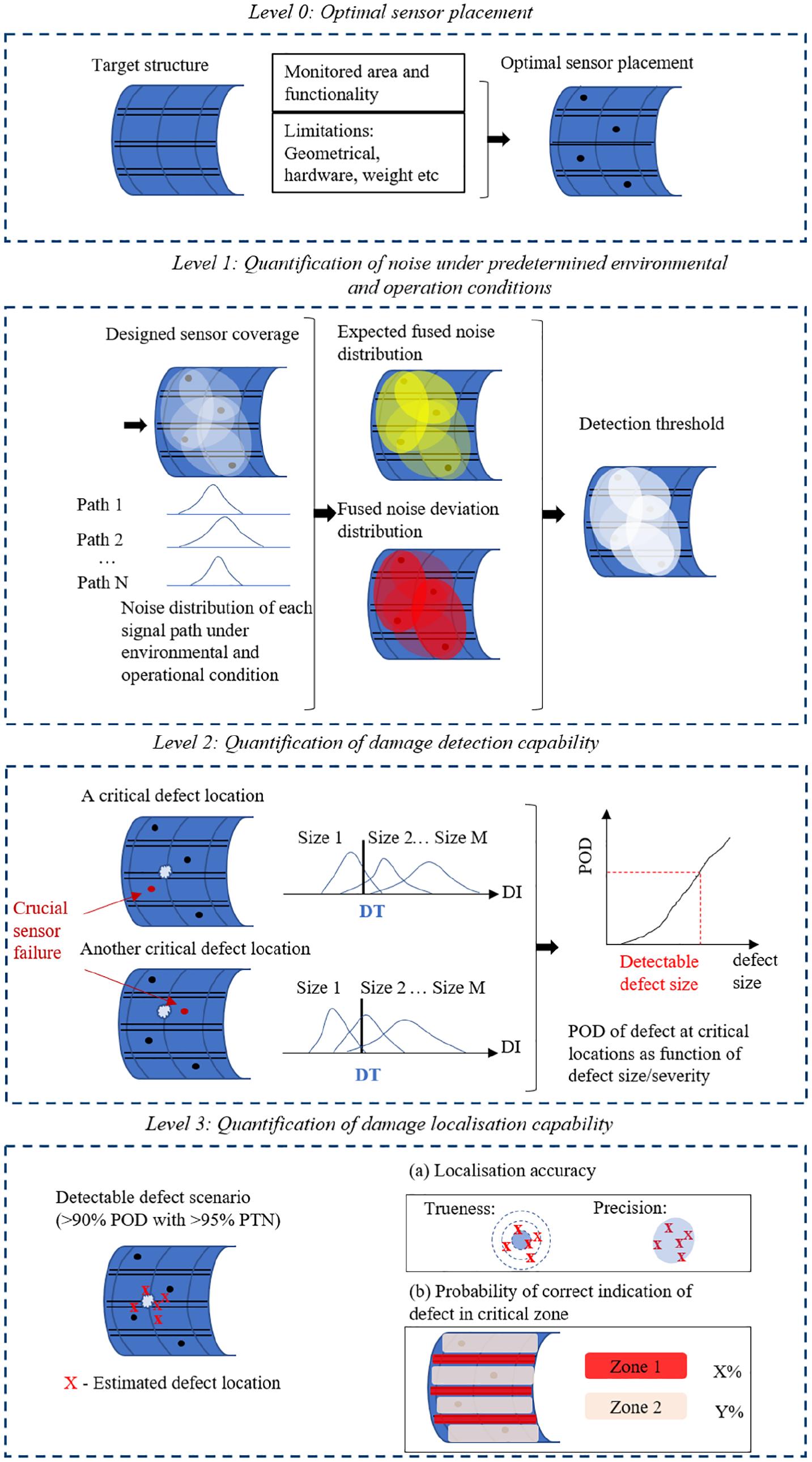
Hierarchical approach.
The considerations in each level are briefly introduced as follows.
Level 0: optimal sensor placement
For the target CFRP aircraft structure and its damage scenarios, a guided-wave SHM system can be designed to achieve effective identification of damage while minimising the overall cost. The costs associated with an industrial SHM systems can be categorised as implementation costs and in-service costs. There is a significant cost in the development of advanced technical capabilities for making the integration of sensors in modern composite structures practical and efficient so as to facilitate industrialisation and certification. The implementation cost (i.e. weight, data handling, data fusion, power consumption, etc.) can be minimised by optimising the sensor positions and by optimising the sensor installation procedure during component manufacture. The achievement of this objective should be measured by conducting a detailed cost assessment of the additional manufacturing costs associated with sensor integration including all aspects of the certification process. Sensor integration costs are an important component in the full assessment of the operative costs of the SHM-equipped aircraft.
Level 1: quantification of noise under EOC
The EOC under which the GWSHM system will be functioning is pre-defined according to the application requirement. The variability in damage-sensitive guided-wave features can then be quantified based on a number of measurements taken at the pristine state of the monitored structure at the pre-defined EOC. The damage-sensitive features from individual sensor pairs are then fused according to sensor coverage distributions by taking the average value of the damage-sensitive feature from sensor pairs that cover each position. Measures of the fused damage-sensitive feature can then be derived in the form of (1) expected fused noise distribution and (2) fused noise deviation distribution. The former describes the average value of noise and the latter is a measure of noise variability. The positions on the structure where the sensor coverage is high will have reduced variability. In other words, the more available guided-wave paths at a position, the more certain is the estimation of damage existence at that position. A global damage index (GDI) indicating the integrity state of the monitored structure is derived from the sensor network and a detection threshold can be determined based on the uncertainty of GDI in pristine state due to EOC.
Level 2: quantification of damage detection capability
With the detection threshold determined at Level 1, the damage detection can be performed in the pre-defined EOC of GWSHM. Probability of false alarm (PFA) and POD are calculated using hit/miss analysis to quantify the detection reliability. PFA indicates the chance of false calls in the varying EOC where SHM is designed to be operating, while POD is dependent on the nature and the location of the damage and is expected to be different for different damage scenarios. The most conservative approach for SHM design is to consider the worst-case scenario (the most critical damage location on the structure). The structural damage is introduced at critical locations, and the detection performance is evaluated by POD. If the probability of detecting damage at critical locations is below an acceptable value, it might be improved by increasing the number of sensors, constraining the defined GWSHM operational conditions, compensating for the damage unrelated variation in damage-sensitive guided-wave features, accepting a higher PFA by lowering the detection threshold or by accepting a greater detectable damage size (assuming POD monotonically increases with damage size/severity).
System robustness
Degradation or failure of sensors is unavoidable during long-term monitoring. According to the redundant design concept, in the event of sensor malfunction, the SHM system performance might be reduced but should remain at an acceptable level until the sensors can be repaired or replaced. It is essential to assess the influence of sensor loss on damage detection capability. The most critical sensor loss is defined as the sensor failure that leads to the most dramatic coverage reduction in the critical damage location.
Level 3: quantification of damage localisation capability
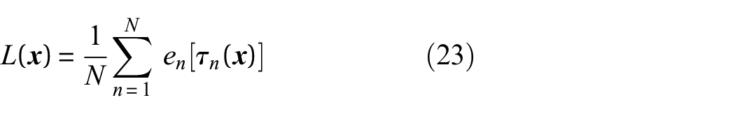
If the acceptable detection performance of critical damage is achieved in Level 2, damage localisation performance is quantified at Level 3. Two approaches to quantify localisation capability are proposed. The first approach considers a number of localisation estimates of the critical defects and quantifies the trueness (how close is the average estimation to the true location) and precision (the deviation among the estimations). Another approach is to quantify the localisation performance by providing reliability measure of the localisation estimates in various critical areas of the structure, that is, the true location of the defect is in a certain area given the estimation is in this area, which is achieved with Gaussian kernel distribution estimation and Bayesian inference.
The methodologies used in each level of quantification are presented in the following subsections.
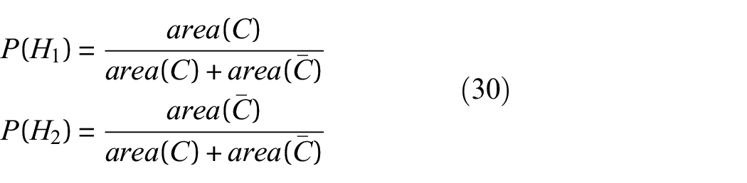
Level 0: optimal sensor placement
Given a CFRP airframe structure and its critical impact scenarios, a guided-wave SHM system can be designed to identify the impact damage while maintaining a reasonable cost. The amount of sensor implemented is a prime factor to GWSHM system implementation and in-service costs, and it’s a key constrain to GWSHM system design.
Thiene at al. 24 proposed a sensor placement method to achieve the maximum area coverage with a fixed number of piezoelectric sensors. A fitness function was introduced as an indicative measure of damage detection capability of a sensor network placement. A genetic algorithm (GA) is applied to find the optimal sensor placement based on the fitness function. This method is adopted in Level 0 and is introduced as follows.
The fitness function of sensor placement considers geometrical constraints and physical constraints.
Geometrical constraints include the following:
1. The detectability distribution of a sensor pair adding value 1 (
2. Minimising boundary reflections. To determine if a transducer pair should have a positive contribution to the overall fitness function, a threshold
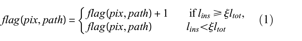
Boundary reflection coefficient
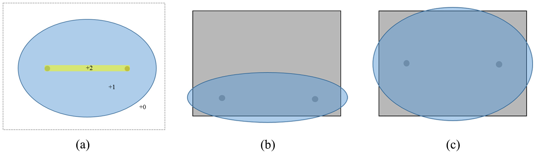
3. Disruption of guided-wave propagation path by openings. Wave propagation would be interrupted and the incident wave cannot be evaluated based on the direct distance between the transducers and the pixel if opening presents in any of the following positions, as shown in Figure 3.
Effective coverage area of a sensor pair (a) with added coverage value on the direct sight, (b) close to the boundary of the panel and (c) far from the boundary of the panel.
Disruption of wave propagation by openings: direct path between (a) actuator or (b) sensor; (c) path between the actuator and pixel; (d) path between the pixel and the sensor.
The global coverage of the sensor network is obtained by summing the values produced by each transducer pair as
The physical constraints of the fitness function of sensor placement lie within the guided-wave attenuation and frequency. It is known that the attenuation of guided waves is dependent on the excitation frequency. It is also assumed that the minimum detectable damage size is related to the excitation frequency through the wavelength of the guided wave. Therefore, the physical constraints are expressed as the frequency factor

where A and B are the two coefficients of the exponential trendline related to the selected actuation frequency.
The fitness function is determined by fusing the values from all the transducer paths and summing for all the pixels to obtain a single coefficient as
It is assumed that the best performance of the transducers network is reached when the fitness function is maximised.
Level 1: quantification of noise under EOC
Novelty detection has been a popular unsupervised approach for machine condition monitoring and used by a number of authors in guided wave-based structural damage detection, as only data from healthy or pristine structures are required to establish damage detection criteria.25–29 Novelty detection approaches generally involve extracting damage-sensitive features, establishing damage indices through feature fusion and threshold setting.
As GWSHM system is designed to be operating on the structure without major disruption of aircraft service, guided-wave measurements are likely to be recorded on an operating aircraft in varying EOC, and hence contain a significant level of noise that might greatly comprise the damage detection performance. It is a crucial step to quantify the uncertainty of damage-sensitive features in a pristine structure under the designed EOC for threshold setting to achieve reliable damage detection.
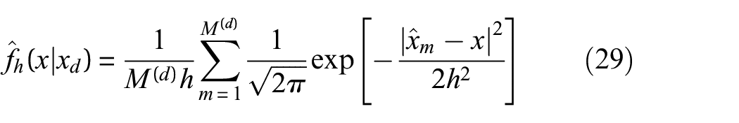
In this work, damage detection is considered as a novelty detection problem. The damage-sensitive features from sensor pairs are extracted and fused according to the sensor coverage distribution. The global distribution of fused features is used as a GDI and its threshold is derived from the noise level in damage-sensitive features under pristine condition.
Sensor coverage
A key aspect to be considered in establishing a GDI is the guided wave coverage area. To achieve reliable guided wave inspection of a large and complicated structure, a dense sensor network is usually implemented to cover the structure with effective diagnostic guided waves from multiple propagation directions to increase the change of capturing damage. A large number of the damage-sensitive features are obtained from the dense sensor network and they contain common information due to the overlapping guided wave propagating region. The fusion of the damage-sensitive features should consequently consider guided wave coverage distribution.
Having determined the optimal sensor placement in Level 0, the corresponding sensor coverage on the target structure can be obtained using equation (2). Figure 4 shows the sensor coverage in a simple flat panel with an eight-sensor network.
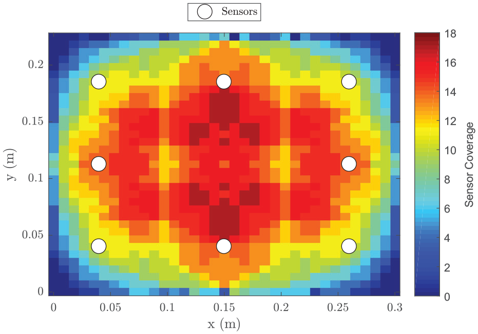
Sensor coverage of an eight-sensor network.
Sensor coverage is an indicative measurement of the probability of capturing damage, that is, the more effective guided wave paths available at a location, the more likely damage at this location can be captured. However, this is under the assumption that guided waves are only affected by the occurrence of damage. In a real application scenario, guided wave signals are likely to be acquired in various EOC. The difference in a current signal and a baseline signal is no longer only caused by the occurrence of damage but also by a difference in the measurement condition. In this case, sensor coverage is not sufficient to describe the damage detection capability of a sensor network. The variation in damage-sensitive signal features in the intended EOC must be quantified to achieve reliable damage detection.
Damage-sensitive signal feature
Guided waves are dispersive in nature, but for a certain frequency and plate thickness, the two fundamental guided wave modes, A0 and S0, are nearly non-dispersive. The non-dispersive guided wave response is achieved by frequency selection. Signal response to tone-burst signals at selected frequencies is recorded for a sensor network under the pre-defined EOC. Denoting the mth recoding of the signal with sensor pair i as

where
where
where
where
Let

The magnitude of the residual signal is obtained using Hilbert transform as


The time position of the peak residual envelop is
Assume,
Feature fusion and threshold setting
Two feature fusion and threshold setting methods are presented and discussed here: (1) sensor pairwise-based damage detection and (2) spatial damage indices-based damage detection.
Sensor pairwise-based damage detection
Sensor pairwise detection is the simplest approach and is commonly adopted in the literature,7,29,30 especially for one pair of sensors. The damage-sensitive features from each individual sensor pair are used to create an damage index for that sensor pair. As the mean and standard deviation of the damage-sensitive features in pristine state are known from equations (13) and (14), the upper bound of the feature value from sensor pair i in pristine state can be calculated and serves as the damage detection threshold

where
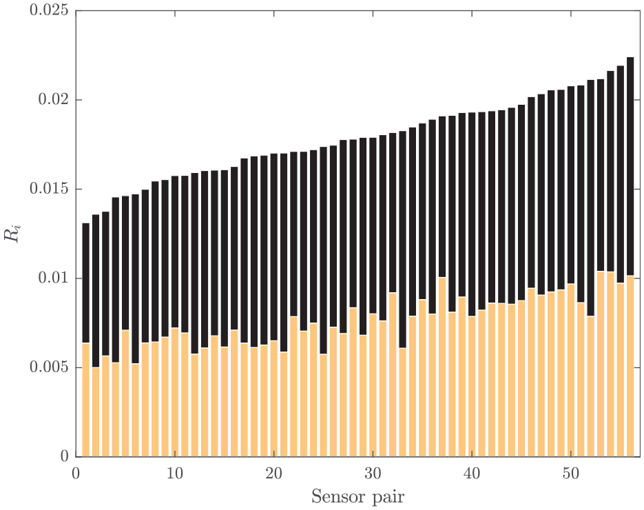
The upper bound of 56 damage-sensitive features in pristine state. The yellow bar represents the value of
However, in large and complex structures, a large network of sensors is required for adequate damage detection capability and high sensor coverage for critical locations. A drawback of sensor pairwise detection is that it might result in ambiguous global damage detection result due to inconsistent damage indication from different sensor paths. This approach also ignores information regarding the spatial position of sensor pairs and their common coverage area. This is particularly important in a dense sensor network.
Spatial damage indices-based damage detection
A damage detection strategy that considers spatial sensor placement is proposed. The damage-sensitive features from all sensor pairs in the sensor network are fused according to the coverage area to derive spatially distributed damage indices. A GDI is then determined based on the global feature of the spatial damage indices. A threshold of the GDI for damage detection can be determined according to the variability of the GDI when no damage is present.
Sensor network coverage-based feature fusion
The damage-sensitive features extracted from all signal paths are fused according to the sensor coverage to derive a damage index based on the spatial distribution of the sensors.
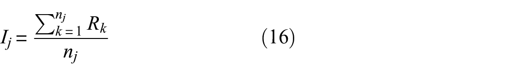
To fuse signal features based on sensor network coverage, the structure is partitioned into J pixels and the assigned value to each pixel is included in the spatial damage index vector
where
When signal features are averaged as in equation (18) at their mutual pixel location, the variance of the averaged signal features is reduced.
Spatial distribution of the expected value of spatial damage index
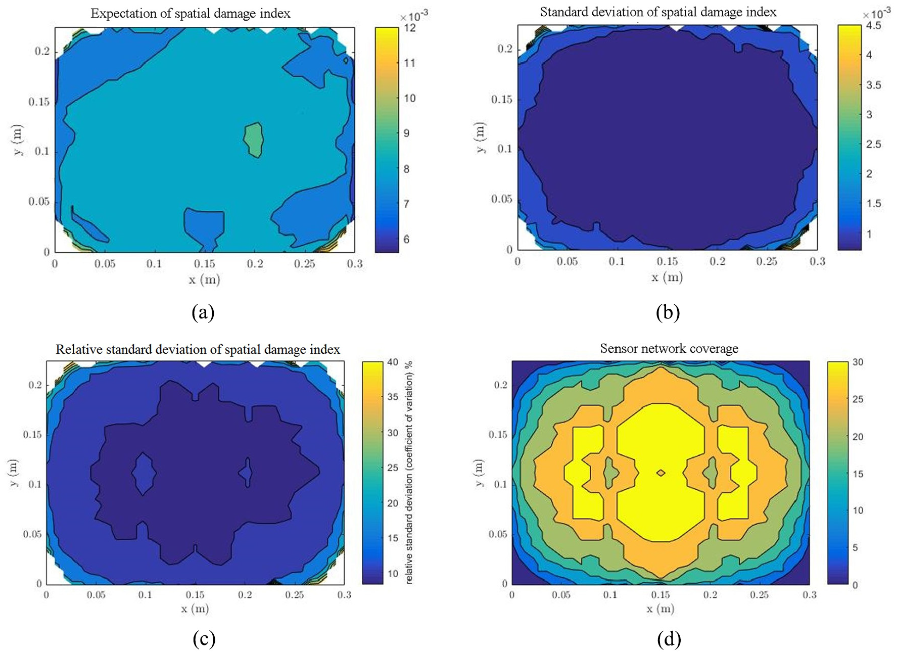
Spatial distribution of (a) expectation of the spatial damage index
Threshold setting
To decide whether the damage is present in the structure, detection criteria are established for the spatially distributed damage index considering the uncertainty from a range of pre-defined EOC.
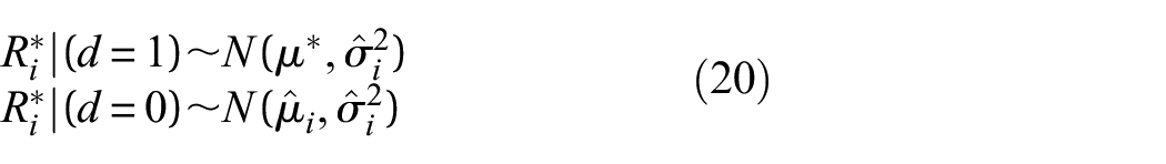
Let d and
If the spatial damage indices of an unknown state deviate from the value range at the pristine state with variation caused by varying EOC, it is considered that the damage is present in the structure.
The spatial damage index value represents the likelihood of damage presence at the spatial location. A spatial damage index value at the pristine state is

where
For damage detection within a designed sensor coverage area, the global value of the spatial damage index vector I is considered. In the conventional ROC approach, the threshold is swept over the range of feature values,
16
which does not provide a practical way of threshold setting. Here, the detection threshold is set at a percentile position of the spatial damage index vector
As an intuitive attempt, a threshold
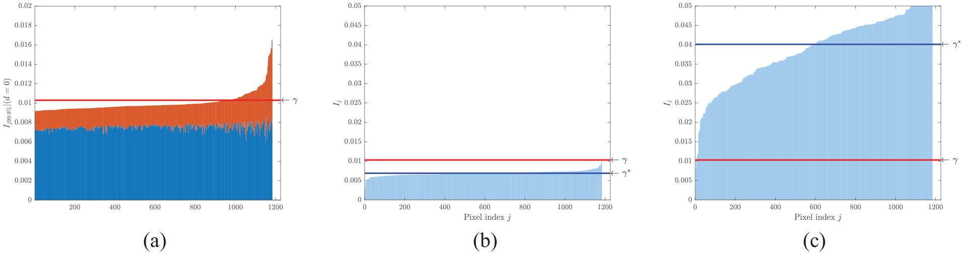
Damage detection criteria. (a) Threshold setting for damage detection. The orange bars indicate
For a structure whose integrity state is known, its spatial damage index vector, denoted as
Level 2: quantification of damage detection capability
Illustrative model for damage detection
An illustrative damage model is developed to demonstrate the damage detection process and highlight the influential factors. The model considers damage located at a certain position on the target structure. The size of the damage is neglected for simplicity. It is assumed that the damage-sensitive features of a signal increase to a certain level if sensor coverage area contains the assumed damage position.
Assume, the damage occurs at a location denotes all signal features by *. Let
The spatial damage index
Figure 8 presents the distribution of the spatial damage index value obtained with the model. Two damage severity levels are considered by assuming the damage-sensitive signal feature to increase to 0.02 and 0.04, presented in Figure 8(b) and (c), respectively. For each damage severity, damage at a low sensor coverage position and a high sensor coverage position is considered. It can be seen that the damage at positions with high sensor coverage results in greater GDI, thus the damage is more likely to be detected
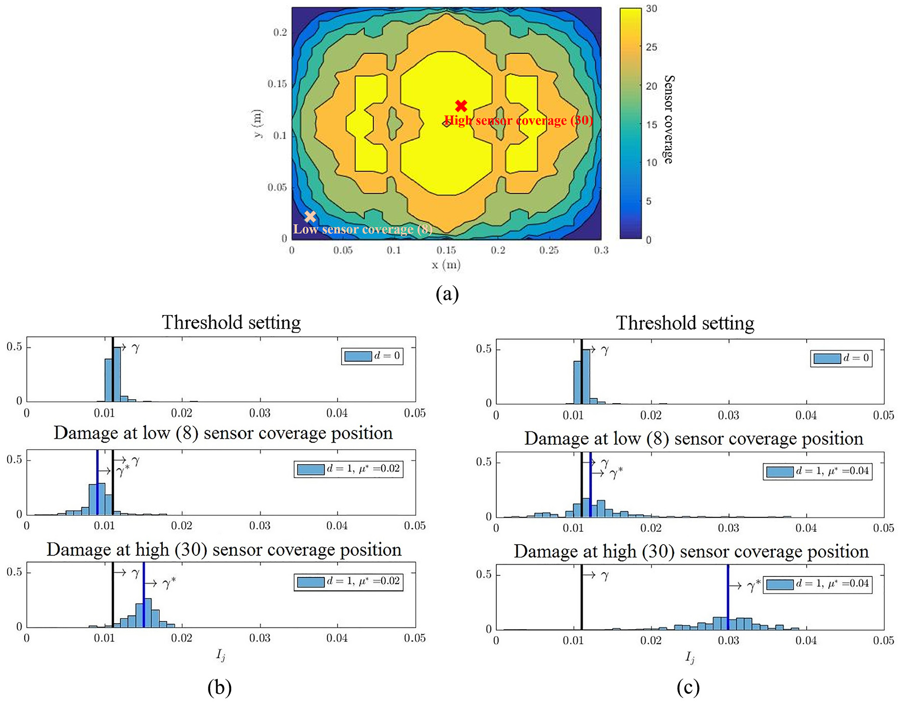
Demonstration of damage detection with an illustrative model. (a) Sensor coverage distribution of the sensor network. The red cross marks the damage location at high (30) sensor coverage position, the pink cross marks the damage location at low (8) sensor coverage position. (b) Low damage severity. (c) High damage severity.
Alternative detection sensitivity can be achieved by evaluating the different values of the threshold
Redundancy of a sensor network
As demonstrated in Figure 8, good sensor coverage is critical for damage detection under the presence of uncertainties. As degradation or failure of sensors is unavoidable during long-term monitoring, a redundant design concept must be adopted for the reliable long-term service of a GWSHM system, that is, the sensor coverage in critical locations on the structure must be redundant.
The redundancy of a sensor network can be assessed by the sensor coverage under critical sensor loss. Critical sensor loss is determined as the sensor failure that leads to the most dramatic coverage reduction at the critical damage location. When critical sensor loss occurs, the sensor network coverage should still be sufficient for the target structure. Examples of redundant sensor network design are presented in Figure 9.
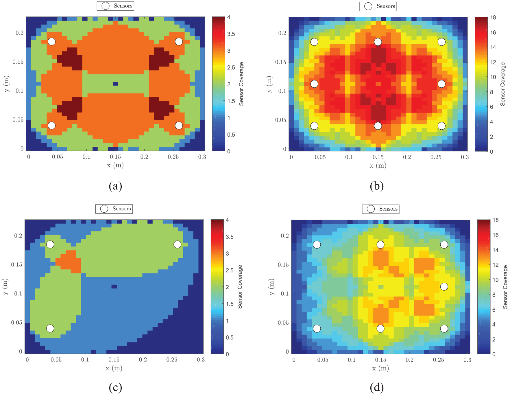
Sensor coverage of (a) four sensors, (b) eight sensors, (c) three sensors and (d) seven sensors.
Four-sensor network and eight-sensor network are two possible sensor network placements, as shown in Figure 9(a) and (b), respectively. Assuming one sensor is faulty and thus eliminated from the sensor network, the coverage of the four-sensor network is reduced from 3 to 0 near the faulty sensor location, as shown in Figure 9(c), which is not acceptable. The eight-sensor network, however, only suffer from coverage drop from 14 to 6 at the faulty sensor location, as shown in Figure 9(d), which is still sufficient for damage detection. Therefore, the eight-sensor network is considered more robust than the four-sensor network.
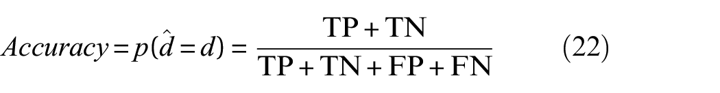
Detection performance evaluation
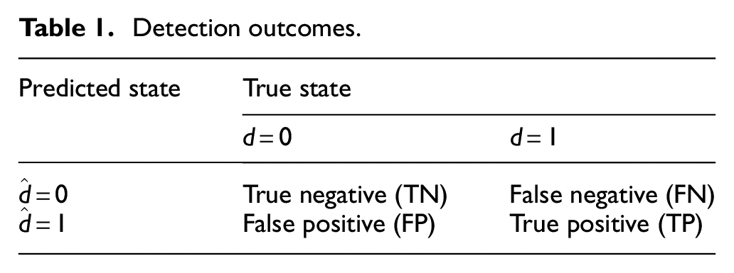
As discussed in the ‘Introduction’ section, hit/miss analysis is used for the reliability assessment in detecting BVID. Table 1 presents the four outcomes of damage detection.
Detection outcomes.
POD,
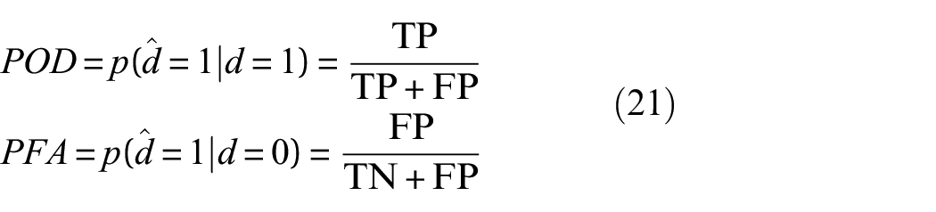
The ratio of correct predictions to the total number of predictions made,
Level 3: quantification of damage localisation capability
As a result of Level 2, the damage detection capability of a sensor network in the pre-defined EOC is quantified. For large-scale structures with critical positions where damage can significantly reduce the residual life of the structure, the location of the damage provides important information for complimentary localised non-destructive inspection and maintenance actions. Therefore, in Level 3, approaches to quantify damage localisation capability are proposed.
In this work, a commonly used imaging method in the literature, DAS, is used for damage localisation. Other damage imagining methods can be applied and assessed in a similar manner.
DAS method is well documented in a number of publications. For the completeness of this work, a brief description is given here. In the DAS method, the envelop of residual signals from each sensor pair,
where
Guided wave velocity is used to calculate the expected arrival time of scattered signal. The time delay is calculated as
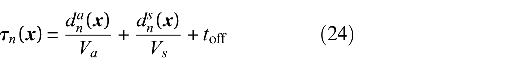
where
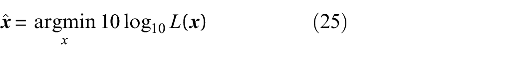
The spatial likelihood index is transformed to dB scale as
To suppress the effect of noise in the damage imaging process and damage location estimation, a two-step noise-suppressing technique is proposed.
A mean filter
A mean filter is used to suppress the sparse extreme values in the spatial likelihood indices which are unlikely to be the damage location. The spatial likelihood index
Application of a mean filter on the spatial likelihood index
Determine location estimate
The estimated damage location is usually determined at the location where the spatial likelihood index is the greatest. However, as the spatial likelihood index might be corrupted by noise and the maximum spatial likelihood location for the same damage may vary significantly, causing low precision in the location estimate. To eliminate the effect of noise, the damage location is estimated based on a group of possible location estimates.
Instead of taking the location estimate at which the spatial likelihood indices are the maximum, the locations whose spatial likelihood indices are among the top 1% are selected as possible locations with equal likelihood to be the actual damage. These locations are then represented by the smallest enclosing circle, and the centre of this circle is taken the estimated damage location, as shown in Figure 10(b).
Localisation performance evaluation approaches
The purposes of evaluating the damage localisation method are as follows:
To quantify the accuracy of the location estimates obtained from a certain localisation method
To provide practical guidance/reference for future maintenance decisions.
Two approaches are proposed accordingly to quantify the performance of the selected localisation method. The first approach is to quantify the accuracy of the location estimate of damage in a certain critical area on the structure. The second approach considers the damage locations in various zones on the target structure and uses statistical methods to derive the probability of correctly indicating damage in certain zones.
The two approaches are introduced as follows.
Accuracy of the location estimation of damage in critical locations
According to BS ISO 5725-1: accuracy of measurement methods and results,32,33 the accuracy of a measurement method can be quantified in terms of trueness and precision: ‘Trueness is the closeness of the mean of a set of measurement results to the actual (true) value and precision is the closeness of agreement among a set of results’. Two types of errors are normally present in a measurement process: random error and systematic error. Random error is caused by random noise and anunbiased simplification of the process. Systematic error is the result of incomprehensible modelling assumptions and inappropriate simplification. Precision is impaired by random error, while trueness is undermined by systematic error.
The trueness of the location estimate is calculated from a number of location estimates
The precision of the location estimate is calculated as the area of the ellipse representing the covariance matrix. The steps to derive precision are as follows:
Obtain the covariance matrix of
Find the largest and smallest eigenvalues: the largest variance
Determine the enclosing ellipse with 95% confidence level; find the critical value of the chi-square distribution corresponding to 95% confidence level with two-degree freedom, noted as
The precision of the location estimate is measured as the enclosing area of the ellipse
Probability of correctly indicating a defect within a certain zone
For structures with added complexity, such as stiffeners and openings, the mechanical performance of the structure might be significantly impaired by the defects at certain locations, such as the foot of stiffener or corner of an opening. Accurate localisation of the defects in these locations is crucial to condition-based maintenance of such structures as they represent the worst-case scenario.
A two-step approach for estimating the probability of correctly indicating the defects within a certain zone is proposed. The first step is to derive the density distribution of the location estimates for a defect at various zones of the structure using Gaussian kernel density function estimation. The second step is to calculate the probability that the actual defect is in a certain zone when the location estimation falls inside this zone using Bayes’ law.
The approach is presented as follows:
Probability density distribution of the location estimates.
21
The target structure is partitioned into a grid of positions
where h is the kernel bandwidth.
Probability of correctly indicating damage in a critical zone. Divide the plate into critical zone C and non-critical zone
Two localisation results are the location estimation falls within the critical zone,
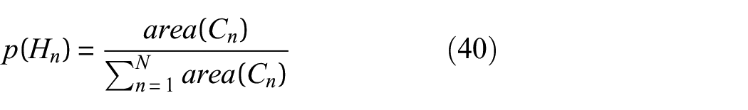
Prior probabilities of
The posterior probability that the actual damage location is in zone C when the location estimation falls in zone C is
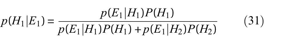
where likelihood
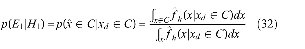
and
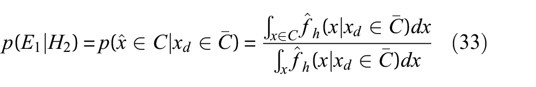
Likewise, the posterior probability of the actual damage is in zone
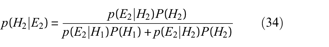
where
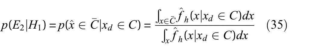
and

The approach above can also be expended for N zones on the structure,
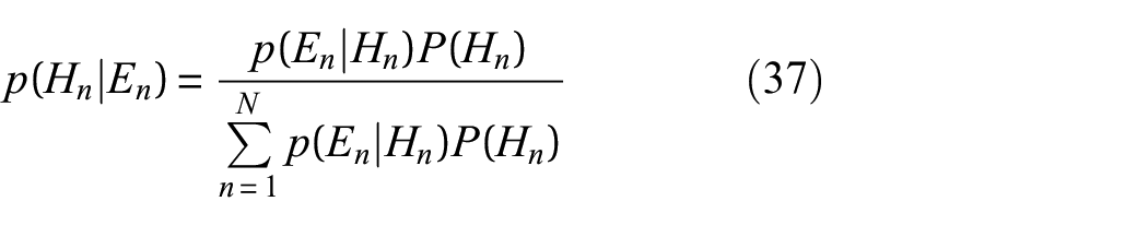
where
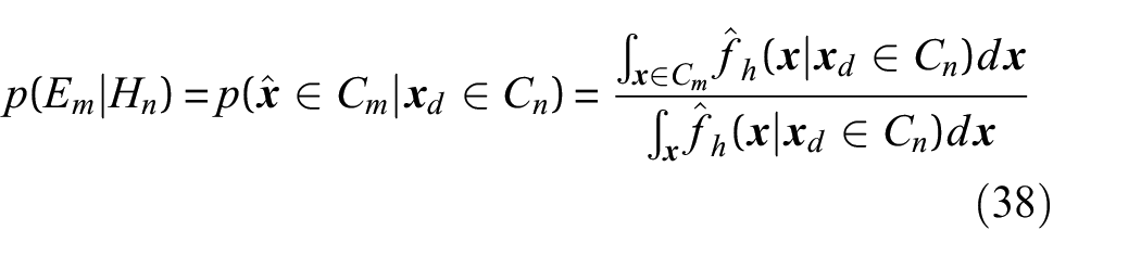
and prior probability of hypothesis
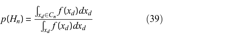
In the case of uniformly distributed damage occurrence,
Quantification of GWSHM on CFRP coupons
This section presents the quantification process of GWSHM on CFRP coupons up to size 500 × 250 mm2 in temperature controlled laboratory conditions. Temperature compensation of guided wave measurements was not necessary As the temperature variation was small (within 2°C). Temperature compensation method can be implemented for airframe structures in the case of greater temperature variation. 6
Simple flat panels (300 × 225 mm2) made from three types of CFRP composite materials are installed with piezoelectric sensors, and the performance of the GWSHM system is quantified following the proposed hierarchical approach. The materials and lay-up are presented in Table 2. The panels made from the first two materials are quasi-isotropic, whereas the panels made from the last material are anisotropic. The performance of the GWSHM system in a stiffened panel (500 × 250 mm2) made from M21/TS800 in Table 2 is also quantified and presented.
Material of flat plates specimens.
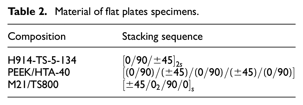
Quasi-isotropic unidirectional CFRP panel
A flat panel (300 × 225 mm2) is manufactured from unidirectional Hexply 914-TS-5-134 prepreg plies in the stacking sequence of
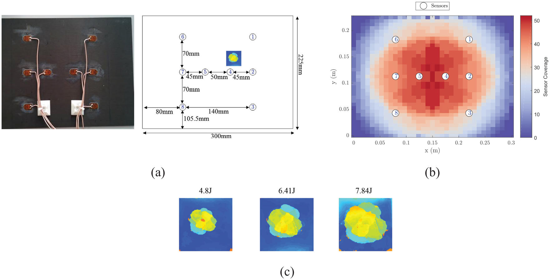
Quasi-isotropic unidirectional CFRP panel. (a) Sensor placement. (b) Coverage. (c) C-scan image of BVID after each impact event. The image size is 35 × 35 mm2.
Guided waves were excited with a five-cycle Hanning-windowed tone-burst at frequencies 50, 100, 150, 200, 250, 300 and 350 kHz. The highest amplitudes of the A0 wave mode and the S0 wave mode were observed in the sensor response to 50 and 300 kHz excitation, respectively.
BVID was introduced by the low velocity impact using an INSTRON CEAST 9350 drop tower. The panel was impacted at the same location three times with increasing energy of 4.8, 6.41 and 7.84 J. The formation of the BVID was confirmed using a handheld C-scan device (DolphiCam), as shown in Figure 11(c).
Before and after impact, guided wave measurements were collected 33 times from the sensor network on the panel in controlled laboratory conditions. The GDI
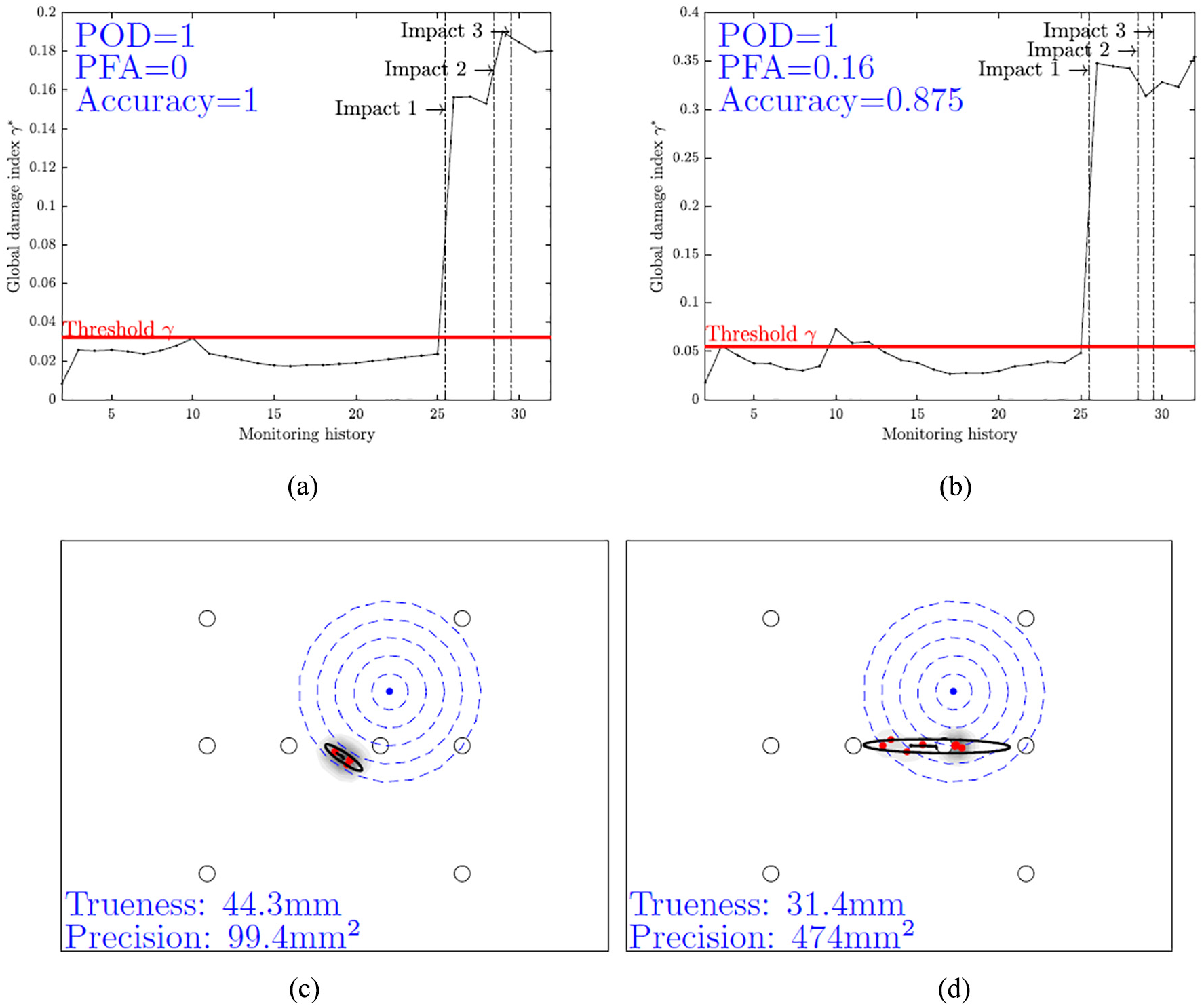
Damage identification results on the quasi-isotropic unidirectional CFRP panel. The monitoring history of the GDI
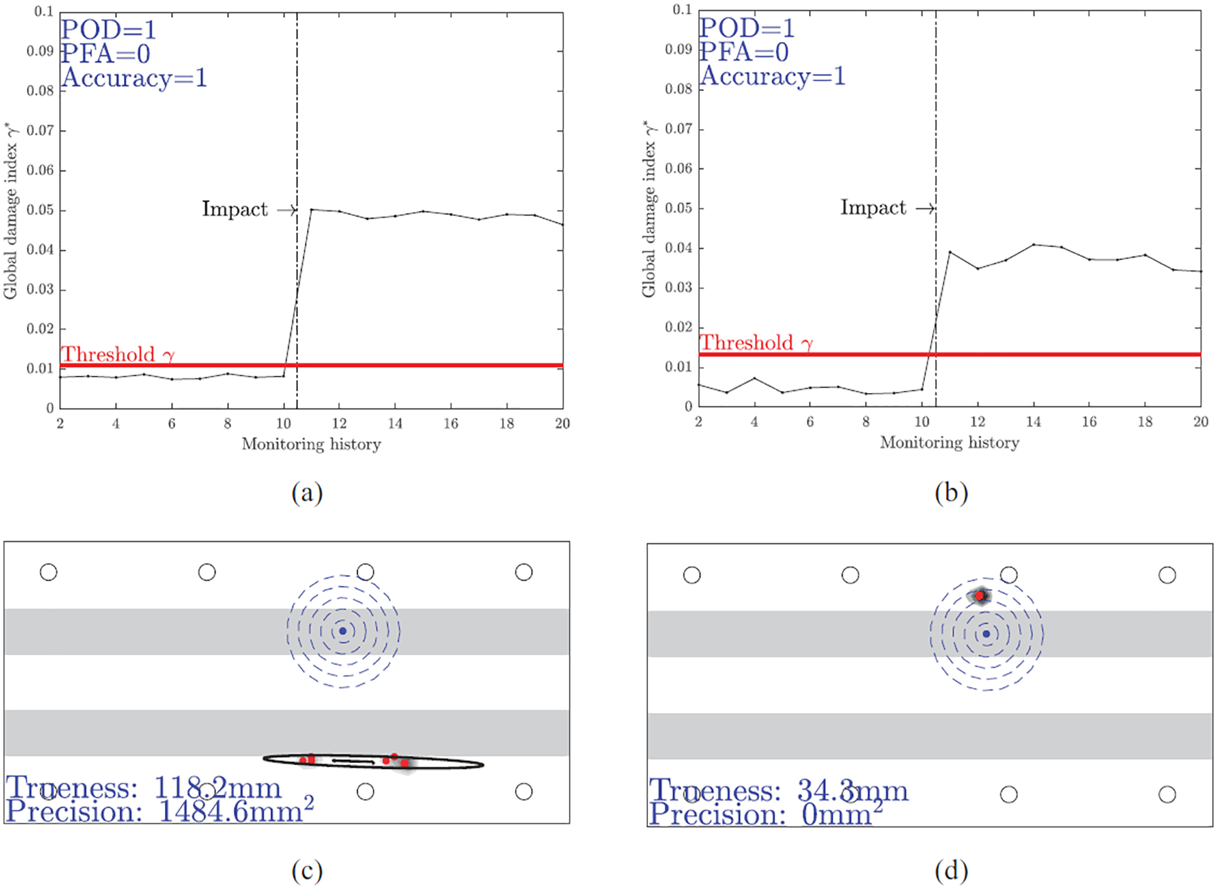
Damage detection performance is quantified using POD, PFA and accuracy as defined in equations (21) and (22) and is presented on the top left corner of the Figure 12(a) and (b). Guided waves at both 50 and 300 kHz are able to detect the occurrence of BVID with the predetermined threshold, POD = 1. However, at 300 kHz, damage that was incorrectly reported before damage was introduced, resulting in PFA = 0.16. Damage detection at 50 kHz showed better accuracy (accuracy = 1) compared to that at 300 kHz (accuracy = 0.875).
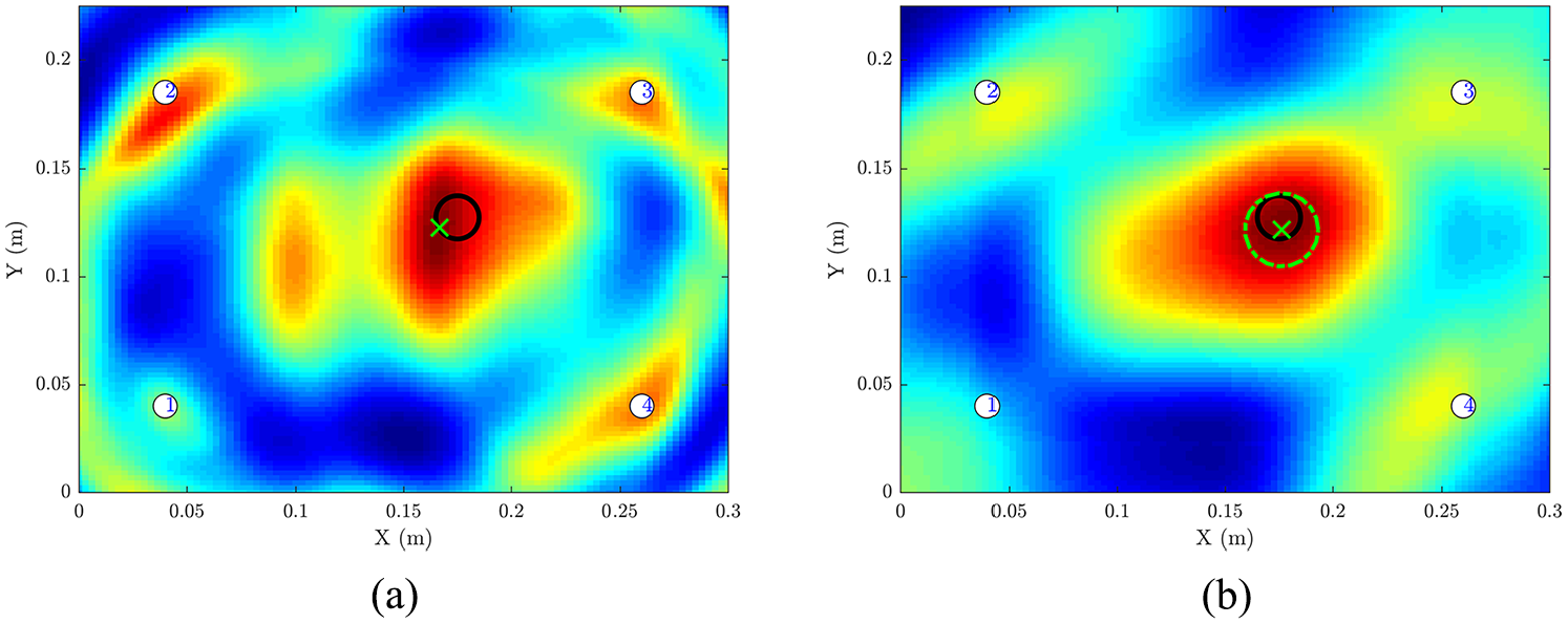
Damage localisation was performed for the positive detection cases, shown in Figure 12(a) and (b). Damage location was estimated using DAS at 50 and 300 kHz and the localisation results are presented in Figure 12(c) and (d). The impact location is marked by a blue dot surrounded by dash-line circles with radii from 10 to 50 mm for reference. The location estimates derived from each guided wave measurement are marked as red dots. The distribution area of the location estimates is represented using an ellipse centred at the mean coordinates of the estimates. The distance from impact location to the centre of the ellipse indicates the trueness of the estimations. The area of the ellipse represents the precision of the estimates. The value of trueness and precision is presented on the bottom left of each case. The trueness of estimates is around 33 mm.
Quasi-isotropic woven CFRP panel
A quasi-isotropic laminate (300 × 225 mm2) was made of woven fabric-reinforced thermoplastic (PEEK/HTA40) plies in the stacking sequence
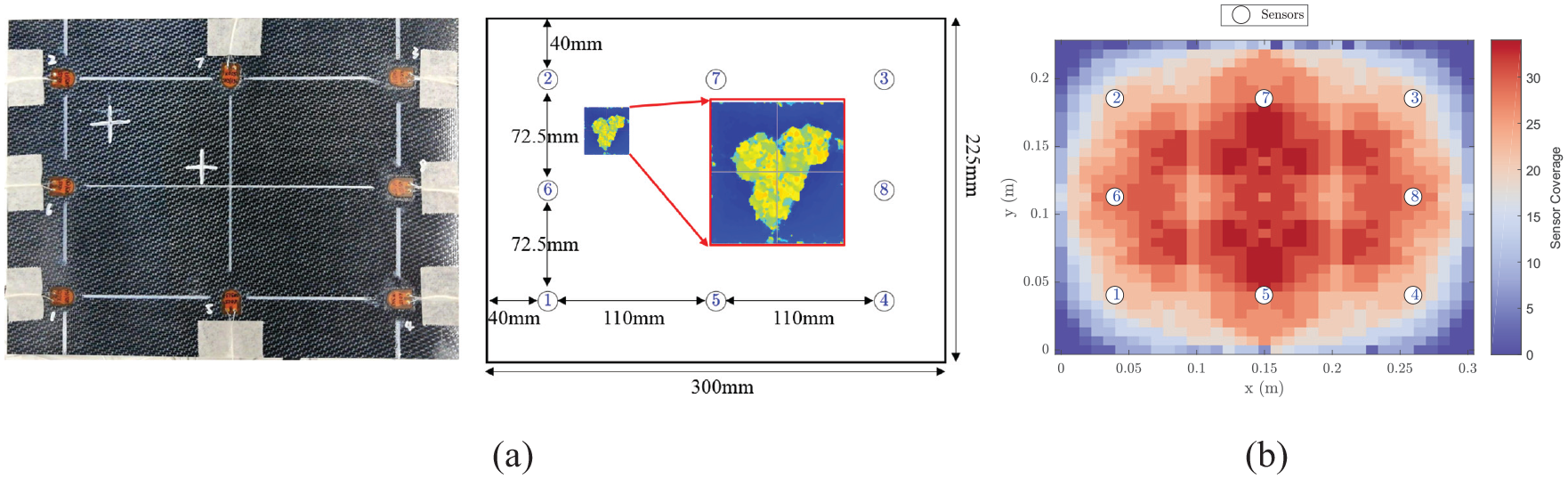
Quasi-isotropic woven CFRP panel. (a) Sensor placement. (b) Sensor coverage.
To improve the data acquisition speed, instead of exciting guided waves using a Hanning-windowed tone-burst signal centred at a single frequency, guided waves were excited using broadband linear chirp signals of frequency sweeping from 10 to 600 kHz over a 200-μs window. The recorded chirp signal responses were deconvoluted to Hanning-windowed tone-burst signals responses which are equivalent to the response of a guided wave to a tone-burst excitation. 35 The highest amplitudes of the A0 wave mode and S0 wave mode were observed in the sensor response to 50 and 250 kHz excitation.
BVID was introduced by low velocity impact using an INSTRON CEAST 9350 drop tower. The panel was impacted over a small region four times at 12 J, introducing BVID over an area of 200 × 200 mm2. The formation of the BVID was confirmed using a handheld C-scan device (DolphiCam), as shown in Figure 13(a).
Before and after impact, guided wave measurements were collected 100 times from the sensor network on the panel in controlled laboratory conditions. The GDI
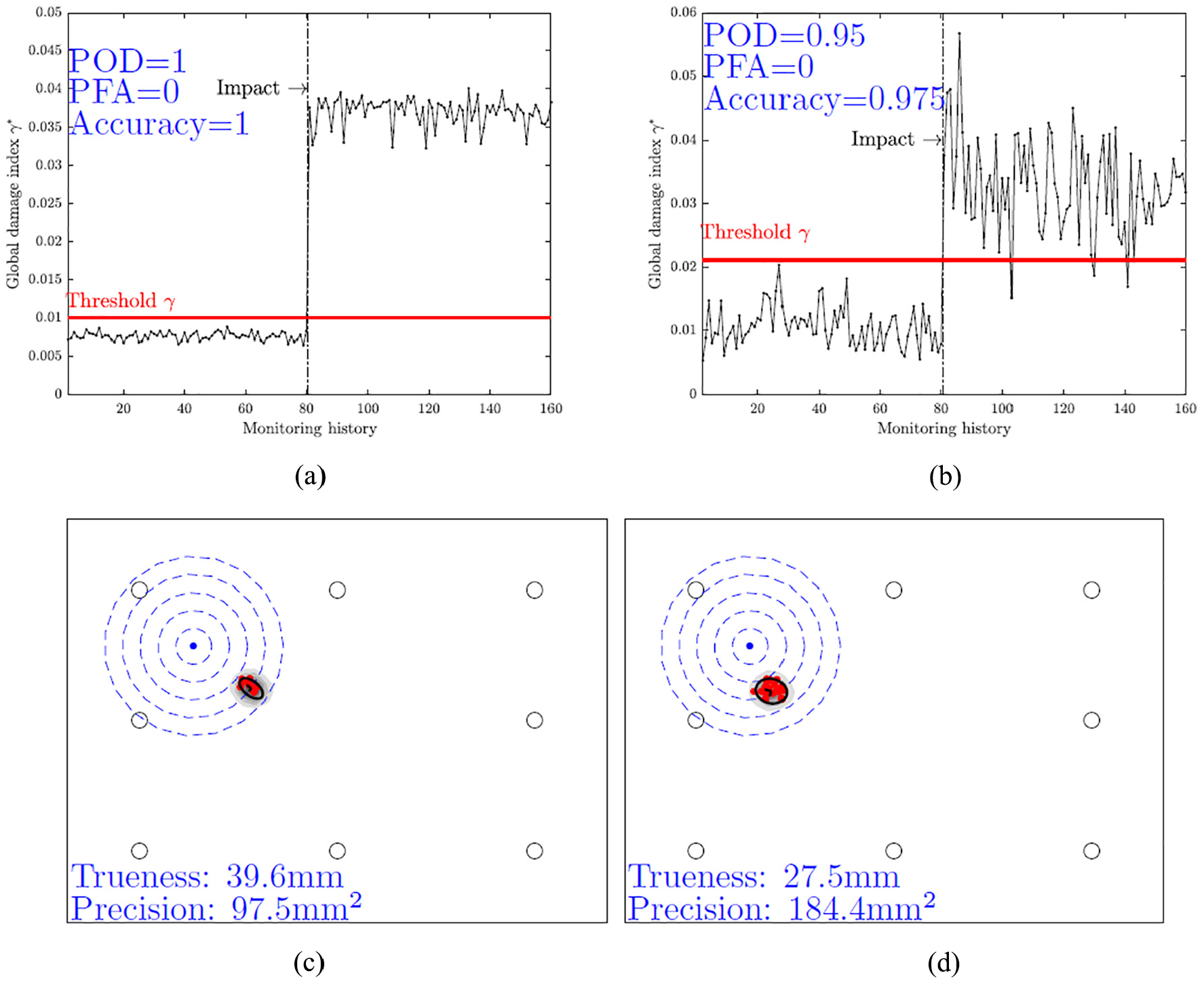
Damage identification results on the quasi-isotropic woven CFRP panel. Monitoring history of GDI
It can be seen that the GDI at 250 kHz fluctuated more than 50 kHz, indicating that the S0 wave mode is more prone to variation in environmental conditions than the A0 wave mode. Impact damage was successfully detected at 50 kHz with a detection accuracy of 1. Damage detection at 250 kHz resulted a few cases of false negatives, which led to POD of 0.95 and detection accuracy of 0.975. BVID was located using DAS at 50 and 250 kHz. The localisation results are presented in Figure 14(c) and (d). DAS using guided wave responses at 50 kHz provides the best trueness in the location estimates.
Anisotropic CFRP unidirectional laminate panels
Three 300 × 225 mm2 flat panels were manufactured from unidirectional M21/TS800 prepreg plies in the stacking sequence
Anisotropic unidirectional CFRP panel. (a) Sensor placement. (b) Sensor coverage. (c) C-scan images of BVID after each impact event on three panels. The zoomed in area is 35 × 35 mm2.
BVID was introduced by a 20-J low velocity impact using an INSTRON CEAST 9350 drop tower. The formation of the BVID was confirmed using a handheld C-scan device (DolphiCam). The location and energy of the impact events and C-scan of BVID on the three panels are shown in Figure 15(c). Before and after impact, guided wave signals were collected multiple times from the panel in controlled laboratory conditions. The GDI
Monitoring history of GDI
The history of the GDI
The detected damage is localised using DAS at 50 and 250 kHz. The damage localisation results in the three panels are presented in Figure 17. It can be seen that DAS using guided wave response at 50 kHz provides the most accurate location estimates of BVID.
Damage localisation results and performance quantification on three anisotropic unidirectional CFRP panels at 50 and 250 kHz.
A rectangular critical zone (140 × 65 mm2) is defined in the centre of the panel, as shown in 18.
Two out of three BVID locations are inside the critical zone. The location estimates of actual damage inside the rectangular critical zone are coloured in red. The location estimates of actual damage outside the rectangular critical zone are coloured in blue. The probability of correctly indicating damage within the critical zone is denoted as
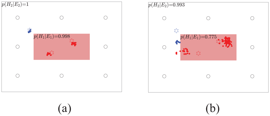
Probability of correctly indicating damage in a critical zone with guided waves at (a) 50 kHz and (b) 250 kHz.
Anisotropic unidirectional CFRP panel with an omega stiffener
A 500 × 250 mm2 flat panel with an omega-shaped stiffener was manufactured from unidirectional M21/TS800 prepreg plies in the stacking sequence of
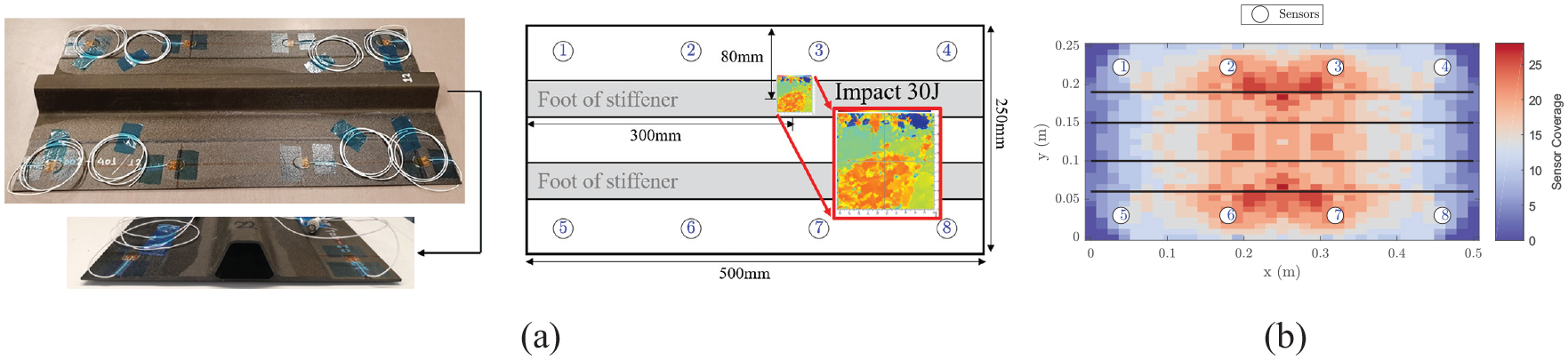
Anisotropic unidirectional CFRP panel with an omega stiffener. (a) Sensor placement. (b) Sensor coverage.
BVID was introduced by a 30-J impact at the foot of the stiffener, causing delamination of the skin and debonding between the foot of the stiffener and the skin, as shown in Figure 19(a). Before and after impact, guided wave signals were collected from the panel in controlled laboratory conditions. The GDI
Damage identification results on anisotropic unidirectional CFRP panel with omega stiffener. Monitoring history of GDI
The occurrence of the BVID in the stiffened panel was correctly detected at both frequencies with a detection accuracy of 1. Unlike in simple panels, the damage localisation estimation at 250 kHz is more accurate than that in 50 kHz, which might be the result of the S0 guided wave (250 kHz) being more sensitive to the surface damage, such as the debonding of the stiffener.
Quantification of GWSHM on CFRP components
This section presents the application and performance quantification of a GWSHM system on CFRP composite aircraft components in uncontrolled environmental conditions.
Experiment details
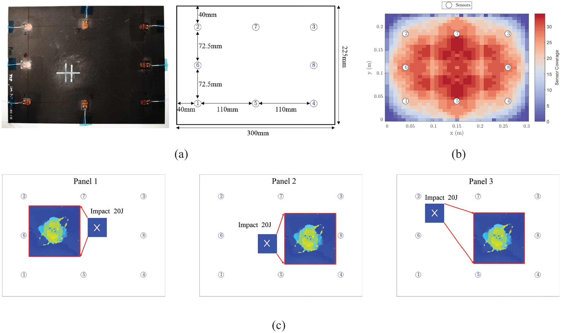
The components are flat anisotropic unidirectional CFRP panels installed with four CFRP omega stiffeners in the direction of the long side and three aluminium stringers in the direction of short side, as shown in Figure 21(a). Three identical components were manufactured. The skin and the omega stiffeners are made from unidirectional M21/TS800 prepreg plies in the stacking sequence of
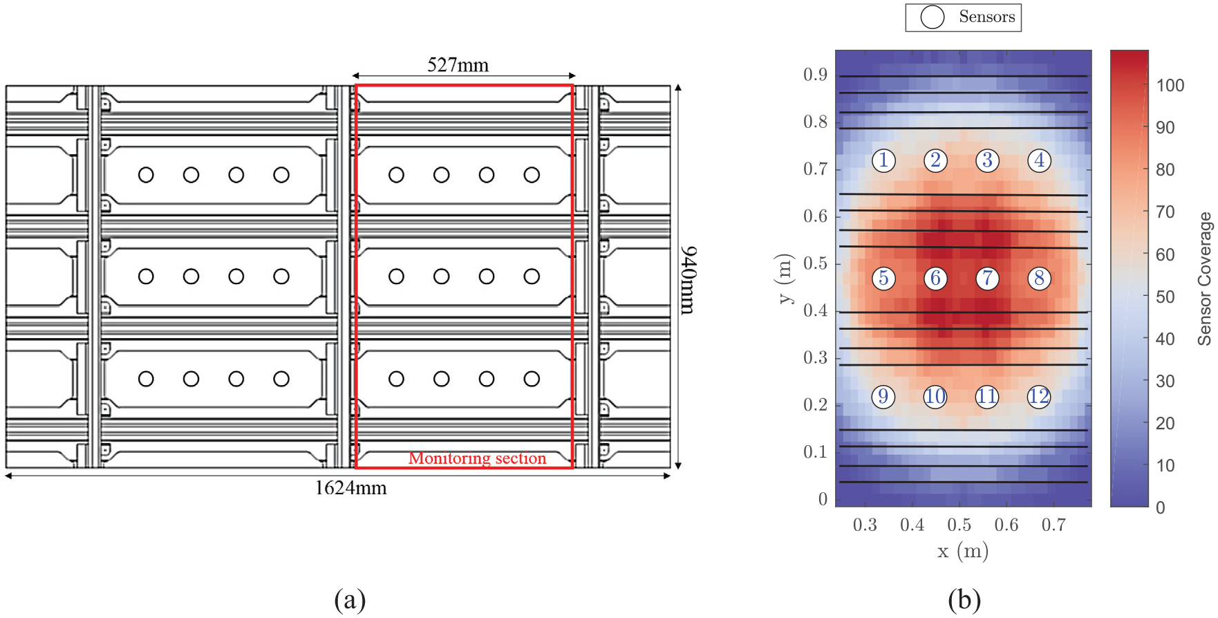
Flat stiffened panel with multiple stiffeners instrumented with DuraAct sensors. (a) Sensor placement. (b) Sensor network coverage of the highlighted monitoring section.
A total number of 24 piezoelectric sensors (DuraAct, PI ceramic) were bonded on the skin of the panel using thermoplastic film adhesive, 34 as shown in Figure 21. Considering the channel limitation (12 channels) of the signal acquisition setup and the influence of the vertical aluminium stringer, the panel was divided into two 527 × 940 mm2 monitoring sections separated by the middle vertical aluminium stringer with each area containing 12 sensors. The sensor network coverage on the monitoring section highlighted in Figure 21(a) is shown in Figure 21(b).
BVID was introduced by a low-velocity weight-drop impact with impactor mass of 5 kg. Two types of impact scenarios are considered: (a) impact on the outside of the panel during take-off by flying runway debris and (b) impact on the inside of the panel during maintenance by dropping heavy tools. The setup to simulate the two impact scenarios is shown in Figure 22. The formation of the BVID was confirmed using a handheld C-scan device (DolphiCam).
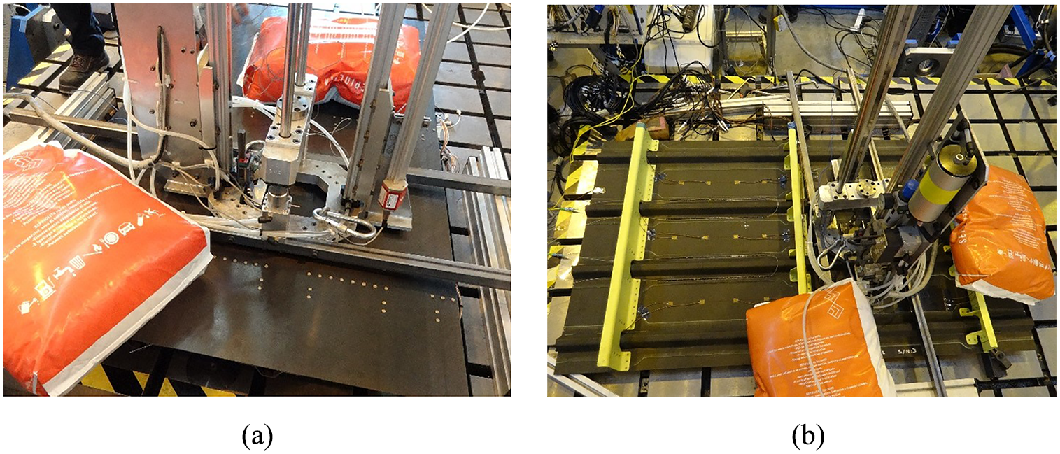
Impact setup. (a) Impact on the skin under the stiffener, simulating impact by runway debris. (b) Impact on the skin, simulating tool drop impact.
Panel 1 was impacted twice with 25 and 35 J at the same position on the skin under the foot of omega stiffener, causing delamination of the skin and debonding of the stiffener, as shown in Figure 23(a). Panel 2 was impacted three times at different locations, as shown in Figure 23(b). The first impact (20 J) was on the skin under the stiffener, causing delamination of the skin. The second impact (35 J) was on the skin between the feet of the stiffener, causing delamination of the skin and debonding of the stiffener. The third impact (20 J) was on the skin, causing delamination of the skin.
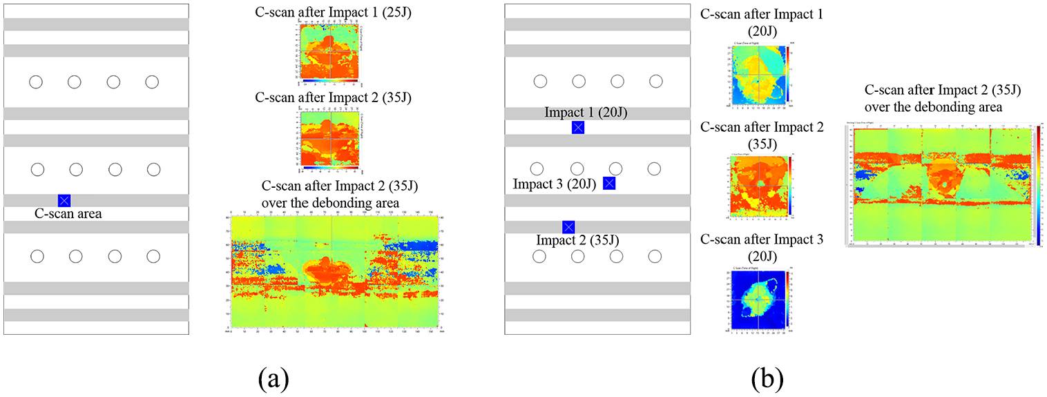
Impact location and C-scan after impact on (a) Panel 1 and (b) Panel 2.
Quantification of damage detection performance
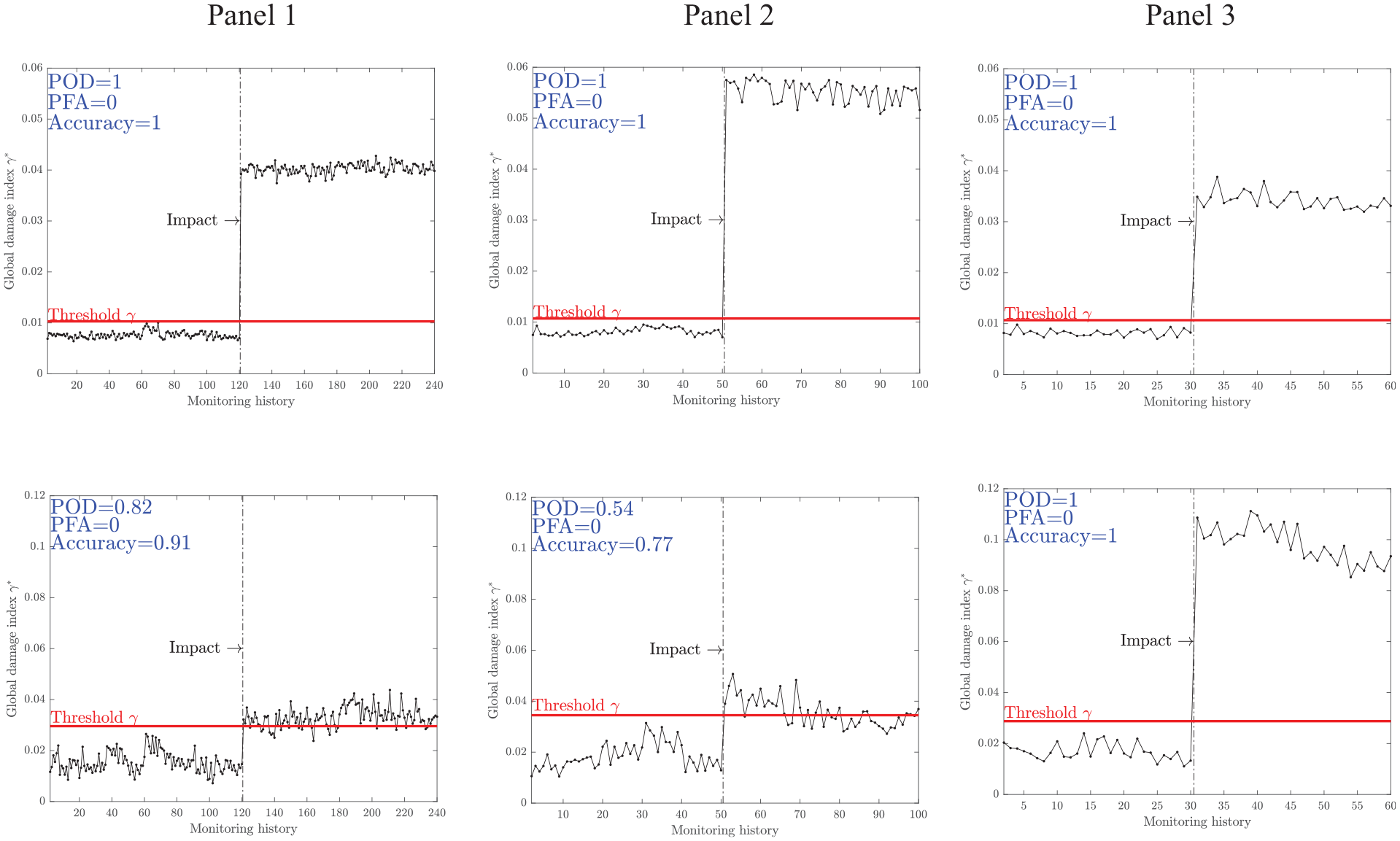
Before and after impact, guided wave signals were collected a number of times from the panel in an open plan laboratory with no means of temperature control. The history of GDI
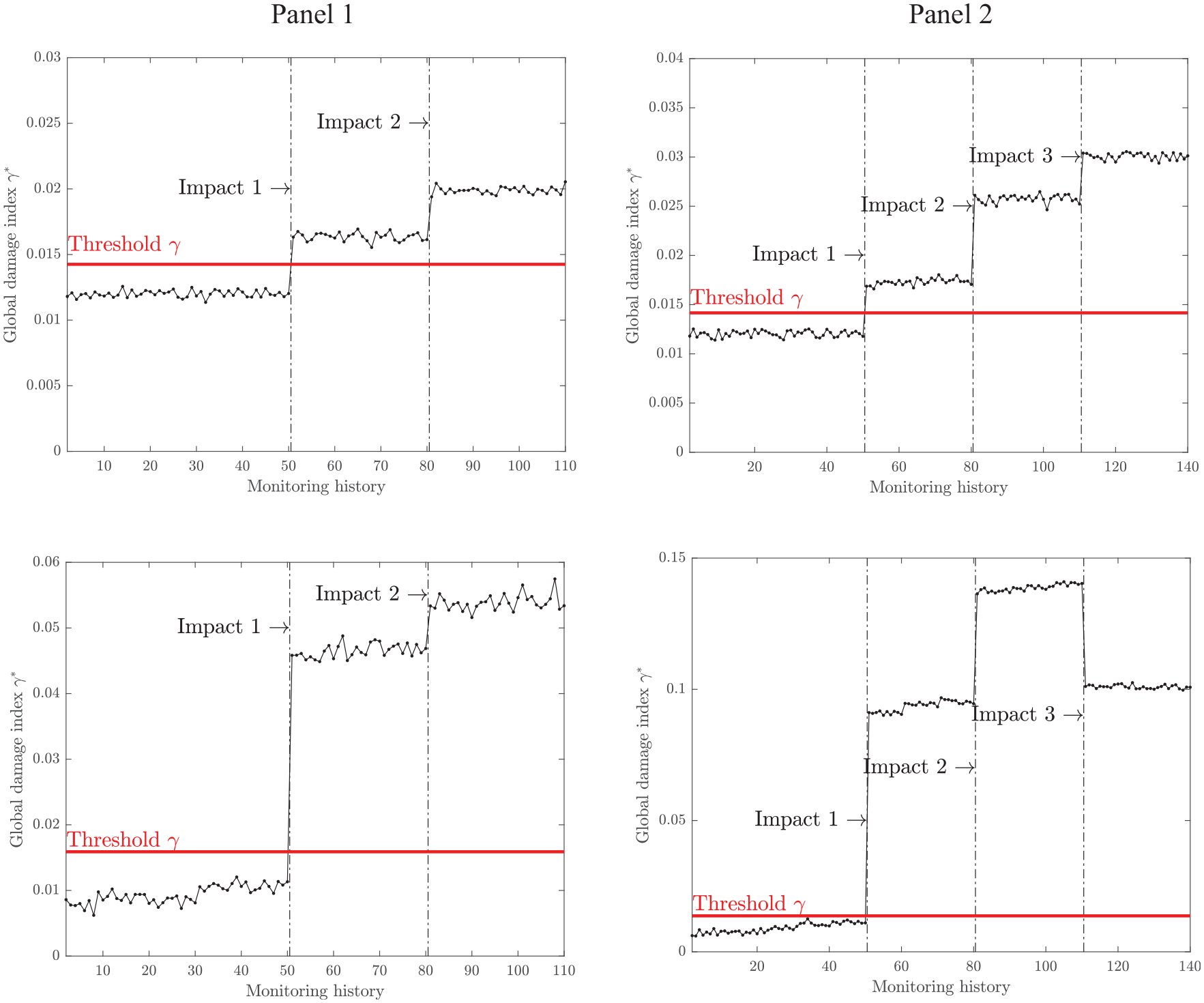
Monitoring history of GDI
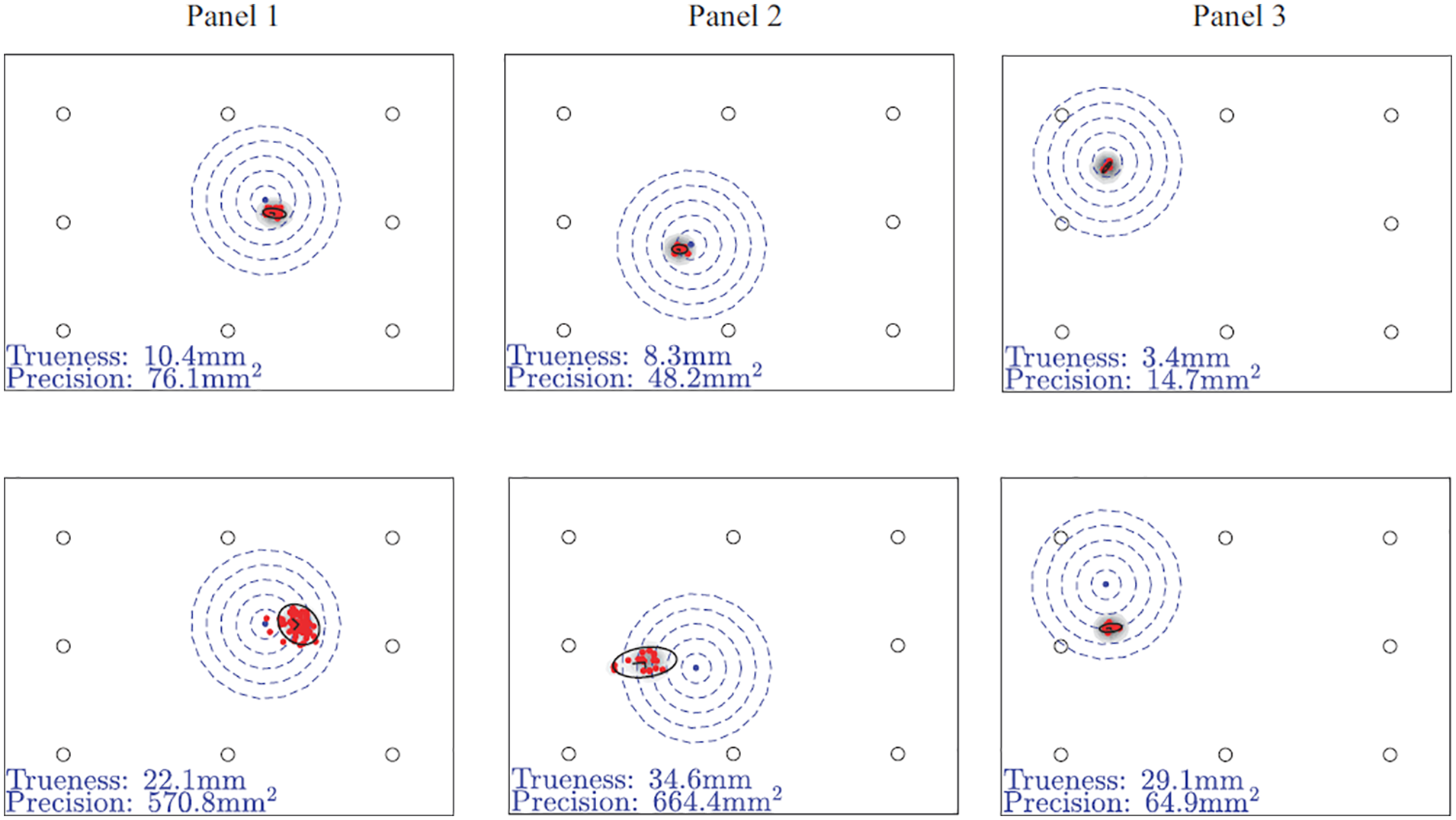
The GDI
Conclusion
This article proposes a multi-level hierarchical approach for establishing and assessing the performance of a GWSHM system for the detection and localisation of damage in CFRP composite structures. The hierarchical approach provides a systemic and practical way of establishing GWSHM systems for different structures in the presence of uncertainties and quantifies the system performance in four steps: (1) determining optimal sensor placement for the target structure, (2) threshold setting for a GDI derived from the sensor network based on the noise level in the intended EOC, (3) detecting damage in critical locations and quantifying the POD, PFA and detection accuracy and (4) locating the detected damage, quantifying the accuracy of location estimation and/or computing the probability of correctly indicating if the damage is present in the critical structural area.
The proposed approach was demonstrated for aircraft CFRP structures from coupon level (simple flat panels) to sub-component level (large flat panel with multiple CFRP stringers and aluminium frames). The detection and localisation of multiple BVID were performed in three types of CFRP materials.
Footnotes
Acknowledgements
The authors dedicate this work to a dear colleague, Ing Alfonso Apicella of Leonardo Aircraft, who passed away late last year. For many years, Alfonso had been instrumental in promoting new vistas of research within the European Aeronautics Community. They started working on SHM together in 2005 and this work is dedicated to his memory. The authors thank their colleague Llewellyn Morse for fruitful discussions related to Bayesian methods and for proofreading this article. They also thank the reviewers for their comments which have improved the article.
Declaration of conflicting interests
The author(s) declared no potential conflicts of interest with respect to the research, authorship, and/or publication of this article.
Funding
The author(s) disclosed receipt of the following financial support for the research, authorship, and/or publication of this article: This work was partially funded by the European JTI-CleanSky2 programme under the Structural Health Monitoring, Manufacturing and Repair Technologies for Life Management of Composite Fuselage (SHERLOC) project.