Detecting damage events in concrete using diffuse ultrasound structural health monitoring during strong environmental variations

Abstract

Diffuse ultrasonic wave measurements used in structural health monitoring applications can detect damage in concrete. However, the accuracy is very susceptible to environmental variations. In this study, a large concrete floor slab was monitored using diffuse wave fields that were generated by continuous-wave transmissions between ultrasonic transducers. The slab was monitored for several weeks while being subjected to changes in environmental conditions. Subsequently, it was damaged using impact hits, resulting in centimeter-scale cracking. The variations caused by the environment masked the effects of the damage in the measurements. To address this issue, the Mahalanobis distance was used to distinguish between the influence of the damage and the influence of the environmental variations. The Mahalanobis model uses amplitude and phase measurements of continuous waves at a set of different frequencies as inputs. A moving window approach was applied to the baseline data set to account for slow trends. This study shows that this technique greatly suppresses most of the variations caused by environmental conditions. All damage events in our data set have been detected.

Introduction

Structural health monitoring (SHM) systems that can continuously monitor the condition of concrete structures would help to address the ever increasing demand for safety and efficiency of civil structures, especially in light of the aging infrastructure in many countries. Unfortunately, it is far from trivial to implement SHM systems in concrete structures, due to their large sizes and the complexity of the material. Modal analysis is a useful tool for detecting damage from changes in global vibrational properties of the structure. However, these low-frequency methods are generally not able to detect small localized damages. Early detection of small cracks in concrete is important, as these cracks can quickly lead to more serious damages, for example, by exposing reinforcement bars to the environment. To localize these kinds of damages, higher frequency vibrations are necessary and ultrasonic methods can be employed. The use of ultrasonic methods in concrete is complicated since the aggregates and reinforcement bars inside the material are of a similar size as the wavelength of the mechanical waves. This leads to severe multiple scattering, which redistributes the energy from the directly propagating part of a transferred pulse to a diffuse wave field. When measuring a transient pulse traveling through concrete, these diffuse waves appear as a tail behind the direct propagating part of the wave. This trailing part of the wave is called the coda. It has been shown that proper analysis of coda waves, for example, by coda wave interferometry^1,2 (CWI), yields measurements which are much more sensitive to changes in the propagation material than any analysis of only the direct propagating wave by, for example, measuring time of flight. This high sensitivity is due to the multiple scattering of the late arriving waves; since they have longer travel times, they are more affected by changes in effective velocity than the direct propagating part. CWI is recently used quite often for non-destructive testing (NDT) or SHM purposes in concrete. We refer to the review article by Planés and Larose ³ for an overview.

The diffuse nature of high-frequency waves in concrete makes it impractical to implement different wave mode analyses, such as those used in metal plate structures, as the different dispersion modes are quickly concealed by the multiple scattered waves. However, one advantage of diffuse wave measurements is that they can be used to probe more than just the material located in a direct line between the transmitting and receiving transducers. This is because the multiple scattered waves traverse a wider region of the material. Thus, CWI could fill the gap between global, but insensitive, modal analysis methods and local, detailed NDT point measurements. This is a very promising prospect for SHM applications. The region of influence of diffuse waves between two transducers can be estimated by modeling the propagation of energy either as diffusion or using radiative transfer models.^1,4,5 These models can be used to construct sensitivity kernels that provide a spatial map of the sensitivity of the diffuse waves to changes in the material. These kernels have been shown to be complex, particularly if anisotropic scattering is considered, ⁶ but, in general, a high sensitivity region exists close to, and between, the transmitting and receiving transducers. These sensitivity kernels can be used in inversion procedures, such as the LOCADIFF algorithm, for locating local changes to the material.^7–11

In concrete, one issue with CWI and ultrasonic methods in general is the high attenuation of high-frequency waves, caused by both scattering and intrinsic absorption. This attenuation, combined with often noisy environments for civil structures, means that the transducers cannot be separated by large distance before the signal-to-noise ratio (SNR) decreases below useful levels. We have previously shown that for detecting bending damage in a concrete slab, the transmission of single-frequency, continuous waves and their sampling with a lock-in amplifier can produce data with similar sensitivity as transient CWI, but at much lower SNR levels. ¹² This allows larger distances to be used between transducers in a network, even in the presence of high-frequency noise. When a single frequency is transmitted continuously, a steady state is shortly reached that contains direct propagation, reflections from the boundaries, and scattered waves.

Localization methods such as LOCADIFF require measurements of transient time series, which are not available when measuring with a lock-in amplifier. Instead, we have earlier proposed a tomographic procedure that provides a rough localization of a small defect in a large concrete floor slab. ¹³ A similar method is used in this work.

One of the greatest challenges in SHM is the sensitivity of measurements to environmental or operational variations (EOVs). Examples of such conditions are temperature, humidity, wind, and traffic. EOVs can lead to false indications of damage in the structure and often affect measurements even more than the real damage. Unfortunately, the high sensitivity of coda waves also means that such methods are very susceptible to EOVs.^14,15

Some prior studies have used a reference specimen to compensate for measurement fluctuations in CWI measurements caused by temperature variations.^16,17 The reference specimen was subjected to the same temperature variations as the test specimen, but was not subjected to any loads. This thermal bias control technique worked well to remove undesired variations, particularly when it was combined with measurements of nonlinear parameters that are less sensitive to temperature variations. ¹⁸ Another method is the optimal baseline selection method (also known as the look-up table method), which stores a number of baseline data sets acquired at different environmental situations.^19–21 Each new measurement is then evaluated against the baseline with which it is most similar. This has been shown to work well with diffuse ultrasound measurements subjected to temperature variations. ²² Salvermoser et al. ²³ showed a strong correlation between velocity change and temperature, measured on a concrete bridge. Linear regression parameters could then be found which could be used to scale the measured temperature to estimate the effect on the velocity. By subtracting this estimated temperature-induced variation from the measured relative velocity change, only changes caused by damage should remain.

Unfortunately, a reference specimen will not always be available in real structures, and furthermore, most structures will be exposed to many EOVs other than global temperature variations. For instance, sunshine will occasionally heat some parts of a structure, while other sections remain cool. Exposure to EOVs will give rise to complicated behaviors, and statistical methods are needed for data normalization, possibly combined with a machine learning method. One popular tool for data normalization in SHM applications is the Mahalanobis ²⁴ distance. It has been used in a number of studies to successfully compensate for temperature variations and to detect outliers corresponding to damage.^25–27 Other data normalization methods exist, for example cointegration, and we refer to the book by Farrar and Worden ²¹ for more information on data normalization and machine learning approaches for handling EOVs in SHM.

For this work, a large concrete floor slab was monitored for several weeks while subjected to significant temperature variations and complex sunshine patterns. These changes occurred naturally due to the slab’s location in a laboratory hall with large windows. The monitoring system consisted of a distributed network of piezoelectric transducers which were used to transmit or receive continuous waves on command. The monitoring system is the same as used in our previously published work, ¹³ where it was shown to successfully detect damage in short-term acquisitions, where the data were not significantly affected by EOVs. The same localization procedure was applied here. A number of frequencies were used in order to increase the level of information yielded by each measurement cycle. Baseline measurements were gathered for more than 2 weeks before damage was introduced to the concrete. The purpose of this work is to demonstrate the use of the Mahalanobis distance as a data normalization procedure that can compensate for the influence of EOVs on diffuse wave field SHM measurements and to show that this enables the detection of a sudden damaging event.

Materials and equipment

Floor slab

The floor slab was an 8000 × 2110 × 80 mm composite concrete slab on top of glued, laminated timber beams (glulam). The concrete slab was reinforced with a steel mesh with a nominal diameter of 6 mm, and 150 mm squares. We refer to our previously published work ¹³ for more details of the geometry of the floor slab and the material composition of the concrete.

Ultrasonic transducers

Piezo ceramic disks (Ferroperm Pz 27) with 38 mm diameter and 10 mm thickness were used as ultrasonic transducers. The disks were glued to 25-mm-high aluminum cylinders. Bayonet Neill–Concelman (BNC) connectors were installed into threaded holes in the cylinders and connected to each pole of the ceramic disks. The transducers (lead zirconate titanate (PZT) disk and aluminum cylinder combined) have major resonant frequencies around 40–50 kHz, as well as some weaker resonances around 10–15 kHz.

Steel disks with 40 mm diameter and 5 mm thickness were glued onto the upper side of the concrete floor slab in a regular grid distribution. Each disk had a threaded hole for attaching the transducers. Eight transducers were used in this study. The layout and numbering of the transducers are shown in Figure 1.

Figure 1.

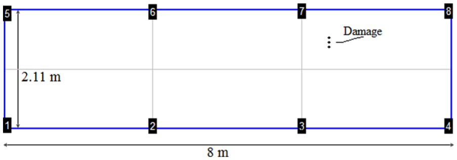
Layout and numbering of transducers and the location of the induced damage. The gray grid lines are those used in the tomographic procedure.

Measurement equipment

The excitation signal was generated by an Agilent 33500B waveform generator and amplified by an A.A. Lab Systems LTD A-303 amplifier. Measurements were performed with a Signal Recovery 7210 multichannel digital signal processing (DSP) lock-in amplifier that can measure up to 32 channels simultaneously. The lock-in amplifier outputs the amplitude of the measured signal and its phase relative to the driver signal (provided by the waveform generator).

A custom-made multiplexer from SubVision was used to switch the transmission and reception channels arbitrarily between the signal generator and the lock-in amplifier.

Experimental program

To obtain each measurement, one of the eight transducers was excited by a continuous sinusoidal wave with an amplitude of 60 Vpp. The signal started 100 ms before any measurements were made, providing sufficient time to reach a steady state. The lock-in amplifier measured the amplitude and phase at the seven transducers that were not transmitting. The multiplexer then switched to the next transducer in line to serve as the transmitter. The entire procedure was repeated at various frequencies: 13, 40, 42, 46, 48, and 50 kHz. These frequencies were chosen to correspond to the resonant frequencies of the transducers. The lowest frequency (13 kHz) was speculated to be less sensitive to damage than the higher frequency signals, but still sensitive to temperature variations. Low-frequency diffuse wave field measurements have been shown to be useful for measuring changes caused by variation in temperature. ¹⁴ Thus, they can be useful in the algorithm to differentiate between changes caused by damage and those caused by temperature.

In each measurement cycle, transmissions with all transducer combinations were repeated for each of the six frequencies, so that, in each cycle, 8 × 7 × 6 measurements were made. Each measurement cycle took approximately 1 min. This time can very likely be reduced by optimizing the control system. There was no external filtering or pre-amplification of the input signals to the lock-in amplifier.

The concrete floor slab was stored in a laboratory hall with windows covering one wall. This enabled the sun to shine into the laboratory, which heated the room considerably and resulted in day-night temperature cycles in the room with heterogeneous heating as the sunlight moved over the floor. Measurements were taken while the slab was left undamaged for 19 days. After that time, the concrete was locally damaged using a HILTI DX2 bolt gun with 6.8/11 M10 DX cartridges, power level “green” (“light”). The bolt gun was not loaded with bolts, but the piston was used to damage the concrete. The location of the damage is shown in Figure 1. Two shots were performed on the 20th day, and an additional shot was made a day later. After this, the floor was left undisturbed for several more days before the experiment was terminated, resulting in a total of 25 days of measurements. Figure 2 shows a photograph of the floor slab in the laboratory setting and a close view of the damage from the bolt gun impacts. The resulting damage consisted of small holes with surrounding cracked regions. The holes were 4–5 mm deep in the center, and the cracked regions ranged from 1 to 3 cm.

Figure 2.

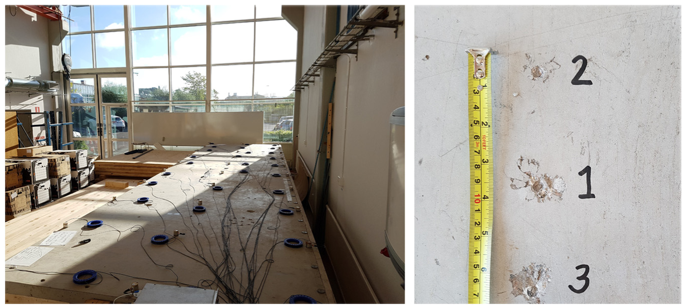
(Left) Photograph of the floor slab and the laboratory hall. Not all transducers seen in the photograph were used in this study. (Right) Close-up of the damage to the concrete. A ruler is included for reference.

Amplitude and phase measurements, as described above, were performed during the entire experiment at ∼35-min intervals. Two Velleman DVM171THD data loggers, placed on the floor slab, were used to log the temperature in the laboratory during the experiment, and the recorded temperature varied between 20°C and 27°C.

Data normalization

The lock-in amplifier measured the amplitude and phase of the steady-state wave field for each of the six frequencies at each receiver location. These can be viewed as 12-dimensional measurement points that have very complex behavior when subjected to changes in environmental conditions, such as temperature, or operational variations in the measurement system.

It can be very difficult to see trends in multivariate data or see deviations from previous system behaviors. One popular tool to evaluate such data is the Mahalanobis distance. A set of multivariate data points, the baseline, is used as a reference. Each new data point is evaluated as the distance between it and the center of the baseline data set. This distance is expressed as the number of standard deviations of the baseline in the direction, in multidimensional space, in which the new point is separated from the center. In this article, it is understood that “Mahalanobis distance” implies the Mahalanobis distance of the current sample to the baseline.

In this case, the amplitudes and phases of the six different frequency measurements are used as features in the Mahalanobis distance, and these define the dimensions in a 12-dimensional space. The general idea is that damage to the concrete will shift the measured data, in this space, in a direction that is orthogonal to the variations caused by, for example, temperature variations. Since this shift is in a direction where the baseline does not have a high variation, it will result in a relatively large Mahalanobis distance.

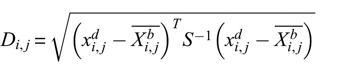
The following equation shows the calculation of Mahalanobis distance with transducer i as the transmitter and transducer j as the receiver

$$D_{i,j}=\sqrt{{\left(x_{i,j}^d-\overline{X_{i,j}^b}\right)}^T{S}^{-1}\left(x_{i,j}^d-\overline{X_{i,j}^b}\right)}$$

$x_{i,j}^d$ is a 12-dimensional six-frequency amplitude and phase measurement from the potentially damaged structure, $\overline{X_{i,j}^b}$ is the mean vector of the baseline data set, and $S$ is the baseline covariance matrix. Superscript T indicates a transpose.

The baseline consisted of 300 data points corresponding to measurements over approximately 1 week. If the baseline period is too short, even small variations in environmental conditions from day to day will result in large Mahalanobis distances. A week was deemed appropriate for the current experiment. However, apart from the daily variations in temperature, the floor and the transducers were also subjected to slow variations; for example, larger scale weather conditions changed approximately weekly. This led to the baseline becoming quickly outdated, which in turn led to an increasing Mahalanobis distance over time even though no damage was inflicted. To account for these slow variations, a moving window approach was implemented in which the baseline was continuously updated with new data points and old points were discarded. An example of a moving window algorithm was presented by Jeng, ²⁸ based on principal component analysis rather than the Mahalanobis distance.

Different results will be yielded depending on the “lag” of the baseline, that is, the time between the end of the baseline and the evaluated data point. In this implementation, no lag was introduced, so each measured data point was evaluated using a baseline consisting of the 300 previous points. This was well suited for sudden, instantaneous damage, as there was a sharp line dividing the subset of data from the non-damaged structure and the subset from the damaged structure. One effect of not using any lag was that the next sample (the second sample after the damage was introduced) was evaluated with a baseline which contained information that was also from the damaged structure. Therefore, the model learned this behavior and the point was given a low Mahalanobis distance. The result was that sudden damaging events appeared as sharp spikes in the timelines, even though the damage, of course, remained in the structure. Increasing the baseline lag smoothed the peak in time.

Localization

Since a continuous transmission, as mentioned previously, creates a diffuse field through wave scatterings and boundary reflections, all transducer pairs are potentially affected by changes in the concrete, not just those pairs whose direct propagation path exactly crosses the area of damage. As mentioned, the benefit of this is that the waves reaching the receiver will have traversed material for longer periods of time, which yields high sensitivity. It also means that a damaged region does not have to be located directly between two transducers to be detectable. The drawback is that it impedes spatial localization.

The influence of changes in the propagation material on diffuse waves is extremely difficult to predict. By modeling the diffuse propagation with either diffusion or radiative transfer models, it is possible to construct sensitivity kernels between a transmitter and a receiver.^4–6 These models confirm that the influence of a change on diffusely propagating waves is greater if the change is located close to either the transmitter or receiver or if it is somewhat in between the two. In a previous article, ¹³ the authors showed that a simple tomographic procedure can be used to provide rough localization of damage if a network of transducers is employed. In this procedure, the structure is divided by a grid. A value corresponding to the mean of the resulting Mahalanobis distance for all transducer pairs whose direct propagation path intersects the box is assigned to each grid cell.

Results and discussion

During the entire 25-day experiment, the temperature in the laboratory varied between 20°C and 27°C and sunshine heated both the floor slab and the transducers in complicated patterns. Figure 3 shows the measured temperature from one of the data loggers. It should be stressed that this temperature measurement only represents the temperature at one specific location on the floor slab; significant differences were noticed over the surface of the slab during sunny days due to the sun movement patterns. However, the temperature data in Figure 3 provide a good indication of the general temperature in the room at any given time, and 24-h cycles are clearly visible. The upper x-axis in Figure 3 displays the time in hours, and, for reference, the lower x-axis displays the corresponding sample numbers for the SHM system. The vertical gray lines indicate the times of the bolt gun shots.

Figure 3.

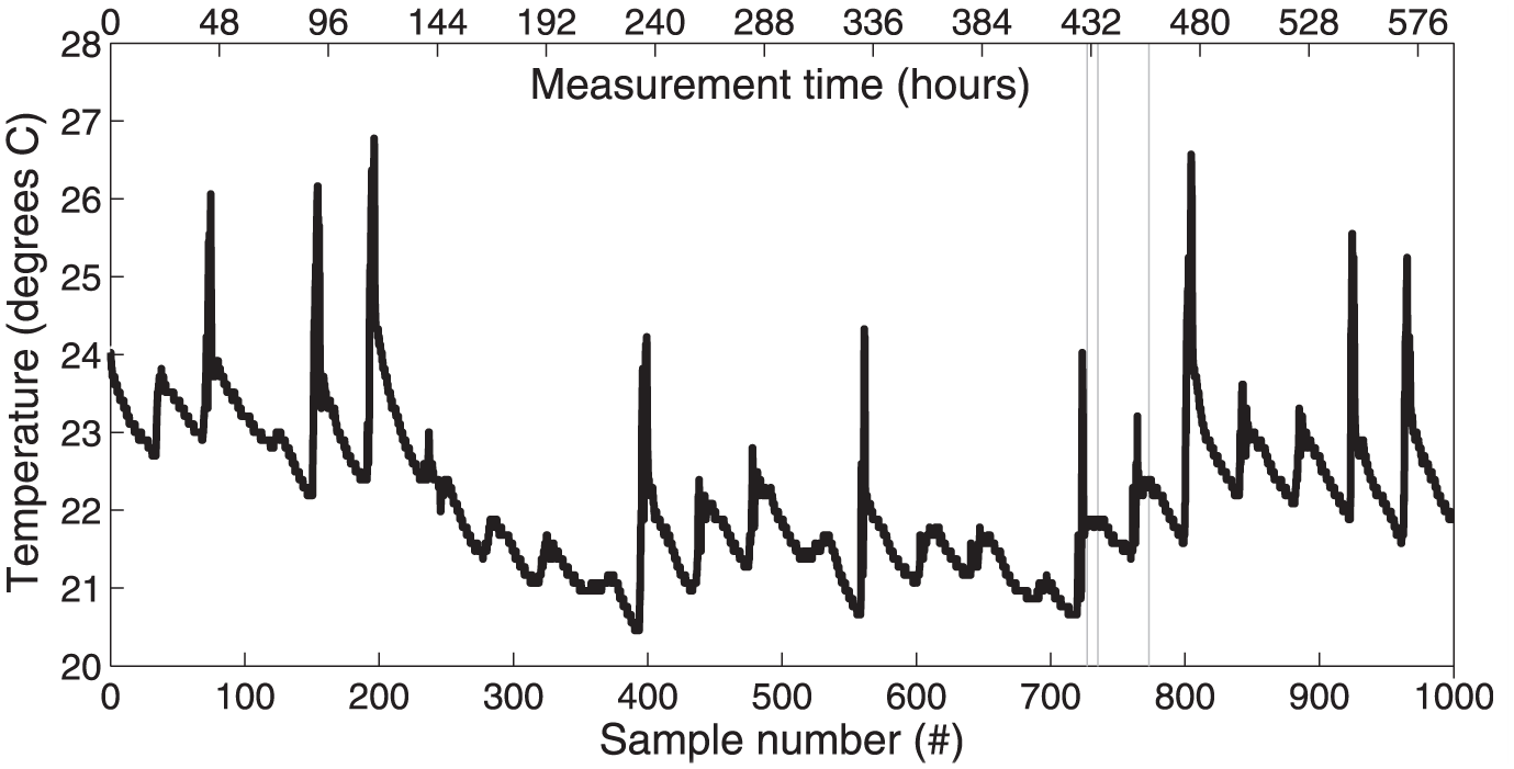
Temperature in the laboratory during the 25-day experiment. The gray vertical lines indicate the times of the damage events.

The effect of these variations can easily be seen in the raw data. Figure 4 shows example amplitude and phase data as a function of time (sample number) between transducers 7 and 3 for the 50 kHz signals. Similar data were acquired for every transducer pair combination and for each of the six chosen frequencies.

Figure 4.

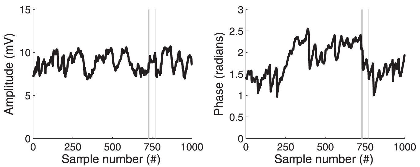
(left) Amplitude and (right) phase as a function of sample number for the frequency 50 kHz. Data are taken between transducers 7 and 3. The gray vertical lines indicate the times of the damage events.

As detailed above, impact hits were used to damage the concrete on the 20th day, just before samples 727 and 735, and once again on the next day, just before sample 773. The location of the damage is shown in Figure 1. The times of the shots are not obvious from the curves in Figure 4, as the fluctuations in the data due to environmental conditions obscure the damage events. In previous work, we have shown that similar damage can easily be detected with such 50-kHz continuous-wave measurements, viewing either amplitude or phase, in static environmental conditions. ¹³

The variations caused by the EOV are also illustrated in Figure 5(a) to (g), which shows the resulting images from the tomography procedure for a few select times using only the 50 kHz phase measurements. The gray scale corresponds to the deviations from the mean of the baseline data set, expressed in the number of standard deviations of the baseline set (averaged over the grid boxes in the tomography). This corresponds to a one-dimensional version of the Mahalanobis distance. The sample numbers 400, 600, 700, 727, 735, 773, and 805 are shown. False-positive indications are given at random times, as seen in Figure 5(a) to (c), and there is no noticeable difference before and after the damage. This illustrates the inability of the system to separate the effects of damage and EOV, when using only one of the measured parameter at a time. Similar results are yielded for any of the 12 measured parameters.

Figure 5.

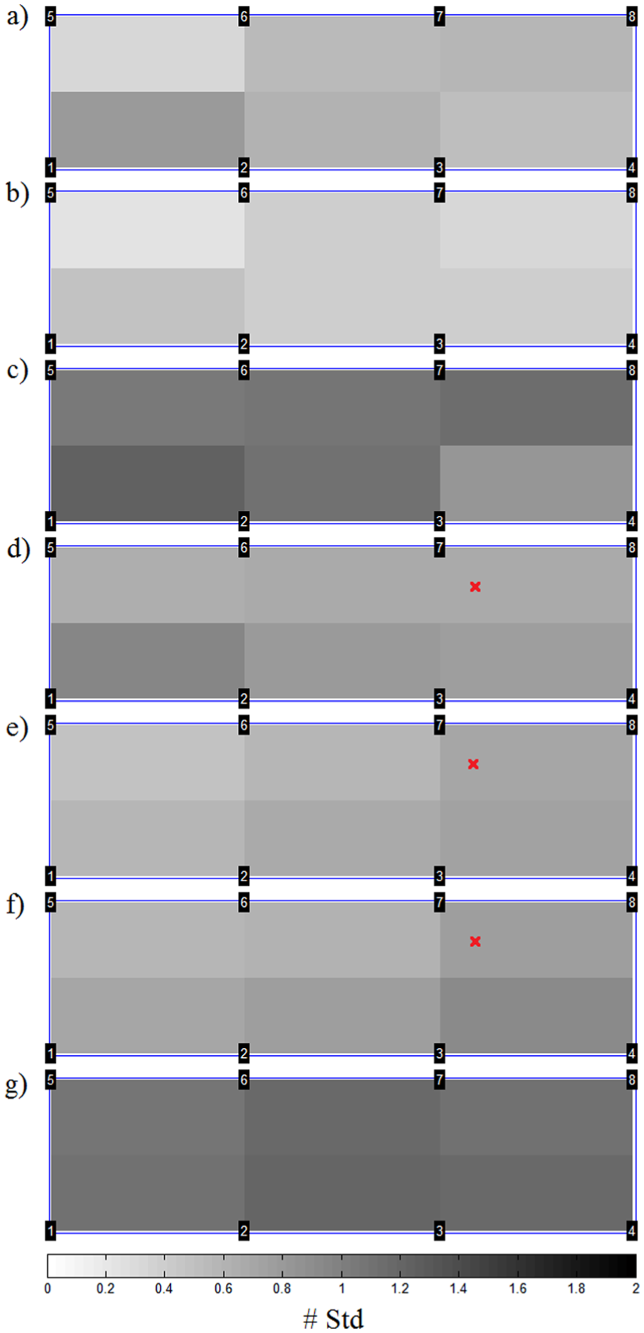
Results from the tomographic procedure at different times, using only phase data from the 50 kHz measurements. Sample numbers are (a) 400, (b) 600, (c) 700, (d) 727, (e) 735, (f) 773, and (g) 805. The red crosses denote the location of the damage. The gray scale signifies the deviation of the phase from the baseline data set, expressed in number of standard deviations of the baseline set. It is not possible to distinguish the healthy state from the damaged states using these images.

It is likely that the effects visible here would be less pronounced if, for example, transducers embedded into the concrete had been used instead of surface-mounted transducers that are more exposed to the environment. However, for the purposes of this study, it does not matter if the variations are introduced due to the concrete or due to the transducers, as both kinds of effects need to be accounted for in a realistic application.

Figure 6 shows the Mahalanobis distance between transducers 7 and 3 as a function of time (sample number). The Mahalanobis distance of each sample is calculated from the amplitude and phase values of all frequencies, and it is relative to a baseline consisting of the 300 preceding samples (corresponding to 1 week’s measurements) without any baseline lag. The first 300 measurements are used as the first baseline and are set to zero. For every new measurement, the baseline window is moved one sample ahead. Figure 6 shows some inherent deviation from the baseline at all times, with some variation. This is expected, since the EOV compensation is not perfect and there are some uncertainties in each measurement. However, some measurements clearly stand out in Figure 6, and these can be distinguished from the normal condition by the choice of a threshold value. These cases occur at sample numbers 727, 735, and 773, with a slightly wider peak at ∼805. The first three correspond to three clearly resolved damage events. The peak around 805 is not caused directly by a damage event, but is a false positive that is not successfully suppressed by the algorithm. There are two possible explanations. First, as can be seen from Figure 3, this was a particularly warm day with strong sunlight. The weather had changed suddenly from the previous 7 days, and the baseline did not contain enough data. Second, the temperature peak occurs on the first day after the last damage event. It is reasonable to assume that the influence of the EOVs on the measurements can be altered by the damage, for example by tension reliefs and exposure of inner materials, and that the Mahalanobis model has not yet “learned” this new behavior. If this is the case, then the variation is partly and indirectly caused by the damage, and it should rightfully be detected by the SHM system.

Figure 6.

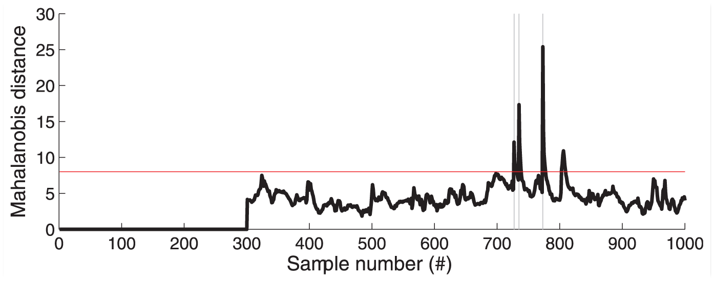
Mahalanobis distance for the measurements between transducers 7 and 3. A threshold line is set at a Mahalanobis distance of 8 (red horizontal line). The gray vertical lines indicate the times of the damage events.

Figure 7(a) to (g) shows the resulting images from the tomographic procedure at the same time stamps as in Figure 5, but in this case, the Mahalanobis distance is the damage indicator. Here, thresholds can easily be set to show no indications when there is no damage (Figure 7(a) to (c)). The time stamps corresponding to the damage events (Figure 7(d) to (f)) clearly indicate a deviation from normal behavior, and they also provide a rough indication as to between which transducers the damage occurred. Some indications are seen all over the slab, which is expected since the continuous diffuse wave fields consist of multiple scattered waves and boundary reflections. This phenomenon is expected to be somewhat less pronounced in larger structures where the transducers generally will be placed further from reflective boundaries.

Figure 7.

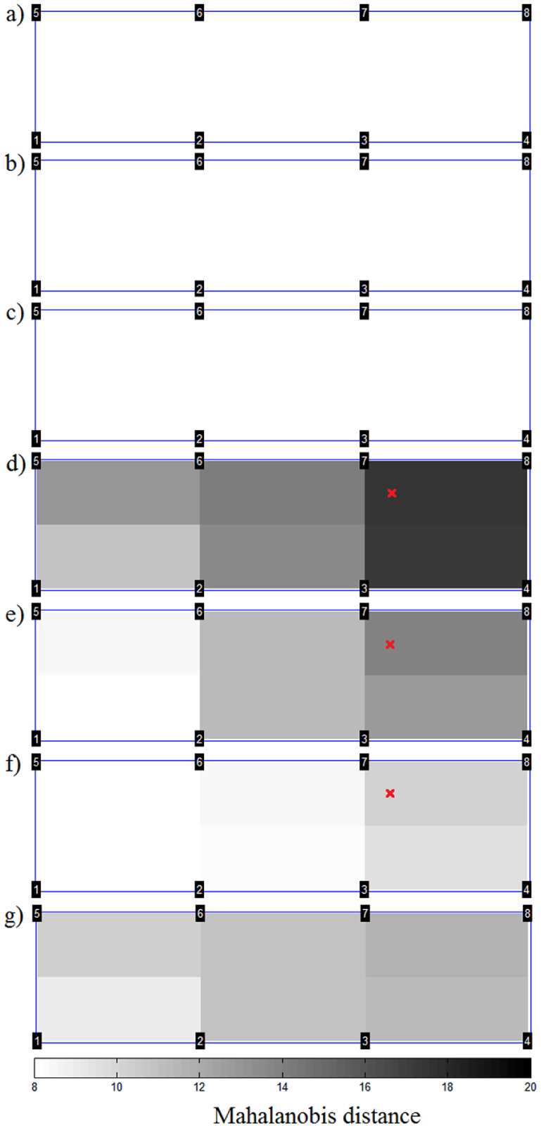
Results from the tomographic procedure after data normalization using the Mahalanobis distance. Sampling times (sample numbers) are (a) 400, (b) 600, (c) 700, (d) 727, (e) 735, (f) 773, and (g) 805. The red crosses denote the location of the damage. The damaged states can clearly be separated from the healthy state.

The images corresponding to the false positive at 805 (Figure 7(g)) show a slightly more homogeneous deviation over the slab, which is expected for a deviation caused by global EOVs. However, the grid coordinate containing the damaged area shows a slightly higher deviation than the rest of the slab. This possibly supports the reasoning described above—that this peak, at least in part, is caused indirectly by real damage.

The presented result did not use a lag in the moving window for the baseline. This led to sharp spikes for sudden events. After that, the damaged condition is included in the baseline and the behavior is classified as normal. This is suitable only for the detection of sudden events, which is the scope of this article. For slower degradation processes, a lag is needed between the baseline and each analyzed measurement. In a realistic scenario for a large structure that is exposed to the environment, one option is to use a lag of an entire year. The baseline period would correspond to the same season from the previous year. Alternatively, the method could be combined with the optimal baseline selection method mentioned in the Introduction section. Then, any slowly evolving damages should be detected as slow trends in the data. The possibility to detect slow deterioration in the material of a structure, with this method, will need to be verified in future studies.

Further improvements to the presented monitoring system could be to increase the number of frequencies used in the continuous-wave measurements. This would increase the dimensionality of each measurement. Then, principal component analysis could be used to remove some of the variations caused by the environmental conditions before applying the Mahalanobis distance tool, as described by Cross et al. ²⁹ Applying this technique to the data in this study did not improve the results. However, it could be of use if the dimensionality of the data is increased.

It should be stated that some parameters, such as selected frequencies, novelty threshold, and baseline lag, of the proposed SHM system have to be chosen from experience. Some will likely have to be tuned after the system has been in operation for a period of time, in order to find optimal settings.

The measurements in this study could likely be improved by the use of more sophisticated transducers, possibly embedded into the concrete, for example, those recently developed by Niederleithinger et al. ³⁰ The optimal placement of the transducers is not trivial and depends on the chosen frequencies and the geometry of the structure which is to be monitored.

Conclusion

Narrowband amplitude and phase measurements of diffuse wave fields, created by continuous-wave transmissions at different frequencies, were used to detect minor damage to a large concrete floor slab. A similar system has previously been shown to successfully detect and localize damage in mostly static environmental conditions. In this study, the system monitored the floor slab over 25 days, during which it was subjected to varying temperatures and sunlight exposure. These environmental conditions greatly influenced the measured data, and the resulting variations completely concealed the effect of the inflicted damage to the concrete. However, it was demonstrated that the variations caused by the environment could be largely suppressed using the Mahalanobis distance from a moving window baseline data set. Sudden damage events, which left centimeter-scale cracks in the concrete, could clearly be detected after this data normalization. Subsequently, a tomographic procedure, described in prior work by the authors, can be implemented to provide a rough localization of the damage.

Some of the environmentally caused variations remained after the data normalization. The most notable was a false-positive indication, on the same scale as the damage events, which was detected on a particularly warm and sunny day. This issue may be minimized in long-term measurements, where longer baselines can be used, which will include data from more environmental variations.

Nevertheless, the results from this study are encouraging for the use of diffuse ultrasonic wave fields in SHM applications for concrete structures, as the usability of such measurements are known to be very susceptible to environmental and operational variations.