Sage Journals: Discover world-class research

Abstract

This article presents the aerodynamic noise prediction of a NACA 0012 airfoil in stall region using Large Eddy Simulation and the acoustic analogy. While most numerical studies focus on noise for an airfoil at a low angle of attack, prediction of stalled noise has been made less sufficiently. In this study, the noise of a stalled airfoil is calculated using the spanwise correction where the total noise is estimated from the sound source of the simulated span section based on the coherence of turbulent flow structure. It is studied for the airfoil at the chord-based Reynolds number of 4.8 × 10⁵ and the Mach number of 0.2 with the angle of attack of 15.6° where the airfoil is expected to be under stall condition. An incompressible flow is resolved to simulate the sound source region, and Curle’s acoustic analogy is used to solve the sound propagation. The predicted spectrum of the sound pressure level observed at 1.2 m from the trailing edge of the airfoil is validated by comparing measurement data, and the results show that the simulation is able to capture the dominant frequency of the tonal peak. However, while the measured spectrum is more broadband, the predicted spectrum has the tonal character around the primary frequency. This difference can be considered to arise due to insufficient mesh resolution.

Keywords

Acoustics noise airfoil computational fluid dynamics LES Curle’s acoustic analogy

Introduction

Noise prediction is essential to control the sound emission in industrial applications, such as aircraft, wind turbines, road traffic, and so on. In order to identify the sound source or reduce the noise under those circumstances, the physical mechanism of sound generation needs to be understood deeply.

Airfoil noise has been of great interest to researchers for many years. It is considered that turbulent eddies are convected along the chord and these vortices are scattered from the trailing edge. The acoustic wave propagates to the far field, and it is heard as either broadband or tonal noise. Paterson et al.¹ found that noise caused by airfoil-shedding vortices are discrete rather than broadband, and the tonal frequency is related to the Strouhal number normalized with the boundary layer thickness at the trailing edge. Arbey et al.² experimentally showed the process of the so-called aeroacoustic feedback loop that the acoustic wave generated from the trailing edge propagate to upstream, which in turn enhances the oscillation of the boundary layer there and causes the discrete noise. Brooks et al.³ identified five mechanisms associated with airfoil self-noise generation and derived the semi-empirical equations. These five mechanisms are the laminar and turbulent boundary layer noise, separation-stall noise, tailing-edge bluntness noise, and tip vortex noise.

Several studies to predict the acoustic field around an airfoil using computational fluid dynamics (CFD) simulations have been reported. Desquesnes et al.⁴ studied the tonal noise phenomenon by conducting two-dimensional direct numerical simulation of the flow around a NACA 0012 airfoil. They verified that a separation bubble close to the trailing edge on the pressure side amplifies the tonal noise and that the phase difference between the hydrodynamic fluctuations on the suction and pressure sides has an impact on the amplitude of the acoustic waves. Boudet et al.⁵ carried out Reynolds-averaged Navier–Stokes (RANS) simulations and Large Eddy Simulation (LES) on a rod-airfoil configuration, and they compared both results to experimental data. The RANS approach only predicted the tonal noise, whereas the LES resulted in a good sound computation for both broadband and discrete sound. Wang et al.⁶ investigated turbulent boundary-layer flow past a trailing edge of a flat strut using LES, aiming at numerically predicting the broadband noise caused from boundary layers on a sharp edge. They found that a wider computational domain is needed for predicting noise at low frequencies. Manoha et al.⁷ conducted compressible three-dimensional LES to compute the far field noise for a NACA 0012 airfoil. The local flow is solved by LES for the near-field region, and noise propagation is simulated using the linearized Euler equations and the Kirchhoff integral for the midfield and far-field regions. They concluded that a key point is how to couple the boundaries between these fields accurately.

There are many applications of rotating machines such as a propeller fan and a wind turbine blade where massive vortex shedding is involved due to large flow separation when they are not operated in an optimal condition. Therefore, the importance of understanding stalled flow noise, which can be a high contribution of sound sources, has been emphasized. For instance, Fink and Bailey⁸ stated in their airframe noise study that the noise at stall is increased by more than 10 dB relative to the noise emitted at low angles of attack. However, few studies have been presented for acoustic prediction of the airfoil in stall condition where the flow features and the corresponding acoustic radiation are quite different from those of the airfoil at small angles of attack. One related example is a work from Suzuki et al.⁹ where the sound source is identified for a flow field around a NACA 0012 airfoil in both the light and deep stall conditions. There is another study by Christophe et al.¹⁰ and Moreau et al.¹¹, who performed acoustic measurements for an airfoil at a high angle of attack to model the acoustic noise using Amiet’s theory and Curle’s analogy. The wake vortex around airfoil in the stall region can be attributed to the main noise source, which makes noise prediction challenging. These vortices have large structures relative to the chord length, and thus the CFD analysis around the airfoil in stall needs a large domain size in the spanwise direction to capture the full vortex structures. Due to high computational cost, it also may not be feasible to extend the domain size while keeping the sufficient mesh resolution to capture small fluctuations of pressure.

This study presents a numerical approach for the self-noise prediction of a stalled airfoil using LES and the acoustic analogy. The prediction is performed by employing the spanwise correction method proposed by Seo and Moon¹² to correct the sound pressure considering the degree of correlation of the turbulence flow structure along the span, so that less spanwise extent of the domain needs to be simulated. The spanwise correction has been applied in many works investigating noise emission for long-span bodies involved with vortex shedding such as a cylinder, but not an airfoil. While most of the previous studies for airfoil noise prediction simply assume the homogeneous turbulence of the sound source, the correction is necessary for noise prediction of a stalled airfoil where the characteristic length of the vortex shedding is relatively large compared to that of an airfoil at a low angle of attack. The numerical model uses the hybrid method which decouples the sound source generated due to aerodynamics with the acoustic wave propagation. The flow of the near-field region around an airfoil is solved using LES, and Curle’s acoustic analogy is used to calculate the sound propagation to the far-field region.

The predicted results are validated by comparing data measured by Brooks et al.³ A model of a NACA 0012 airfoil section is investigated which has a chord length of 10.16 cm and 15.6° angle of attack. The freestream velocity is 71.3 m/s, which leads to the condition that the Reynolds number based on the chord length is 4.8 × 10⁵ and the Mach number is 0.2. The simulated span length is 4.5 cm that accounts for 1/10 of the experimental model. The sound received at 1.2 m from the trailing edge of airfoil in the direction perpendicular to the freestream wind in the midspan plane is presented for validation.

Computational method

Acoustic prediction

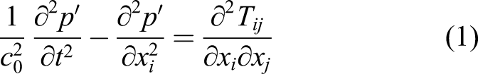
CFD simulations are performed to calculate the aerodynamic sound source, and then the propagation of sound to the far field is obtained using Curle’s acoustic analogy. The theory of the acoustic analogy is explained in this section. Lighthill¹³ first proposed a generalized equation of the wave propagation for an arbitrary acoustic source region surrounded by a quiescent fluid. He derived the equation for the acoustic perturbations from mass and momentum conservation, assuming that there are no external forces acting on a fluid. Here, the fluctuation of pressure and density are defined as p′ = p − p₀ and ρ′ = ρ − ρ₀, where p₀ and ρ₀ are constants in a reference fluid at rest far from the sound source. The derived equation of the so-called Lighthill’s analogy is written as

\frac{1}{c_{0}^{2}} \frac{\partial^{2} p^{'}}{\partial t^{2}} - \frac{\partial^{2} p^{'}}{\partial x_{i}^{2}} = \frac{\partial^{2} T_{i j}}{\partial x_{i} \partial x_{j}}

(1)

where

T_{i j} = ρ u_{i} u_{j} + P_{i j} - c_{0}^{2} (ρ - ρ_{0}) δ_{i j}

is the Lighthill stress tensor, u_i is the fluid velocity in the i direction, P_ij is the compressive stress tensor that includes the surface pressure and the viscous stress, c₀ is the speed of sound in a reference fluid, and δ_ij is the Kronecker delta.

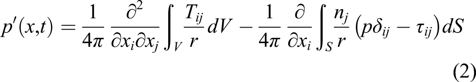
Curle¹⁴ derived the solution of the Lighthill’s equation for flows in the presence of static solid boundaries using the free space Green’s function. The solution, called the Curle’s analogy, can be written as

p^{'} (x, t) = \frac{1}{4 π} \frac{\partial^{2}}{\partial x_{i} \partial x_{j}} \int_{V} \frac{T_{i j}}{r} d V - \frac{1}{4 π} \frac{\partial}{\partial x_{i}} \int_{S} \frac{n_{j}}{r} (p δ_{i j} - τ_{i j}) d S

(2)

where r is the distance between the sound source and the sound-receiving position, n_j is the unit vector normal to the surface, and τ_ij is ρu_iu_j. Equation (2) represents the sound pressure with integrals of the total volume external to the surface V and the surface of the boundaries S. The integrals are to be evaluated at the retarded time τ = t − r/c₀, where t is time at the receiver. The spatial derivative can be converted as

\frac{\partial}{\partial x_{i}} = \frac{\partial}{\partial τ} \frac{\partial τ}{\partial x_{i}} = - \frac{1}{c_{0}} \frac{\partial r}{\partial x_{i}} \frac{\partial}{\partial τ} = - \frac{l_{i}}{c_{0}} \frac{\partial}{\partial τ}

(3)

where l_i is the unit vector pointing from the source location to the receiver.

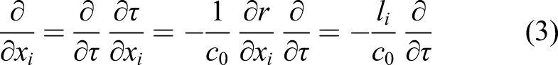
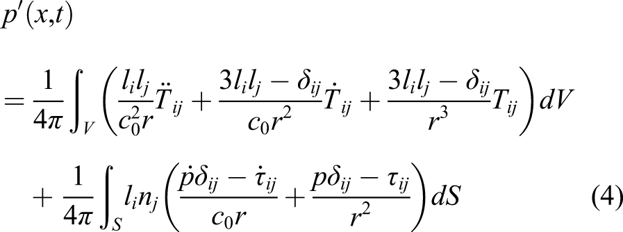
Larsson et al.¹⁵ rewrites equation (2) based on the formations by Brentner et al.¹⁶ The expression in equation (2) is modified to a form where the spatial derivative is converted to a temporal one using equation (3) and the derivatives are taken inside the integral. Then, p′( x , t) is expressed as

\begin{array}{l} p^{'} (x, t) \\ = \frac{1}{4 π} \int_{V} (\frac{l_{i} l_{j}}{c_{0}^{2} r} {\ddot{T}}_{i j} + \frac{3 l_{i} l_{j} - δ_{i j}}{c_{0} r^{2}} {\dot{T}}_{i j} + \frac{3 l_{i} l_{j} - δ_{i j}}{r^{3}} T_{i j}) d V \\ + \frac{1}{4 π} \int_{S} l_{i} n_{j} (\frac{\dot{p} δ_{i j} - {\dot{τ}}_{i j}}{c_{0} r} + \frac{p δ_{i j} - τ_{i j}}{r^{2}}) d S \end{array}

(4)

where dots such as

\dot{p}

indicate a derivative with respect to time. In this study, the term for the volume integral, which represents quadrupole source terms, is neglected and only the second term, which corresponds to the dipole sound source generated by the force on the surface, is considered. This is because the contribution of the quadrupole sources to the total sound is generally expected to be much smaller than that of the dipole source for flows in a low Mach number regime.¹⁷ Also, it can be assumed in almost all cases that the surface source term is determined by the surface pressure and the viscous stresses on the surfaces τ_ij are negligible.¹⁸ Thus, the equation used in our calculation is reduced to the following form.

p^{'} (x, t) = \frac{1}{4 π} \int_{S} l_{i} n_{j} (\frac{\dot{p} δ_{i j}}{c_{0} r} + \frac{p δ_{i j}}{r^{2}}) d S

(5)

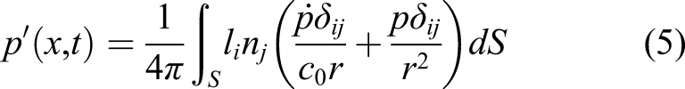
It is noted that an incompressible flow simulation is performed in this study, although incompressibility assumption is not physically compatible with acoustic phenomena. When the interaction between turbulence and body surface occurs in a region that is compact enough, incompressible flow solutions can be adequate for approximating acoustic source terms.^10,19 There are many noise problems in the field of aeroacoustics at low Mach numbers where the acoustic sources are compact, and in such cases, the fluid may be treated as an incompressible flow.²⁰ For the present case, the sound source is regarded as compact in the frequency range of interest. The chord length is comparable to the wavelength corresponding to the frequency of around 3400 Hz, and the dominant noise lies in the frequency range of one order lower than that.

Aerodynamic calculation

The flow characteristics for sound prediction are obtained by the CFD computation. Incompressible Navier–Stokes equations are solved using LES based on the finite volume method. As a subgrid-scale (SGS) model, one equation eddy viscosity model²¹ is used where the SGS eddy viscosity is expressed by using the SGS kinetic energy and the grid width, and the transport equation for the SGS kinetic energy is solved at every time step.

The second-order upwind total variation diminishing scheme²² is applied for discretization of the convective terms. The diffusive terms are discretized by the central difference scheme. The time integration is represented by the second-order upwind Euler scheme. The pressure–velocity coupling is solved by the PIMPLE algorithm, which is developed for transient problems and is a combination of the PISO and SIMPLE algorithm.

Figure 1 shows the computational domain and the boundary conditions. A NACA 0012 airfoil inclined by an angle of attack is located at the origin. The dimensions in x direction from the airfoil to inlet and outlet are 20c and 54c, respectively, where c is the chord length. The domain height in the y direction is 37c. The simulated airfoil has a span length of L_s = 0.4c = 4.46 cm. This size is equal to 10% of the span length of the experimental model, which is L = 45.72 cm. The constant incoming velocity is specified as U₀ = 71.3 m/s at the inlet boundary, and the pressure is set to zero at the outlet boundary. The slip condition is used at the boundaries in the y direction. On the airfoil surface, the velocity is set to zero with no wall function for the boundary layer approximation applied. Both symmetry and periodic conditions are tested to examine the influence of the boundary condition in the spanwise direction. Additional test cases are run with a larger domain size L_s = 1.3c to validate the applicability of the spanwise correction method for the present domain.

Figure 1.

Computational domain and boundary conditions.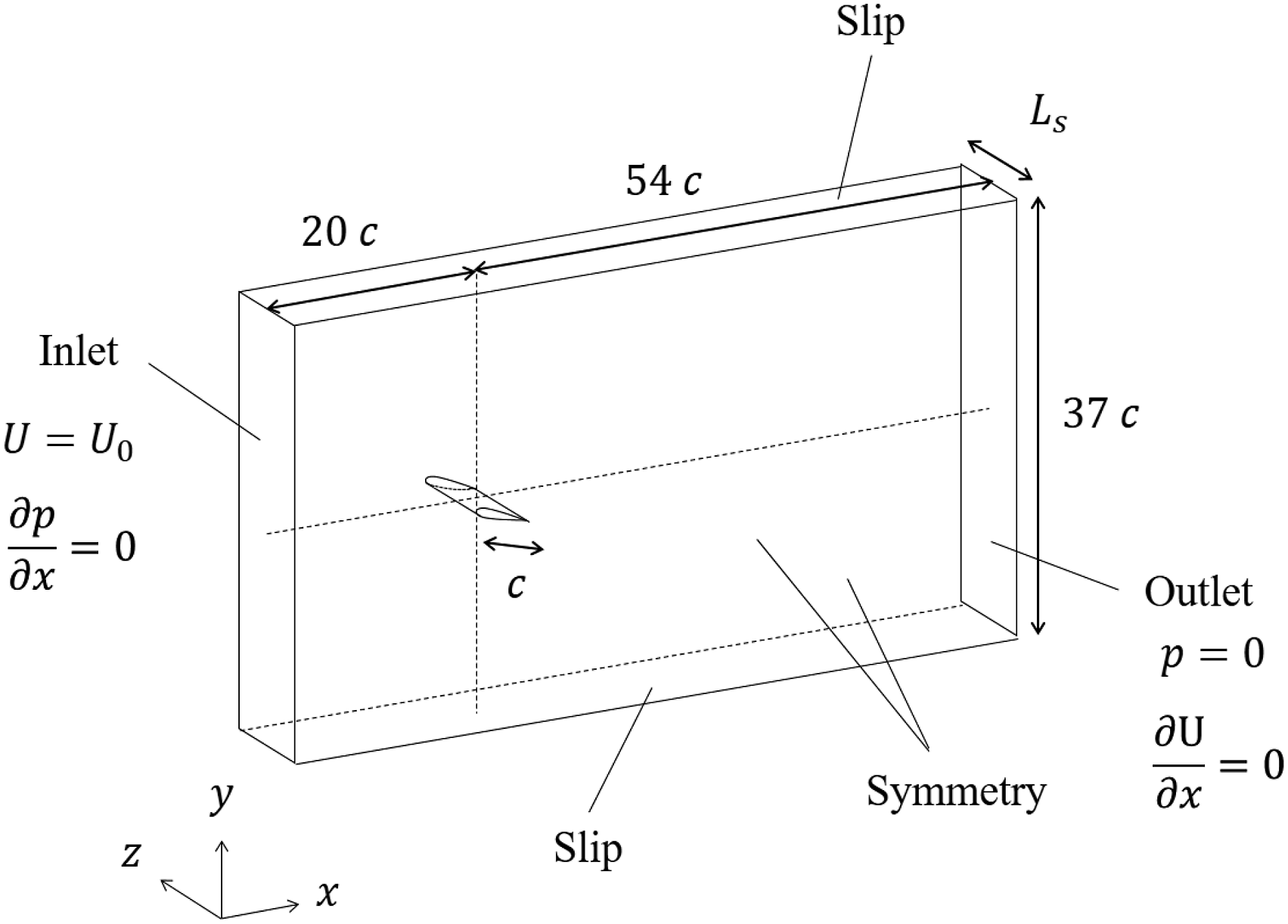

Spanwise correction

In order to predict the sound pressure p′ emitted from the entire airfoil surface of the span length L, it is necessary to extrapolate the sound source outside the computational domain from the sound source simulated with the span section L_s. Here, the sound pressure generated from the span sections L and L_s are denoted as $p_{all}^{'}$ and $p_{s}^{'}$ , respectively. If the sound source occurs along the span independently in the statistical sense, the sound power can be approximated to be proportional to the span length, that is, $p_{all}^{' 2} / p_{s}^{' 2} \propto L / L_{s}$ . Wolf et al.²³ applied this approximation in their study where the sound source separated by the simulated spanwise width radiates independently from neighboring sources. Moreau et al.²⁴ explains that the sound intensity I = p′²/ρc₀ can be assumed to be proportional to the squared span length, that is, $p_{a l l}^{' 2} / p_{s}^{' 2} \propto L^{2} / L_{s}^{2}$ , if the pressure fluctuates in phase along the whole span, or in other words, the sound source can be considered as two-dimensional.

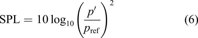
This study employs the spanwise correction proposed by Seo and Moon,¹² and the theory for the correction is briefly explained below. They proposed a noise prediction methodology for long-span bodies by revisiting a simple correction suggested by Kato et al.²⁵ and Pérot et al.²⁶ The sound pressure level (SPL) is defined as

SPL = 10 \log_{10} {(\frac{p^{'}}{p_{ref}})}^{2}

(6)

where the reference pressure p_ref is the threshold of human hearing, 2 × 10⁻⁵ Pa. Let us denote the SPL generated from sections L and L_s as SPL_all and SPL_s. So,

{SPL}_{all} = {SPL}_{s} + {SPL}_{cor}

(7)

where SPL_cor is the SPL needed for correction. SPL_cor is defined below as a function of frequency f

\begin{array}{l} {SPL}_{cor} (f) \equiv \\ \begin{array}{l} {\begin{matrix} 20 l o g (\frac{L}{L_{s}}) & (\frac{L}{\sqrt{π} L_{s}} \leq \frac{L_{c}}{L_{s}}) \\ 10 l o g (\frac{L_{c}}{L_{s}}) + 10 l o g (\frac{\sqrt{π} L}{L_{s}}) & (\frac{1}{\sqrt{π}} < \frac{L_{c}}{L_{s}} < \frac{L}{\sqrt{π} L_{s}}) \\ 10 l o g (\frac{L}{L_{s}}) & (\frac{L_{c}}{L_{s}} \leq \frac{1}{\sqrt{π}}) \end{matrix} \end{array} \end{array}

(8)

where L_c is the spanwise coherence length determined from the spanwise coherence function, which is also a function of f. The correction is made based on the degree of the spanwise coherence of the turbulence structures. The first expression in equation (8) is used if the pressure fluctuation occurs in phase, and the last expressioin is used if the pressure fluctuates inhomogeneously. The middle expression is applied when the phase difference falls into the range between these two extreme cases.

The coherence length L_c is calculated as follows. Consider the case where the blade of span length L_s is divided into N subsections in the spanwise direction as shown in Figure 2. Let us denote the power spectral density of sound pressure radiated from a subsection N_i as ${\hat{p}}_{i}^{'}$ . The sound pressure radiated from each subsection is lagged by a phase difference which can be characterized by the coherence function

γ_{i, j}^{'} (f, Δ z_{i, j}) = \frac{\bar{Re ({\hat{p}}_{i}^{'} {\hat{p}}_{j}^{' *})}}{\sqrt{{| {\hat{p}}_{i}^{'} |}^{2}} \sqrt{{| {\hat{p}}_{j}^{'} |}^{2}}}

(9)

Figure 2.

Schematic of the subdivided blade for spanwise correction.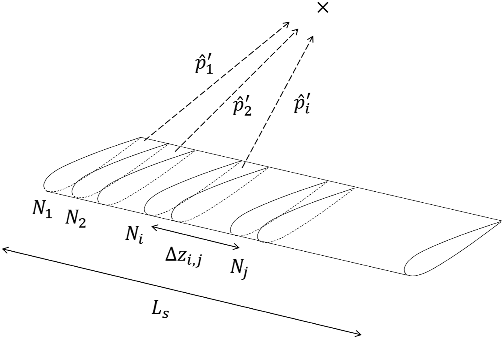

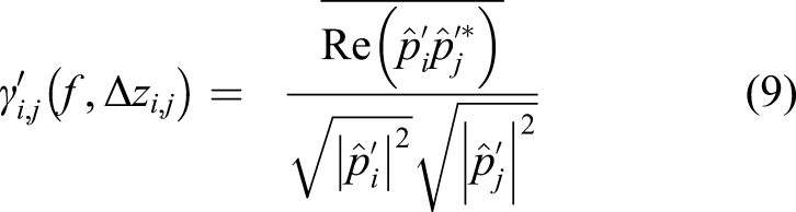
This is a function of the distance between two subsections, Δz_i,j. Since the phase lagging in the spanwise direction tends to follow a Gaussian distribution,²⁷ the acoustic spanwise coherence function γ′(Δz) can also be expressed as

γ^{'} (f, Δ z) = \exp (- \frac{Δ z^{2}}{L_{c}^{2}})

(10)

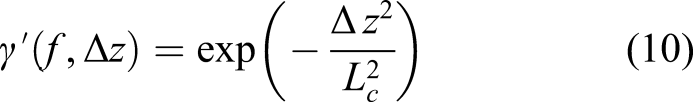
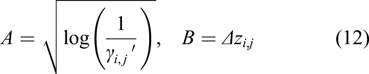
The value of L_c in equation (10) is determined so as to satisfy to best fit the Gaussian distribution function γ′ for a set of Δz_i,j and $γ_{i, j}^{'} (Δ z_{i, j})$ obtained in equation (9).

Study cases

This article includes five run cases as listed in Table 1. A reference test case is presented as CASE A. It is necessary to make sure that the simulated span extent L_s is sufficient to apply the spanwise correction for predicting the total noise. Thus, two cases are run with the same domain size L_s = 0.4c (CASE B) and a three times larger size L_s = 1.3c (CASE D). While the symmetry boundary condition is applied in the reference case, the periodic condition is tested as well. The cases using the periodic condition with the domain size L_s = 0.4c and L_s = 1.3c correspond to CASE C and CASE E, respectively.

Table 1.

Five test cases studied in this paper.

CASE	L _s	Number of mesh points	BC	Duration of simulated time steps
A	0.4c	49 million	Symmetry	0.0535 s
B	0.4c	16 million	Symmetry	0.2095 s
C	0.4c	16 million	Periodic	0.1654 s
D	1.3c	47 million	Symmetry	0.0626 s
E	1.3c	47 million	Periodic	0.0844 s

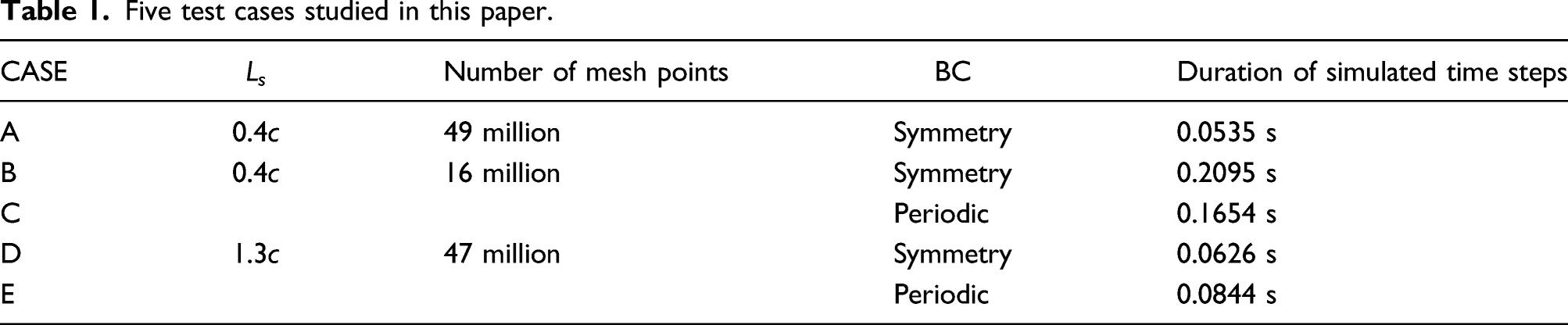
The flow domain is discretized using structured grids. The mesh used in CASE A consists of about 49 million cells. The geometry of an airfoil configuration is meshed with approximately 1134 and 257 points along the chord and span, respectively. Figure 3 shows the zoomed view of the mesh around the airfoil. The grid spacing in the direction normal to the wall y⁺ is below unity for the mesh of CASE A over the entire surface of the airfoil. In order to complete simulations in reasonable computational time, the coarse mesh is used for CASE B to CASE E which has double spacing in the region ranging from −1.2c to 5.9c and from −0.7c to 0.8c in x and y directions, respectively.

Figure 3.

Zoomed view of the discretized mesh around airfoil.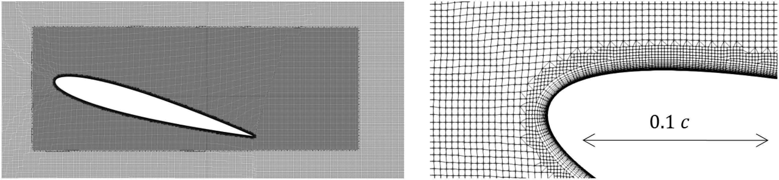

The RANS simulation with the k − ω SST turbulence model²⁸ is conducted to provide initial flow fields. The data from LES are extracted after the flow becomes converged. Table 1 also lists the duration of simulated time steps used for acoustic calculations.

The parallel computation is run using 128 processors on the Tetralith cluster provided by the NSC (National Supercomputer Centre) at Linköping University. The computational domain is split into 128 subdomains, and each subdomain is assigned to one of the processors.

The airfoil model under the experimental setup causes downwash deflection of the incident flow. In the measurement, side plates are flush mounted on the jet nozzle lip and the airfoil is held between these plates. The proximity of the airfoil to the jet nozzle and the limited jet width can cause the airfoil pressure loading and flow characteristics to deviate significantly from those measured in free air,²⁹ and this can effectively reduce the angle of attack.

Considering the downwash effect, the result simulated with 15.6° angle of attack is validated against the data measured with 19.8° angle of attack. Brooks et al.³ claim that the effective angles of attack is 12.3° for the geometrical angle of 19.8° according to the lifting surface theory.³⁰ However, it can be considered that the lifting surface theory is valid only for attached flows and thus is not well suitable to apply to the airfoil in the post-stall regime. Therefore, the effective angles of attack were examined using the RANS simulation.³¹ In the simulation, the full wind tunnel setup was reproduced, including the jet nozzle, the fully scaled airfoil model, and the side plates. The flow curvature caused by the downwash effect was reproduced, as shown in Figure 4 illustrating an example when the angle of attack is 19.8°. Considering the angle of the flow direction observed in the wake behind the airfoil, it was concluded that 19.8° angle of attack should be corrected to 16.6°, instead of 12.3°.

Figure 4.

Velocity field around an airfoil of 19.8° angle of attack obtained from RANS simulation considering the wind tunnel configuration.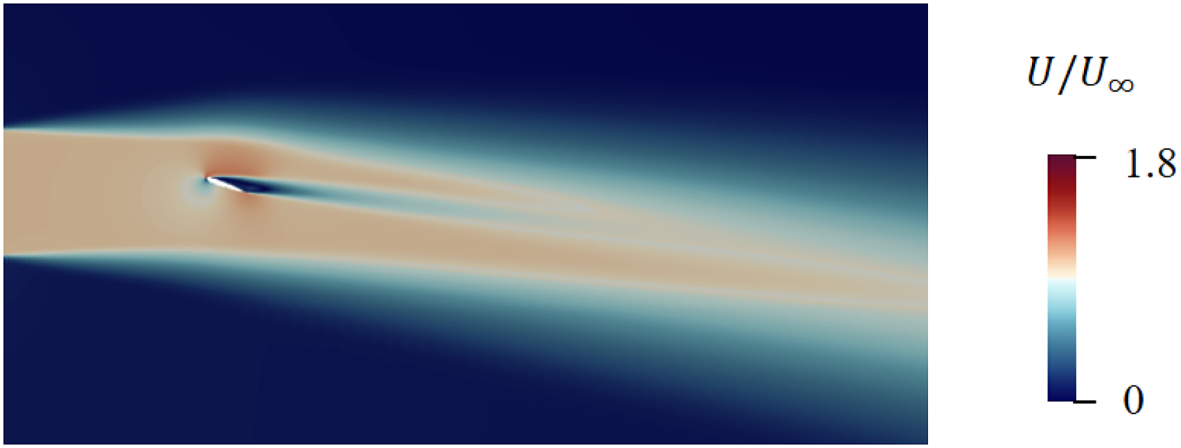

Results and discussion

Flow characteristics

Figure 5 shows the instantaneous velocity field around the airfoil and the isocontour of the vorticity. Each picture depicts the magnitude of velocity U normalized with U₀ and the magnitude of the vorticity which is calculated by ω = ∇ × U. It can be observed that the flow is separated from the leading edge and sheds large-scaled vortices from the whole surface on the suction side. Small-scaled vortices can also be seen covering the entire upper surface of airfoil.

Figure 5.

Instantaneous velocity field (left) and isocontour of the magnitude of vorticity |ω| =5000 s⁻¹ (right).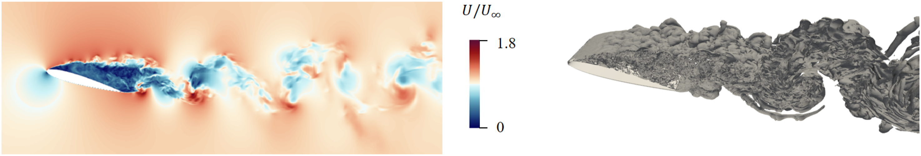

The velocity is sampled at 0.2c downstream from the trailing edge to check the vortex-shedding frequency, and it shows clear periodicity at 497 Hz. It is also sampled at 0.3c downstream from the leading edge where vortices caused by the Kelvin–Helmholtz instability in the shear layer can be observed. The spectrum of the velocity, which is not presented, indicates that there is a highest but moderate peak in the range between 2500 and 3000 Hz.

Figure 6 shows the time derivative of the pressure on the airfoil surface $\dot{p}$ , which is a variable with a major contribution to the sound pressure p′. The values depicted are scaled with the range of $\dot{p} = \pm 1.5 \times 10^{6} Pa / s$ . It is interesting to note that $\dot{p}$ behaves differently depending on the chord location. The pressure fluctuates with small-scaled structures at the rear of the airfoil, while the wavelike change occurs in the front half of the airfoil, being highly constant along the span.

Figure 6.

Time derivative of surface pressure 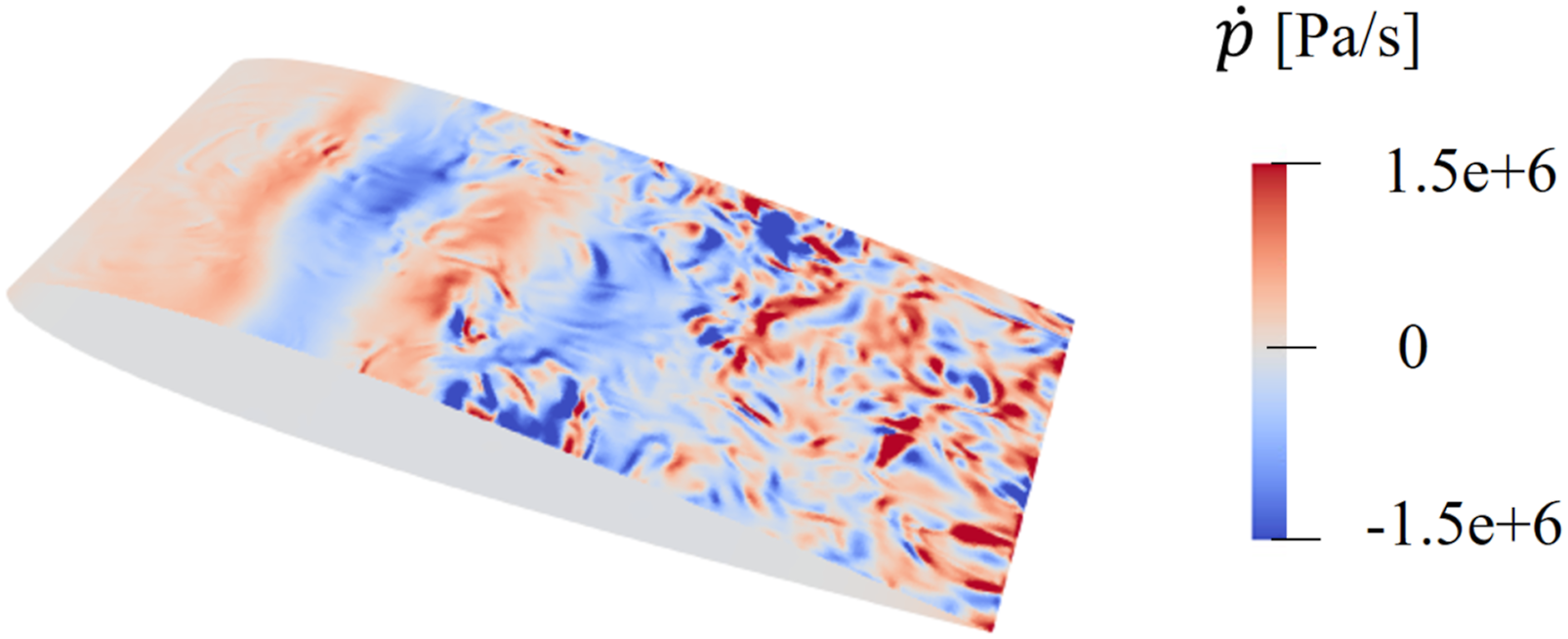$\dot{p}$ .

Figure 7 shows the power spectral density of the pressure fluctuation at chordwise locations of 0, 0.2c, 0.5c, and 0.95c on the suction and 0.95c on the pressure sides. The spectral density in dB per Hz is calculated with the reference of p_ref. The surface pressure is probed at 12 equally spanwise-distributed points. Time histories of the probed pressure are subdivided into 8 sections to take the average spectrum at each sampling point, and then the mean spectra is calculated from the averaged 12 spectra of each chord location.

Figure 7.

Power spectral density of the surface pressure fluctuation at chordwise locations of 0, 0.2c, 0.5c, and 0.95c on the suction and 0.95c on the pressure sides with reference to 2 × 10⁻⁵ Pa.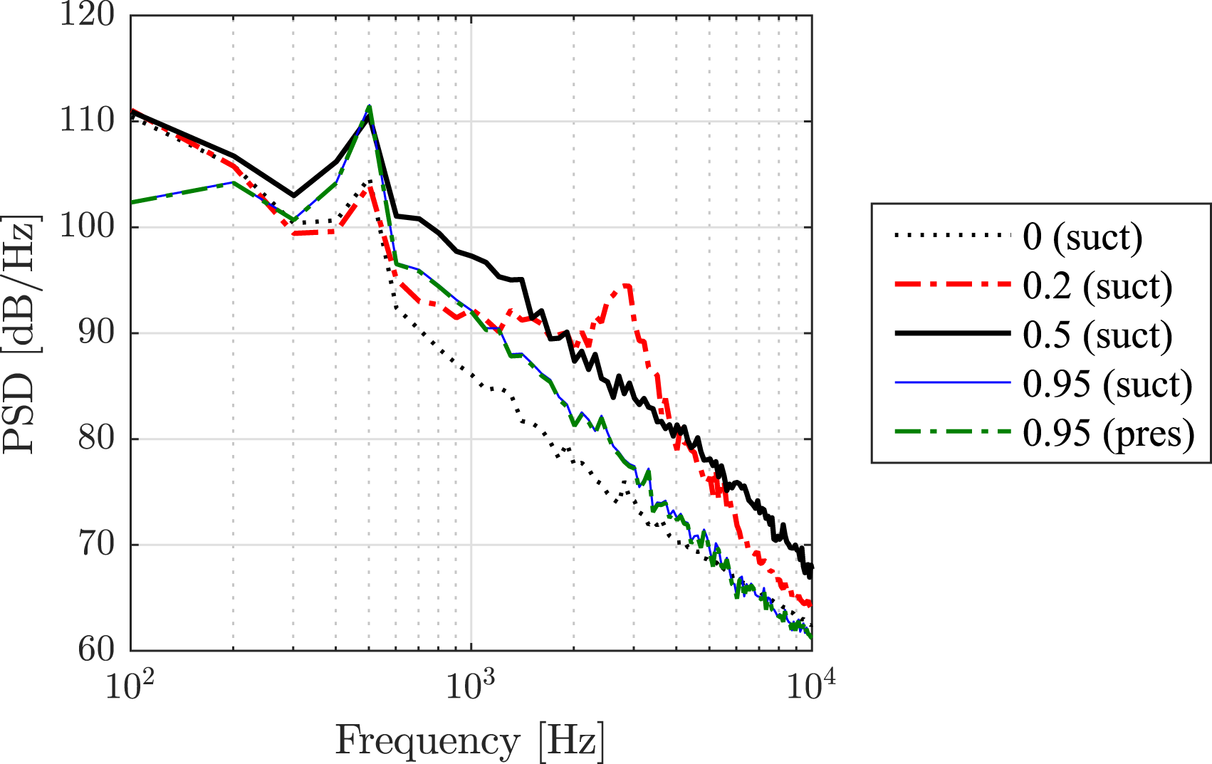

The dominant peaks are clearly seen at 502 Hz at all chordwise locations, and it is considered that these peaks are caused due to large vortices shed in the wake. All spectra decay at high frequencies. There is a second peak at 2913 Hz for the location of 0.2c. The wave pattern of the surface pressure derivative $\dot{p}$ in the front half of airfoil is observed in Figure 6, and it can be considered that this peak at the location 0.2c arises due to the vortices formed in the shear layer close to the leading edge. The spectra also indicate that the surface pressure at the location of 0.5c is highest at almost all frequencies except at around 2913 Hz. The pressure at 0.95c has close amplitude on both airfoil sides.

Figure 8 shows the pressure coefficient C_p, which is defined as $p / 2 ρ U_{0}^{2}$ , plotted with the measurement data by Michos et al.³² The x axis represents the chordwise distance, x_c. The solid and dotted lines represent the time-averaged and instantaneous values of the simulation. The Reynolds number of measurement is not exactly the same but is closest among available data that can be referred. Since there is no angle of attack data which coincide with the simulated one, both the data for 14° and 20° angles are presented.

Figure 8.

Pressure coefficient C_p of time-averaged (solid line) and instantaneous (dotted line) values from LES (AOA = 15.6°, Re = 4.8 × 10⁵) compared with measurement by Michos et al.³² (AOA = 14° and 20°, Re = 7.6 × 10⁵) against the chordwise coordinates x_c.

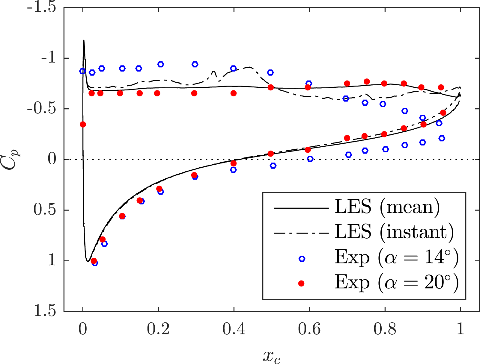
A uniform distribution on the upper surface implies the flow separation, and this behavior can be observed from both the simulation and the measurement. Michos et al.³² stated that the angle of attack at 14° is the point where the airfoil starts to become completely stalled. The predicted C_p curve agrees better with the values measured at 20° than those at 14°, and it seems that the simulation represents the airfoil which is deeply stalled.

Acoustic calculation

Procedure for spanwise correction

The simulated flow properties related to the sound source is statistically extrapolated for the region outside of the computational domain to predict the noise generated from the entire span section. The procedure for calculation of SPL_cor is presented in this section.

The span of airfoil is divided into 5 subsections, N₁, …, N₅ (see Figure 2). Both ends of length L_s/12 are not used to avoid including the boundary effect. Time histories of the sound pressure radiated from each subsection are split into 8 blocks with an overlap ratio of 50% for intervals of 0.0134 s, which corresponds to 13,372 time samples. This results in the resolution of frequency of 75 Hz. The Hanning window is applied, and then FFT is performed for each block. The auto power spectra for ${\hat{p}}_{1}^{'}$ , …, ${\hat{p}}_{5}^{'}$ and the cross spectra between ${\hat{p}}_{i}^{'}$ and ${\hat{p}}_{j}^{'}$ for all combinations of i and j (i, j = 1, …, 5 and i ≠ j) are calculated, and they are averaged from all the 8 spectra. Then, the coherence functions $γ_{i, j}^{'}, (Δ z_{i, j})$ are obtained as a function of frequency and the distance Δz_i, j.

L_s(f) is the parameter of the distribution function γ′ and is determined by applying the least-square fitting to the data points Δ z_i, j and $γ_{i, j}^{'}$ at each frequency. We have a data set of Δz_i,j and $γ_{i, j}^{'}$ , and the value of L_c is estimated using a linear equation

B = L_{c} \cdot A

(11)

which is the rearrangement of equation (10) where

A = \sqrt{\log (\frac{1}{γ_{i, j}^{'}})}, B = Δ z_{i, j}

(12)

Figure 9 shows the coherence functions at three selected frequencies, 299 Hz, 524 Hz, and 748 Hz, when they are viewed as a function of the spanwise distance. The x axis represents the distance Δz normalized with L. The simulated span extent L_s corresponds to Δz/L = 0.1. The obtained four data points Δz_i,j and

γ_{i, j}^{'},

for each frequency are depicted with markers, and the curves of the Gaussian distribution functions γ′ obtained by fitting are plotted as well.

Figure 9.

Coherence function γ′ at three selected frequencies, 299 Hz, 524 Hz, and 748 Hz plotted against normalized spanwise distance Δz/L.

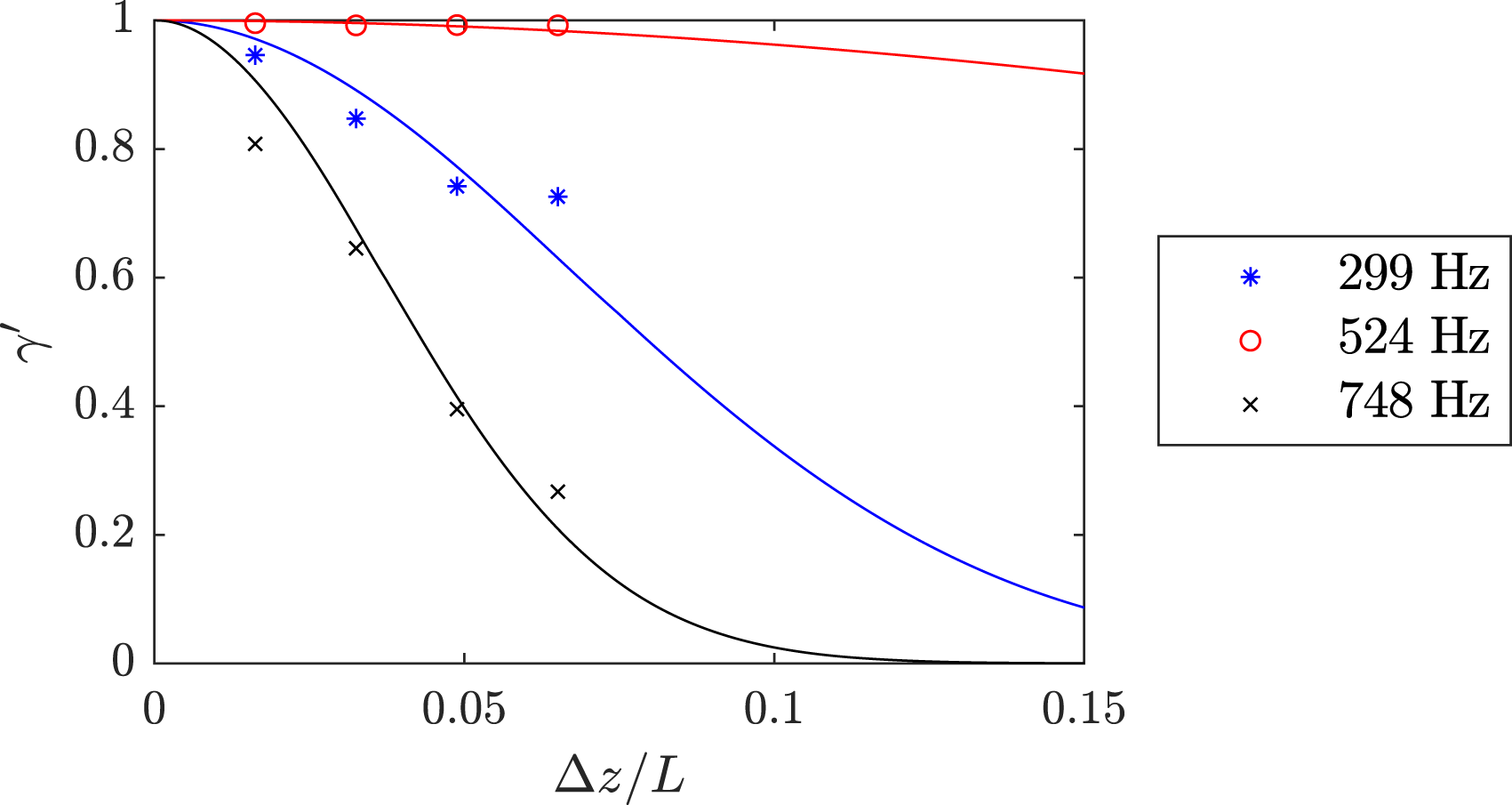
The curves in Figure 9 show the distance decay of the coherence. The coherence function at 524 Hz, which is close to the vortex-shedding frequency, remains high and is larger than 0.9 even at Δ z/L = 0.1. When the flow is attached at low angles of attack, vortices around the airfoil surface have small-scaled structure, and thus the coherence drops with short distance. If the airfoil is in stall and generated vortices are relatively large, the coherence is high even at long distance as seen in this case. This needs to be considered properly especially when the computational domain size is limited. On the contrary, the curve at 748 Hz indicates a rapid decrease within the distance of the simulated span length.

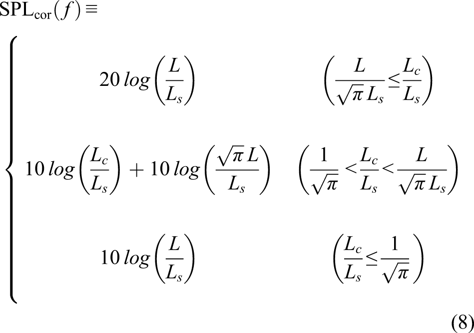
SPL_cor is obtained based on equation (8) using the coherence length L_c for each frequency. Figure 10 shows L_c normalized with L_s and SPL_cor represented by the black (thin) and red (bold) lines, respectively. According to the correction method, SPL_cor is at maximum, 20 dB, if L_c/L_s is larger than 5.8, while SPL_cor is at minimum, 10 dB, if L_c/L_s is smaller than 0.6. The results show that the coherence length is large and SPL_cor becomes almost maximum at around the vortex-shedding frequency. They sharply decrease at high frequencies, and SPL_cor becomes close to the minimum value at frequencies larger than 1000 Hz.

Figure 10.

Spanwise coherence length L_c normalized with L_s and the sound pressure level for correction SPL_cor.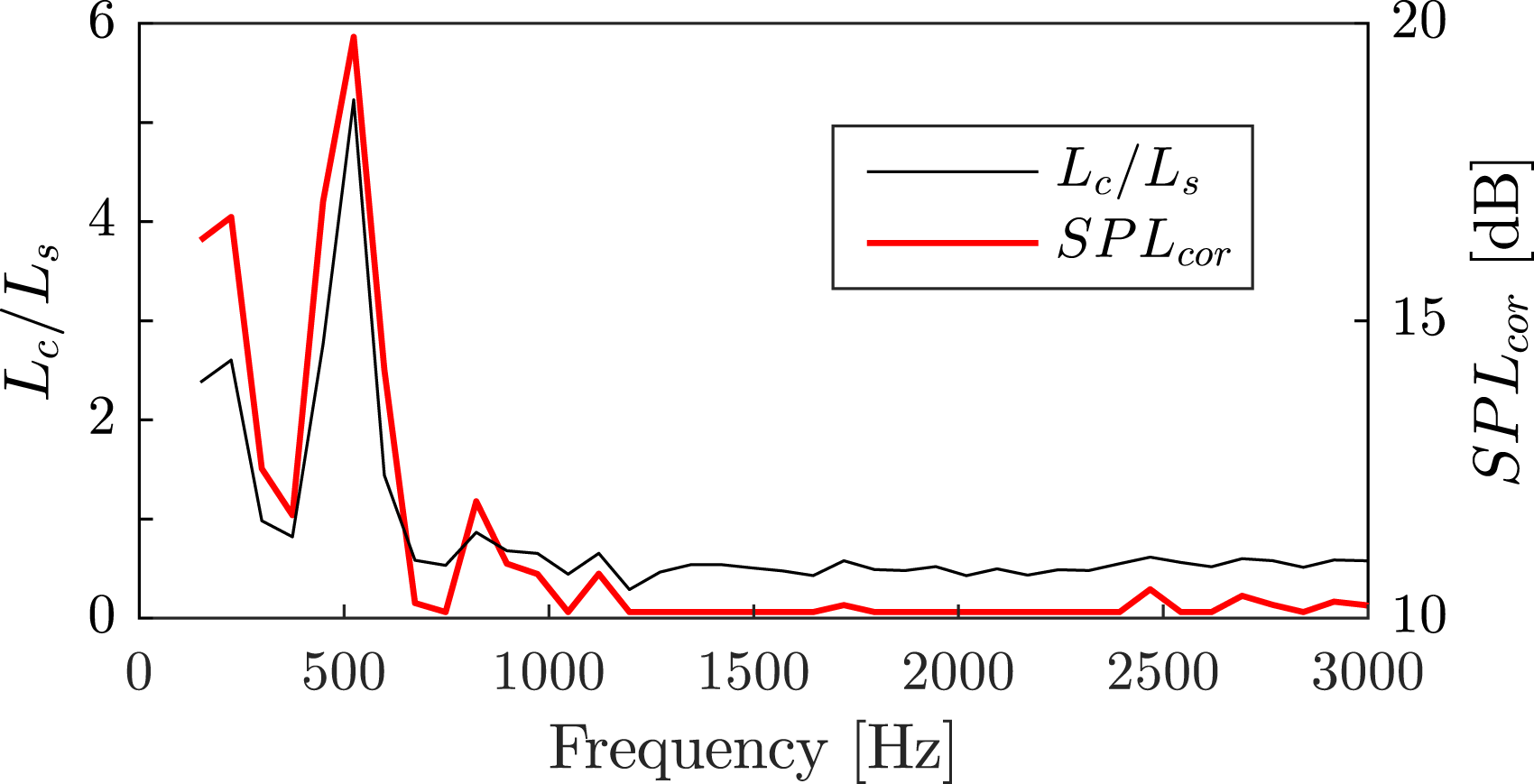

Verification for spanwise correction

It is validated in this section that the spanwise correction method is applicable to the present spanwise domain size. The correction cannot be appropriately made if the simulated spanwise extent is too limited compared to the characteristic length of large shedding vortices. The results from the cases listed in Table 1 are presented, which are CASE B with the same domain size L_s = 0.4c as the reference case and CASE D with a three times larger size L_s = 1.3c.

The correction is applied in the same way, that is, the span of airfoil is divided into 5 subsections, and the coherence is obtained from the average of 8 spectra. The resolution of frequency is 19 Hz and 51 Hz for CASE B and CASE D, respectively. Figure 11 shows the sound pressure level for correction as a function of frequency for both two cases. The minimum and maximum values of SPL_cor are 10.1 dB and 20.2 dB for CASE B, and 5.3 dB and 10.7 dB for CASE D. The sound pressure level for correction normalized with the range between these minimum and maximum values, ${SPL}_{c o r}^{*}$ , is used to plot Figure 11. The values of ${SPL}_{c o r}^{*}$ are close between the two cases at 500 Hz, but relatively large differences are observed at lower frequencies. Thus, the spanwise domain size L_s = 0.4c may not be sufficient if low frequency components need to be corrected highly accurately.

Figure 11.

1/3 octave band spectra for the SPL simulated using the span length L_s = 0.4c (CASE B, red dotted) and 1.3c (CASE D, blue solid line) observed at 1.2 m from the trailing edge with reference to 2 × 10⁻⁵ Pa. Both SPL before (bold) and after (thin line) correction are shown for each case.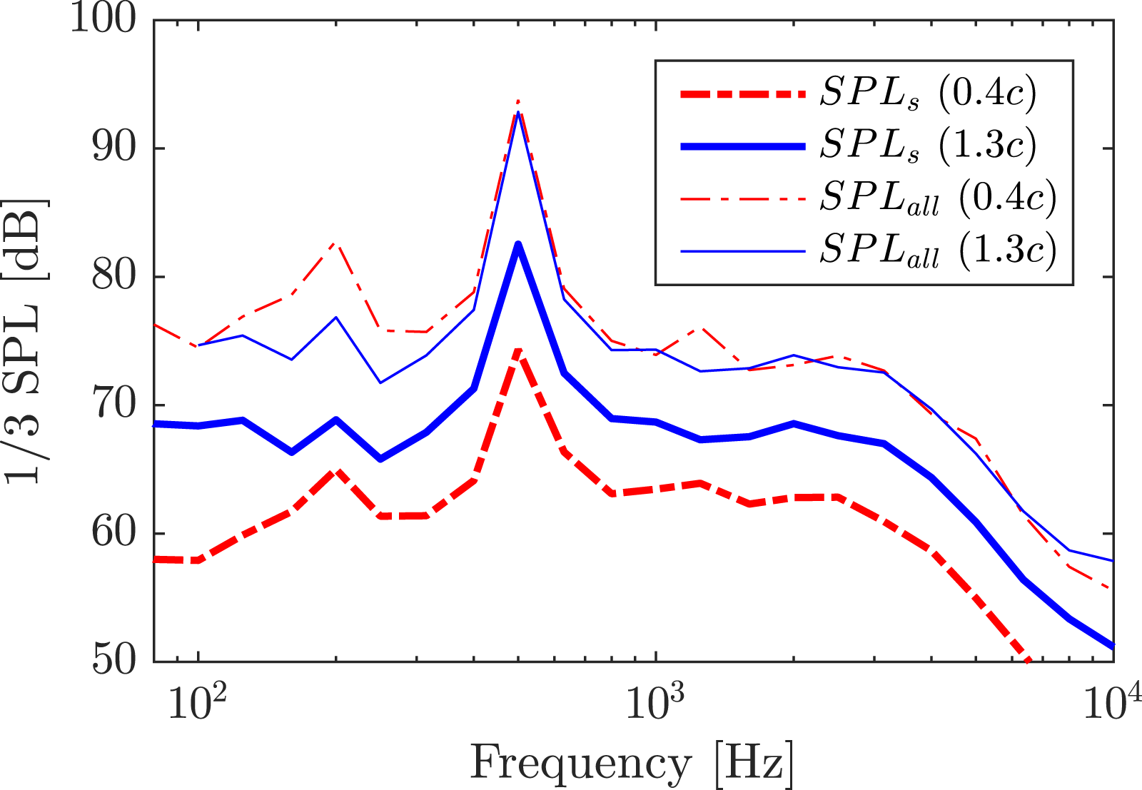

Figure 12 shows the SPL represented with two curves for CASE B (red dotted) and with two other curves for CASE D (blue solid line). Among these four curves, the upper two thin ones corresponds to SPL_all and the lower two bold ones corresponds to SPL_s. The SPL is presented as one-third octave band spectrum with reference pressure p_ref for this and all figures that follow. The values of SPL_all for the two cases are close in the range of frequencies higher than 400 Hz, and the difference is less than 2 dB, except for at 1250 Hz where the difference is 4 dB. Thus, the dimension of the spanwise domain L_s = 0.4c can be considered to be sufficient to reproduce the total SPL radiated from section L with reasonable accuracy in the main frequency range.

Figure 12.

Spectra of the corrected SPL for the symmetry and periodic boundary conditions simulated using the span length L_s = 0.4c and 1.3c.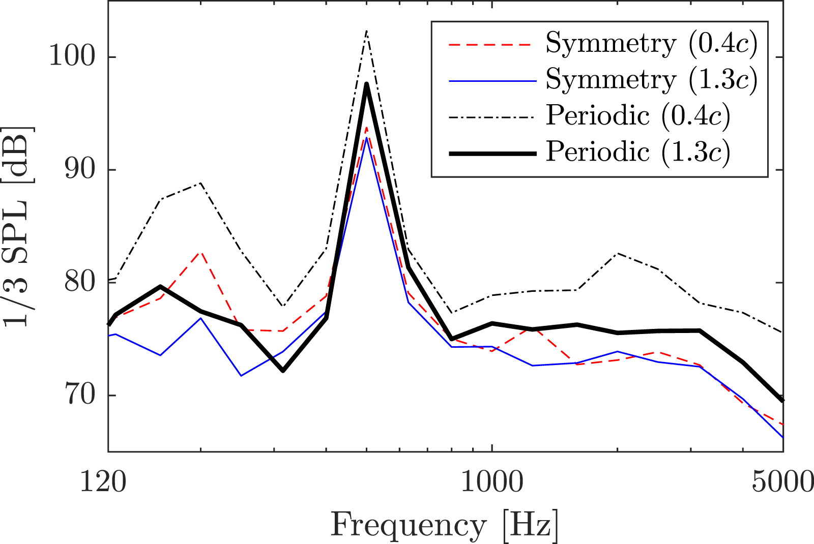

It is noted that this verification almost covers the possible range of SPL_cor, as SPL_cor has frequency components of both high and low correlation. SPL_cor is 19 dB and 10 dB at 500 Hz for CASE B and CASE D. Both values are almost the maximum of SPL_cor and thus the flow field is considered to be strongly correlated at this frequency. SPL_cor is around the minimum value for both cases at frequencies higher than 1000 Hz where the flow structure has little correlation.

The large discrepancy is seen at frequencies around 200 Hz, which can be considered to arise because of the finite computational domain. The flow cannot go through and is reflected at the boundaries in the y direction when the slip condition is applied, and this creates spurious sound waves. There is a peak at 200 Hz in both two cases, but the level in CASE D is lower than that in CASE B by 6 dB. This fact could endorse the possibility of these boundary effects. This might be reduced for instance by using non-reflecting boundary conditions, which will be addressed in a future study.

The spanwise correction has been applied in other applications using CFD simulations, as can be seen in some works by Moon et al.³³ for a flat plate and by Orselli et al.³⁴ for a circular cylinder, where the noise source causing the main tonal noise is attributed to the vortex shedding in the wake. The coherence length at the vortex-shedding frequency is several times larger than the spanwise domain size in their studies as well as in this study (see Figure 10), and they found that the tonal peak in the SPL spectrum is predicted well. It can be expected that the correction method will be applicable as long as the coherence length is appropriately estimated.

Influence of boundary condition

Both the symmetry and periodic conditions are tested to investigate whether the boundary condition in the spanwise direction affects the noise prediction. In addition to CASE B and CASE D, the results of two other cases, CASE C and CASE E, are presented in this section. The spanwise correction is applied in the same manner for all the cases.

Figure 13 shows the spectra of SPL_all obtained by the spanwise correction for all the four cases, that is, the cases simulated using the symmetry and periodic conditions with L_s = 0.4c and 1.3c. Unlike the symmetry cases, the spectra of the two periodic cases do not converge to values close to each other. This indicates that the domain size in the spanwise direction does affect the flow properties related to acoustic sources, so a longer span length might be necessary to be acoustically independent from boundaries when the periodic condition is applied.

Figure 13.

1/3 octave band spectra for the SPL predicted by LES and measured by Brooks et al.³ that is observed at 1.2 m from the trailing edge with reference to 2 × 10⁻⁵ Pa. The SPL corrected with fully coherent and incoherent assumptions are presented as well with upper and lower dotted lines.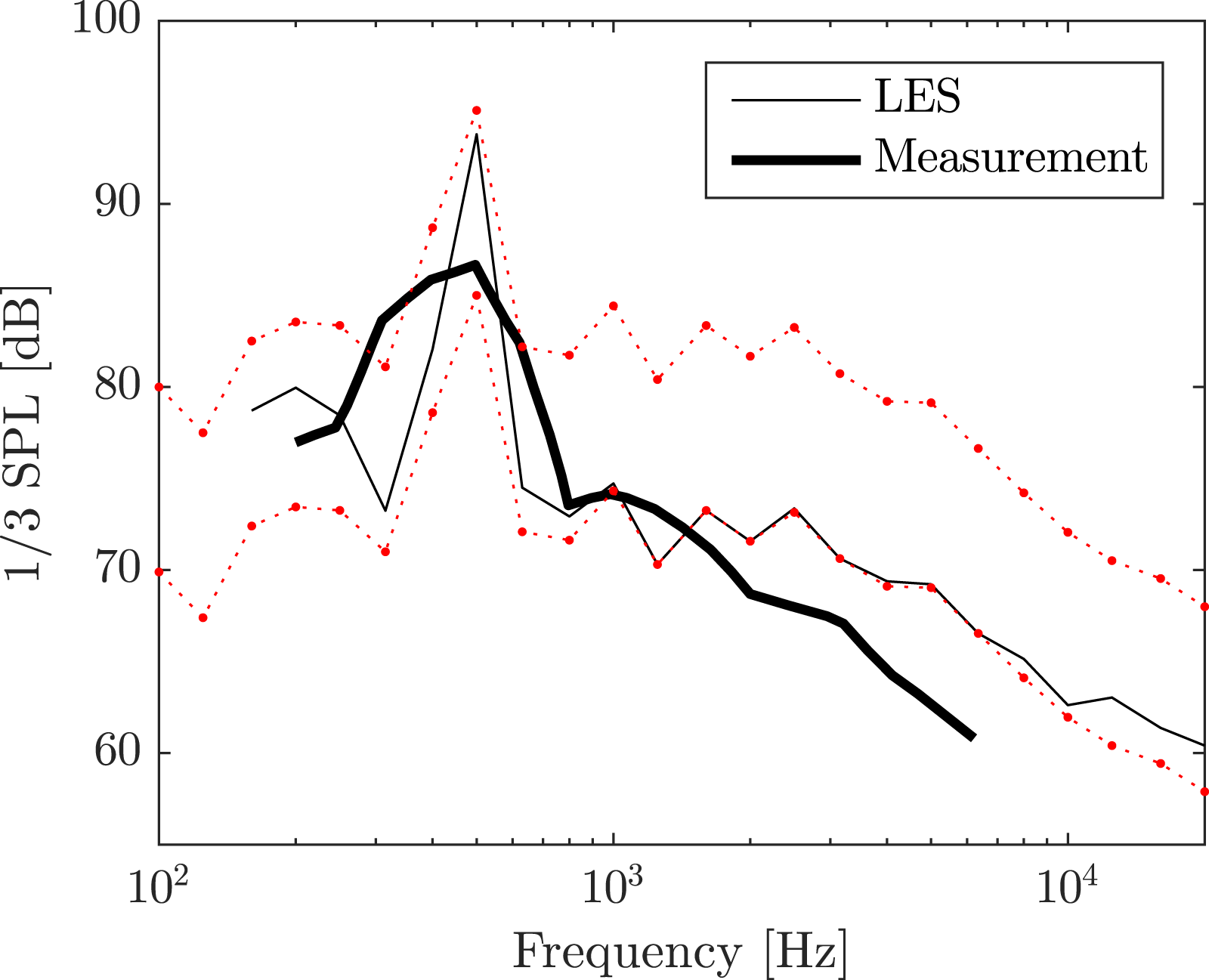

Some studies mention the influence of the boundary conditions in the spanwise direction on the airfoil noise prediction. Christophe et al.¹⁰ predicted the airfoil noise using the symmetry and periodic boundaries and found that each boundary condition showed different spanwise coherence behavior. Boudet et al.⁵ stated that the slip condition better represents the physical phenomenon, as periodicity conditions fully correlate all the flow quantities but the slip condition only imposes one component of velocity in the spanwise direction. The periodic condition could be sensitive to the spanwise dimension and overpredict the noise if the span length is too limited compared to the size of characteristic flow features, and careful attention should be paid to selection of the domain size.

Comparison with measurement

Figure 14 shows a comparison between the SPL predicted by LES and measured by Brooks et al.³ that is observed at 1.2 m from the trailing edge in the direction perpendicular to the freestream velocity in the midspan plane. The values of SPL_all corrected with the maximum and minimum values of SPL_cor, which correspond to the first and last expressions in equation (8) respectively, are also presented with two dotted lines in the figure. Overall, the predicted SPL agrees with measurement with a discrepancy of a few decibels. As shown in Figure 10, the corrected SPL becomes close to the maximum at 500 Hz and almost minimum at frequencies higher than 1000 Hz. The LES is able to predict the frequency of the main peak at 500 Hz but does not reproduce the shape of the moderate hump highly accurately. Singer et al.³⁵ stated in their airfoil noise study that the spectrum of surface pressure is dominated by the peaks at the vortex-shedding frequency and its harmonics when the grid resolution is low, but increasing the resolution fills the spectrum more fully. Thus, this discrepancy might be improved by using a finer mesh around airfoil. Although there is a distinctive frequency of the surface pressure at 2913 Hz in the half front of the airfoil observed in Figure 7, this high frequency component does not seem to yield a noticeable noise level in this sound pressure spectrum.

Figure 14.

Directivity pattern of the overall SPL at a radial distance of 1.2 m from the trailing edge.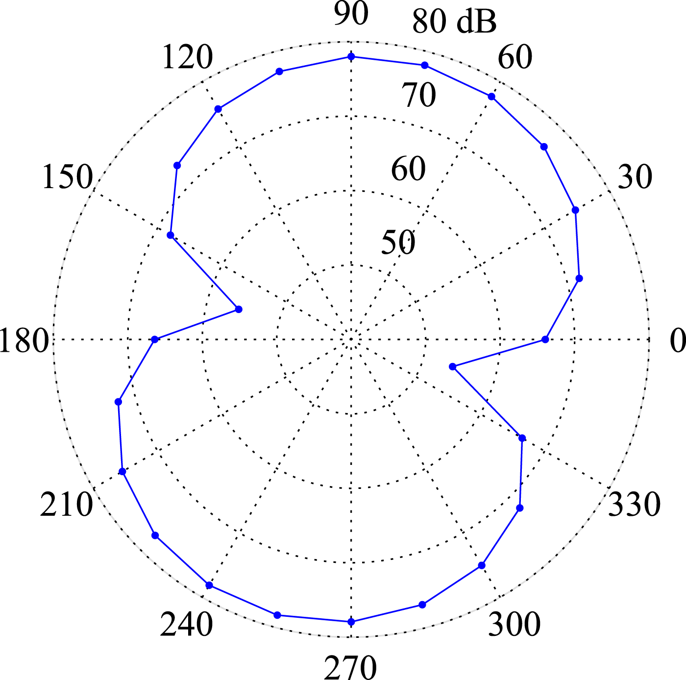

Directivity pattern

Figure 15 shows the directivity of the overall SPL observed at a radial distance of 1.2 m from the trailing edge for every 15° azimuth angle. The values presented are calculated from the SPL radiated from the simulated span section, so no spanwise correction is applied. The predicted directivity depicts the dipole source behavior, which is typical for the radiation of the trailing-edge noise. It is symmetry about the line with 15° angle, and the amplitude is close between the opposite two sides. The maximum amplitude is observed in the direction of 75° and 255° on each side. Since the compact source is assumed in the acoustic calculation, a complicated pattern which would be caused by noncompact sources of high frequencies is not present in this result.

Conclusion

In this article, the aeroacoustic noise is predicted for a NACA 0012 airfoil in stall condition using LES and the acoustic analogy. To validate the prediction, the condition measured for the airfoil at 15.6° angle of attack is reproduced. Since it is computationally expensive to simulate the entire span section of the airfoil, the spanwise correction is applied to predict the total sound based on the computed sound source accounting for 10% of the actual span size. The noise simulated with a three times larger span length is examined as well to verify that the spanwise correction is applicable for the present limited span length. Two different boundary conditions in the spanwise direction are also tested, and it is found that a longer span length might be needed when the periodic condition is used than when the symmetry condition is applied. While the pressure fluctuates randomly over the airfoil surface at frequencies higher than 1000 Hz, vortices periodically shed in the wake have large-scaled structure and thus cause high correlation of the surface pressure along span at the shedding frequency around 500 Hz. This is why the sound pressure level needs to be corrected properly considering the flow behavior for each frequency. The validation results show that the prediction is able to capture the frequency at the main peak caused by the shedding vortices in the wake and also that the corrected sound pressure level agrees with the measurement with a discrepancy of a few decibels. However, the calculated spectrum is more dominated by the peak than the measured one that is rather broadband around the shedding frequency. Better prediction could be achieved by using higher mesh resolution around the airfoil.

Footnotes

Acknowledegments

This work was supported by the STandUp for Energy and is part of STandUp for Wind. The authors would also like to acknowledge the financial support given by Yoshida Scholarship Foundation for the duration of this research activity. The computations were enabledby resources provided by the Swedish National Infrastructure for Computing (SNIC) at NSC at Linköping University partially funded by the Swedish Research Council through grant agreement no. 2020/5-321.

Declaration of Conflicting Interests

The author(s) declared no potential conflicts of interest with respect to the research, authorship, and/or publication of this article.

Funding

The author(s) received no financial support for the research, authorship, and/or publication of this article.

ORCID iD

Aya Aihara

References

Paterson

Vogt

Fink

, et al. Vortex noise of isolated airfoils. J Aircraft 1973; 10(5): 296–302.

Arbey

Bataille

. Noise generated by airfoil profiles placed in a uniform laminar flow. J Fluid Mech 1983; 134: 33–47.

Brooks

Pope

Marcolini

. Airfoil self-noise and prediction. NASA Langley Research Center: NASA Reference Publication No. 1218, 1989.

Desquesnes

Terracol

Sagaut

. Numerical investigation of the tone noise mechanism over laminar airfoils. J Fluid Mech 2007; 591: 155–182.

Boudet

Grosjean

Jacob

. Wake-airfoil interaction as broadband noise source: a large-eddy simulation study. Int J Aeroacoustics 2005; 4(1-2): 93–115.

Wang

Moin

. Computation of trailing-edge flow and noise using large-eddy simulation. AIAA J 2000; 38(12): 2201–2209.

Manoha

Herrero

Ben Khelil

, et al. Numerical prediction of airfoil aerodynamic noise. In: 8th AIAA/CEAS aeroacoustics conference & exhibit, Breckenridge, Colorado, 17–19 June 2002.

Fink

Bailey

. Airframe noise reduction studies and clean-airframe noise investigation. NASA Langley Research Center: NASA Contractor Report No. 159311, 1980.

Suzuki

Kato

Miyazawa

, et al. Analysis of aerodynamic sound sources in a flow around a two-dimensional airfoil under stalled conditions. Trans.JSME, Ser.B 2007; 73(736): 2487–2497.

10.

Christophe

Anthoine

Moreau

. Trailing edge noise of a controlled-diffusion airfoil at moderate and high angle of attack. In: 15th AIAA/CEAS aeroacoustics conference (30th AIAA aeroacoustics conference), Miami, Florida, 11–13 May 2009.

11.

Moreau

Roger

Christophe

. Flow features and self-noise of airfoils near stall or in stall. In: 15th AIAA/CEAS aeroacoustics conference (30th AIAA aeroacoustics conference), Miami, Florida, 11–13 May 2009.

12.

Seo

Moon

. Aerodynamic noise prediction for long-span bodies. J Sound Vibration 2007; 306(3-5): 564–579.

13.

Lighthill

. On sound generated aerodynamically I. General theory. Proc R Soc Lond A 1952; 211(1107): 564–587.

14.

Curle

. The influence of solid boundaries upon aerodynamic sound. Proc R Soc Lond A 1955; 231(1187): 505–514.

15.

Larsson

Davidson

Olsson

, et al. Aeroacoustic investigation of an open cavity at low mach number. AIAA J 2004; 42(12): 2462–2473.

16.

Brentner

Farassat

. Modeling aerodynamically generated sound of helicopter rotors. Prog Aerospace Sci 2003; 39(2-3): 83–120.

17.

Lerner

Boldes

. Applied aerodynamics. Germany: BoD–Books on Demand, 2012.

18.

Glegg

Devenport

. Aeroacoustics of low Mach number flows: fundamentals, analysis, and measurement. UK: Academic Press, 2017.

19.

Wang

Freund

Lele

. Computational prediction of flow-generated sound. Annu Rev Fluid Mech 2006; 38: 483–512.

20.

Crocker

. Handbook of noise and vibration control. USA: John Wiley & Sons, 2007.

21.

Yoshizawa

. Statistical theory for compressible turbulent shear flows, with the application to subgrid modeling. Phys Fluids 1986; 29(7): 2152–2164.

22.

Harten

. High resolution schemes for hyperbolic conservation laws. J Comput Phys 1983; 49(3): 357–393.

23.

Wolf

Lele

. Trailing-edge noise predictions using compressible large-eddy simulation and acoustic analogy. AIAA J 2012; 50(11): 2423–2434.

24.

Moreau

Christopher

Roger

M. LES

of the trailing-edge flow and noise of a NACA0012 airfoil near stall. In: Proceedings of the CTR summer program, Stanford, California, 24 June–20 July 2018, pp. 317–329.

25.

Kato

Iida

Takano

, et al. Numerical prediction of aerodynamic noise radiated from low mach number turbulent wake. In: 31st Aerospace sciences meeting, Reno, Nevada, 11–14 January 1993.

26.

Pérot

Gloerfelt

Bailly

, et al. Numerical prediction of the noise radiated by a cylinder. In: 9th AIAA/CEAS aeroacoustics conference and exhibit, Hilton Head, South Carolina, 12–14 May 2003.

27.

Jacob

Boudet

Casalino

, et al. A rod-airfoil experiment as a benchmark for broadband noise modeling. Theor Comput Fluid Dyn 2005; 19(3): 171–196.

28.

Menter

Kuntz

Langtry

. Ten years of industrial experience with the SST turbulence model. Turbulence, Heat and Mass Transfer 2003; 4(1): 625–632.

29.

Moreau

Henner

Iaccarino

, et al. Analysis of flow conditions in freejet experiments for studying airfoil self-noise. AIAA J 2003; 41(10): 1895–1905.

30.

Brooks

Marcolini

Pope

. Airfoil trailing-edge flow measurements. AIAA J 1986; 24(8): 1245–1251.

31.

Aihara

Goude

Bernhoff

. LES prediction for acoustic noise of airfoil at high angle of attack. In: AIAA scitech 2020 forum.

32.

Michos

Bergeles

Athanassiadis

. Aerodynamic characteristics of NACA 0012 airfoil in relation to wind generators. Wind Eng 1983; 7(4): 247–262.

33.

Moon

Seo

Bae

, et al. A hybrid prediction method for low-subsonic turbulent flow noise. Comput Fluids 2010; 39(7): 1125–1135.

34.

Orselli

Meneghini

Saltara

. Two and three-dimensional simulation of sound generated by flow around a circular cylinder. In: 15th AIAA/CEAS aeroacoustics conference. (30th AIAA aeroacoustics conference), Miami, FL, 11–13 May 2009.

35.

Singer

Brentner

Lockard

, et al. Simulation of acoustic scattering from a trailing edge. J Sound Vibration 2000; 230(3): 541–560.

Numerical prediction of noise generated from airfoil in stall using LES and acoustic analogy

Abstract

Keywords

Introduction

Computational method

Acoustic prediction

Aerodynamic calculation

Spanwise correction

Study cases

Results and discussion

Flow characteristics

Acoustic calculation

Procedure for spanwise correction

Verification for spanwise correction

Influence of boundary condition

Comparison with measurement

Directivity pattern

Conclusion

Footnotes

Acknowledegments

Declaration of Conflicting Interests

Funding

ORCID iD

References