Sage Journals: Discover world-class research

Abstract

This study investigates the numerical prediction for the aerodynamic noise of the vertical axis wind turbine using large eddy simulation and the acoustic analogy. Low noise designs are required especially in residential areas, and sound level generated by the wind turbine is therefore important to estimate. In this paper, the incompressible flow field around the 12 kW straight-bladed vertical axis wind turbine with the rotor diameter of 6.5 m is solved, and the sound propagation is calculated based on the Ffowcs Williams and Hawkings acoustic analogy. The sound pressure for the turbine operating at high tip speed ratio is predicted, and it is validated by comparing with measurement. The measured spectra of the sound pressure observed at several azimuth angles show the broadband characteristics, and the prediction is able to reproduce the shape of these spectra. While previous works studying small-scaled vertical axis wind turbines found that the thickness noise is the dominant sound source, the loading noise can be considered to be a main contribution to the total sound for this turbine. The simulation also indicates that the received noise level is higher when the blade moves in the downwind than in the upwind side.

Keywords

Vertical axis wind turbine acoustics aerodynamic noise CFD LES

Introduction

The wind is an alternative clean energy resources, and the total number of installed wind turbines has continued to increase the last decades. However, noise emission from operating wind turbines is one of the issues which restrict the siting, and noise annoyance to nearby residents still has been a problem.^1,2 Therefore, it is important to estimate the noise level of wind turbines and optimize the design to reduce the noise immission.

Noise generated from wind turbines can be classified into mechanical noise and aerodynamic noise. The mechanical noise originates from machinery components, such as a gearbox, generator, and yaw drives. Aerodynamic noise is radiated from the blades and is mainly associated with the interaction of turbulence with the blade surface. The turbulence may originate either from the natural atmospheric turbulence present in the incoming flow or from the viscous flow in the boundary layer around the blades.³ Since some decades, manufacturers have been able to reduce the mechanical noise to a level below the aerodynamic noise, now creating the situation that aerodynamic noise is the dominant noise mechanism.³

The aerodynamic noise can be divided into low frequency noise, inflow turbulence noise, and airfoil self-noise. The low frequency noise is generated when the rotating blade experiences changes in the flow by some factors, such as the presence of the tower, wind speed fluctuation, and wakes from other blades. The most important mechanism of low frequency noise for horizontal axis wind turbines (HAWTs) is interaction with the tower that creates periodic flow disturbances during rotation. Vertical axis wind turbines (VAWTs) experience less tower interference as the distance between blades and the tower is much larger.⁴ The characteristic frequency range of low frequency noise from wind turbines is from about 10 to 200 Hz.⁵ The inflow turbulence noise is created when the upstream flow encounters the blades, therefore it depends on the amount of turbulence in the atmospheric flow. This interaction radiates a broadband noise. The airfoil self-noise, which has both tonal and broadband character, can be linked to several phenomena caused by the aerodynamic behavior in the boundary layer around the airfoil surface. Brooks et al.⁶ identified the mechanisms of airfoil noise as five sources: boundary layer turbulence passing the trailing edge, separated-boundary-layer and stalled-airfoil flow, vortex shedding due to laminar-boundary-layer instabilities, vortex shedding from blunt trailing edges, and the turbulent vortex flow existing near the blade tips.

The dominant sound source can differ depending on the rotor scale. For small and medium-sized turbines, where Re < 10⁶, the laminar-boundary-layer vortex-shedding noise can become important, whereas it can be neglected for modern large turbines.³ The H-rotor VAWT has the advantage that it generates less noise than a HAWT.⁴ VAWTs have a wide range of sizes, and therefore different dominant sound sources have been found for various turbines by some studies. Pearson⁷ stated for a small-scaled 7.5 kW rotor that the laminar-boundary-layer tonal noise is a significant source and the inflow turbulence has very little effect at high tip speed ratio. On the contrary, Ottermo et al.⁸ and Möllerström et al.⁹ studied for a 200 kW VAWT whose Reynolds number is of the order of 10⁶⁹ and stated that the noise originates predominantly from the turbulent inflow.

Due to the demand of reducing the noise generated from wind turbines, several researchers^10–12 have established approaches based on semi-empirical models for predicting wind turbine aerodynamic noise. Empirical models are commonly assuming independently generated noise sources.¹³ These models are developed for a single two-dimensional airfoil, for instance, based on the experimental database by Brooks, Pope and Marcolini,⁶ and the total sound pressure level of a wind turbine is calculated by summing all the predicted sound sources of each blade segment. For example, Moriarty and Migliore¹³ developed the code and validated against measurements for a full-scaled wind turbine. Zhu et al.¹⁴ and Leloudas et al.¹⁵ developed an empirical model to calculate the noise from large-scaled wind turbines and compared with measurements. Rasam et al.¹⁶ and Botha et al.^{17, 18} applied empirical models to predict sound for both horizontal and vertical axis wind turbines and compared two different approaches using computational fluid dynamics (CFD) and analytical methods. Sucameli¹⁹ assessed the noise radiated from a 3.6 MW wind turbine using an empirical model considering the trailing edge and inflow turbulence noise. These empirical methods are efficient in computing speed but have limitations in capturing three-dimensional effects.¹²

Recently, solving a wall-bounded flow field using CFD simulations is becoming an alternative for predicting noise sources and there are some works calculating the noise of wind turbines. Mohamed²⁰ performed two-dimensional Reynolds averaged Navier-Stokes (RANS) simulations to examine the dependence of the noise for Darrieus wind turbines on different blade shapes, tip speed ratios, and solidity. Wasala et al.²¹ carried out large eddy simulation (LES) to predict the noise for a 600 kW HAWT using the acoustic analogy. They showed that the leading edge noise is the predominant noise source in a highly turbulent environment. Tadamasa et al.²² predicted the noise radiated from the 20 kW two-bladed HAWT using three-dimensional RANS simulations which are used for inputs to the acoustic analogy codes. It was found that the loading noise is the dominant noise source until about the rotational speed of 130 rpm, which can be considered as relatively high TSR, but the thickness noise becomes dominant for higher rotational speed. Ghasemian and Nejat²³ conducted the incompressible LES to predict aerodynamic noise radiated from the VAWT by simulating for 1/7 of the blade span section. They showed that the rotational speed determines the strength of radiated noise and also that the sound pressure level (SPL) spectra have clear peaks at the rotational frequency. In order to predict the noise for the H-Darrieus wind turbine, Weber et al.⁵ validated the numerical methods based on an extended RANS model using two different aeroacoustic approaches. They concluded that the main noise source for the condition operated at low tip speed ratio is caused due to dynamic stall of the blades and the interaction with vortices generated from the blades in the upwind.

This study predicts the aerodynamic noise of a 12 kW VAWT using LES and the acoustic analogy, and the predicted SPL is compared to measurement data. The H-rotor VAWT which has the rotor diameter of 6.5 m and three blades of 5 m height is studied in this paper. The prediction is made for the turbine operating at high tip speed ratio where the turbine is expected to produce more noise than at low tip speed ratio.²⁴ The CFD model includes the strut components as well, which are mounted with an angle and thus give a more prominent contribution to the turbine aerodynamics. In addition, the blade-strut joints create high turbulence that can in turn produce a noise contribution, as shown in the sound source maps measured by Ottermo et al.⁸

This article is organized in two parts: first, the numerical model is validated for a single static airfoil case using the acoustic measurement conducted by Brooks et al.⁶ It is also validated for the aerodynamics of the VAWT by comparing measurement by Li et al.²⁵ Next, the prediction and the measurement is compared to validate the accuracy of the numerical model. The simulated sound pressure is examined further in detail to investigate the mechanism of noise generation for this turbine.

Acoustic calculation

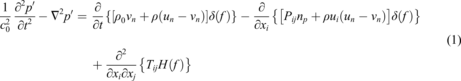
In this article, the Ffowcs Williams and Hawkings (FW-H) equation²⁶ is used to predict the acoustic noise. Lighthill^27,28 first derived the acoustic wave equation by rearranging the Navier-Stokes equations with the aim of analyzing the aircraft jet noise. The FW-H equation is an extension of the equation developed by Lighthill and describes the sound generated by a body moving in a fluid represented as a moving control surface.

Let us denote the sound pressure as p^′ = p−p₀, which is the deviation from the ambient pressure p₀. The subscript ₀ defines the values in the undisturbed medium, and the same applies to the speed of sound c and the density of a fluid ρ. The FW-H equation for p^′ is written as

\begin{array}{l} \frac{1}{c_{0}^{2}} \frac{\partial^{2} p^{'}}{\partial t^{2}} - \nabla^{2} p^{'} = \frac{\partial}{\partial t} {[ρ_{0} v_{n} + ρ (u_{n} - v_{n})] δ (f)} \\ - \frac{\partial}{\partial x_{i}} {[P_{i j} n_{p} + ρ u_{i} (u_{n} - v_{n})] δ (f)} \\ + \frac{\partial^{2}}{\partial x_{i} \partial x_{j}} {T_{i j} H (f)} \end{array}

(1)

where n_p is the unit vector normal to the surface, u_i is the fluid velocity in the i direction, u_n is the fluid velocity in the direction normal to the surface, v_n is the velocity of the surface, δ(f) is the Dirac delta function, H(f) is the Heaviside function, respectively. The shape and the motion of the control surface is described using f, that is, f > 0 implies outside the surface, f = 0 the body surface, and f < 0 inside the surface. The Lighthill stress tensor T_ij is expressed as

T_{i j} = ρ u_{i} u_{j} + P_{i j} - c_{0}^{2} (ρ - ρ_{0}) δ_{i j}

(2)

where P_ij is the compressive stress tensor that includes the surface pressure and the viscous stress. The first term on the right hand side of equation (1) relates the monopole type source, and the thickness noise is attributed to this source. The second term relates the dipole type source, and the loading noise originates from this term. The third term relates the quadrupole type source.

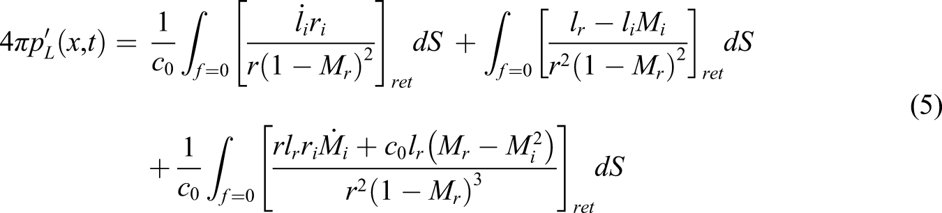
The solution for the FW-H equation can be obtained using the free space Green’s function. The sound pressure at a receiver position can be written as the summation of the thickness and loading noise.

p^{'} = p_{T}^{'} + p_{L}^{'}

(3)

The thickness noise

p_{T}^{'}

\begin{array}{l} 4 π p_{T}^{'} (x, t) = \int_{f = 0} {[\frac{ρ_{0} (\dot{v_{n}} n_{p} + v_{n} \dot{n_{p}})}{r {(1 - M_{r})}^{2}}]}_{r e t} d S \\ + \int_{f = 0} {[\frac{ρ_{0} v_{n} n_{p} {r r_{i} \dot{M_{i}} + c_{0} (M_{r} - M_{i}^{2})}}{r^{2} {(1 - M_{r})}^{3}}]}_{r e t} d S \end{array}

(4)

and the loading noise

p_{L}^{'}

\begin{array}{l} 4 π p_{L}^{'} (x, t) = \frac{1}{c_{0}} \int_{f = 0} {[\frac{\dot{l_{i}} r_{i}}{r {(1 - M_{r})}^{2}}]}_{r e t} d S \\ + \int_{f = 0} {[\frac{l_{r} - l_{i} M_{i}}{r^{2} {(1 - M_{r})}^{2}}]}_{r e t} d S \\ + \frac{1}{c_{0}} \int_{f = 0} {[\frac{r l_{r} r_{i} \dot{M_{i}} + c_{0} l_{r} (M_{r} - M_{i}^{2})}{r^{2} {(1 - M_{r})}^{3}}]}_{r e t} d S \end{array}

(5)

where r is the distance from the surface to the receiver, r_i is the unit vector pointing from the source location to the receiver, l_i = p_ijn_p is the pressure vector exerted by fluid on the surface, l_r = r_il_i is the component of l_i in the direction of radiation, M_i = v_n/c₀ is the Mach number at a point on the surface, M_r = r_iv_n/c₀ is the Mach number in the direction of radiation. The subscript ret denotes that the integrand is evaluated at the retarded time τ defined as

τ = t - \frac{r}{c_{0}}

(6)

where t is receiver time. The detailed procedure of the derivation is described in reference.²⁹

The study case is in low Mach number regime. The quadrupole source is neglected because its contribution to the total sound is generally expected to be much smaller than that of the monopole and dipole sources for low Mach number flows.³⁰ It is also assumed that the sound source can be regarded as compact in the range of dominant frequencies due to the low Mach number flow.

Turbine geometry

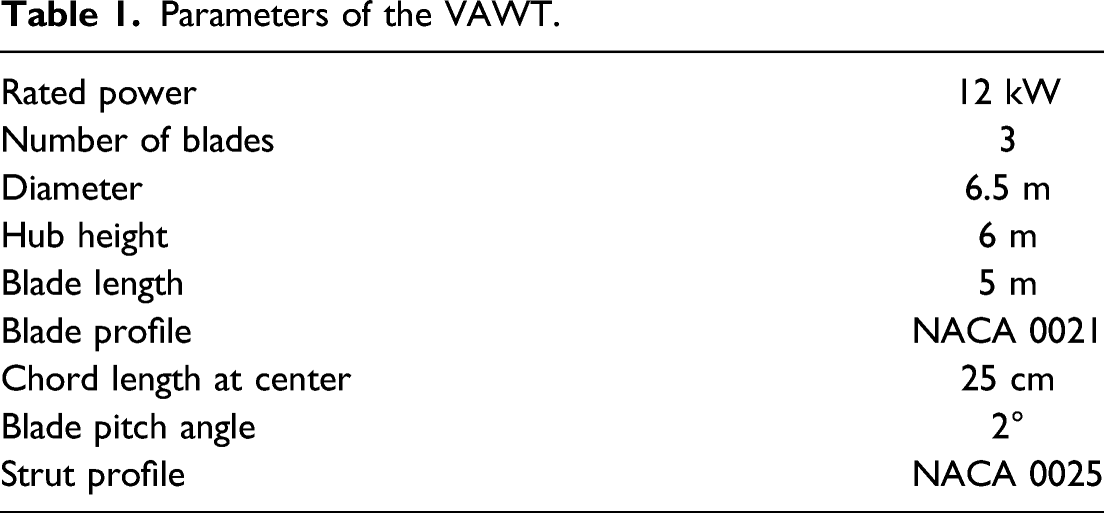
Figure 1 shows the VAWT located at Marsta in Sweden, which has been designed and built by the Division of Electricity at Uppsala University. The main parameters of the geometry are listed in Table 1. The radius of the rotor is R = 3.24 m, and the hub is located at 6 m from the ground. It consists of three blades which have the cross-sectional profile of a NACA 0021 airfoil. Each blade has a length of 5 m. The chord length is c = 25 cm, and it is tapered on both sides, starting from 1 m from the blade tip, with the chord linearly decreasing to 15 cm at the tip. The Reynolds number based on chord length varying during revolution is in the order of 10⁵. Two inclined struts are attached to each blade at 27% of the blade length from the tip. The cross-section of the struts is designed based on a NACA 0025 profile but with modification at the trailing edge to have a blunt edge. The chord length Varies linearly from 32 cm at the root up to 20 cm at the attachment point. A detailed description of the strut geometry can be referred to Goude and Rossander.³¹

Figure 1.

12 kW vertical axis wind turbine.

Table 1.

Parameters of the VAWT.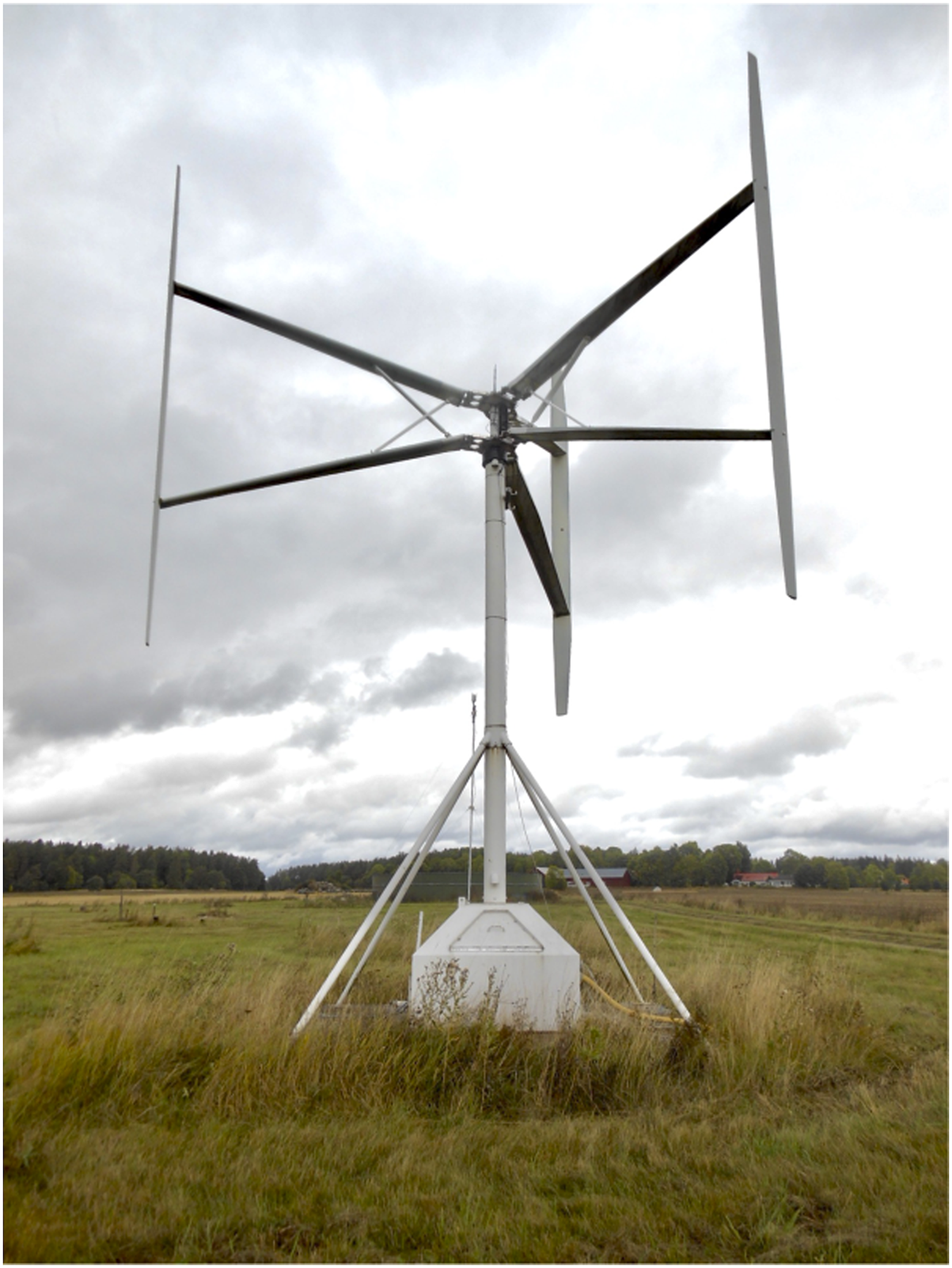

Rated power	12 kW
Number of blades	3
Diameter	6.5 m
Hub height	6 m
Blade length	5 m
Blade profile	NACA 0021
Chord length at center	25 cm
Blade pitch angle	2°
Strut profile	NACA 0025

The turbine rotates with an angular velocity ω, and the azimuth angle is denoted by θ. The value of θ is 0 when the blades move toward the freestream wind (see Figure 3). The tip speed ratio is defined as Rω/U_∞ where ω is an angular velocity and U_∞ is the freestream velocity at hub height. The average values for U_∞ and ω during the recording time period are 3.7 m/s and 49.1 rpm, respectively. The tip speed ratio used in the simulation is 4.47, which is considered to be high for this turbine.

Acoustic measurement

The measurements were performed between 14:20 and 14:50 on September in 2020. The wind came mostly from the South direction. The temperature was around 17°C. The sound was measured with a Class 1 Sound Level Meter (Brüel and Kjær 2270) and calibrated prior to each new measurement position using a Larson-Davis CAL200 calibrator at 94 dB. The microphone was mounted at 1.2 m height as shown in Figure 2, and it was horizontal and directed toward the wind turbine. Reported numbers are 1 min equivalent sound levels from each position, and this time period approximately corresponds to time of 50 revolutions of the rotor. The background sound, that is, sound not from the wind turbine, was originating from a road at 1 km distance to the East of the wind turbine site and also occasionally propeller aircraft from a nearby airstrip was observed. During all the reported measurements, the background sound levels were low and the reported sound levels are considered by the authors to be originating from the wind turbine.

Figure 2.

Microphone.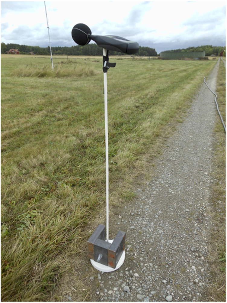

Figure 3 shows the locations where the sound was recorded. It was recorded for eight and four azimuthal directions at the radial distances of 1.4D and 2.8D, and these locations are arranged at every 45° and 90° with all positions shifted clockwise by 15° from the averaged incoming wind direction, respectively.

Figure 3.

Locations of sound observation.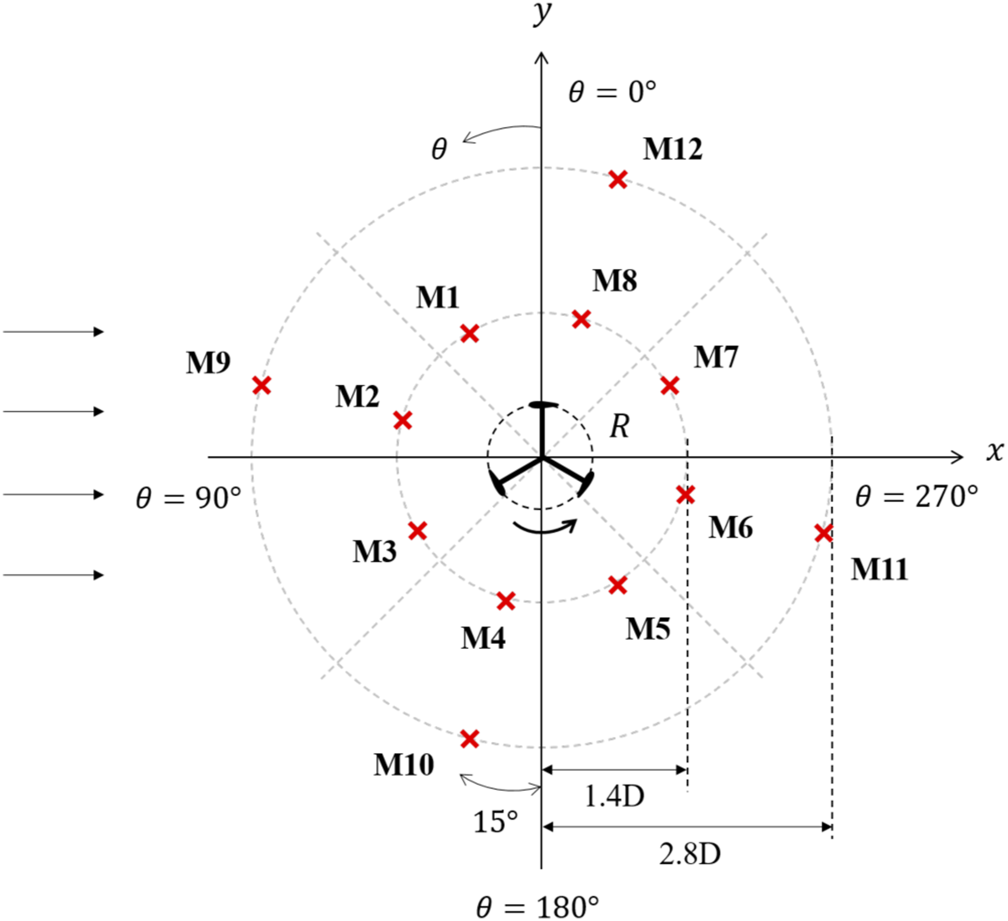

There exist uncertainties in acoustic measurements due to the directional variability using a microphone, and they should mainly be due to two factors. The first factor is different reflections of the ground. The sound reflected on the ground should be similar for all different measurements as the ground was covered with the same type of grass for all measurement positions. Therefore, the uncertainty due to this factor should rather be the same bias for all positions. The second factor is turbulent fluctuations during the measurement. Turbulence in the airfield will cause the sound source directivity to vary during each measurement, and the chosen duration of the measurement was set accordingly. Conclusively we consider that the uncertainties of the measurements are of comparable magnitude as a standardized IEC61400-11 procedure. Probably larger uncertainty due to not using a ground board but smaller uncertainty due to the short distance with no attenuation and perceived high S/N-ratios.

The wind speed was not perfectly constant during the measurement, and the variation of wind speed during recording time is displayed in Figure 4. The wind speed was measured by two different anemometers. One anemometer measures the instantaneous wind at hub height every minute which is shown with a solid line. The other one measures the 10-min average wind at 4 m height, and these values, as shown with markers, are corrected to the wind speed at hub height using equation (7). The dashed line represents the mean value which is used in the simulation.

Figure 4.

Wind speed at hub height recorded by two different anemometers during the entire measurement time with the average wind speed value used in simulation represented by the dashed line.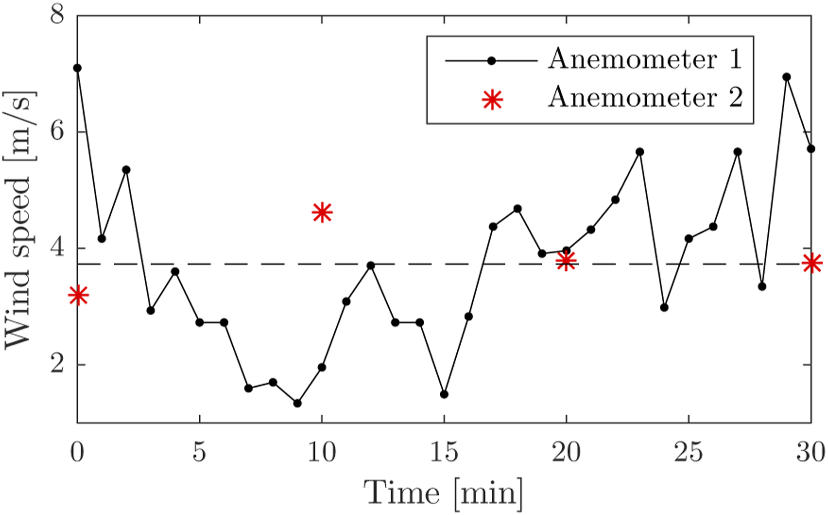

Numerical approach

In order to compute the sound source around the VAWT, incompressible flow simulations are performed using the open source code OpenFOAM,³² which solves the continuity and momentum equations based on the finite volume method. The flow field is solved using LES with the WALE (Wall Adapting Local Eddy-viscosity) SGS model.³³ This model is based on the square of the velocity gradient tensor and can perform well for the flow with transition from laminar to turbulent flows.³⁴

The PIMPLE algorithm developed for transient problems is applied to solve the coupled pressure-velocity equations. The PIMPLE algorithm is a combination of the pressure-implicit split-operator (PISO) algorithm and the semi-implicit method for pressure-linked equations (SIMPLE) algorithm. Contrary to the PISO algorithm, the PIMPLE algorithm recalculates the pressure-velocity coupling in one time step.

Time steps are adjusted so that the maximum Courant number is satisfied to be below 0.9. The time step increment is around 5.5 × 10⁻⁶ sec, which corresponds to time of rotating by azimuth angle of 0.0016°. The time derivative of pressure used in the acoustic calculation is obtained by taking a difference between two time steps. The pressure derivative is highly sensitive to the time step size, thus every ten time steps computed in the LES is extracted to use as an input to the acoustic equations. This leads to the resolved frequency up to around 9100 Hz for the calculated sound pressure.

Figure 5 shows the computational domain and the boundary conditions. The domain consists of a rotational inner part and a stationary outer part. The rotational region is represented as the circular area of 1.5D diameter. The sizes of the domain in the cross-stream and the vertical directions are 19D and 9D, and the distances from the center of rotation to the inlet and to the outlet boundaries are 10D and 19D. This domain size is considered sufficient, as Rezaeiha et al.³⁵ stated that the distance of 10D from the center to the inlet and outlet boundaries minimizes the effect of the domain.

Figure 5.

Computational domain and boundary conditions.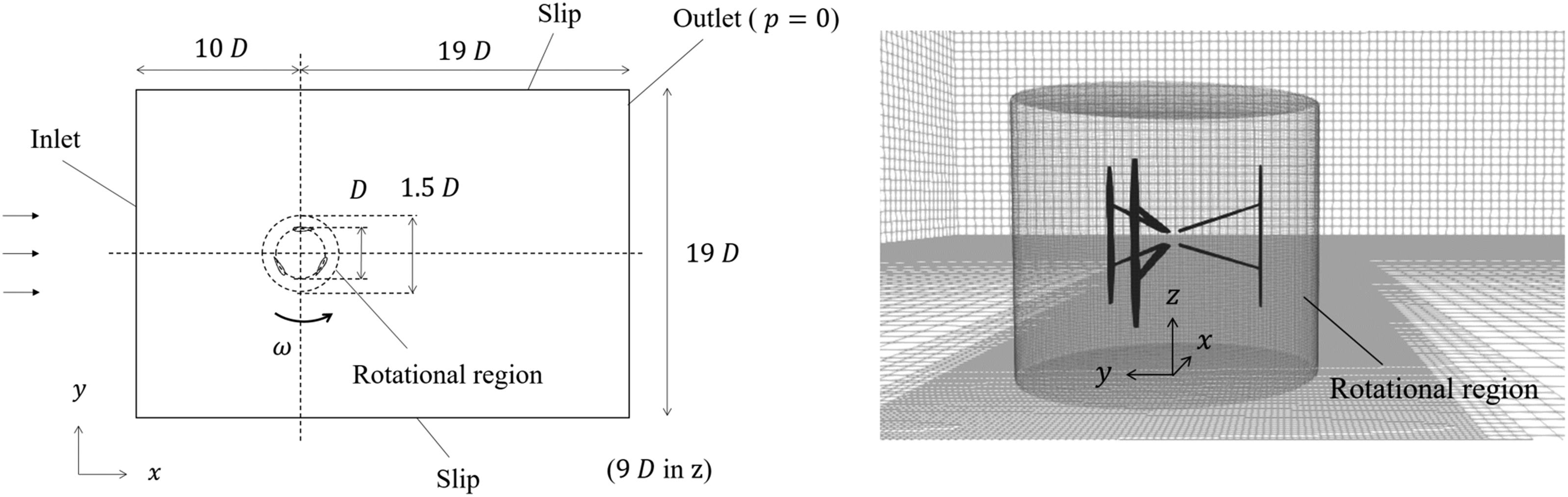

The inlet velocity is expressed by the log law. The log wind profile U_log varies with the height z and is defined as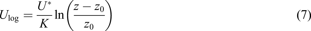

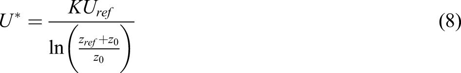
U_{\log} = \frac{U^{*}}{K} \ln (\frac{z - z_{0}}{z_{0}})

(7)

where

U^{*} = \frac{K U_{r e f}}{\ln (\frac{z_{r e f} + z_{0}}{z_{0}})}

(8)

is the frictional velocity, z₀ = 0.025 m is the roughness length, K = 0.41 is the Kármán constant. U_ref is the velocity at reference height z_ref. It is noted that only the mean flow velocity and the subgrid scale viscosity with no fluctuating velocity are imposed at inlet, although turbulent fluctuations in the inflow could affect the noise level. There is no measurement data for the atmospheric turbulence, thus it will be a future study to implement proper turbulence quantities and reproduce the actual wind condition on the site. The pressure is assumed to be zero at the outlet boundary. The slip condition is applied at boundaries in the cross-stream and the vertical directions, except for the boundary on the bottom side at z = 0 where the wall boundary conditions are used to represent the ground.

Figure 6 shows the view of the discretized mesh for the area around the blade. Only the mesh of surfaces for a single blade and two struts attached to it is refined highly finely in order to reduce the computational cost. The thickness of the first layer of this blade and two struts is less than 0.03 mm, which results in the values of y⁺ less than three over the surface.

Figure 6.

View of the mesh around the airfoil.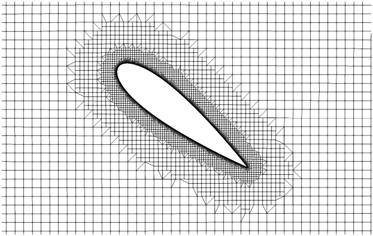

The number of total mesh cells is 50 million. The blunt edge of the blade has the size in the order of one mm and is not modeled due to high computational demand. The blunt edge of the struts is considered, as the size is a few centimeters and is relatively large compared to that of the blades. Other components such as a tower are not included, assuming that the dominant noise source is generated from the blades.

First, the steady-state flow is solved to obtain the initial fields. Then, 9 revolutions are simulated using a coarse mesh to develop the wake by a few rotor diameter distances. The last one revolution is simulated using the fine mesh to calculate the sound source.

The result data corresponding to one third of revolution are presented in the paper due to its periodicity. The sound source is computed using the simulation results from a single blade and two struts whose surfaces are finely refined. Thus, the turbine is rotated by a whole one revolution in the simulation, and the sound pressure of every one third is summed up at the end.

For the discretization of the convective terms, the first-order upwind scheme is used in the first 9 revolutions and the second-order upwind Total Variation Diminishing (TVD) scheme is used in the last revolution. In all time steps, the diffusive terms are discretized by the central difference scheme. The bounded first-order implicit scheme is used for the time differencing.

The parallel computation is run using 512 processors on the Tetralith cluster provided by the National Supercomputer Center at Linköping University. The computational domain is split into 512 subdomains, and each subdomain is assigned to one of the processors. The computational time of the last one revolution was 14.5 days.

Validation of numerical model

Static single blade

The numerical model is validated first by comparing the measurement data by Brooks⁶ for the airfoil self-noise. They conducted the acoustic test in an anechoic wind tunnel for a NACA 0012 airfoil blade section to derive the semi-empirical prediction model for the noise generation of airfoil. A study case is the data measured under the condition that the chord length is 10.16 cm, the freestream velocity is 71.3 m/s, the Reynolds number based on the chord length is 4.8 × 10⁵, and the Mach number is 0.2. The sound is received at 1.2 m perpendicular to the trailing edge of airfoil in the midspan plane.

The LES is performed using the mesh which has the same relative cell size to the chord around the airfoil. The experimental blade model has the span length of 45 cm, and the vertical dimension of the jet exit is 30.48 cm. In the measurement, two side plates are flush mounted on the jet nozzle lip and the airfoil model is held between the plates. The trailing edge of the airfoil is placed at a distance of 61.0 cm from the jet exit. The configuration of these experimental conditions including the jet exit and the side plates is reproduced in the simulation.

The SPL presented as one-third octave band spectra with reference pressure of p_ref = 2 × 10⁻⁵ Pa is shown in Figure 7 for four angles of attack, α = 0°, 5.4°, 10.8°, and 14.4°. The SPL is well reproduced for α = 10.8° and 14.4° with discrepancy of a few decibels. The agreement of the SPL for 0° and 5.4° is satisfactory up to 2000 Hz. However, the differences become critical at high frequencies. The predicted peaks at around 8000 and 6350 Hz for 0° and 5.4° are largely deviated from the measurement in terms of amplitude and frequency of the peaks. The prediction model by Brook et al.⁶ implies that the tonal noise observed in this two cases is caused mainly by the vortex shedding noise due to laminar-boundary-layer instabilities. The mechanism of the vortex shedding noise is related to the thickness of the laminar boundary layer,³⁶ and the resolution of the simulation model might not be high enough to capture this phenomenon. Another reason for these discrepancies can be that the assumption for the compactness of the sound source is not valid at high frequencies. The frequency of acoustic wavelength corresponding to the chord length is around 3400 Hz, and the sound source could not be considered compact at frequencies higher than that. It is concluded that this numerical model is able to predict the noise level at frequencies up to around 2000 Hz with reasonable accuracy but may be less reliable at higher than that.

Figure 7.

1/3 octave spectra for the predicted SPL compared to measurement by Brooks et al.⁶ observed at 1.2 m from the trailing edge with reference p_ref = 2 × 10⁻⁵ Pa.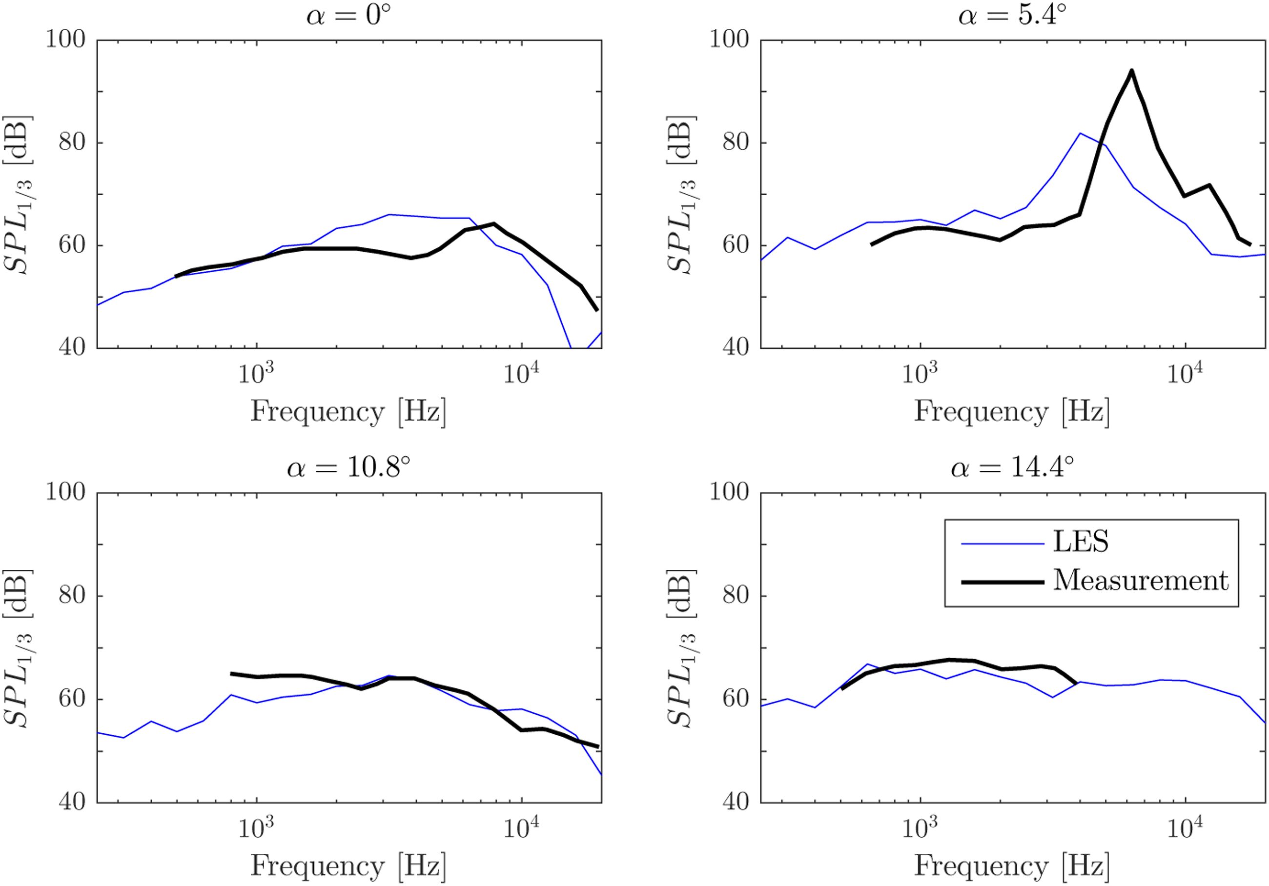

Vertical axis wind turbines blade

The validation is made for the aerodynamics of the VAWT model. The measurement data by Li et al.²⁵ are referred, who experimentally examined the effect of solidity on aerodynamic forces of the VAWT with the different number of blades. The six-component balance equipped on the bottom of the rotor shaft was used to quantify the force and moment in their experiment. The measured results obtained for the three-bladed rotor with the tip speed ratio of 1.78 are used here. The free stream velocity is 8.0 m/s, and the rotor diameter is 2.0 m. Figure 8 shows the simulated and measured torque coefficient C_T, which is defined as $C_{T} = T / 0.5 ρ A R U_{\infty}^{2}$ where T is the torque produced by one blade. It can be observed that the curves agree well in the upwind side, but large discrepancies arise in the downwind side. This difference is caused probably because the support structures are ignored in the simulation. The wake generated from the support structure interacts with the blade surface downwind, which can be considered to reduce the blade performance. Another reason can be due to the drag loss by the support structures that decrease the total rotor torque, which are not modeled in the simulation.

Figure 8.

Comparison for the torque coefficient of a single blade during one revolution between the measurement by Li et al.²⁵ and the present model.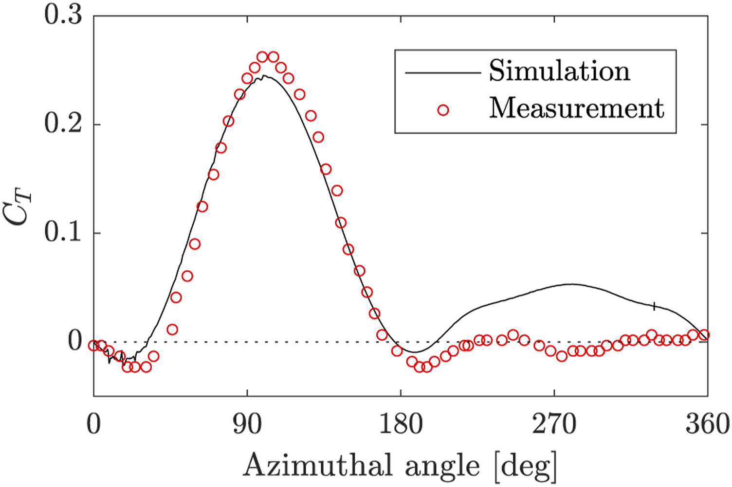

Results and discussion

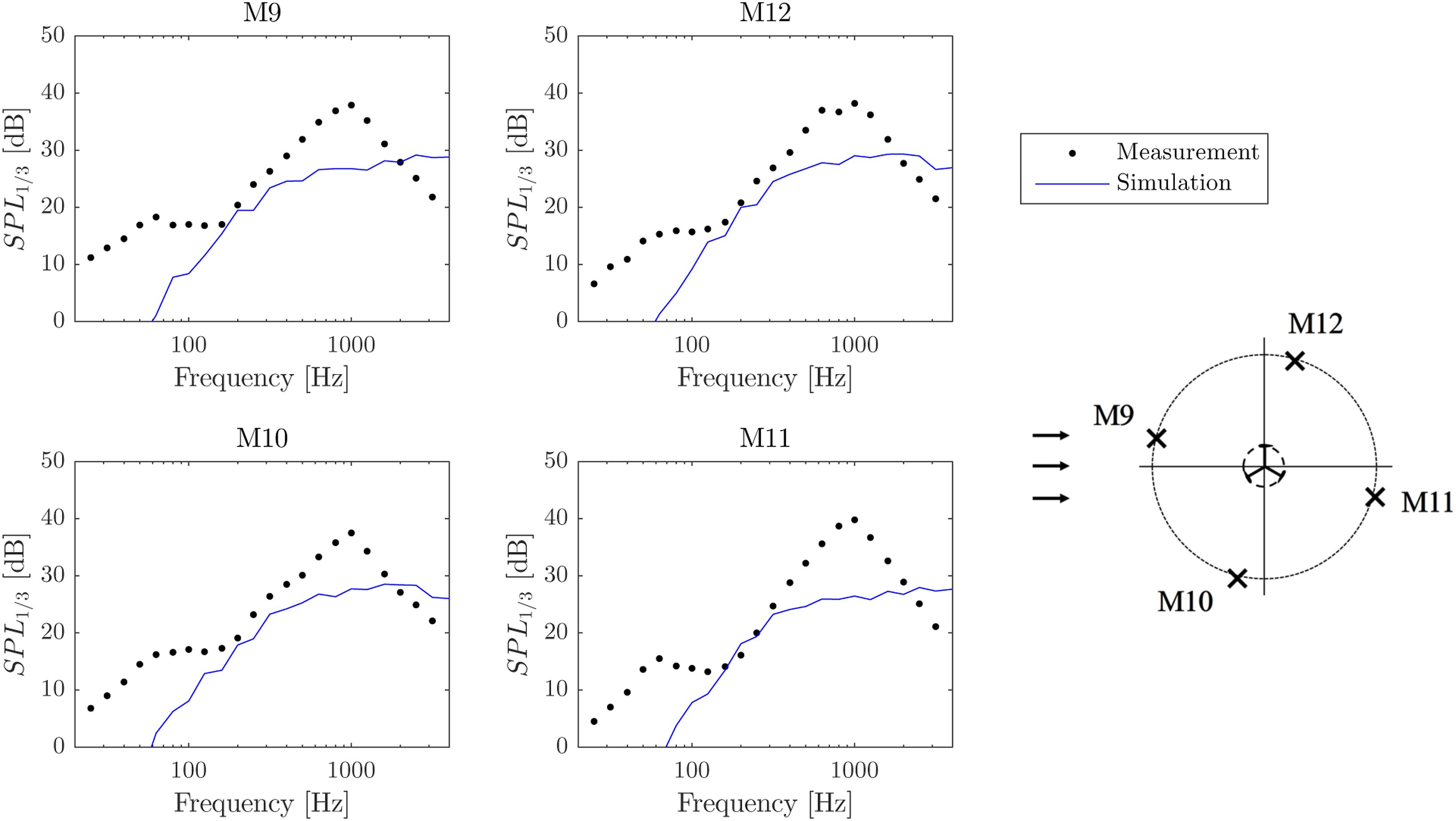
The noise of the VAWT is predicted and the SPL is validated by comparing with measurement data. Figure 9 and Figure 10 show the A-weighted one-third octave band spectra of the SPL with reference p_ref observed at radial distances of 1.4D and 2.8D for eight and four different directions, respectively. The measured SPL at frequencies up to 100 Hz can be considered to originate from the noise of the traffic road.

Figure 9.

1/3 octave band spectra of the measured and predicted sound pressure level observed at radial distance of 1.4D from the center of rotation with reference p_ref = 2 × 10⁻⁵ Pa.

Figure 10.

1/3 octave band spectra of the measured and predicted sound pressure level observed at radial distance of 2.8D from the center of rotation with reference p_ref = 2 × 10⁻⁵ Pa.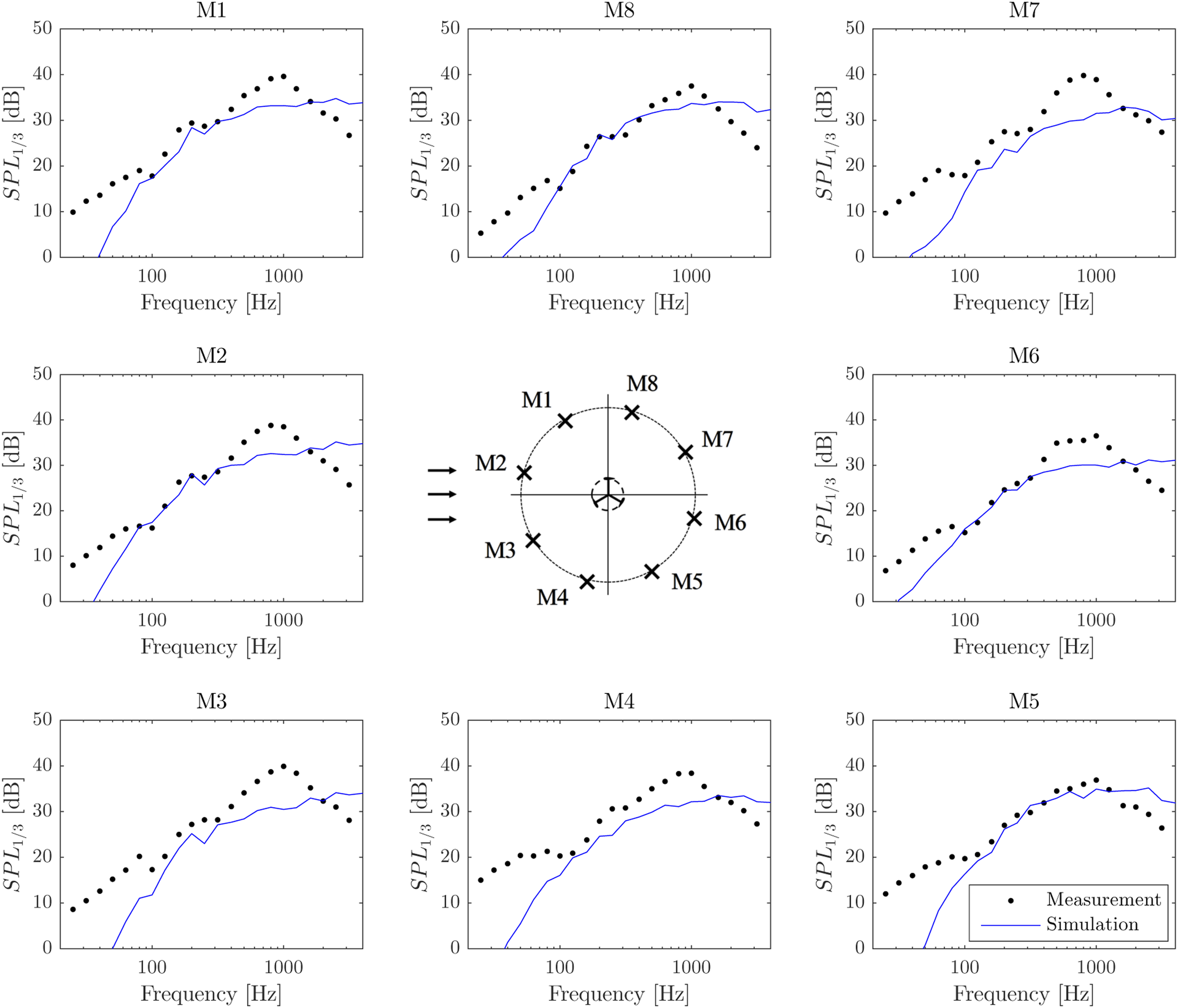

The measured spectra have broadband characteristics centered at around 630 or 800 Hz, and the prediction is able to reproduce the increase of the SPL to the peak. The maximum SPL in Figure 9 is generally underestimated by a few decibels except for those at the locations of M3 and M7 which have differences by almost 10 dB. The possible reason for these large discrepancies is that the model does not simulate the actual wind condition. The wind speed was varying unsteadily during the recording period as shown in Figure 4, so the tip speed ratio could intermittently become quite low assuming that the rotational speed was almost constant. While the simulation predicts an attached flow around the blade surface due to high tip speed ratio, the blade could be becoming stalled and generating the separation stall noise when the sound was recorded at these locations.

It is also noted that small peaks can be seen in the measured spectra for distance of 1.4D at around 200 Hz at all recorded locations. This tonal peak is probably caused by the struts, which will be discussed later.

The discrepancies of the sound pressure around the peak become even larger at distance of 2.8D than at distance of 1.4D, and these differences can be considered to be caused by neglecting the ground effect. The observer receives both the direct sound wave and the wave reflected on the ground, but only the direct sound is considered in the simulation. The ground effect is expected to be more significant at greater distance, and if this is the case, care has to be taken when the noise received at long distance is to be predicted. Generally, the observed sound is increased at low frequencies and is attenuated at high frequencies due to the ground reflection. This might explain the overprediction seen at frequencies higher than around 2000 Hz for the spectra in both Figures 9 and 10.

Figure 11 shows the directivity of the predicted and measured overall SPL at radial distances of 1.4D and 2.8D. They are calculated by summing the SPL of the frequency bands from 25 to 3100 Hz. Note that the agreement of the overall SPL does not necessarily mean that the predicted overall SPL is accurate because the SPL shown in Figures 9 and 10 are under- and over-predicted in the low and high frequency range, respectively, and they can be cancelled out by summation. There is little dependence of directivity in the measurements, while the prediction indicates stronger directivity. The overall SPL is predicted to be higher in the upwind than in the downwind side for both radial distance cases.

Figure 11.

Directivity of the predicted and measured overall SPL at radial distances of 1.4D (left) and 2.8D (right).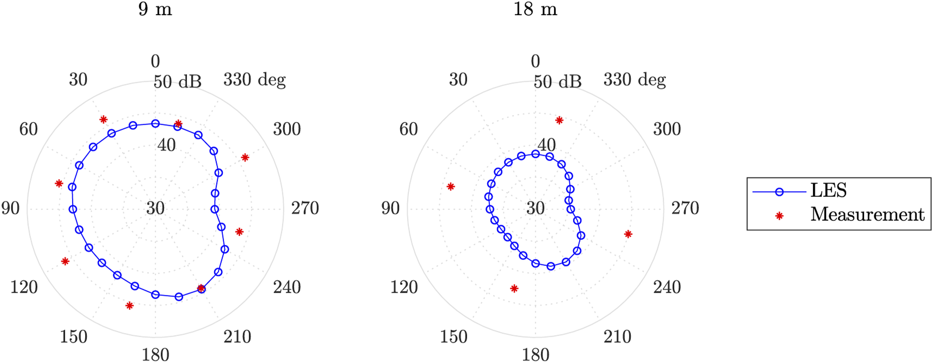

The decay of the predicted overall SPL by doubling the distance is consistent with the theoretical values for the attenuation of the sound by the distance from the sound source. The decay presented in Figure 11 for each of the 24 observation directions falls within the range between 3.7 and 5.9 dB. These numbers are less than the theoretical decay for spherical spreading per doubling of distance that is 6 dB but larger than the decay for cylindrical spreading that is 3 dB.

The sound emitted from the blade is more dominated in the total noise than the sound from the struts. Figure 12 shows the overall SPL calculated using the sound source from only a single blade, only struts, and both of them. The presented values are the sound observed at radial distances of 1.4D for different azimuth angles. They are calculated by summing the SPL of all the audible frequency bands from 20 to 20,000 Hz. It is obvious that the overall SPL from the blade is much larger than the SPL from struts at all azimuth directions.

Figure 12.

Overall SPL calculated using the sound source from only a single blade, only struts, and both of them for observation locations around different azimuthal directions at radial distances of 1.4D.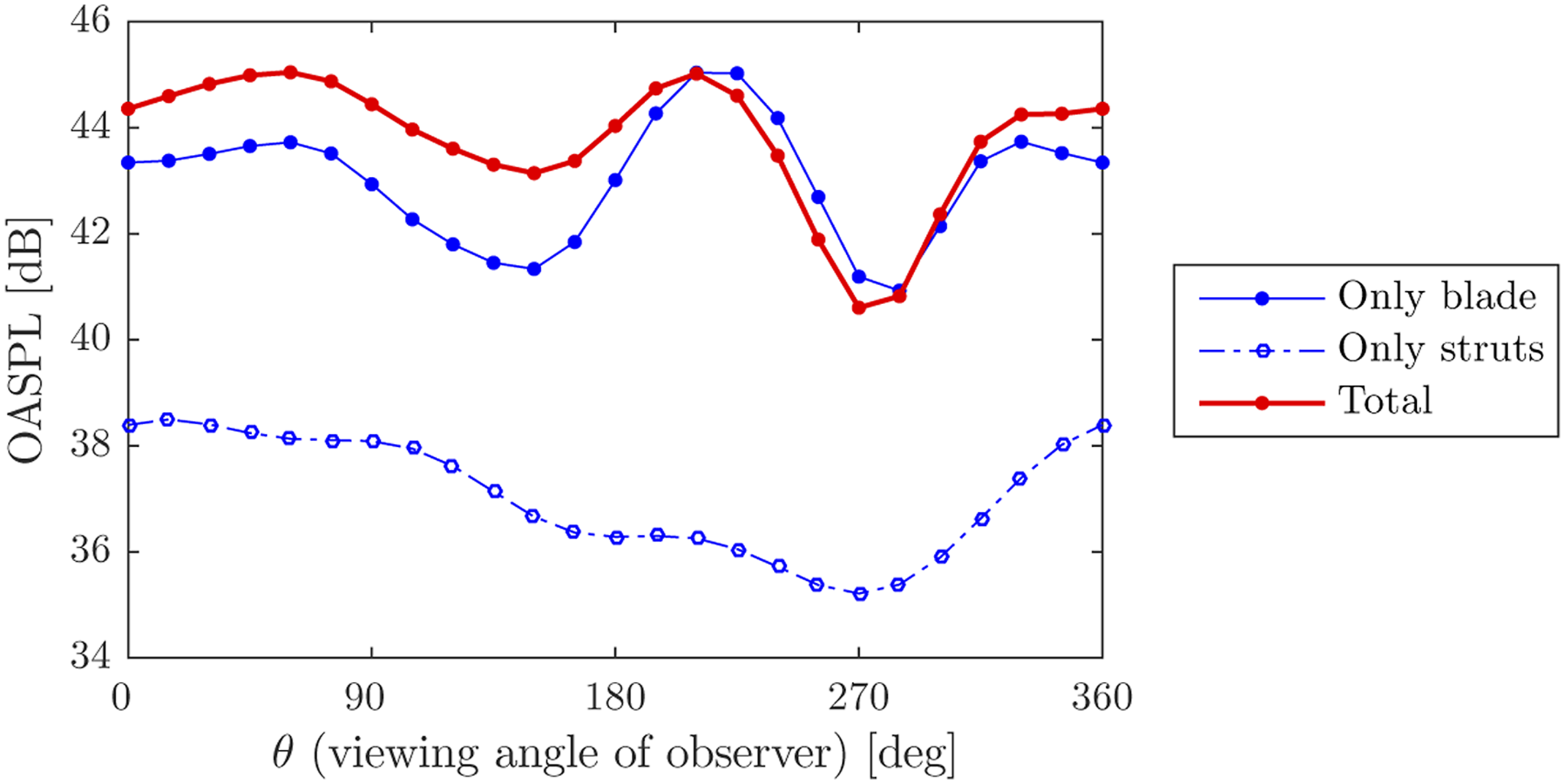

The first term in the loading noise expressed by equation (5) includes the variable of the time derivative of pressure, and the time history of this term $p_{L 1}^{'}$ during one revolution is shown in the left plot in Figure 13. The spectra of the SPL attributed to three and two terms of each integral in the loading and thickness noise represented in Equation (5) and Equation (4), denoted by $p_{L 1}^{'}$ , $p_{L 2}^{'}$ , $p_{L 3}^{'}$ , $p_{T 1}^{'}$ , and $p_{T 2}^{'}$ , are shown in the right plot in Figure 13. The presented data correspond to the sound pressure observed at θ = 90° at distance 1.4D radiated only from a single blade and two struts.

Figure 13.

Time history of the term related to the pressure derivative in the sound pressure of the loading noise during one revolution (left) and spectra of the SPL for each term in the loading and thickness noise (right). The data presented are the sound pressure observed at θ = 90° at distance 1.4D radiated from a single blade and two struts.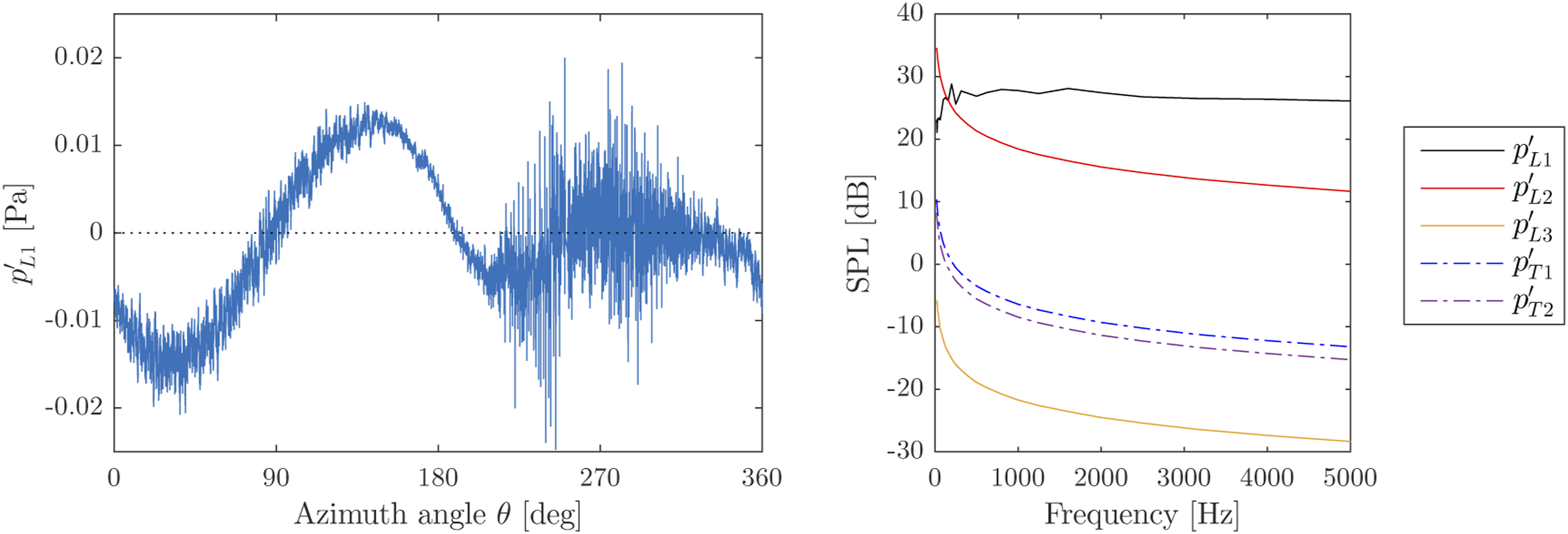

It can be seen from the left plot that $p_{L 1}^{'}$ fluctuates more when the blade travels in the downwind than in the upwind side. The amplitude of fluctuations becomes small when the blade moves around θ = 0° and 180°. The right plot indicates that the first two terms of the loading noise are more dominant than the terms of the thickness noise, and especially the contribution of the term $p_{L 1}^{'}$ is highest in almost all frequency range among all terms. The loading noise is involved with the aerodynamic flow, while the thickness noise is determined by the movement of the object. Some works^5,7,23 studying for VAWTs which have a diameter of one order smaller than ours state that the thickness noise is the main noise source and the sound pressure is dominated by the blade passing frequency. On the contrary, the loading noise plays a more important role for the VAWT of this study, as the rotational frequency is much lower and may be less relevant to the magnitude of the total noise level.

A periodic swishing sound was clearly heard during the measurement, and the turbine apparently emits the loud sound when the blade passes at a certain azimuth location during revolution. In order to estimate the azimuth position where the sound is strongly generated, the instantaneous overall SPL during revolution is calculated as shown in Figure 14. The presented data correspond to the sound radiated from a single blade and two struts observed at radial distance of 1.4D from four different azimuth angles, θ = 0°, 90°, 180°, and 270°. In the calculation, the data series of the sound pressure during the time period for the blade to rotate by 30° is extracted, and they are filtered to obtain the spectrum after the hanning window is applied. Then, the overall SPL is obtained by summing up the SPL in all bands.

Figure 14.

Instantaneous overall SPL during revolution observed from four different azimuth angles, θ = 0°, 90°, 180°, and 270° at radial distance of 1.4D.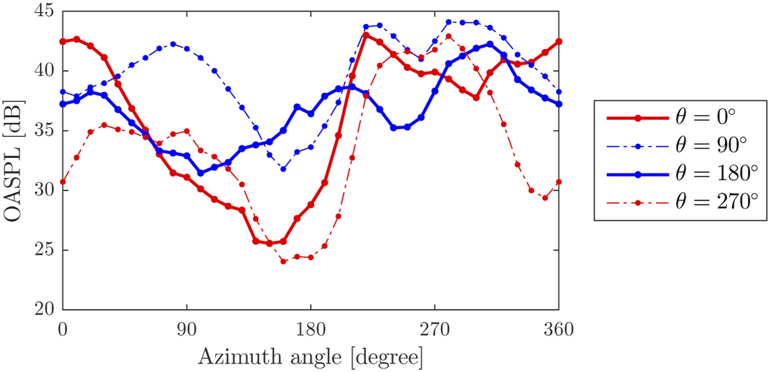

The received sound is likely to be louder when the blade passes in the downwind than in the upwind side, although the observer at θ = 90° is positioned closest when the blade passes at that azimuth angle and thus the overall SPL received there is relatively large. This is consistent to the fact found by Pearson⁷ that the dominant source is generated in the downstream half at high tip speed ratio. It can be considered that the blades moving in the downwind suffer from the wake created in the upwind and the interaction of the wake contributes to generate strong sound sources.

Figure 15 shows the time derivative of pressure $\dot{p}$ on the surface seen from the outside and inside of the rotor when the blade and struts are located at several different azimuth angles. It indicates that intensive fluctuation of $\dot{p}$ is concentrated around the trailing edge at all azimuth angles presented. Small fluctuations can be seen over a large area of the surface on the suction side of the blade, and the fluctuations are present on the pressure side in the area close to the trailing edge as well. It can be assumed that these small fluctuations on the surface attribute to the source of the turbulent boundary layer trailing edge noise. While the pressure fluctuates randomly on the blade surface, Figure 15 also indicates that the wavy pattern occurs on the strut surface.

Figure 15.

Time derivative of surface pressure seen from the outside (left) and inside (right) of the rotor.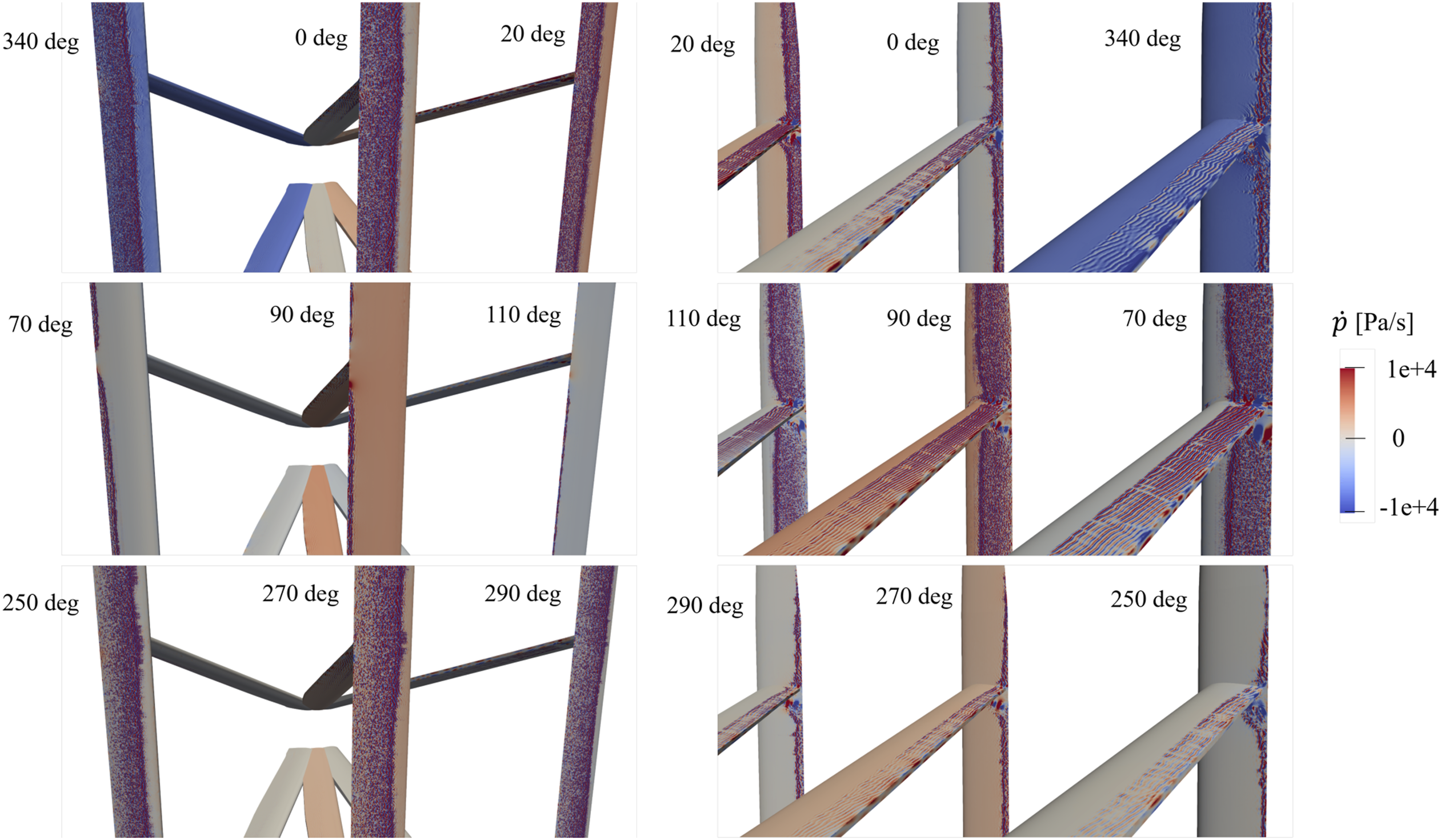

The inflow turbulence noise is not properly predicted in the simulation but it could be another important sound source. Eddies from the atmospheric turbulence which approach the leading edge are distorted and radiated sound which in turn is scattered at the leading and trailing edge.³⁷ However, no significant pressure fluctuation can be observed at the leading edge in Figure 15. One of the reasons why the SPL presented in Figure 9 and Figure 10 is underpredicted could be that the simulation does not include turbulence in the freestream wind.

It can be considered that the second peak at around 200 Hz seen in the measured spectra in Figure 9 is caused by the sound source from the strut surface. Figure 16 shows the spectra of the SPL observed at location of M2 which are calculated using the sound source from only the blades, only the struts, and both of them. In Figure 16, the peak at 200 Hz does not appear when the sound source from the struts is not included but is highly dominant in the spectrum when considered.

Figure 16.

1/3 octave band spectra of the SPL observed at location M2 calculated radiated from only the blades, only the struts, and both of them.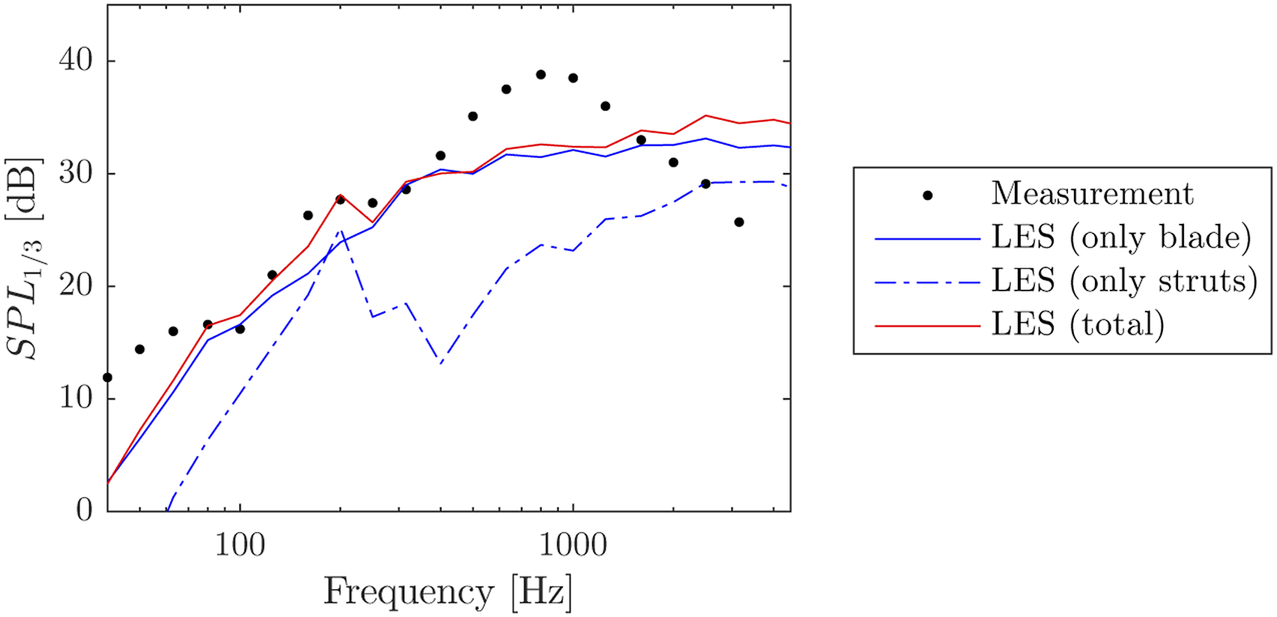

Figure 17 shows the vortex structure around the strut located at θ = 270°. To visualize the vortex formation, the Q-criterion is used, which calculates the second invariant of the velocity gradient tensor expressed as Q = 0.5 (Ω_ijΩ_ij−S_ijS_ij) where Ω_ij = 0.5 (∂u_i/∂x_j−∂u_j/∂x_i) is the vorticity tensor and S_ij = 0.5 (∂u_i/∂x_j + ∂u_j/∂x_i) is the rate-of-strain tensor. The left picture in Figure 17 represents the iso contour for Q = 60 s⁻² around the trailing edge, and the right picture represents the contour plot for the plane sliced perpendicular to the strut span at 93% of rotor radius. The vortices appear around the middle of the chord. They are convected maintaining the wave-shaped structure and are then released while interacting with the blunt trailing edge. The vortex shedding cannot be recognized in the wake of the blade at all, as seen in the left picture. The local flow condition around the struts is different from that of the blades, as the tip speed ratio of the struts is low. These flow characteristics around the struts can be considered to generate the tonal noise observed at 200 Hz in Figure 16.

Figure 17.

Iso contour around the upper strut located at θ = 270°. Contour for Q = 60 s⁻² around the trailing edge (left) and contour plot for the plane sliced perpendicular to the strut span at 93% of rotor radius (right).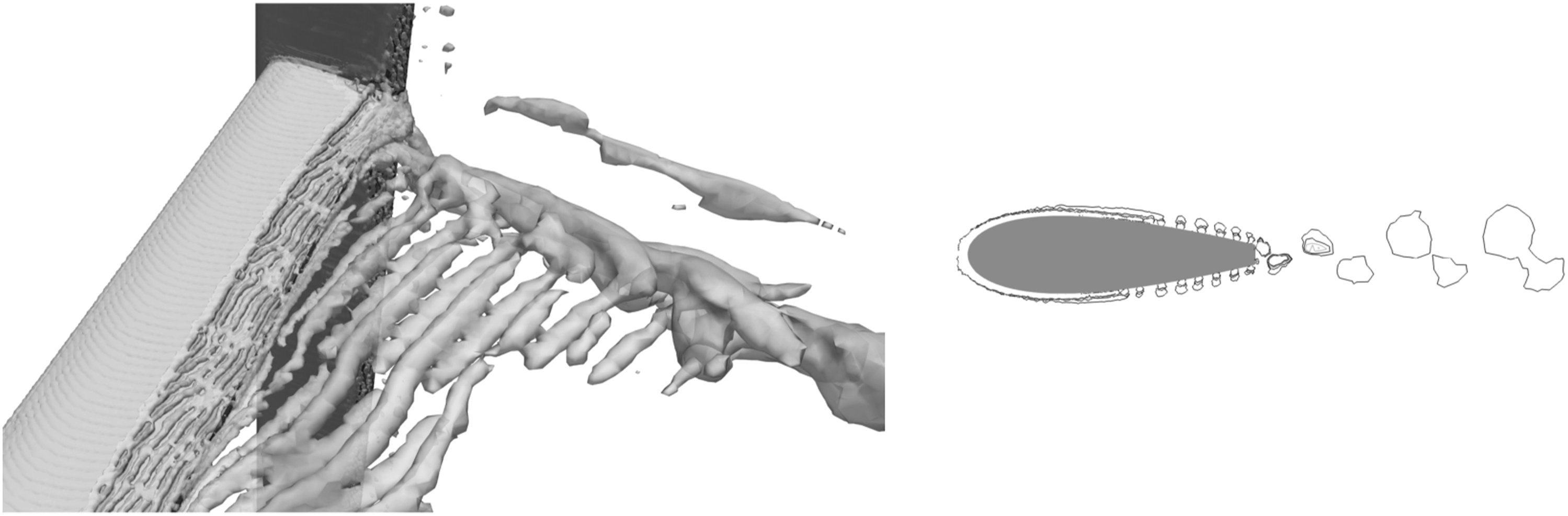

Conclusion

This study investigates the numerical method of noise prediction for a 12 kW VAWT using LES and the FW-H acoustic analogy. The sound pressure levels predicted for high tip speed ratios are compared with measurements. The measured spectra have broadband characteristics centered at around 800 Hz, and the simulation is able to capture the increase of the sound pressure level up to 1000 Hz for the spectra observed at the radial distance of 1.4 rotor diameter with differences of a few dB. However, the numerical model significantly underpredicts the noise observed at 2.8 rotor diameter distances. This discrepancy could be caused by neglecting the effect of the ground reflection in the simulation. While the thickness noise is considered to be predominant for small-scaled VAWTs, the simulation results reveal that the loading noise is the dominant sound source for this turbine. The time history of the predicted sound pressure during revolution shows large fluctuations especially when the blade travels in the downwind side. One of the causes for these fluctuations can be the interaction between the blades in the downwind and the wake created in the upwind. Although the blade is a main contributor to the total noise, it is also found that the struts emit small tonal noise at around 200 Hz which are caused by vortices generated from the strut surface around the middle of the chord and blunt trailing edge. The atmospheric turbulence is not considered in the simulation, but it could be a significant contribution to the total noise. It will be further investigated to examine whether this effect is important for this turbine in order to improve the accuracy of the prediction. Also, it should be examined to simulate under a wide range of tip speed ratios, as the sound source will differ when dynamic stall occurs at low tip speed ratio from what was observed in this study case.

Footnotes

Declaration of conflicting interests

The authors declared no potential conflicts of interest with respect to the research, authorship, and/or publication of this article.

Funding

The authors disclosed receipt of the following financial support for the research, authorship, and/or publication of this article: This work was conducted within the ST and UP for Energy strategic research framework and is part of ST and UP for Wind. The computations were enabled by resources provided by the Swedish National Infrastructure for Computing (SNIC) at NSC at Linköping University partially funded by the Swedish Research Council through grant agreement no. 2020/5-321.

ORCID iDs

Aya Aihara

Karl Bolin

References

Pedersen

van den Berg

Bakker

, et al. Response to noise from modern wind farms in the Netherlands. J Acoust Soc Am 2009; 126(2): 634–643.

Michaud

Feder

Keith

, et al. Exposure to wind turbine noise: Perceptual responses and reported health effects. J Acoust Soc Am 2016; 139(3): 1443–1454.

Wagner

Bareiss

Guidati

. Wind Turbine Noise. Environmental Engineering. New York, NY: Springer, 1996.

Eriksson

Bernhoff

Leijon

. Evaluation of different turbine concepts for wind power. Renew Sustain Energ Rev 2008; 12(5): 1419–1434.

Weber

Becker

Scheit

, et al. Aeroacoustics of Darrieus wind turbine. Int J Aeroacoustics 2015; 14(5–6): 883–902.

Brooks

Pope

Marcolini

. Airfoil Self-Noise and Prediction. Technical Report 1218. NASA, 1989.

Pearson

. Vertical axis wind turbine acoustics. PhD Thesis. Cambridge, UK: University of Cambridge, 2014.

Ottermo

Möllerström

Nordborg

, et al. Location of aerodynamic noise sources from a 200 kW vertical-axis wind turbine. J Sound Vib 2017; 400: 154–166.

Möllerström

Ottermo

Hylander

, et al. Noise emission of a 200 kw vertical axis wind turbine. Energies 2016; 9(1): 19.

10.

Göçmen

Özerdem

. Airfoil optimization for noise emission problem and aerodynamic performance criterion on small scale wind turbines. Energy 2012; 46(1): 62–71.

11.

Bertagnolio

Madsen

Fischer

. A combined aeroelastic-aeroacoustic model for wind turbine noise: Verification and analysis of field measurements. Wind Energ 2017; 20(8): 1331–1348.

12.

Kaviani

Nejat

. Aerodynamic noise prediction of a MW-class HAWT using shear wind profile. J Wind Eng Ind Aerodynamics 2017; 168: 164–176.

13.

Moriarty

Migliore

. Semi-empirical Aeroacoustic Noise Prediction Code for Wind Turbines. Technical report. Golden, Colorado: National Renewable Energy Laboratory, 2003.

14.

Zhu

Heilskov

Shen

, et al. Modeling of aerodynamically generated noise from wind turbines. J Solar Energ Eng 2005; 127(4): 517–528.

15.

Leloudas

Zhu

Sørensen

, et al. Prediction and reduction of noise from a 2.3 MW wind turbine. J Phy: Conf Series; 75: 12–83.

16.

Rasam

Botha

Bolin

, et al. Aerodynamic noise prediction for a wind turbine using numerical flow simulations and semi-empirical modelling approaches. In: 22nd AIAA/CEAS Aeroacoustics Conference, Lyon, France, 30 May 2016.

17.

Botha

Rasam

Catháin

, et al. Some noise predictions for small wind turbines. In: Proceedings of ISMA 2016—International Conference on Noise and Vibration Engineering and USD2016 - International Conference on Uncertainty in Structural Dynamics, KU Leuven, Departement Werktuigkunde, pp. 4019–4032.

18.

Botha

Shahroki

Rice

. An implementation of an aeroacoustic prediction model for broadband noise from a vertical axis wind turbine using a CFD informed methodology. J Sound Vib 2017; 410: 389–415.

19.

Sucameli

. Development and Implementation of an Aeroacoustic Module for Wind Turbine Noise Prediction. Master’s Thesis. Milan, Italy: Politecnico di Milano, 2017.

20.

Mohamed

. Aero-acoustics noise evaluation of H-rotor Darrieus wind turbines. Energy 2014; 65: 596–604.

21.

Wasala

Storey

Norris

, et al. Aeroacoustic noise prediction for wind turbines using large eddy simulation. J Wind Eng Ind Aerodyn 2015; 145: 17–29.

22.

Tadamasa

Zangeneh

. Numerical prediction of wind turbine noise. Renew Energ 2011; 36(7): 1902–1912.

23.

Ghasemian

Nejat

. Aero-acoustics prediction of a vertical axis wind turbine using Large Eddy Simulation and acoustic analogy. Energy 2015; 88: 711–717.

24.

Yen

Ahmed

. Enhancing vertical axis wind turbine by dynamic stall control using synthetic jets. J Wind Eng Ind Aerodyn 2013; 114: 12–17.

25.

Maeda

Kamada

Murata

, et al. Wind tunnel and numerical study of a straight-bladed vertical axis wind turbine in three-dimensional analysis (Part I: For predicting aerodynamic loads and performance). Energy 2016; 106: 443–452.

26.

Williams

Hawkings

. Sound generation by turbulence and surfaces in arbitrary motion. Philos Trans R Soc Lond A 1969; 264(1151): 321–342.

27.

Lighthill

. On sound generated aerodynamically I. general theory. Proc R Soc Lond Ser A 1952; 211(1107): 564–587.

28.

Lighthill

. On sound generated aerodynamically II. turbulence as a source of sound. Proc R Soc Lond Ser A 1954; 222(1148): 1–32.

29.

Farassat

. Derivation of Formulations 1 and 1A of Farassat. Technical Report NASA/TM-2007-214853. NASA Langley Research Center Hampton, 2007.

30.

Lerner

Boldes

. Applied Aerodynamics. Norderstedt, Germany: BoD–Books on Demand, 2012.

31.

Goude

Rossander

. Force measurements on a VAWT blade in parked conditions. Energies 2017; 10(12): 1954.

32.

Weller

Tabor

Jasak

, et al. A tensorial approach to computational continuum mechanics using object-oriented techniques. Comput Phy 1998; 12(6): 620–631.

33.

Nicoud

Ducros

. Subgrid-scale stress modelling based on the square of the velocity gradient tensor. Flow, Turbulence and Combustion 1999; 62(3): 183–200.

34.

Weickert

Teike

Schmidt

, et al. Investigation of the LES WALE turbulence model within the lattice boltzmann framework. Comput Math Appl 2010; 59(7): 2200–2214.

35.

Rezaeiha

Kalkman

Blocken

. CFD simulation of a vertical axis wind turbine operating at a moderate tip speed ratio: Guidelines for minimum domain size and azimuthal increment. Renew Energ 2017; 107: 373–385.

36.

Paterson

Vogt

Fink

, et al. Vortex noise of isolated airfoils. J Aircraft 1973; 10(5): 296–302.

37.

Ainslie

Scott

. Theoretical modelling of noise generated by wind turbines. Wind Eng 1990; 14: 9–14.

Aeroacoustic noise prediction of a vertical axis wind turbine using large eddy simulation

Abstract

Keywords

Introduction

Acoustic calculation

Turbine geometry

Acoustic measurement

Numerical approach

Validation of numerical model

Static single blade

Vertical axis wind turbines blade

Results and discussion

Conclusion

Footnotes

Declaration of conflicting interests

Funding

ORCID iDs

References