
Abstract
This paper presents the contribution from the German Aerospace Center (DLR) to the first liner benchmark challenge under the framework of the International Forum for Aviation Research (IFAR). Therefore, two sets of acoustically damping wall treatments, called ‘liner samples’, have been produced by additive manufacturing based on the design data provided by NASA coordinating this benchmark. These liner samples have been integrated and acoustically characterized in the liner flow test facility DUCT-R at DLR Berlin as well as in the liner flow test facility GFIT at NASA Langley. Besides the dissipation coefficients and the axial pressure profiles, the liner wall impedance was educed by first determining the axial wave numbers and then applying a straightforward method based on the one-dimensional Convected Helmholtz Equation. Finally, the comparison of the liner impedance values to the NASA results show a fairly good agreement.
Introduction
Liners as a wall treatment for acoustic damping are one of the most important technologies for aircraft noise reduction. They are usually integrated in the inlet and bypass duct of aero-engines in order to reduce the engine noise emission propagating from various internal sources. Although there exist fairly mature technology solutions for liner design, the predictive capabilities of liner performance under real application conditions are still unsatisfactory. There remains the need for experimental testing of liner samples in purpose-built liner flow duct facilities. This yields the challenge to ensure comparability between the different liner test facilities existing worldwide and the correspondingly applied post-processing methods and prediction approaches.
To address this challenge, the International Forum for Aviation Research (IFAR) initiated a benchmark activity devoted to compare acoustic liner testing and performance prediction. The DLR Department of Engine Acoustics took part in this liner benchmark managed by NASA. The liner benchmark is divided into three different challenges: Challenge #1: Comparison of Liner Test Facilities Challenge #2: Propagation Code Comparison Challenge #3: Impedance Eduction Comparison
This paper will mainly focus on the DLR contribution to Challenge #1 and a corresponding comparison to NASA results. For Challenge #1, NASA provided CAD drawings of selected generic liner designs to all participating partners within IFAR. Two liner configurations are considered for this challenge. The first is a uniform liner, for which the impedance should be nearly constant over the length of the liner. The second is a two-segment liner, where the only difference between the two axial segments is the depth of the liner cavity. Measurement results from these liner configurations have been published by NASA in Jones et al.1,2
The goal of Challenge #1 is to gather data from multiple test rigs with the same liner configurations manufactured using 3D printing. By sharing the data with each participant, it will be possible to evaluate dependence of these results on fabrication, data acquisition and analysis (e.g., impedance eduction) approaches. Within this paper the DLR contribution to Challenge #1 and the comparison of the DLR results with NASA data will be presented.
IFAR challenge #1 liner geometries
The two liner configurations of IFAR Challenge #1 are shown in Figure 1. The first, homogeneous liner sample
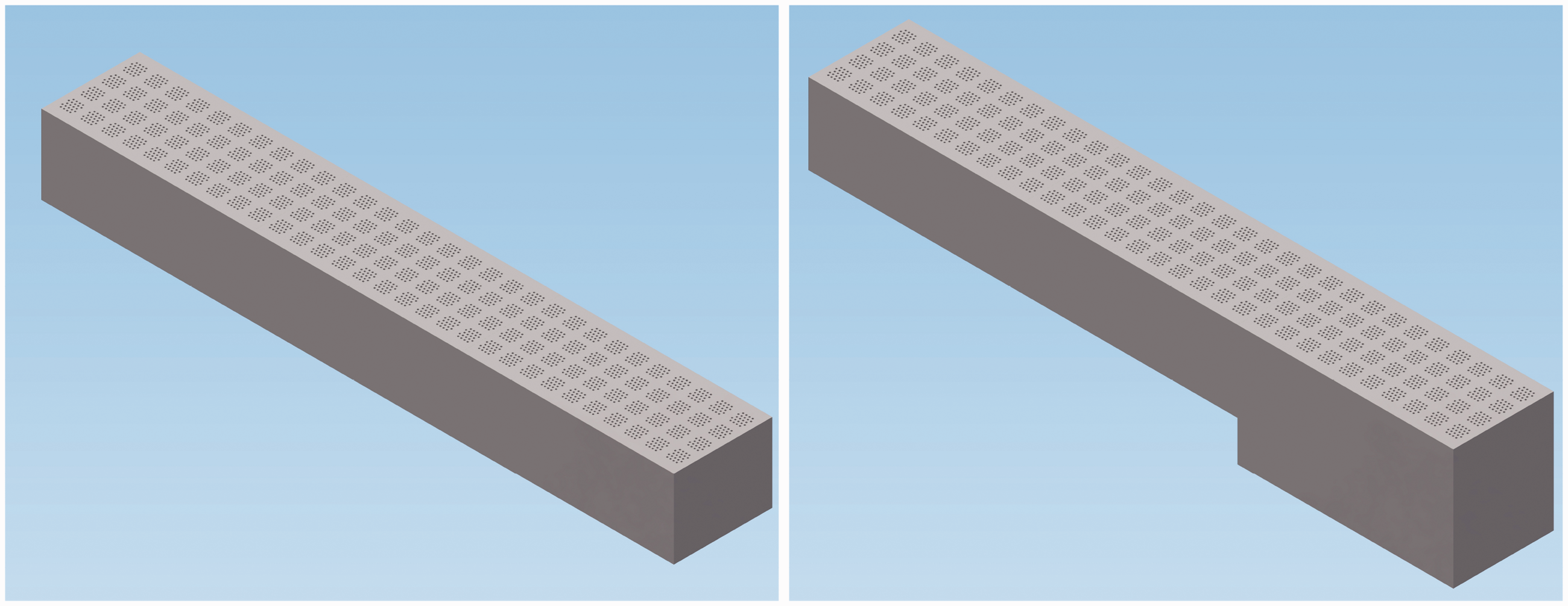
CAD models of the liner samples (left: constant depth liner
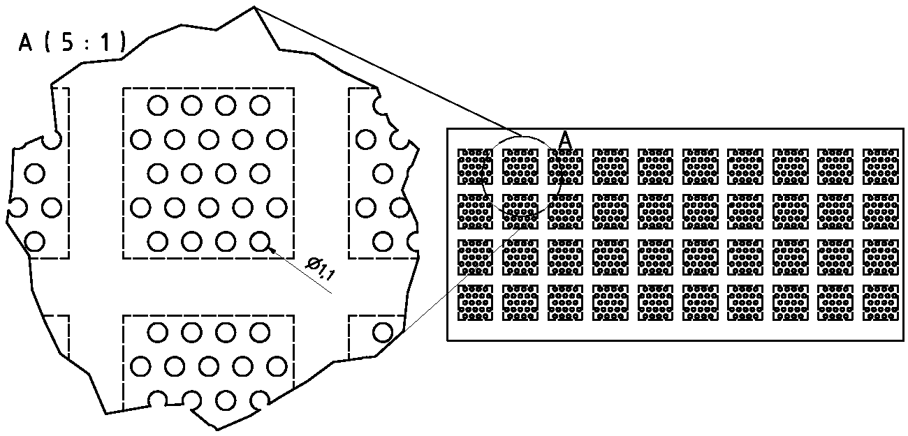
Detailed sketch of the liner facesheet geometry.
NASA GFIT facility and NASA impedance eduction method
The NASA Langley Grazing Flow Impedance Tube (GFIT, see Figure 3) has a 50.8 mm-wide (
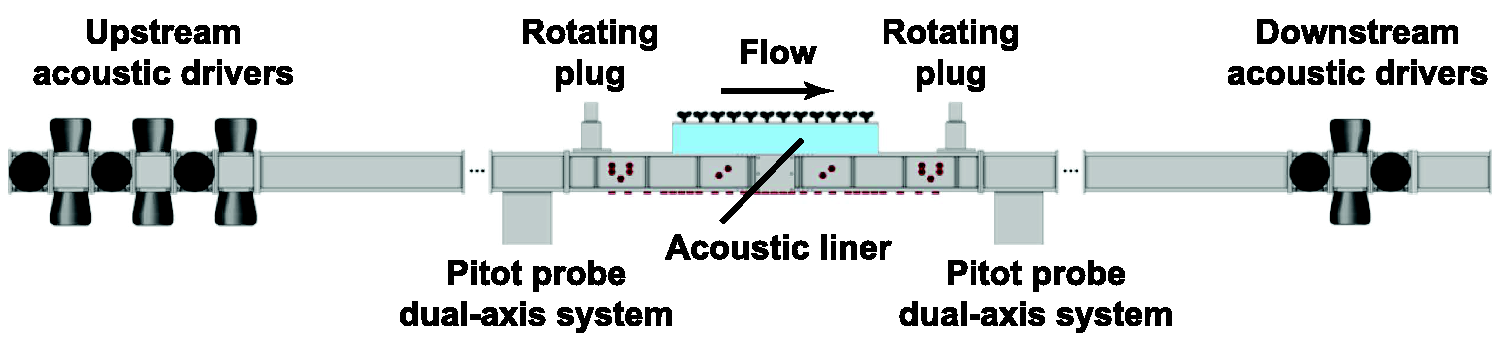
Sketch of the NASA Grazing Flow Impedance Tube (GFIT). Microphones depicted as small cylinders, placed on all walls surrounding the acoustic liner section.
The impedance of the constant depth liner (
For the two-segment liner (

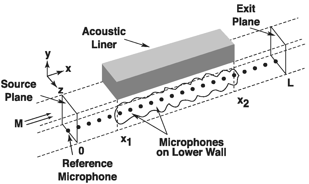
Sketch of computational domain in GFIT.
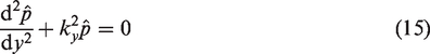
The local-reacting wall boundary condition presented by Myers
3
is given by


If the acoustic impedance of the liner is known, equations (1) to (4) may be solved via a finite element method to determine the acoustic pressure field throughout the GFIT. Instead, the CHE method employs an optimizer to search for an impedance where the acoustic pressures predicted via this finite element method match the corresponding acoustic pressures measured with the microphones along the lower wall of the GFIT to within an acceptable tolerance. This impedance is taken to be the impedance of the liner.
DLR DUCT test rig and liner manufacturing
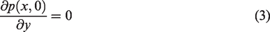
The DLR liner test facility DUCT-R consists of a flow duct with a cross-section of 60 mm (W) by 80 mm (H). Driven by an upstream radial compressor a mean flow Mach number on the centerline of up to 0.3 can be set. The duct itself is setup symmetrically with loudspeakers (A and B) at the upstream and downstream ends, two (hard-wall) measurement sections and a liner mounting module (face-to-face section) in the center as shown in the schematic sketch in Figure 5.
Sketch of the DLR liner test facility DUCT-R with the two measurement (hard-wall) sections and the liner mounting module in between.
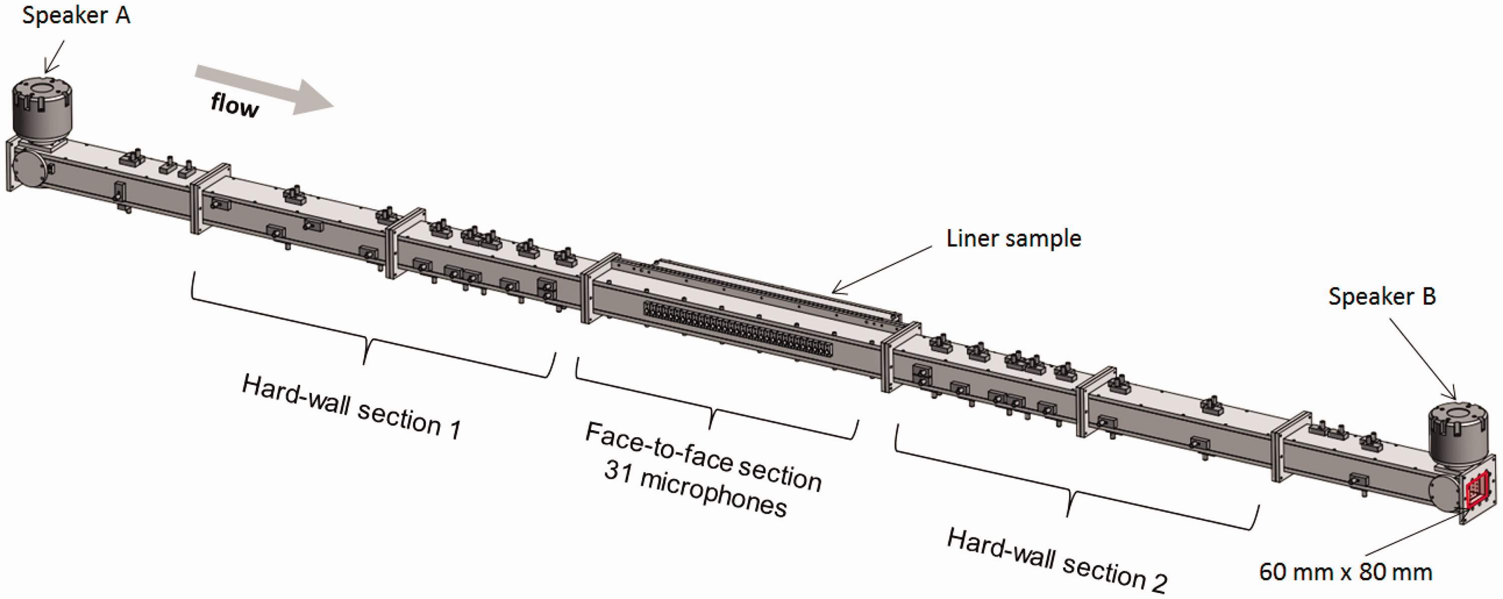
Microphones are installed at different axial positions in both the hard wall measurement sections as well as face-to-face in the liner module. The face-to-face microphones are flush-mounted in the wall on the opposite side of the liner surface. Figure 6 shows a photo of the DUCT-R setup applied for this investigation. Further details about the test rig and the acoustic measurements system can also be found in Busse-Gerstengarbe et al. 4 and in Schulz et al. 5 The variety of microphone positions enables the evaluation of the scattering coefficients (reflection, transmission and dissipation) of the liner module via the hard-wall measurement sections and the acquisition of the sound field directly in the lined duct section via the face-to-face microphones. From both data sets, determination of the liner impedance is possible using various eduction methods. This includes modal and nonmodal based impedance eduction approaches as described in Weng et al. 6 The acoustic excitation was accomplished using single tones with an incident sound wave amplitude of approximately 140 dB.
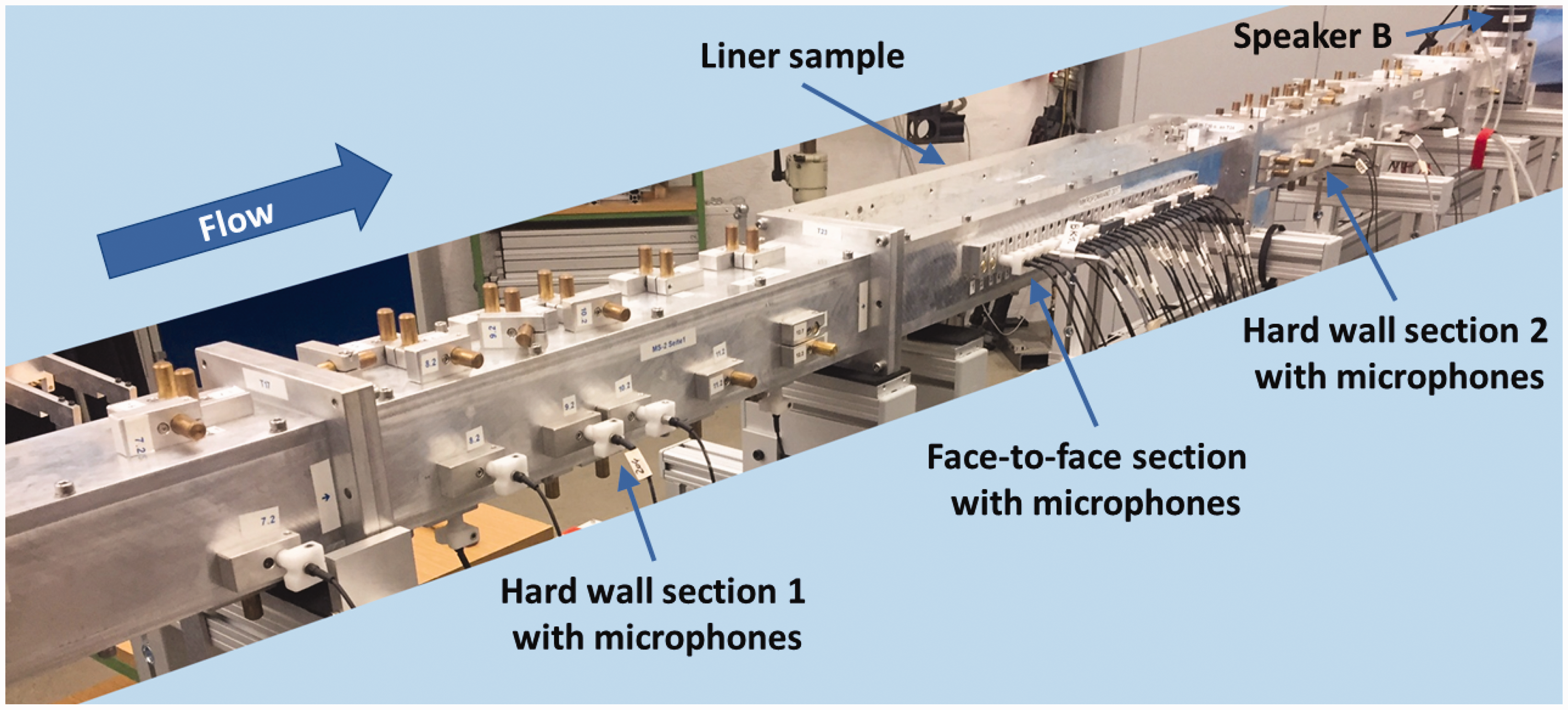
Photo of the DLR liner test facility DUCT-R with the liner mounting module in the center.
The provided CAD was modified to increase the thickness of the outer axial partitions to 6.3 mm in order to fit into the liner mounting device of the DLR liner test facility DUCT-R. However, this adaptation does not change the geometric configuration of the active liner surface as part of the duct wall. The liner samples were fabricated using the 3D-printing stereolithography process with indurating liquid photopolymer resin. Since the length of the liner samples exceeds the maximum printable size of our device, the samples were printed in three segments consisting each of 4-by-10 cavities. A 3.8 mm thick aluminum plate was used as a backplate.
A major challenge during manufacturing was to find the best-suited printing configuration for an optimal printing accuracy across the entire spatial range since the size of the liner segments corresponds to almost the maximum permissible printing size of the printer device. For this purpose, a number of test prints with varying print parameters were conducted. In addition, to further increase manufacturing accuracy, all samples were designed with a 1 mm oversize. During post processing the samples were sanded and the oversize was milled to match the nominal specifications. Subsequently, the segments were evaluated yielding maximum deviations of about 0.05 mm compared to the required specifications. The perforation diameters vary between 1.07 mm and 1.12 mm. The left photo in Figure 7 shows a single liner segment after post processing and the right photo shows the homogeneous liner sample installed in the DUCT-R.
Photos of the 3D printed post processed liners (left: single liner segment; right: liner sample installed in the duct).
DLR data post processing, results and discussion
This section presents the DLR data analysis steps and the corresponding results from the liner samples
Scattering coefficients
The damping performance of the liner is evaluated using the dissipation coefficient. This is an integral value of the acoustic power that is absorbed while a sound wave passes the lined element. The determination of the dissipation coefficient is described by Lahiri et al. 7 and based on a method proposed by Ronneberger 8 and his students.9,10
For each configuration, two different sound fields are excited consecutively in two separate measurements (indices a and b). Speaker A (upstream) is used in the first measurement and in the second measurement the same signal is fed into speaker B (downstream). Then, the data of section 1 and section 2 (indices 1 and 2) are analyzed separately. This results in four equations for the complex sound pressure amplitudes for each section and measurement:


According to equations (5) to (8) the measured acoustic signal is a superposition of two plane waves traveling in opposite directions. In order to determine the downstream and upstream propagating portions of the wave in each section, equations (5) to (8) are fitted to the microphone data. As a result of this least-mean-square fit, the four complex sound pressure amplitudes


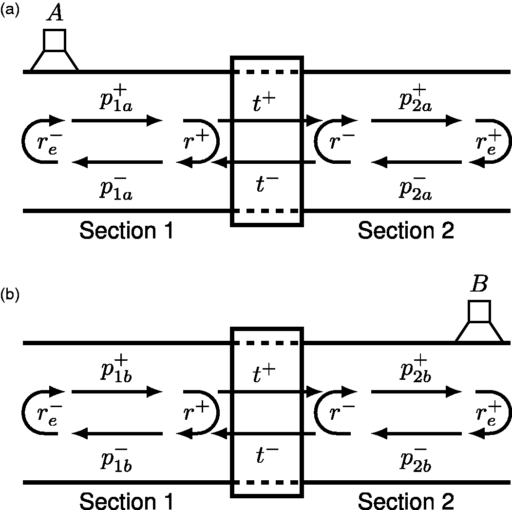
Illustration of the sound field in the duct for measurements A and B by means of the sound pressure amplitudes p, the reflection coefficient r, the transmission coefficient t, and the end reflection re. (a) Measurement A, upstream excitation; (b) measurement B, downstream excitation.
The advantage of combining the two measurements is that the resulting coefficients are independent from the reflection of sound at the duct terminations. These end-reflections are contained in the equations of the sound pressure amplitudes, but do not need to be calculated explicitly. The analysis is applied only in the plane-wave regime (here up to 2100 Hz) i.e., the acoustic pressure is constant across the duct cross-section. The dissipation coefficient of the acoustic energy can be calculated from the reflection and transmission coefficients via an energy balance:

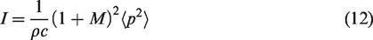
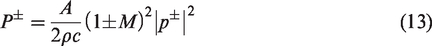
The energy of the incident wave is partly reflected, partly transmitted, and partly absorbed by the damping module. R and T are the power quantities of the reflection and transmission coefficients, while r and t are the corresponding pressure quantities. Blokhintsev
11
defines the acoustic energy flux I in a moving medium (see as well in Morfey
12
)
Applying equation (13) to R and T in equation (11) and then solving for Δ with A1 = A2, ρ1=ρ2, c1 = c2, and
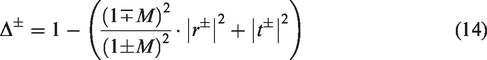
This is an integral value of the acoustic energy that is absorbed while a sound wave is passing the damping module.
Figure 9 presents the dissipation coefficient of the
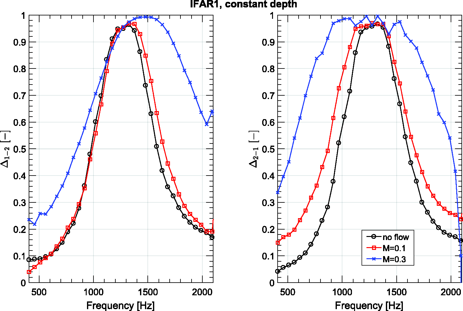
Dissipation coefficient of
no flow
centerline Mach number: 0.1
centerline Mach number: 0.3
The left side of Figure 9 shows the dissipation coefficient in the downstream direction, which is in the no flow case (black line) almost identical to the dissipation values in the upstream direction (right side of Figure 9) since the liner sample is symmetric. It provides a resonator liner typical, distinct dissipation maximum here at around 1300 Hz, which broadens with increased grazing flow Mach number. This frequency is presumably related to a quarter-wavelength (
The dissipation coefficient of the axially segmented
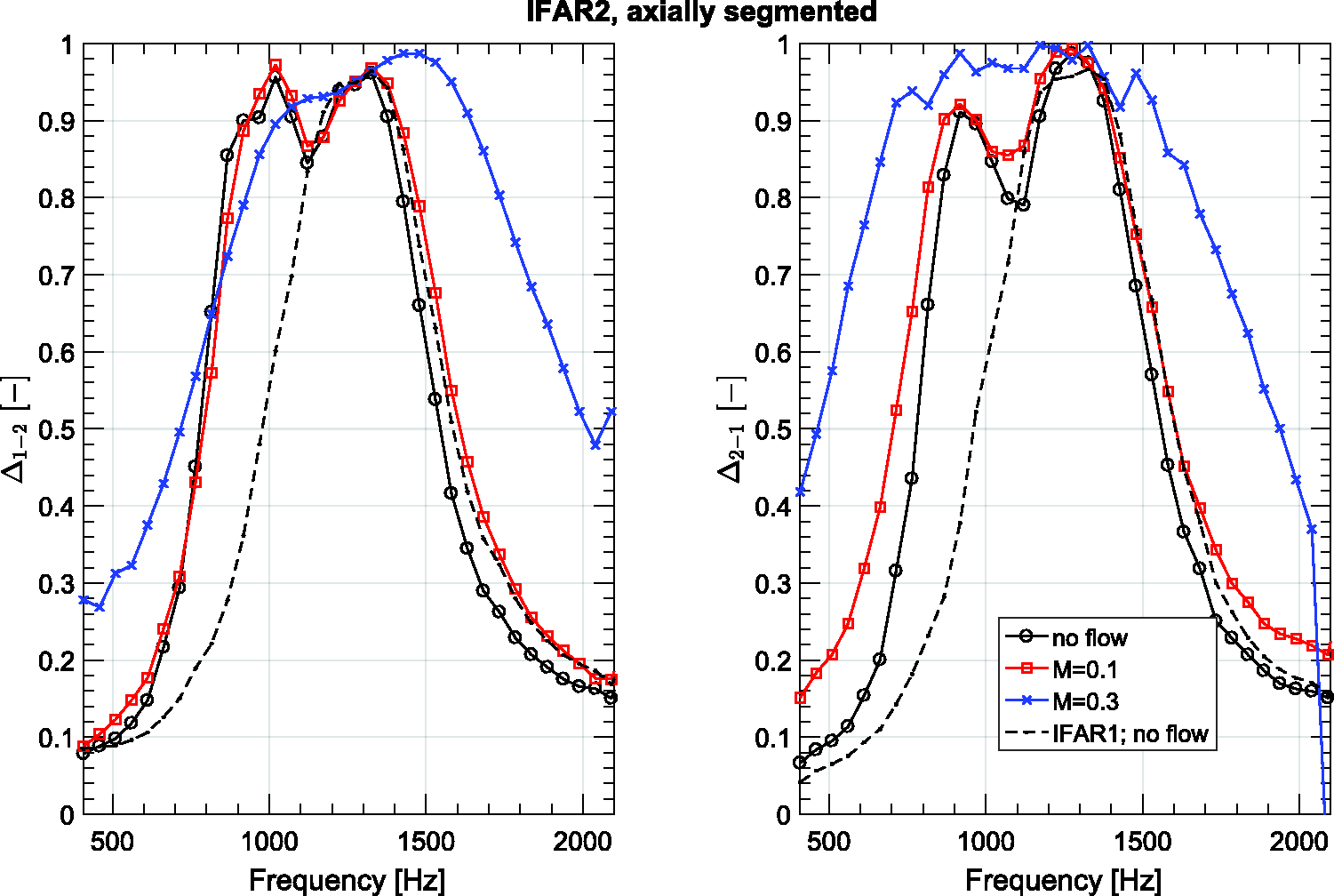
Dissipation coefficient of
Axial pressure profiles
In order to enhance the understanding of the damping characteristics and to prepare the wave number determination in the lined duct sections, Figures 11 (
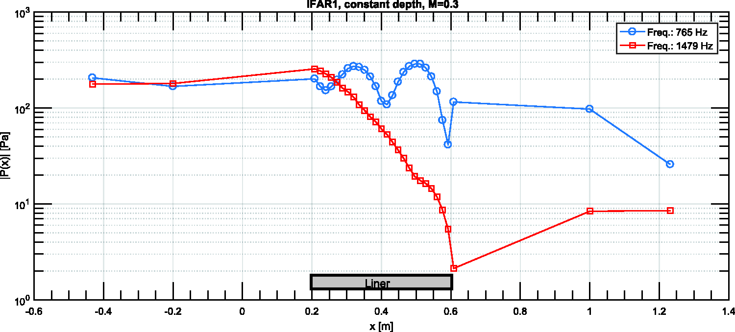
Axial pressure profiles with
The magnitude of the sound pressure for the
The
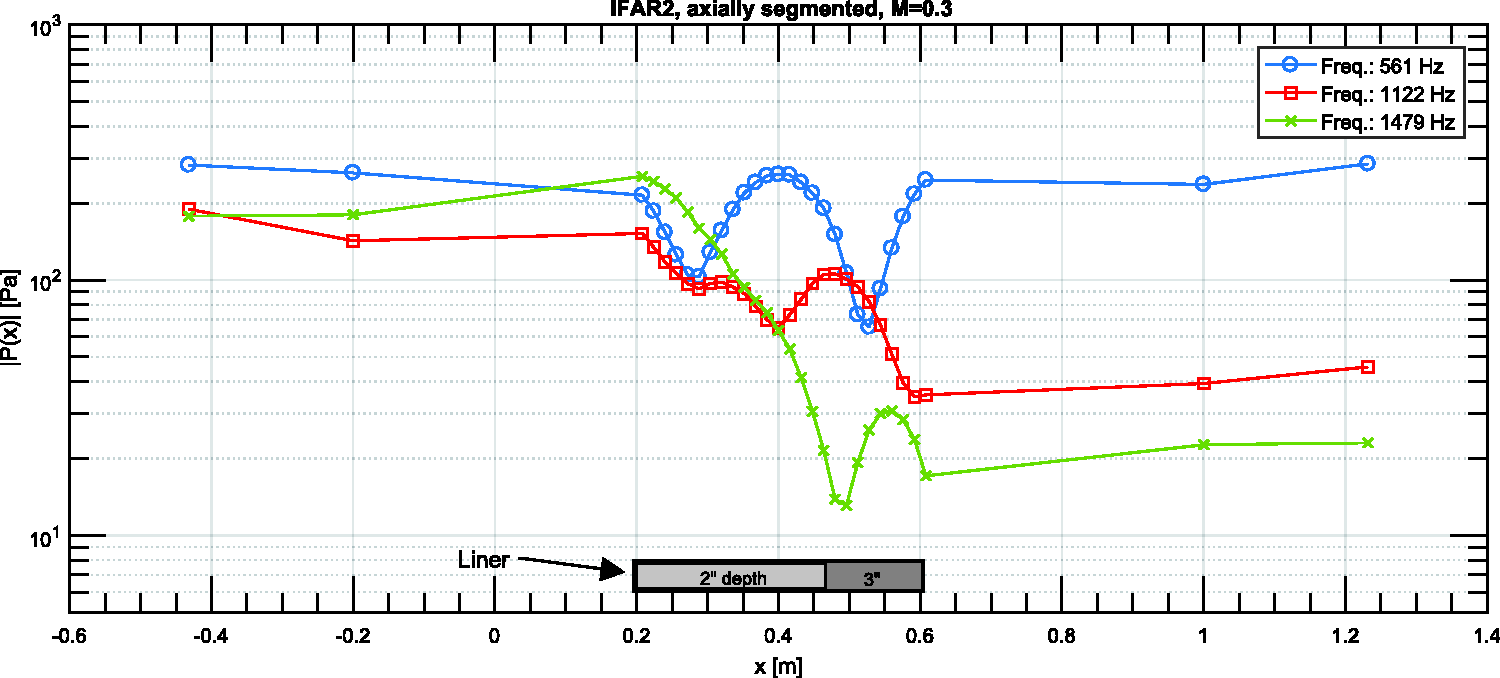
Axial pressure profiles with
Wave number determination
The next step toward the impedance eduction is the determination of the axial wave numbers of all existing modes in the lined section. Here, a combination of two different methods (Kumaresan and Tufts (KT) method and Matrix Pencil (MP) method) combined with a manual sorting procedure was applied. The KT and MP methods are explained in detail in Weng et al.6,13,14 and are only briefly introduced here.
The
While the KT method finds the system poles in two steps (solving the linear system of prediction equations and finding the roots of the prediction polynomial), the
The careful determination of the dominating wave numbers becomes extremely important when a so called “mode crossing” appears in the lined section. “Mode crossing” denotes the change of the least attenuated mode from the fundamental mode (“plane wave”) to a next higher order mode above a certain frequency. This higher order mode is then less damped than the fundamental mode. This effect was observed especially at liner samples with a low resistance value and earlier described for example in detail by Schulz et al. 16
Here, this mode crossing also appears in the no flow and low Mach number flow cases for the
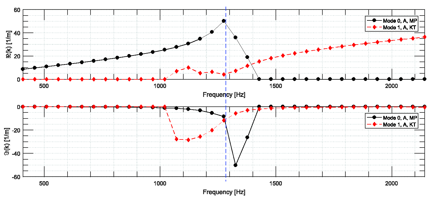
Real part (above) and imaginary part (below) of the determined wave numbers for
Impedance eduction from DLR measurements and comparison to NASA results
In general the test rig setup and the test procedure at the DUCT-R allows different techniques, modal based and nonmodal based, to educe the impedance. A comparative study of these methods was presented in earlier work. 6 In the framework of this IFAR liner benchmark the primary focus was set on the modal based techniques applying the determined wave numbers as described above.
Following the description of the acoustic pressure field for each mode by
Once the wave number
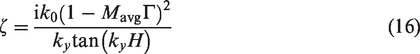
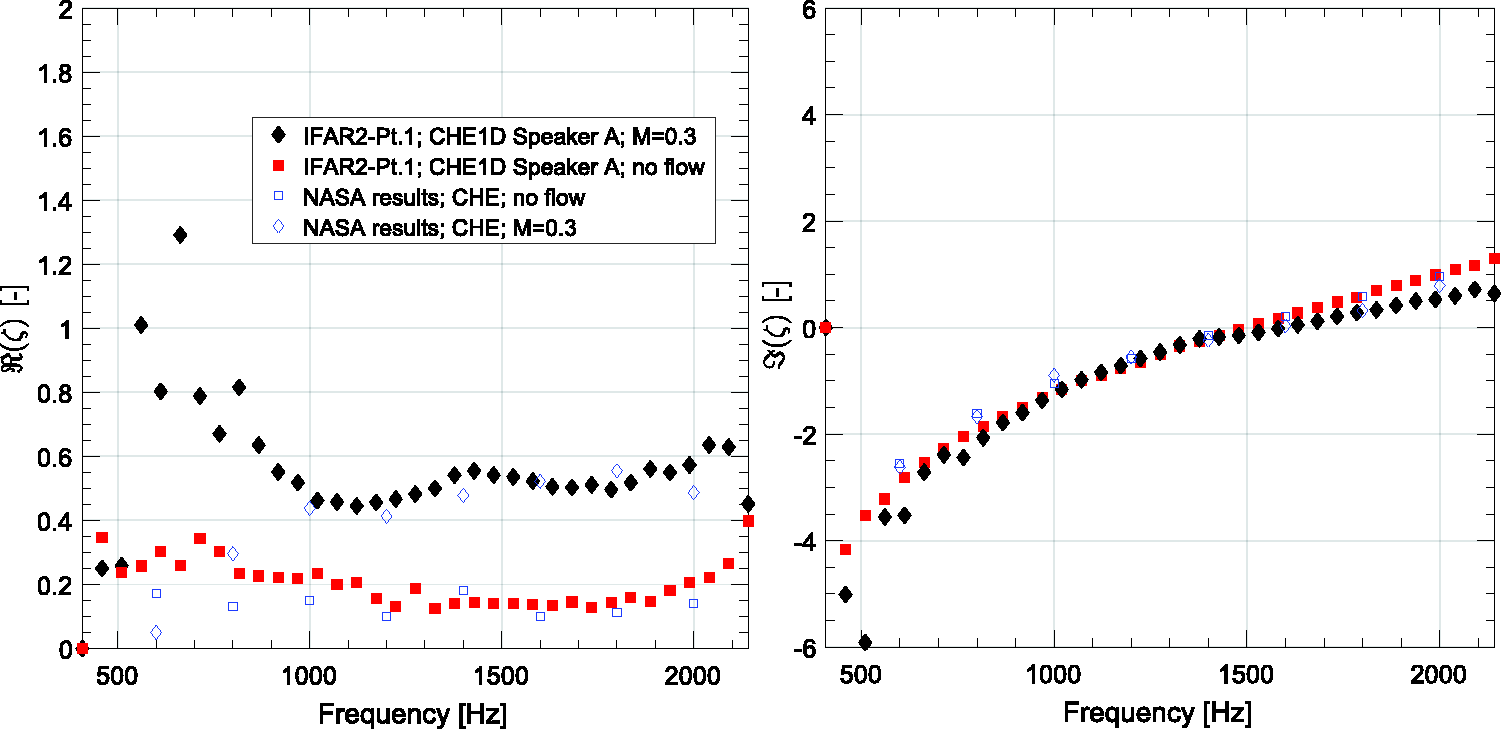
The impedance results obtained by DLR for the
Real part (resistance; left) and imaginary part (reactance; right) of the educed liner impedance from DLR measurements for the
The corresponding values from the NASA GFIT test rig are also plotted in Figure 14 for the no flow case (green triangles) and for the case with a centerline Mach number of M = 0.3 (orange triangles). It should be noted that even with the same measured centerline Mach number the spatial Mach number distribution in the duct cross section is most likely somehow different between the GFIT test rig and the DUCT-R due to the different cross-sectional dimensions and the different axial duct length. However, the comparison of the resistance (Figure 14, left) and reactance (Figure 14, right) data show a very close match between DLR and NASA results. Only for lower frequencies below around 800 Hz some deviations (in the order of 30% for the reactance and the resistance with flow Mach number of 0.3) can be observed.
For the
Figure 15 displays the impedance values for the first liner segment of
Real part (resistance; left) and imaginary part (reactance; right) of the educed liner impedance for the first part of the
The impedance for the second part (
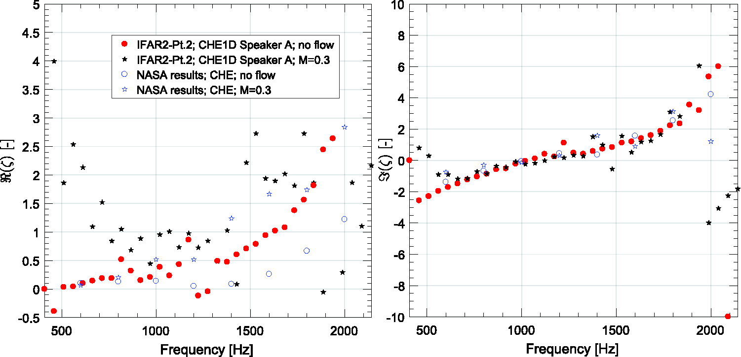
Real part (resistance; left) and imaginary part (reactance; right) of the educed liner impedance for the second part of the
Comparing the results from the constant depth sample
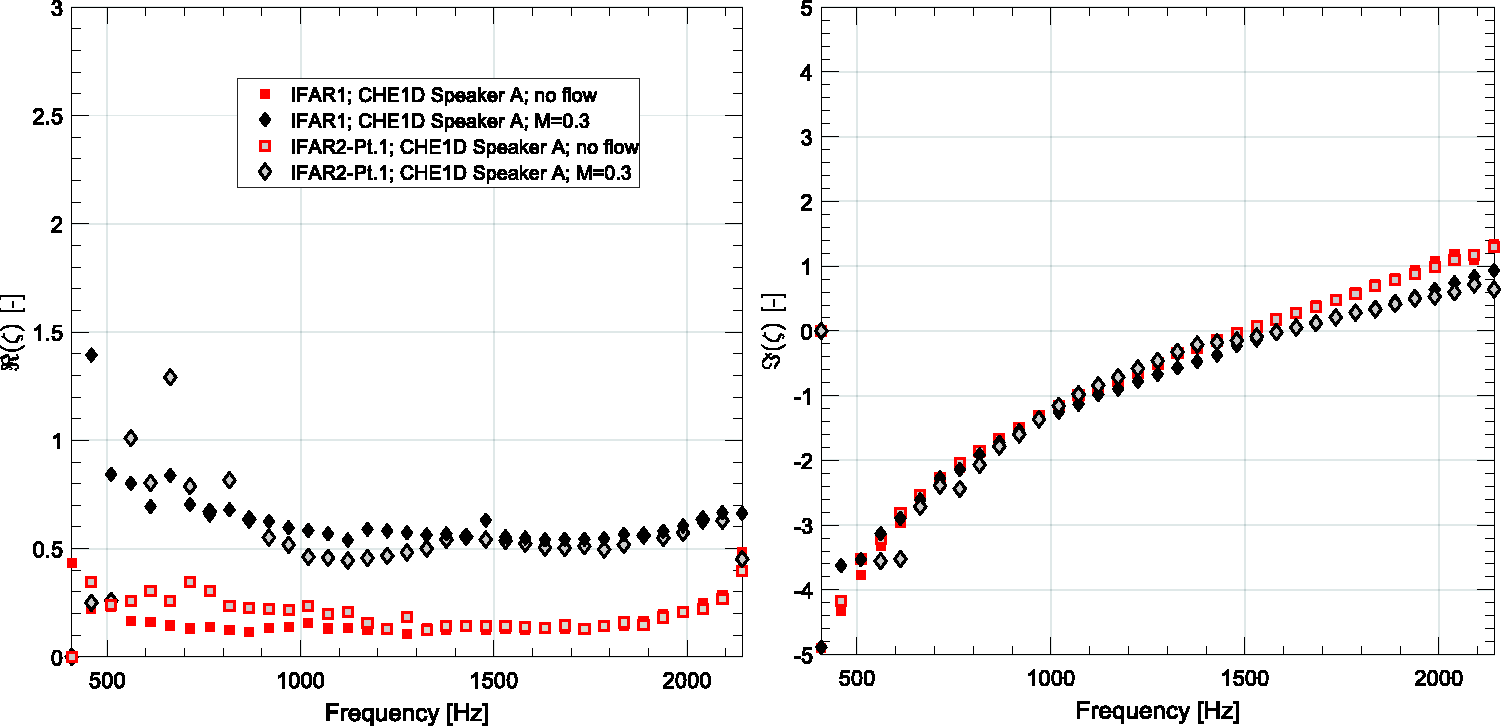
Real part (resistance; left) and imaginary part (reactance; right) of the educed liner impedance for the
Conclusion
In the framework of the IFAR liner benchmark Challenge #1, the comparison of the DLR to the NASA results was presented. Starting with the DLR additive manufacturing and test rig integration of two different liner samples – one with constant cavity depth (
The
The corresponding axial pressure profiles confirm this observation and provide some insight into the total sound pressure level at each microphone position for the different configurations. One key processing step for the impedance eduction is the determination of the axial wave numbers of the dominating modes in the lined sections. Hereby, a combination of two methods (KT/MP) with a specific truncation algorithm (MDL criterion) was applied to the data of the face-to-face microphones above the lined wall. A crucial processing component is here the manual mode selection based on a plausibility assessment.
Different, modal-based and nonmodal-based impedance eduction techniques are available at DLR. For the sake of brevity, only the results of the so-called straightforward method, based on an analytic solution of the one-dimensional Convected Helmholtz Equation (CHE1D), were presented. In this framework, also another modal-based impedance eduction method by solving the Pridmore-Brown equation over the full duct cross-section (PBE-CroSec method) was applied. Although PBE-CroSec takes into account visco-thermal losses as well as shear flow effects, in this case the method yields results fairly similar to the CHE1D.
Impedance eduction for the constant depth liner sample
The comparison to the NASA impedance results shows a very good agreement for both liner samples. The overall evaluation demonstrates the liner impedance eduction capability even for complex nonhomogeneous liner samples.
Footnotes
Acknowledgements
The authors highly appreciate the support of Wolfram Hage and Sebastian Kruck in carefully manufacturing and post processing the liner samples.
Declaration of conflicting interests
The author(s) declared no potential conflicts of interest with respect to the research, authorship, and/or publication of this article.
Funding
The author(s) received no financial support for the research, authorship, and/or publication of this article.