Sage Journals: Discover world-class research

Abstract

Several techniques are available to characterize acoustic liners when subject to grazing flow and high sound pressure level (SPL). Although the in situ technique started as the primary experimental procedure, impedance eduction techniques have gained popularity over the past years. However, there is a lack of comparison between these group of methods, especially at conditions typically found in turbofan engines. In this work, in situ and impedance eduction techniques are compared at high flow velocities and SPL using typical acoustic liner test samples and considering uniform flow. Both upstream and downstream acoustic wave propagation will also be considered in view of the discrepancies recently observed by eduction methods. A new method to compensate the instrumentation effect in the in situ technique is proposed and validated. Results are obtained for bulk Mach numbers up to 0.5 and SPLs up to 145 dB for both in situ and two eduction techniques. The three methods presents good agreement in the absence of flow. Unexpected results are observed with higher flow Mach numbers using the eduction technique.

Keywords

Acoustic liners acoustic impedance measurement impedance eduction in situ impedance experimental duct acoustics

Introduction

Acoustic liners are commonly used to suppress tonal and broadband noise components in turbofan aeroengine applications. Typical liner geometry consists of a honeycomb structure between a hard backplate and a perforated facesheet. These are typically represented by its acoustic impedance, and therefore accurate estimates of this parameter are required. The acoustic impedance of liners is known to depend on its geometry (e.g. core width, percentage of open-area and hole diameters) and operational conditions (e.g. sound pressure level (SPL) and grazing flow Mach number).¹

Although the acoustic impedance is simply defined by the ratio of the complex acoustic pressure and the complex normal acoustic particle velocity, both on the lined surface, measuring these quantities is not a trivial task. Dean² first proposed an installation of a pair of microphones at the facesheet and backplate of the same honeycomb cell, as schematically shown in Figure 1 (see the detail). A simple relation can be derived for the acoustic field inside the cell, such that the liner impedance can be inferred from the complex acoustic pressures at the facesheet and backplate. In general, the perforate facesheet is not always perfectly aligned with the honeycomb walls such that each cell may have slightly different percentage of open area, and consequently a different acoustic impedance. Hence, a group of experimental indirect methods has been developed over the past decades (e.g.^3–6). The so-called impedance eduction techniques rely on measurements of the acoustic field inside the duct and the consideration of suitable governing equations and boundary conditions. These methods can be divided in two subgroups. Inverse eduction methods are based on the minimization of the difference between the measured acoustic field to the numerically calculated acoustic field with an impedance estimation.³ The direct eduction methods allows the impedance evaluation by means of the wavenumber of the lined section extracted using Prony-like algorithms.⁷

Figure 1.

Schematic view of the measurement apparatus for liner impedance with grazing flow (both in situ and eduction techniques).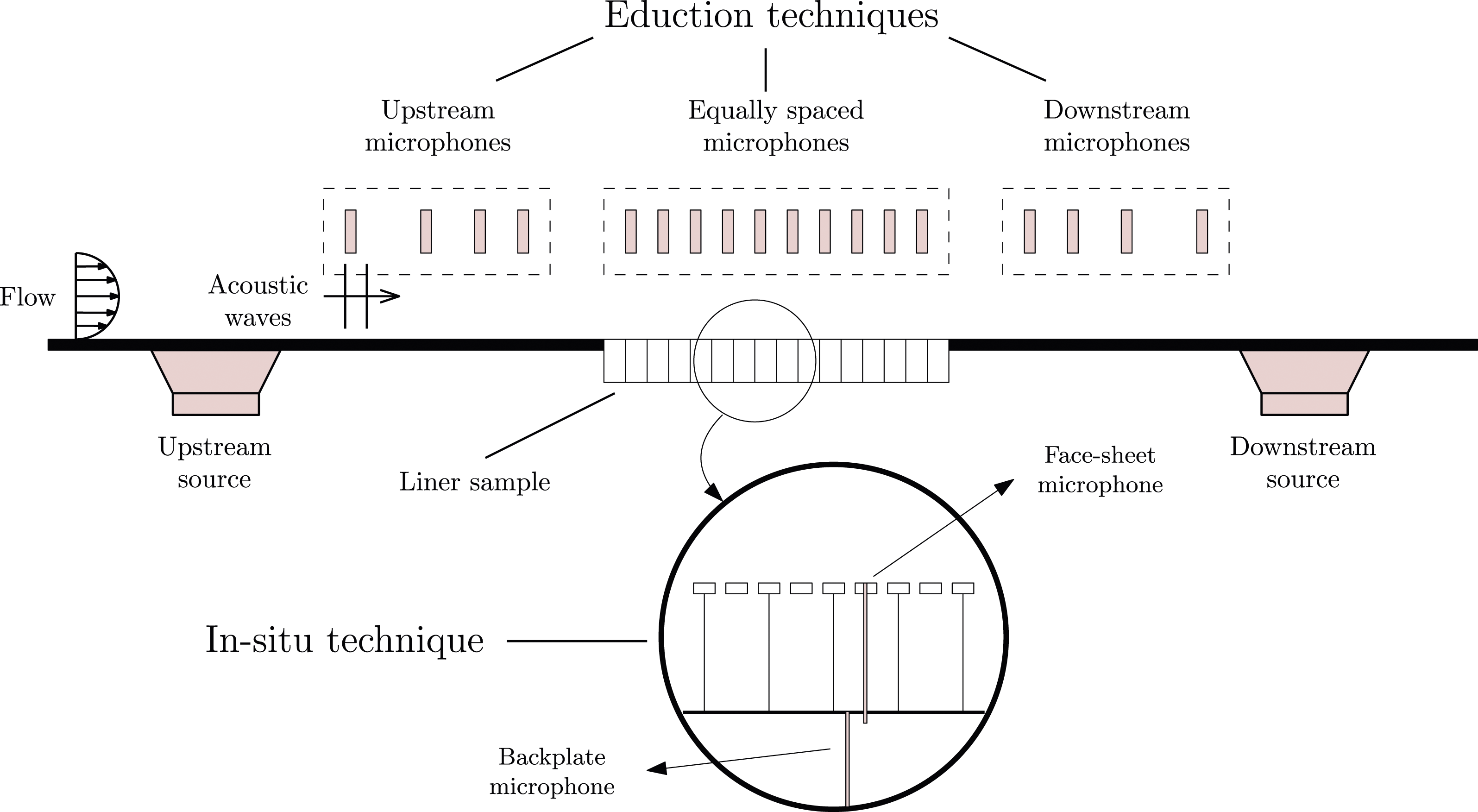

Ferrante et al.⁸ compared the in situ with an impedance eduction technique based on the two-port matrix (for both no-flow and grazing flow conditions) and with a normal incidence impedance tube (only no-flow). The results suggested good agreement between the in situ technique with both reference methods, although some discrepancies were observed, especially with grazing flow. Bodén et al.⁴ used both in situ and impedance eduction techniques to compare results obtained with upstream and downstream propagation. Results have shown that the unexpected difference in the measured impedance with different source locations is observed with both methods. However, the results obtained with the in situ technique do not follow the same pattern in comparison to those obtained via impedance eduction, that is the in situ resistance is nearly constant with frequency, whereas the educed resistance shows a strong frequency-dependence. Serrano et al.⁹ also compared the in situ technique with three impedance eduction methods. Good agreement was also observed for the results obtained with the different eduction methods, but it is less evident for the in situ results. The results obtained with the in situ technique again showed different trends in comparison to the educed ones.

In this work, we compare in situ and impedance eduction techniques at high grazing flow and SPL, for average grazing flow Mach numbers up to 0.5 and SPL at the liner facesheet up to 145 dB and for both upstream and downstream conditions. For the in situ technique, we revisited typical instrumentation methods and compare miniature microphones with capillary-probes. Also, we investigate a correction available in the literature, proposing a new methodology to compensate for the instrumentation effect. For an inverse eduction technique, a numerical model of the acoustic field is computed using the mode-matching method. Also, a direct impedance eduction technique based on the Kumaresan and Tufts (KT) algorithm¹⁰ is used.

This document is organized as follows. First, we describe in detail the experimental techniques. In what follows, we present the experimental setup at the Federal University of Santa Catarina (UFSC). Next, the preparation for in situ measurements and a discussion regarding instrumentation and the necessary correction are presented. In section Results and Discussion, the primary results are shown and the difference observed between the methods is discussed. Finally, the conclusions are outlined in the final section.

Experimental techniques

In situ technique

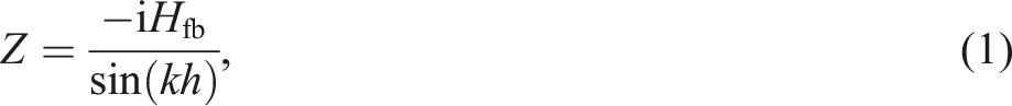
The in situ measurement technique estimates the acoustic particle velocity at the facing sheet and the cell impedance using the measurements of the acoustic pressure at the facing sheet and backing sheet. The main assumptions of the technique are that: (i) the backplate is totally reflective, and (ii) only standing plane waves exist in the honeycomb cell. With these conditions, it can be shown that the in situ impedance is given by²

Z = \frac{- i H_{fb}}{\sin (k h)},

(1)

where Z is the specific acoustic impedance normalized by ρ₀c₀,

i = \sqrt{- 1}

is the imaginary unit, H_fb is the ratio between complex acoustic pressures at the facesheet and backplate, k = ω/c₀ is the free-field wavenumber and h is the cavity height.

The in situ technique implicitly assumes that the liner is locally reactive, and no assumptions regarding the flow outside the liner are made. Therefore, it does not rely on the definition of a boundary condition such as Ingard–Myers boundary condition^11,12 since it does not attempt to model the acoustic field as performed in the impedance eduction techniques.

Impedance eduction

For inverse impedance eduction techniques, a numerical model of the acoustic field inside the duct is necessary. Finite-Element and Discontinuous Galerkin methods are often employed to simulate the entire domain (e.g. Watson and Jones³ and Roncen et al.⁶). However, we can take advantage of the modal structure of the acoustic field to compute much faster solutions, which are particularly important for the application of iterative routines used to educe the liner impedance. In this context, the mode-matching method can reproduce solutions obtained with the Finite-Element Method.¹³ In the present work, a mode matching technique will be used to match the solutions of the 2D-convected Helmholtz equation on the hard/lined duct interfaces.

Governing equations

The considered coordinates system and relevant duct parameters are presented in Figure 2. We assume a uniform parallel flow in the positive z direction such that the acoustic pressure perturbation $p \propto \hat{p} \exp (i ω t - i k_{z} z)$ is governed by the Convected Helmholtz Equation,

(\nabla_{⊥}^{2} + {(k - M k_{z})}^{2} - k_{z}^{2}) \hat{p} = 0,

(2)

where M ≡ U/c₀ is the flow bulk Mach number, and k_z is the axial wavenumber. In this work, we can neglect wave propagation in the y direction in the frequency range of interest,¹³ so that

\nabla_{⊥}^{2} \equiv \frac{d^{2}}{d x^{2}}

Figure 2.

Coordinate system and duct geometry for the impedance eduction technique.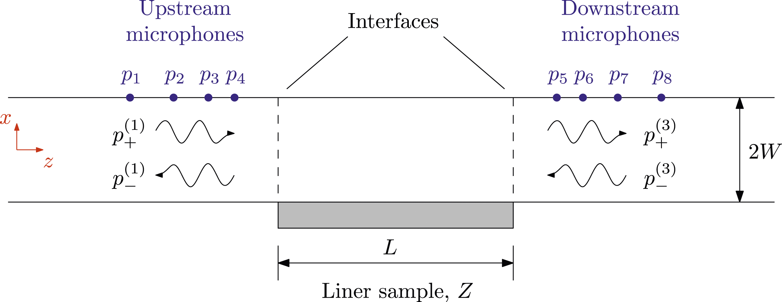

At x = W, the rigid wall boundary condition implies $\frac{d \hat{p}}{d x} = 0$ . At x = −W, the Ingard–Myers boundary condition^11,12 is assumed,

\frac{d \hat{p}}{d x} = \frac{i}{k Z} {(k - M k_{z})}^{2} \hat{p} .

(3)

Mode-matching method

At each section j, the acoustic field p (x, z) can be approximated by a sum of $N$ acoustic modes,

p^{(j)} (x, z) = \sum_{n = 1}^{N} (A_{n}^{(j) +} ψ_{n}^{(j) +} (x) \exp (- i k_{z, n}^{(j) +} z) + A_{n}^{(j) -} ψ_{n}^{(j) -} (x) \exp (- i k_{z, n}^{(j) -} z)),

(4)

where A_n are the modal amplitudes, ψ(x) are the mode shapes, and + and − denote downstream and upstream propagating modes, respectively. In order to determine the axial wavenumbers and mode shapes supported at each section, we rewrite the Convected Helmholtz equation as

(\frac{d^{2}}{d x^{2}} + k^{2}) \hat{p} = k_{z} (2 k M + (1 - M^{2}) k_{z}) \hat{p},

(5)

which is a suitable form to solve as a generalized eigenvalue problem,

A x = k_{z} B x

(6)

where

x \equiv {[{\hat{p}}_{i}, {\hat{q}}_{i}]}^{T}, i = 0, \dots, N

contains the discrete set of pressure points in the transverse direction and the auxiliary variable

\hat{q} = k_{z} \hat{p}

. This problem is solved using the pseudospectral method, which can be interpreted as a N-th order finite difference method¹⁴ p. 98. The collocation points follow a Gauss-Lobatto grid distribution¹⁴ p. 570, and boundary conditions are applied at rows corresponding to i = 0 and i = N. More details about the matrices A and B can be found in Spillere et al.¹³ In general, N = 100 provides excellent accuracy for the purposes of this work.

Once the eigenvalues and eigenvectors are known, the modal amplitudes at each section can be determined by matching mass and momentum at each interface,¹⁵

(1 - M^{2}) \int_{S} \bar{f} (p^{(s + 1)} - p^{(s)}) d S - \frac{M^{2}}{i k} \oint_{Γ} \bar{f} (\frac{p^{(s + 1)}}{Z^{(s + 1)}} - \frac{p^{(s)}}{Z^{(s)}}) d Γ = 0,

(7a)

(1 - M^{2}) \int_{S} \bar{f} (u^{(s + 1)} - u^{(s)}) d S + \frac{M}{i ρ_{0} c_{0} k} \oint_{Γ} \bar{f} (\frac{p^{(s + 1)}}{Z^{(s + 1)}} - \frac{p^{(s)}}{Z^{(s)}}) d Γ = 0,

(7b)

where s = 1, 2 are the rigid/lined and lined/rigid interfaces, S is the duct cross-section, Γ is the interface contour and

\bar{f}

is the complex conjugated test function. In practice, closed-form solutions are known for the integrals in equations (7a) and (7b) which improves accuracy and reduces computational cost (see Spillere et al.¹³ for details). Substituting equation (4) into equations (7a) and (7b) leads to a system of equations that can be solved for the modal amplitudes.

Inverse eduction procedure

The impedance eduction procedure described in this work is iterative: an impedance guess is necessary to compute the numerical acoustic field $p_{q}^{num}$ at each microphone location z_q, which is compared to the measured acoustic field $p_{q}^{\exp}$ by means of the following cost function

F (Z) = \sum_{q = 1}^{8} | \frac{p_{q}^{\exp} - p_{q}^{num} (Z)}{p_{q}^{\exp}} | .

(8)

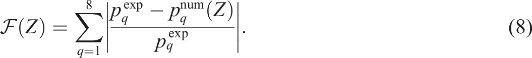
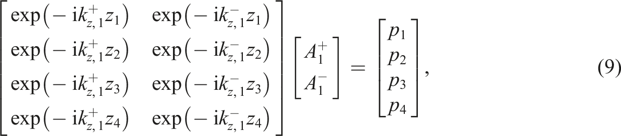
The Levenberg–Marquadt algorithm^16,17 is used to minimize this cost function, which leads to the liner impedance. In order to improve convergence, semi-empirical impedance models (e.g. Murray and Astley¹) are commonly employed as an initial guess for the liner impedance. The inputs to this procedure are the plane-wave amplitudes propagating towards the lined section. These can be found by means of an over-determined plane wave decomposition procedure, for example in the upstream section

[\begin{array}{l} \exp (- i k_{z, 1}^{+} z_{1}) & \exp (- i k_{z, 1}^{-} z_{1}) \\ \exp (- i k_{z, 1}^{+} z_{2}) & \exp (- i k_{z, 1}^{-} z_{2}) \\ \exp (- i k_{z, 1}^{+} z_{3}) & \exp (- i k_{z, 1}^{-} z_{3}) \\ \exp (- i k_{z, 1}^{+} z_{4}) & \exp (- i k_{z, 1}^{-} z_{4}) \end{array}] [\begin{array}{l} A_{1}^{+} \\ A_{1}^{-} \end{array}] = [\begin{array}{l} p_{1} \\ p_{2} \\ p_{3} \\ p_{4} \end{array}],

(9)

and similarly for the downstream section. The plane wave axial wavenumber

k_{z, 1}^{\pm} = \pm k K_{0} / (1 \pm K_{0} M)

also accounts for viscothermal losses at the duct walls given by the first order Kirchhoff solution K₀.¹⁸

Direct eduction procedure - KT algorithm

In this work, the KT algorithm is used to extract the axial wavenumber from microphone measurements. The algorithm consists in fitting a linear combination of damped complex exponentials to the recorded pressure at uniformly spaced locations. For flush-mounted microphones opposite to the liner sample (test section j = 2), one can write the acoustic pressure simply as

p_{m}^{(2)} (z) = \sum_{n = 1}^{N} (A_{n}^{(2) \pm} \exp (- i k_{z, n}^{(2) \pm} m Δ z)), for m = 0,1, \dots, M - 1,

(10)

where

p_{m}^{(2)}

is the pressure at the m − th microphone, Δz is the distance between two consecutive microphones and

M

is the number of microphones at the lined section. Assuming that the acoustic field in the lined section is dominated by

N

modes and choosing a convenient model order

L

which satisfies

N \leq L \leq M - N

, the equation (10) becomes

p_{m + r}^{(2)} (z) = \sum_{n = 1}^{L} (A_{n}^{(2) \pm} \exp (- i k_{z, n}^{(2) \pm} (m + r) Δ z)), for r = 0, \dots, M - L - 1 .

(11)

In this work, we consider a model order of $L = 3 M / 8$ , as proposed by Renou and Aurégan.¹⁹

If a_i are the coefficients of the characteristic polynomial,

\sum_{m = 0}^{L} a_{i} \exp (- i k_{z, n}^{(2) \pm} m Δ z) = 0,

(12)

then it is possible to show that

\sum_{m = 0}^{L} a_{i} \exp (- i k_{z, n}^{(2) \pm} (m + r) Δ z) = 0,

(13)

or, in the matrix form

H a = - b,

(14)

where

H = [\begin{array}{l} p_{1} & p_{2} & \dots & p_{L} \\ p_{2} & p_{3} & \dots & p_{L + 1} \\ ⋮ & ⋮ & ⋱ & ⋮ \\ p_{M - L} & p_{M - L + 1} & \dots & p_{M - 1} \end{array}], a = [\begin{array}{l} a_{1} \\ a_{2} \\ ⋮ \\ a_{L} \end{array}], b = [\begin{array}{l} p_{0} \\ p_{1} \\ ⋮ \\ p_{M - L - 1} \end{array}],

(15)

which is solved for the polynomial coefficients a in a least square sense. Applying the KT algorithm, spurious poles are removed by performing a SVD on matrix H,

H = U S V^{H},

(16)

where U and V are unitary matrices, S contains the σ_i singular values of H on the main diagonal, and V^H denotes the conjugate transpose of V. The reduced rank approximation of H is then given by

H_{Q} = U S_{Q} V^{H},

(17)

where only the first Q singular values are considered, such that σ_i = 0 for i > Q. Therefore, the coefficients of the polynomial can be found by

H_{Q} a = - b .

(18)

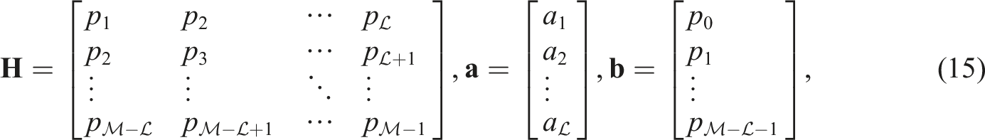
The choice of Q is not trivial since this parameter may depend on frequency, test sample and flow velocity. In this work, we followed the minimum description length (MDL) criterion as presented in Weng et al.²⁰

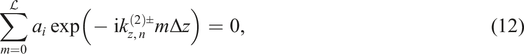
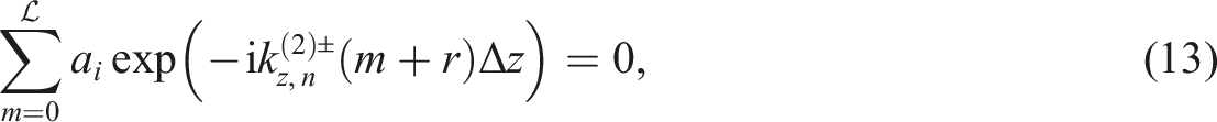
From equation (18) solution, the system zeros V_n are given by the roots of equation (12), with a₀ = 1. Finally, the axial wavenumbers are computed from

k_{z, n} = \frac{\ln (V_{n})}{- i Δ z} .

(19)

Since $L$ roots are found, the most accurate physical wavenumber must be selected to compute the liner impedance. In this work, we selected the least attenuated mode, following Watson et al.⁷

Experimental setup

UFSC liner test rig

The UFSC Liner Test Rig is composed of five modular sections containing compression drivers, microphones and a sample holder, as can be seen in Figure 3. A compressed air system supplies grazing flow with average Mach number up to 0.6. Acoustic sources are found on both upstream and downstream sides of the sample holder, allowing acoustic propagation in the same direction and against flow. The test section has a rectangular cross-sectional area of 40 mm height by 100 mm width, and anechoic terminations are located upstream and downstream of the test section, with a reflection coefficient below 0.2 in the frequency range of interest and absence of flow.

Figure 3.

Representation of UFSC liner test rig.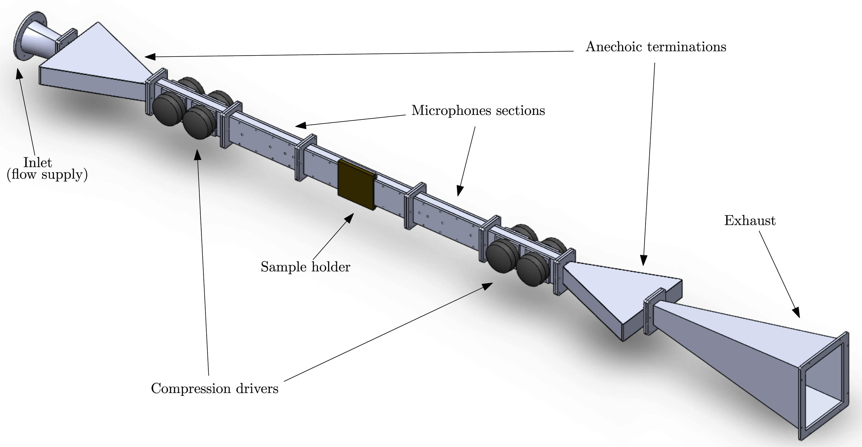

Two arrays of four flush mounted B&K 4944-A 1/4” microphones in the lower hard walled upstream and downstream the sample holder section allows acoustic field measurement for the iterative eduction procedure. Another array of eight flush mounted microphones is located at the hard wall opposite to the liner sample, for the KT-algorithm based eduction method. The microphone membranes are on the hard wall plane, therefore no correction is required for this type of installation. The microphones are placed centered in the duct width, which allows only plane measurement bellow the second order mode cut-on frequency along the width of the duct. For the in situ measurement, a pair of Kulite MIC-062 high intensity microphones is used, as shown in Figure 4(a). Four beyma CP-855Nd compression drivers are placed on both sides of the test section. Excitation signals are amplified by B&K 2716-C power amplifiers.

Figure 4.

Pictures of the different instrumentation used for in situ technique. (a) Kulite holder for the in situ technique. (b) Capillary-tube probe that will be used as alternative to Kulite microphones for the in situ technique.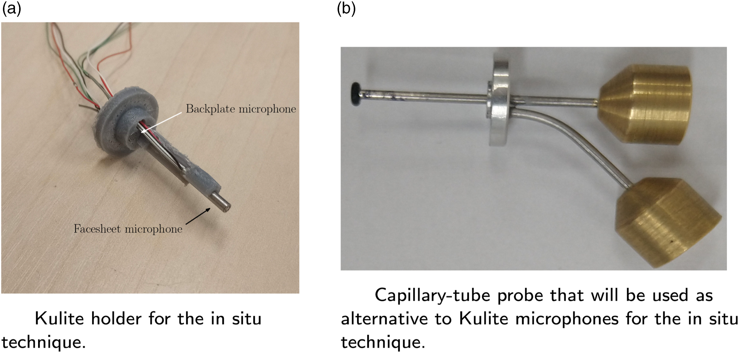

Microphone signals are acquired with sampling rate of 25.6 kHz, simultaneously with acoustic excitation generation on a National Instruments PXI system, controlled by an in-house developed Python3 code. Data is processed with Welch’s method, 30 averages of 25 600 samples with 75% of overlapping. A flat-top window is used, to guarantee tone amplitude accuracy. A loudspeaker excitation signal return is used as noiseless reference for cross-spectrum estimation free from extraneous noise components.

In spite of the practicality of directly measuring the local acoustic field, the use of small-scale microphones is quite a tricky task. The test sample preparation requires a lot of attention and any small deviation is a source of large errors, specially regarding the instrumented cell sealing. In this work, the measurements with small-scale microphones will be compared to capillary-tube probes, instrumented with B&K 4944-A 1/4” microphones as alternative to the traditional Kulite instrumentation. Figure 4(b) shows a pair of probes that will be used in future measurements. The probes were fabricated with 1.6 mm stainless steel capillary, coupled to a brass adapter to positioning the 1/4” microphone.

Both eduction microphones and in situ instrumentation (Kulite microphone pair or capillary-tube probes) amplitude and phase were cross-calibrated with respect to a reference microphone by exposing them to the same acoustic field.²¹ This procedure is important specially to the in situ technique, due to its high sensitivity to possible microphones (or probes) phase shift⁸ and it is going to be described with more detail in Section Calibration procedure and sample preparation.

The temperature inside the test section is measured with a KIMO TM-110 temperature transmitter. Flow speed in the test section inlet is measured by means of a 2 mm diameter Pitot tube, coupled to a KIMO CP-115 differential pressure transmitter. The average Mach number in the test section is known by a pre-calibrated factor, determined by a quadrature averaging method.²²

Test samples

In this study, two typical single degree of freedom liner sample will be used for the experiments, that will be referred as Sample A and Sample B. Sample A has a facesheet thickness of 1 mm, the percentage of open area is 12%, with holes of diameter 1 mm and a honeycomb core height of 25.4 mm. Sample B has a facesheet thickness of 1 mm, the percentage of open area is 7.4%, with holes of diameter 1 mm and a honeycomb core height of 48.6 mm. Both liner samples have a nominal length of 210 mm.

Test conditions

In this work, the following test conditions will be considered. The acoustic sources will be adjusted to reach 130 dB and 145 dB of SPL at the facesheet of the instrumented cell for in situ measurement of the liner sample. The choice for these SPL’s matches the facilities capability, while allowing the evaluation of the linear behaviour of the liner and the non-linear effect due to high SPL. To guarantee maximum SPL at the facesheet probe, the samples are rotated so the instrumented cell is always as close as possible to the acoustic source. The tests will be carried with a no flow condition and with grazing flow with an average Mach number of 0.3 and 0.5, at liner sample section. A stepped pure tone sine over a frequency range from 0.5 kHz to 3.0 kHz is used with a 0.125 kHz frequency step.

In situ instrumentation analysis

In this section, the calibration procedure and sample instrumentation is described. After that, the two instrumentation approaches used for in situ impedance measurement are compared. Also, a discussion is made regarding the correction used to compensate for the volume blockage at the measured liner cavity due to instrumentation and a modification is proposed. For the sake of brevity, in this analysis, only sample B is considered.

Calibration procedure and sample preparation

Due to the high sensitivity of the in situ methodology, a systematic procedure to compensate any amplitude and phase shift between the microphone (or probe) pair is important. This is especially necessary for the case of the probes, since the capillary tubes have their own frequency response function. In this work, we followed the approach of Krishnappa,²¹ which is based on exposing the microphone pair to the same acoustic field and then using the frequency response function between the two acquired signals as a correction for the measured H_fb. This was achieved by positioning the microphones at a rigid end of an acoustic tube, as pictured in Figure 5. A reference microphone is also positioned at the duct end so the facesheet microphone (or probe) can be calibrated with respect to the absolute amplitude, which allows evaluation of the SPL at the measuring position. The duct has a diameter of 25.4 mm and is 1 m long, which guarantees that only plane waves are propagating towards the microphones. The frequency response functions were obtained by means of the H₁ estimator²³ using pure tones as in the measurements, but with 300 averages of 25 600 samples with 75% of overlapping.

Figure 5.

Probe pair calibration.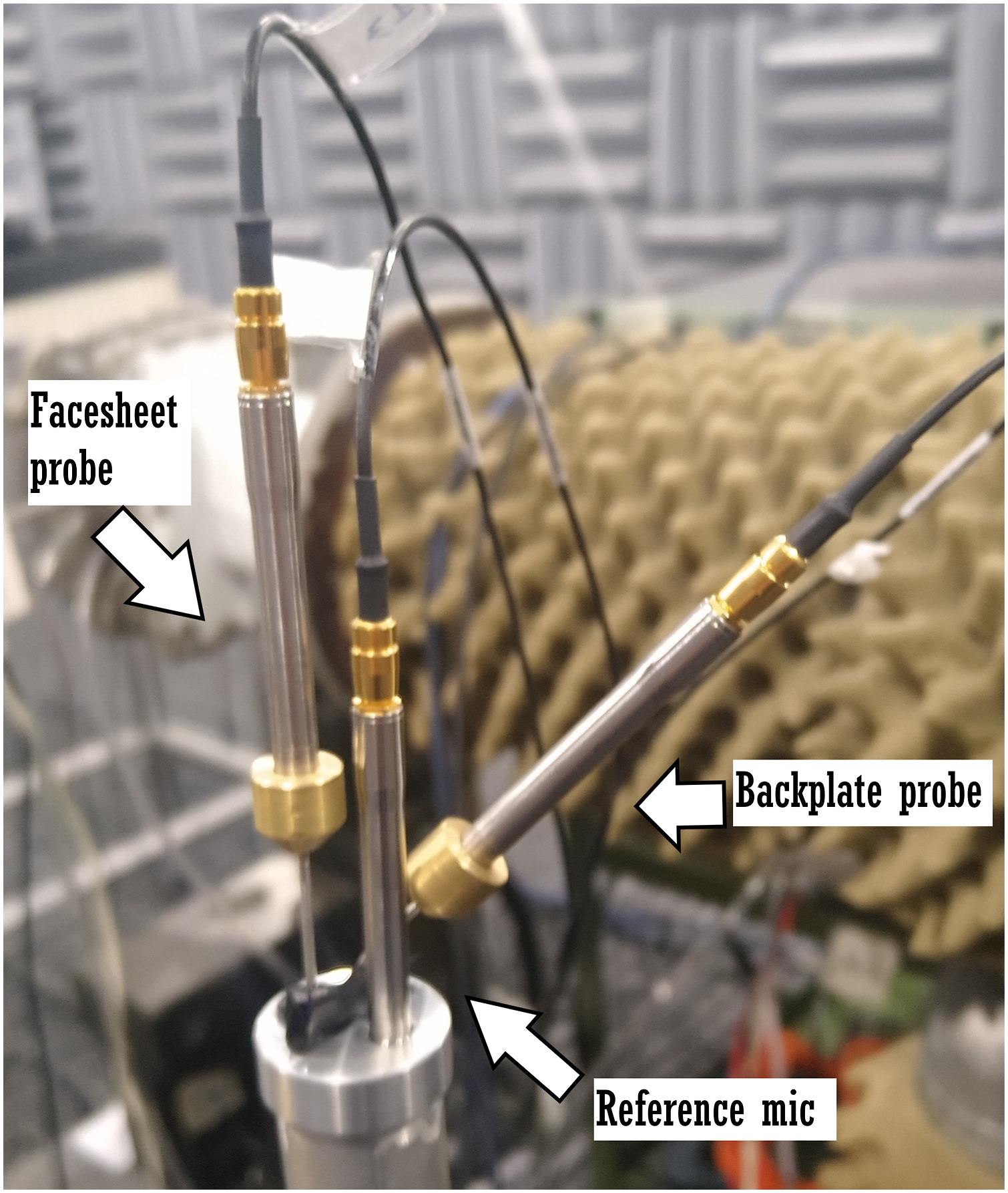

The capillary-tube probes are similar to a closed-open tube. Therefore, resonances are expected at frequencies close of odd multiples of one quarter of wavelength. In this scenario, precisely evaluating the frequency response function became difficult. An alternative procedure is to place an absorbent material inside the tube. In this work, we placed acoustic foam in the final quarter of end of the tube closest to the microphone, where the acoustic pressure is expected to be highest at the resonance. The frequency response functions with the reference microphone as the reference for the H₁ estimator for a pair of probes with and without foam seen in Figure 6. The foam was inserted for all of the subsequent impedance measurements.

Figure 6.

Probe pair frequency response function with and without foam. The facesheet (FS) probe is straight and its capillary tube is 70 mm long. The backplate (BP) probe is curved and its straightened length is approximately 30 mm.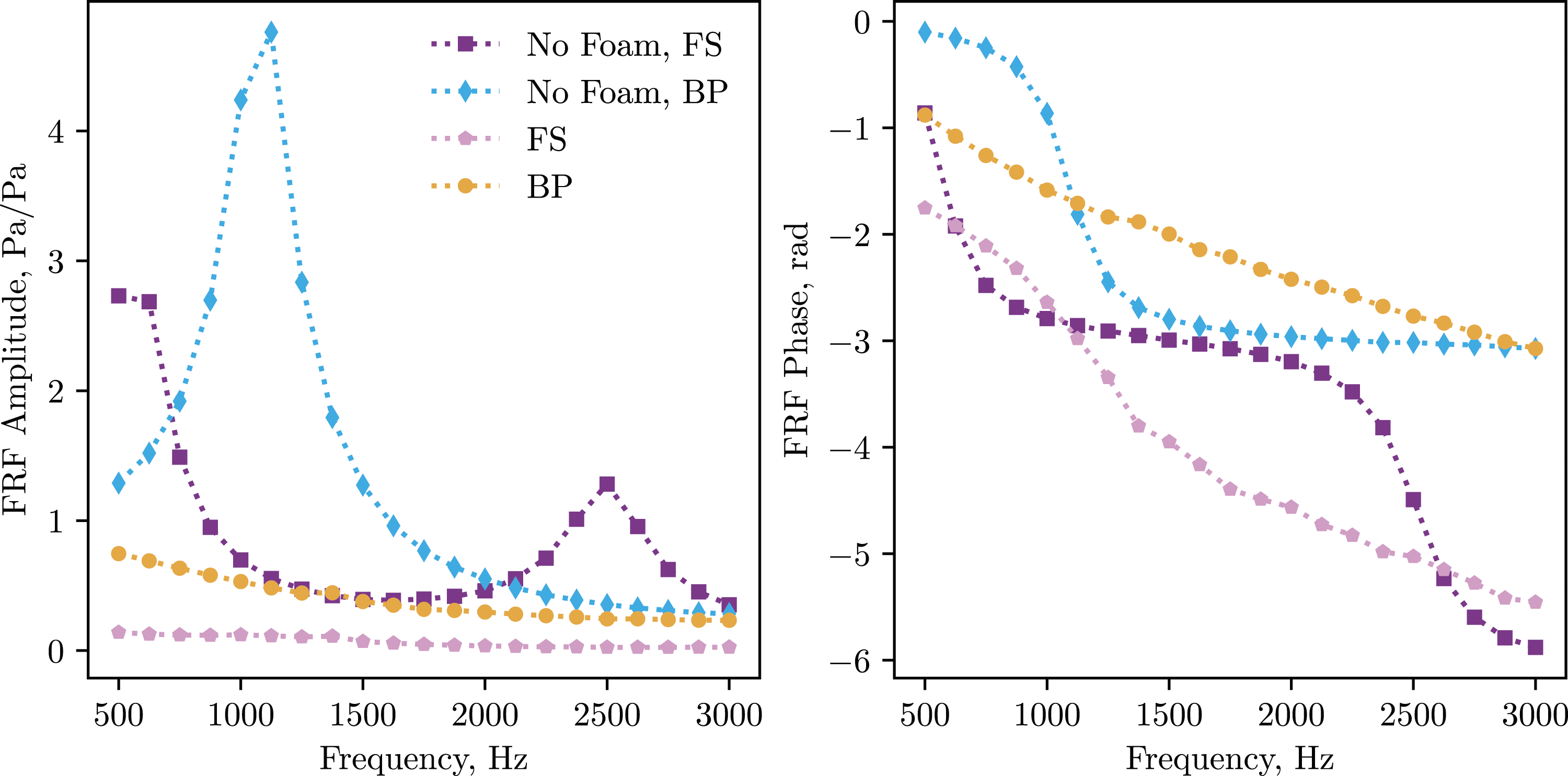

The liner cell is expected to behave as a rigid cavity. Therefore, it is necessary to guarantee that the instrumented cell is sealed, otherwise pressure leakage may lead to unexpected results, especially at lower frequencies, since the cavity impedance is expected to be the dominant component.²⁴ Hence, the holders that we used for both the Kulites or the probes, was bonded to the sample backplate with epoxy. The Kulite holder has an extra challenge, since there is a hole to pass the cables of the facesheet microphone. This hole was sealed using bee-wax, and its efficiency was verified by comparing the results with a predictive model, as will be discussed in the following section.

No-flow results

Figure 7 shows the results obtained with both instrumentations for the in situ technique, not applying any correction to the measured impedance. The experimental results are compared to the predicted impedance obtained by means of the semi-empirical model from Yu et al.²⁵ ¹ Since this model was tuned with in situ measurements, good agreement is expected.

Figure 7.

Comparison of measured impedance using the in situ technique and differing instrumentation. No correction applied to data. “UTAS Model” refers to semi-empirical model from Ref.²⁵ Results for sample B for facesheet SPL of 130 dB, abscence of flow and upstream acoustic source.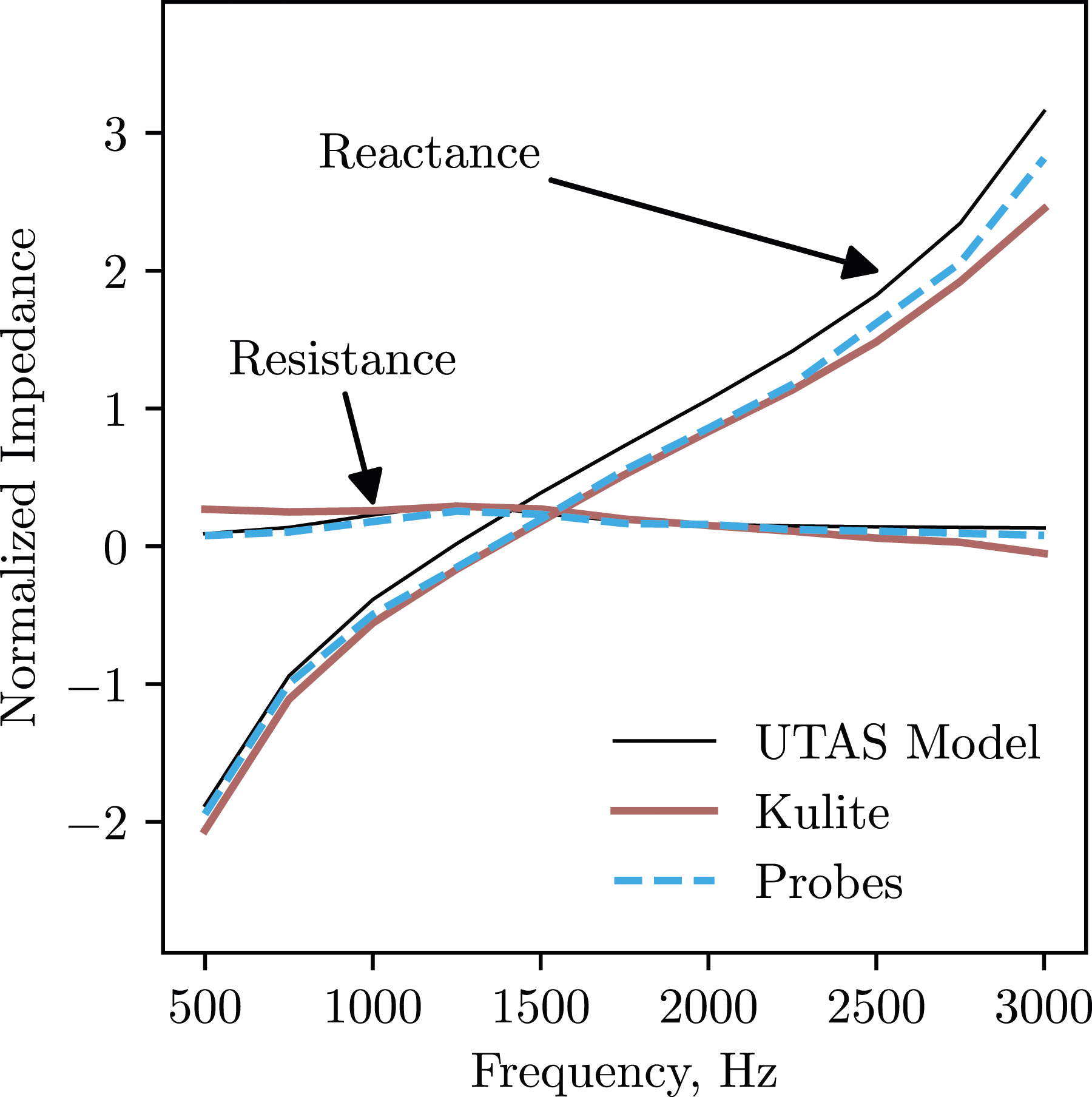

Results obtained with both instrumentation approaches show reasonable agreement with the semi-empirical predictive model, especially the resistance obtained with the capillary probes. However, the discrepancy observed in the reactance at lower frequencies is greater then expected. This discrepancy may occur due to sealing problems or other phenomena arising from the instrumentation. In fact, both instrumentation implies in a reduction of the instrumented cell volume and in an increase of the acoustic velocity at the facesheet. A correction to those effects was reported by Ferrante et al.⁸ and it is given by

z_{corrected} = \frac{z_{meas}}{1 - ε_{w} - ε_{m}} + i \frac{ε_{m}}{\tan (k h)},

(20)

where z_meas is the measured impedance obtained from equation (1); ɛ_w is the ratio of half the cross area of the surrounding cell walls and the area of the liner cell and; ɛ_m is the ratio of the blocked volume due to instrumentation and the cell volume. It is possible to observe in equation (20) that the blocked volume correction is applied on the entire acoustic impedance, although part of the reactance is related to the backplate reflections which depend only on the cavity height. In this sense, an alternate procedure is proposed to apply the correction. The cavity impedance, given by −i cot (kh), is first subtracted from the measured impedance, such that the remaining impedance is related to the facesheet. Then, the corrections are applied, and the cavity impedance is introduced again, which can be written as

z_{corrected, alt .} = \frac{z_{meas} + i \cot (k h)}{1 - ε_{w} - ε_{m}} + i \frac{ε_{m}}{\tan (k h)} - i \cot (k h) .

(21)

One may notice that the acoustic resistance obtained with both methods to correct the impedance is the same. The results obtained with both instrumentation and considering the original correction from Ferrante el al.⁸ and the procedure proposed on this paper are presented in Figure 8(a) and (b), respectively.

Figure 8.

Comparison of measured impedance using the in situ technique and different instrumentation. No flow case, corrections applied to compensate the instrumentation effect. Results for facesheet SPL of 130 dB and upstream acoustic source. (a) Correction from Ferrante et al.⁸ (b) Alternative correction procedure.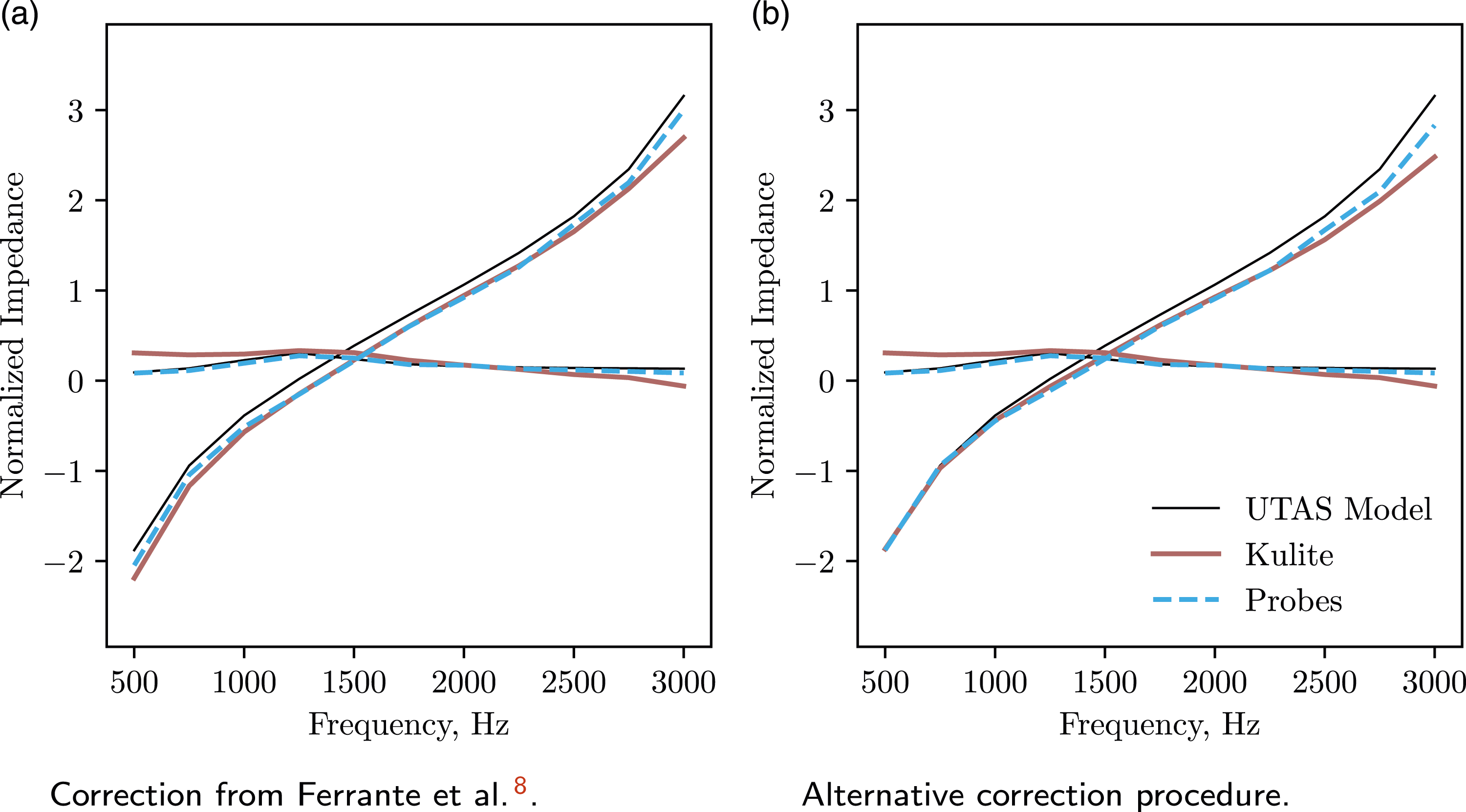

For both correction procedures, the results obtained with the capillary probes present better agreement with the predicted impedance, specially the resistance. Comparing the corrections, improved agreement is obtained for the acoustic reactance when the novel procedure is used. This can be explained by the increase in the reactance amplitude that occurs due to correcting the cavity impedance when equation (20) is applied.

Results with grazing flow

The results obtained with both the Kulite and the probe instrumentation with grazing flow with an average Mach number of 0.3, with no correction applied to the data, with the correction from Ferrant et al.⁸ and the novel procedure proposed, are presented in Figure 9(a)–(c), respectively. Good agreement is observed with the probe instrumentation, especially for the reactance, when using the novel correction procedure. The results obtained with the Kulite method show good agreement in terms of expected reactance, however the resistance does not follow the expected trend.

Figure 9.

Comparison of measured impedance using the in situ technique and differing instrumentation. Average mach number of 0.3, corrections applied to compensate the instrumentation effect. Results for facesheet SPL of 130 dB and upstream acoustic source. (a) No correction applied. (b) Correction from Ferrante et al.⁸ (c) Alternate correction procedure.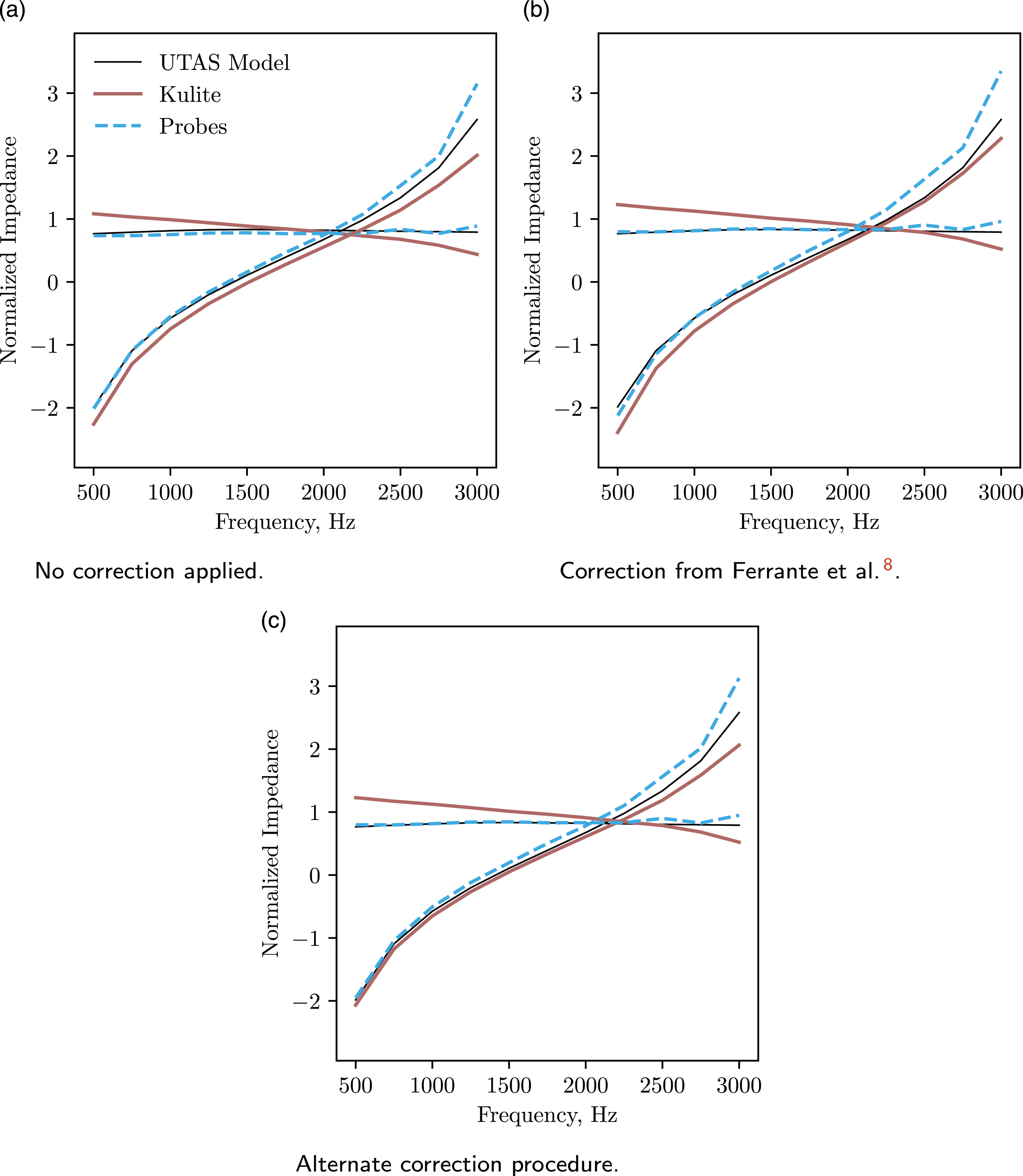

The semi-empirical model used in this work is highly sensitive to the boundary layer discplacement thickness (BLDT).²⁵ In this work, the BLDT used to compute the UTAS model was estimated using the flow profile fitted in a previous study, Spillere et al.¹³

Considering the better agreement observed, the greater stability and ease of operation, from now on in this work only the capillary-probe tube instrumentation is going to be used. Also, the novel correction procedure (equation (21)) is going to be used to compensate the instrumentation effect on measured impedance.

Results and discussion

In this section, the main results obtained for this work are presented. A discussion regarding how the different operational condition affects the experimental evaluated impedance by each method is carried, specially regarding the SPL, which definition may vary from one method to another.

No-flow results

Figure 10 presents the results obtained for 130 dB by means of all three methods considered in this work for both test samples. Good agreement is observed between the three methods, although the resistance curves present a slope at lower frequencies for the eduction techniques, as opposed to the more flat curve from in situ results. This slope is commonly observed with eduction techniques.^4,9

Figure 10.

Results obtained for both samples with all three methods. No-flow condition and 130 dB at the facesheet probe. (a) Sample A. (b) Sample B.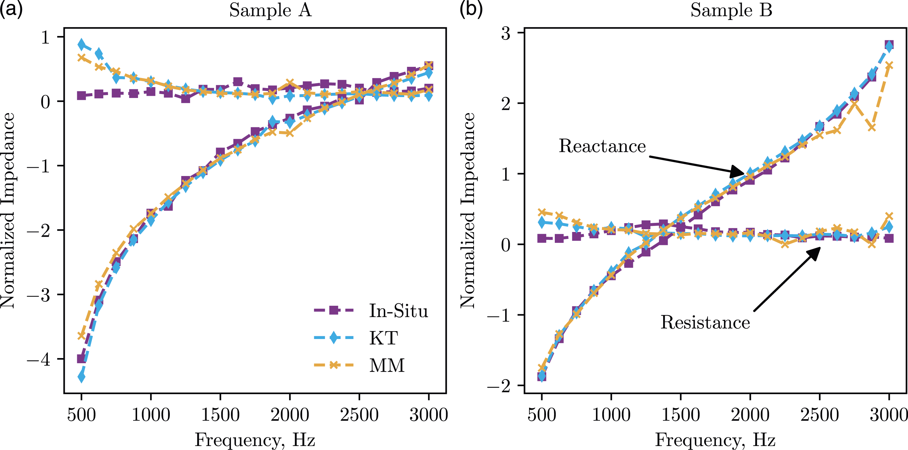

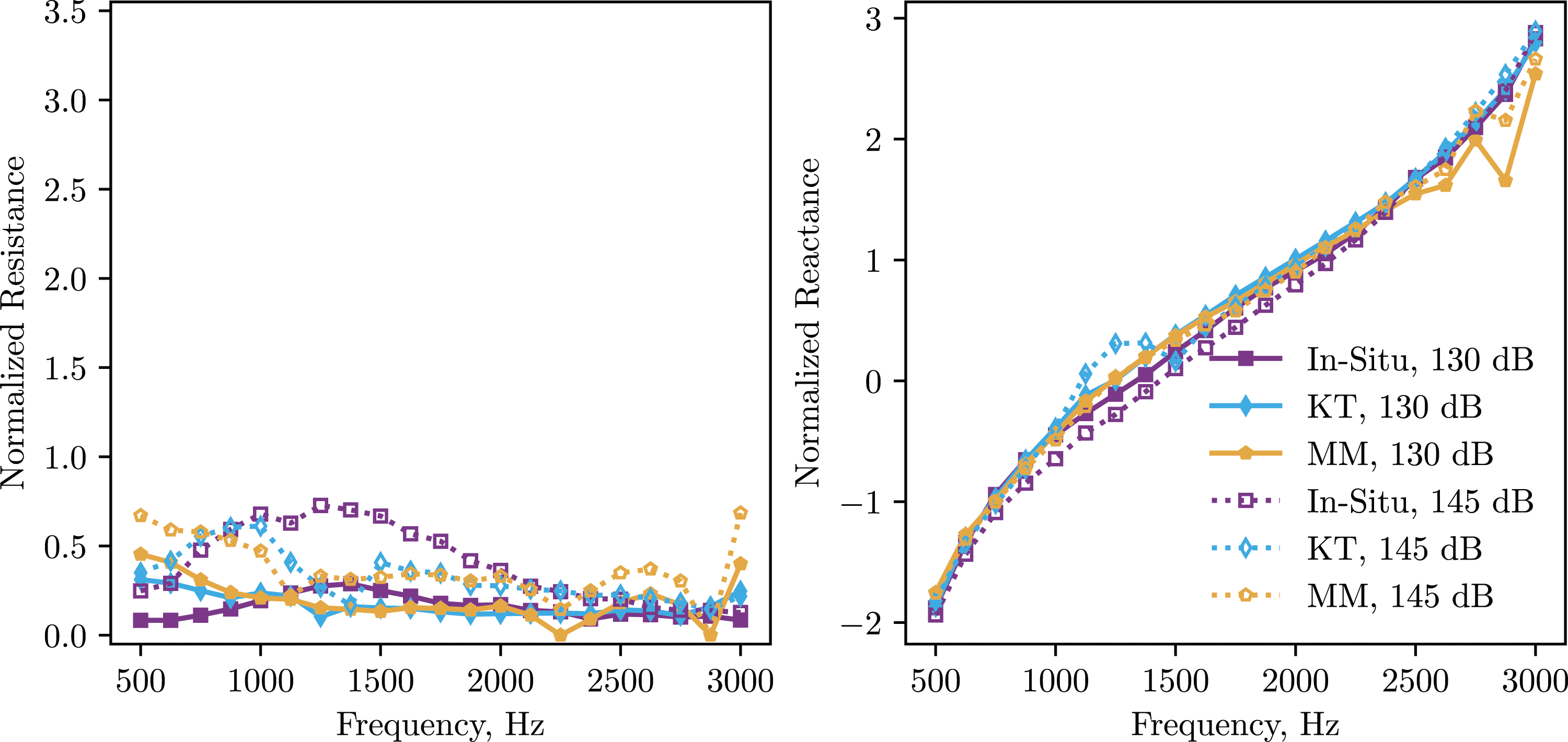
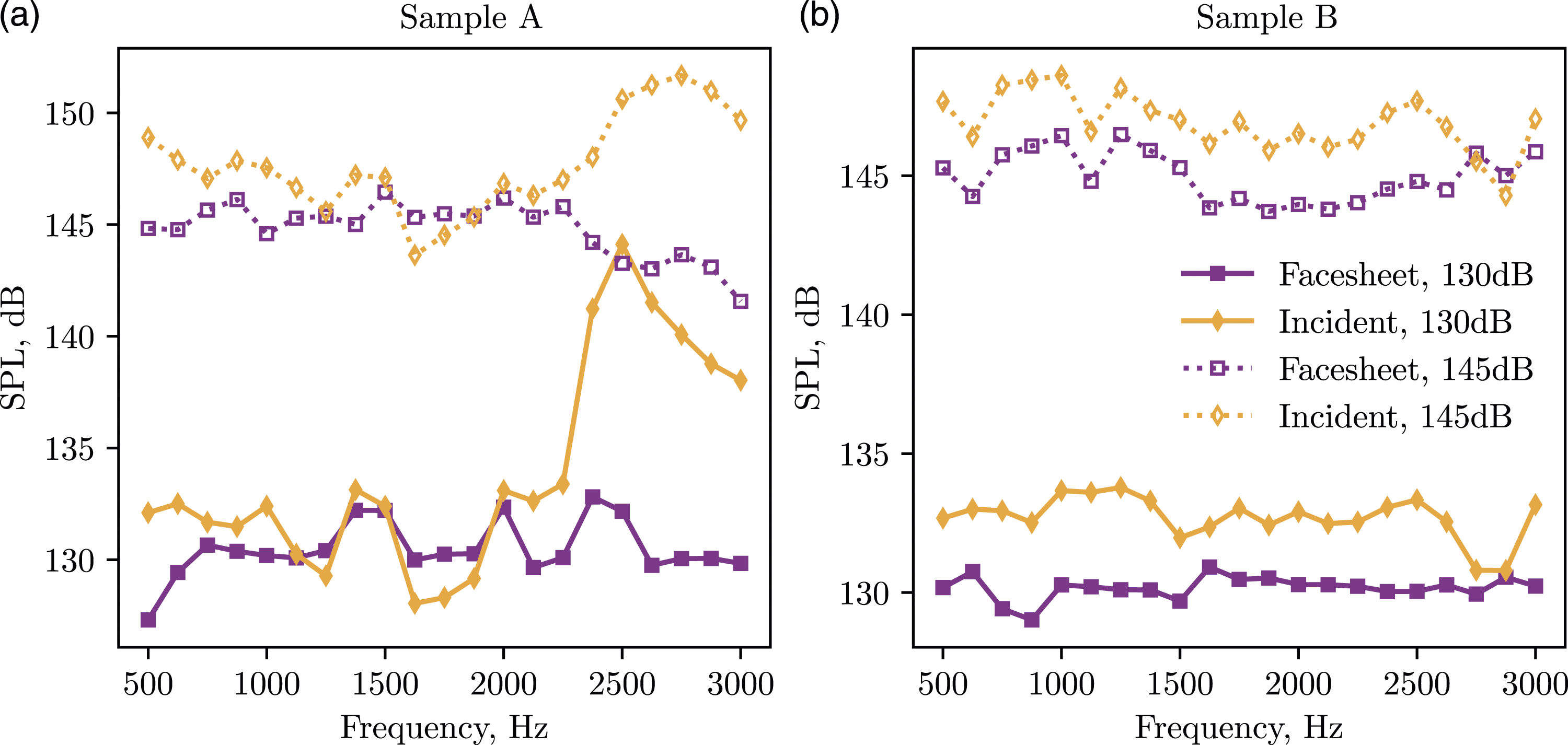
The increase in SPL is expected to induce an increase in the liner resistance due to higher non-linear effects on the perforated facesheet. Also, this non-linear component is expected to reduce as the percentage of open area gets higher.¹ The results obtained for the different methods, with 130 and 145 dB at the facesheet for Sample A and Sample B are presented in Figures 11 and 12, respectively, for no-flow conditions. Figure 13 presents the SPL of the incident plane wave propagating toward the liner, obtained by means of plane wave decomposition, and the SPL at the facesheet probe.

Figure 11.

Results obtained for sample A with all three methods, no-flow condition and different SPL.

Figure 12.

Results obtained for sample B with all three methods, no-flow condition and different SPL.

Figure 13.

SPL of incident plane wave and at the facesheet probe for both samples for the no-flow condition. (a) Sample A. (b) Sample B.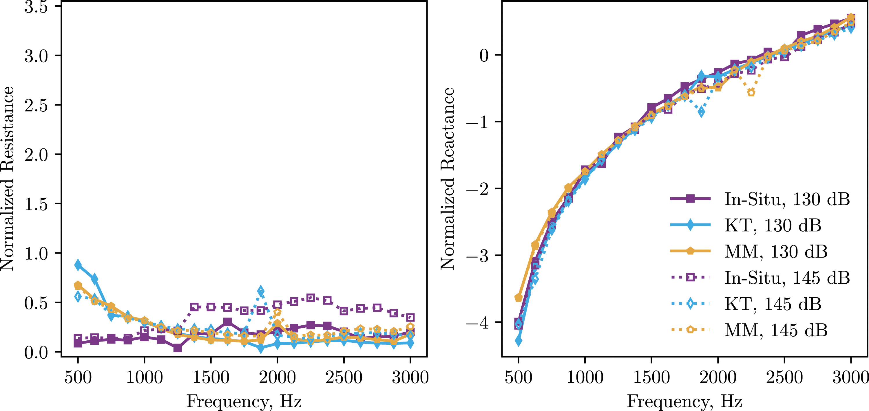

The trends observed with the in situ results when comparing 130 and 145 dB at the facesheet follow those reported in the literature, which is an increase in resistance and an associated decrease in reactance close to the resonance (for instance, see results in Ferrante et al.⁸). These shifts can be explained by the higher acoustic velocity at those frequencies.¹

One may notice that the high SPL effect is more noticeable for the in situ results. This is because a local impedance is obtained when performing the in situ technique. Moreover, the eduction techniques evaluates an average impedance for the whole sample length, and since the acoustic field is attenuated along the liner, the resistance is expected to be lower. The results for the Sample B with the KT algorithm illustrate this. Although good agreement between the KT algorithm results and the in situ method is observed for Sample B with 145 dB, close to the resonance frequency the resistance obtained with the KT algorithm drops. This drop can be explained by the fact that the SPL along the liner sample decreases quickly due to liner attenuation close to the resonance, so the average resistance educed is lower than that obtained with the in situ method.²⁶ The SPL for the microphones used for the KT algorithm during the Sample B measurements with 145 dB are presented in Figure 14. One alternative to address this decay along the axis is to consider an impedance model embedded within the eduction technique, so the impedance spatial variation may be considered, similar as has been applied recently by Roncen et al.²⁷

Figure 14.

SPL at microphones opposite to the wall. Sample B, no-flow condition and 145°dB at liner facesheet.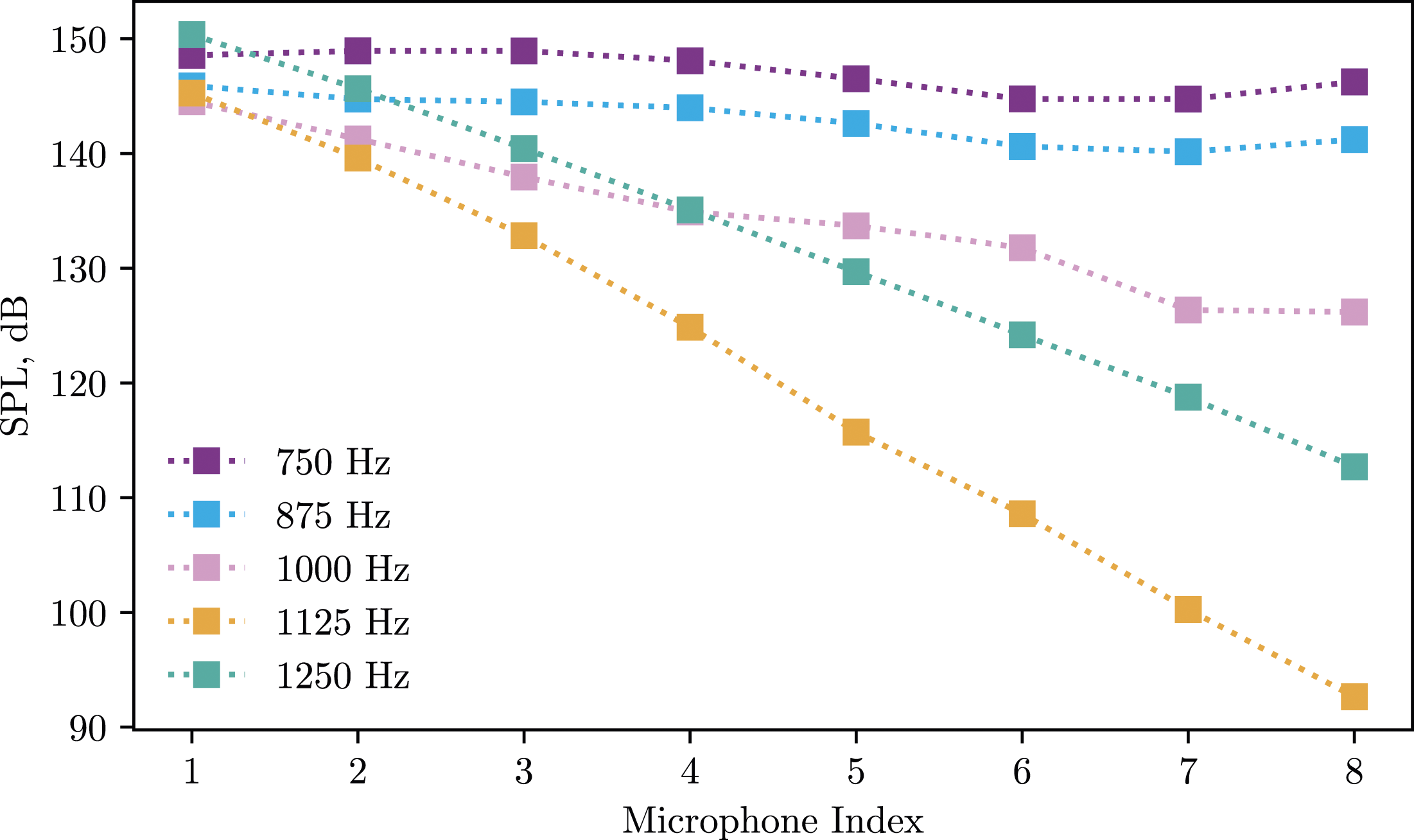

Other phenomena related to the SPL is observed in the Sample A results. The acoustic sources were not capable of reaching the target 145 dB at the facesheet at higher frequencies, although the incident SPL increased considerably. This occurs due to that close to the liner resonance, especially for Sample A, the maximum SPL attained at the cell surface is reduced given the increased absorption around the resonance frequency of approximately 2500 Hz.¹

Results with grazing flow

Figures 15 and 16 show the results obtained for Sample B, with average Mach numbers of 0.3 and 0.5, respectively. The results are presented for both upstream and downstream acoustic source conditions, and for both 130 and 145 dB SPL at the facesheet.

Figure 15.

Results obtained for sample B with average mach number of 0.3, with both upstream (US) and downstream (DS) sources. (a) 130 dB. (b) 145 dB.

Figure 16.

Results obtained for sample B with average mach number of 0.5, with both upstream (US) and downstream (DS) sources. (a) 130 dB. (b) 145 dB.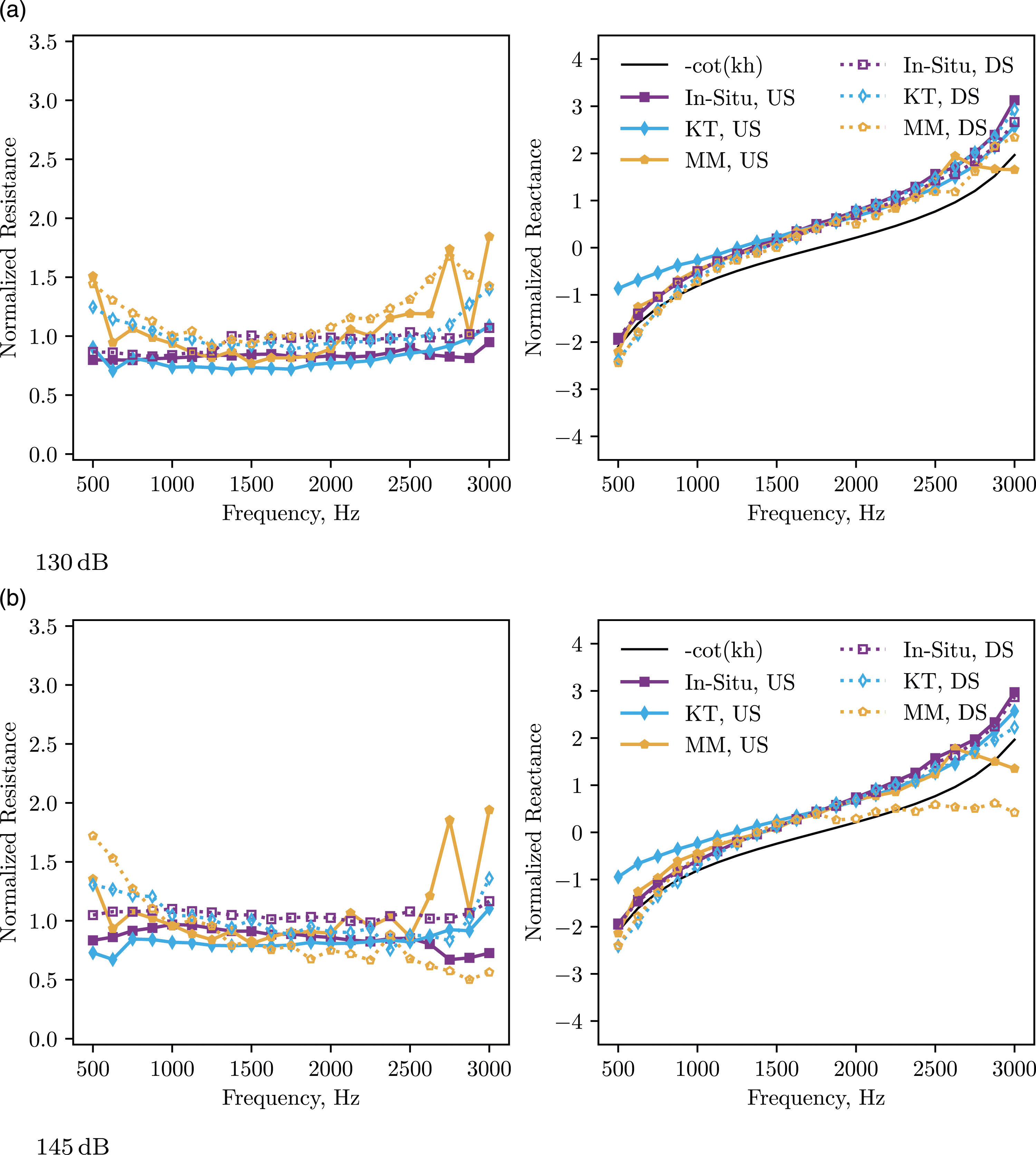

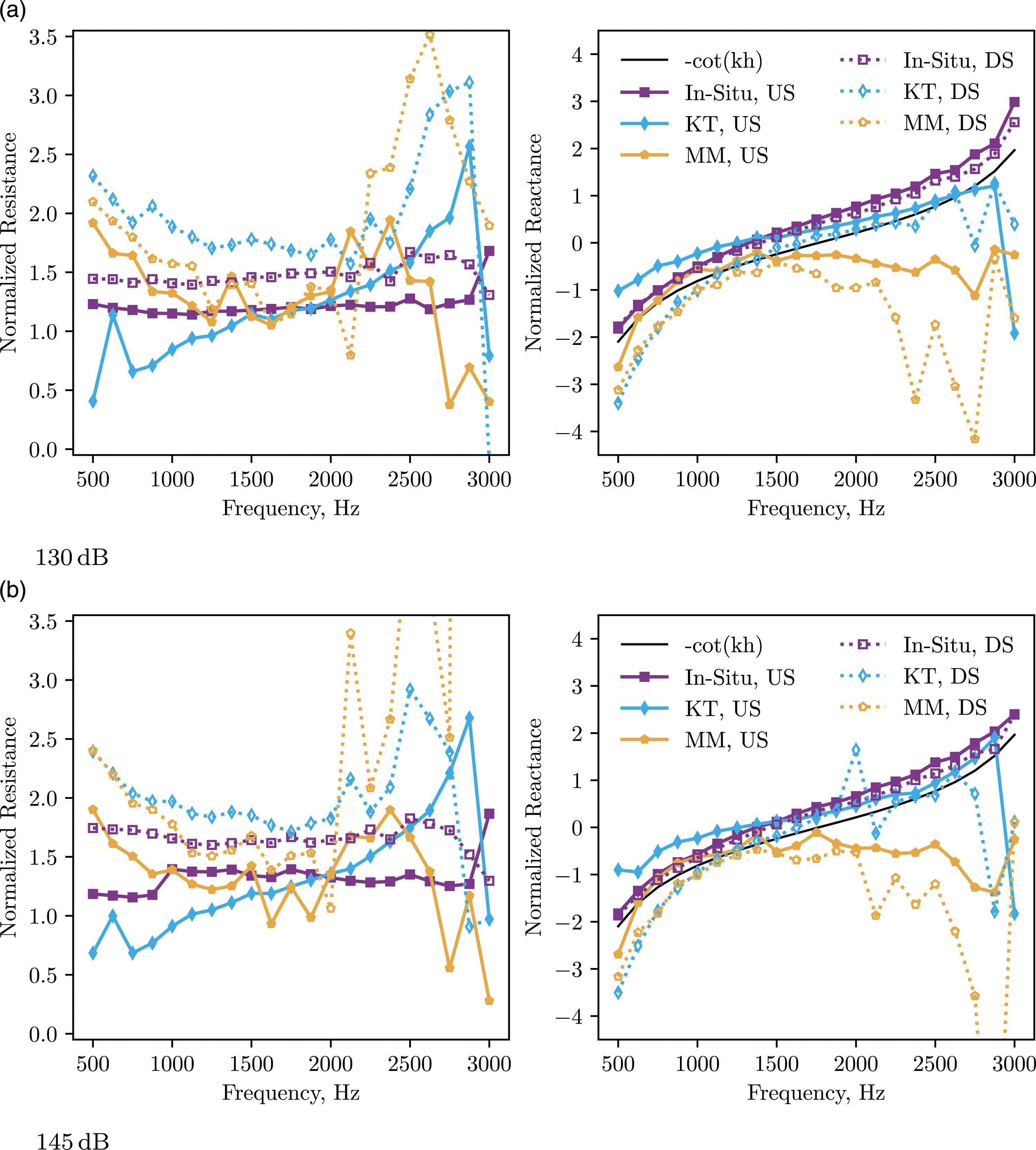
The results obtained for Sample B show good agreement for the reactance, except for the lower frequencies with an upstream source and the KT algorithm and the higher frequencies for the inverse eduction technique, especially with M = 0.5. However, the trend observed at lower frequencies with the KT algorithm follows the behaviour noticed in the documented discrepancies observed between upstream and downstream propagation.^4,19 The higher discrepancies observed with the impedance eduction based on the Mode Matching Method for a mach number of 0.5 may be explained by the longer acoustic propagation distances considered, which may increase the phase mismatch due to the uniform flow hypothesis in both the lined and rigid test sections.

The resistances educed for Sample B with both eduction techniques follows the trends reported for the discrepancy observed for upstream and downstream sources,^4,19 although they do not present good agreement with the other methods. The resistances evaluated via the in situ technique also presents a difference with propagation direction. In this case, the observed trend is for a higher resistance with a downstream source. An hypothesis that can explain these higher resistances is that the flow propagation direction affects the boundary layer refraction,²⁸ therefore the effective impedance of the instrumented cell may vary with the acoustic source position.

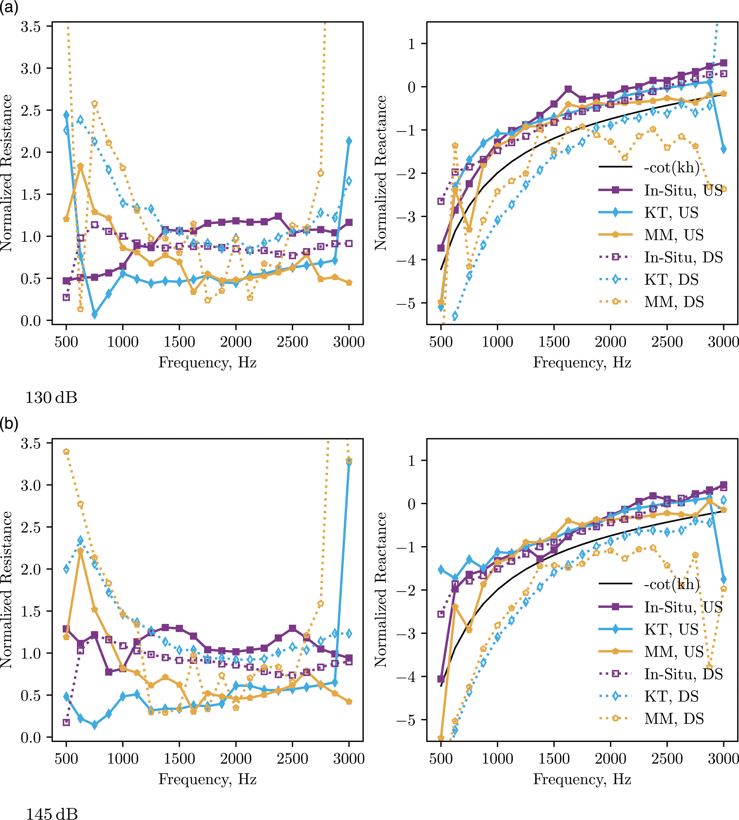
The results obtained for Sample A with average Mach numbers of 0.3 and 0.5 are presented in Figures 17 and 18, respectively. The resistances obtained with the eduction techniques showed improved agreement for this sample, especially with M = 0.3. This can be explained by the higher attenuation of this sample compared to sample B, which implies lower uncertainty levels.²⁹ Good agreement is also observed between the reactances obtained with the in situ and eduction approaches with an upstream acoustic source. Also, one may notice that the trend observed for the difference with propagation direction is the reverse from the noticed for Sample B, so for Sample A is observed a higher resistance with an upstream source. Recent findings obtained with numerical high-fidelity simulations suggests that the in situ technique is strongly affected by the facesheet instrumentation location, even within a single cavity.³⁰ This complex behaviour may be the source of this inconsistent trend between upstream and downstream propagation on the two samples. This phenomena is still not fully comprehended and future work is suggested on this problem.

Figure 17.

Results obtained for sample A with average mach number of 0.3, with both upstream (US) and downstream (DS) sources. (a) 130 dB. (b) 145 dB.

Figure 18.

Results obtained for sample A with average mach number of 0.5, with both upstream (US) and downstream (DS) sources. (a) 130 dB. (b) 145 dB.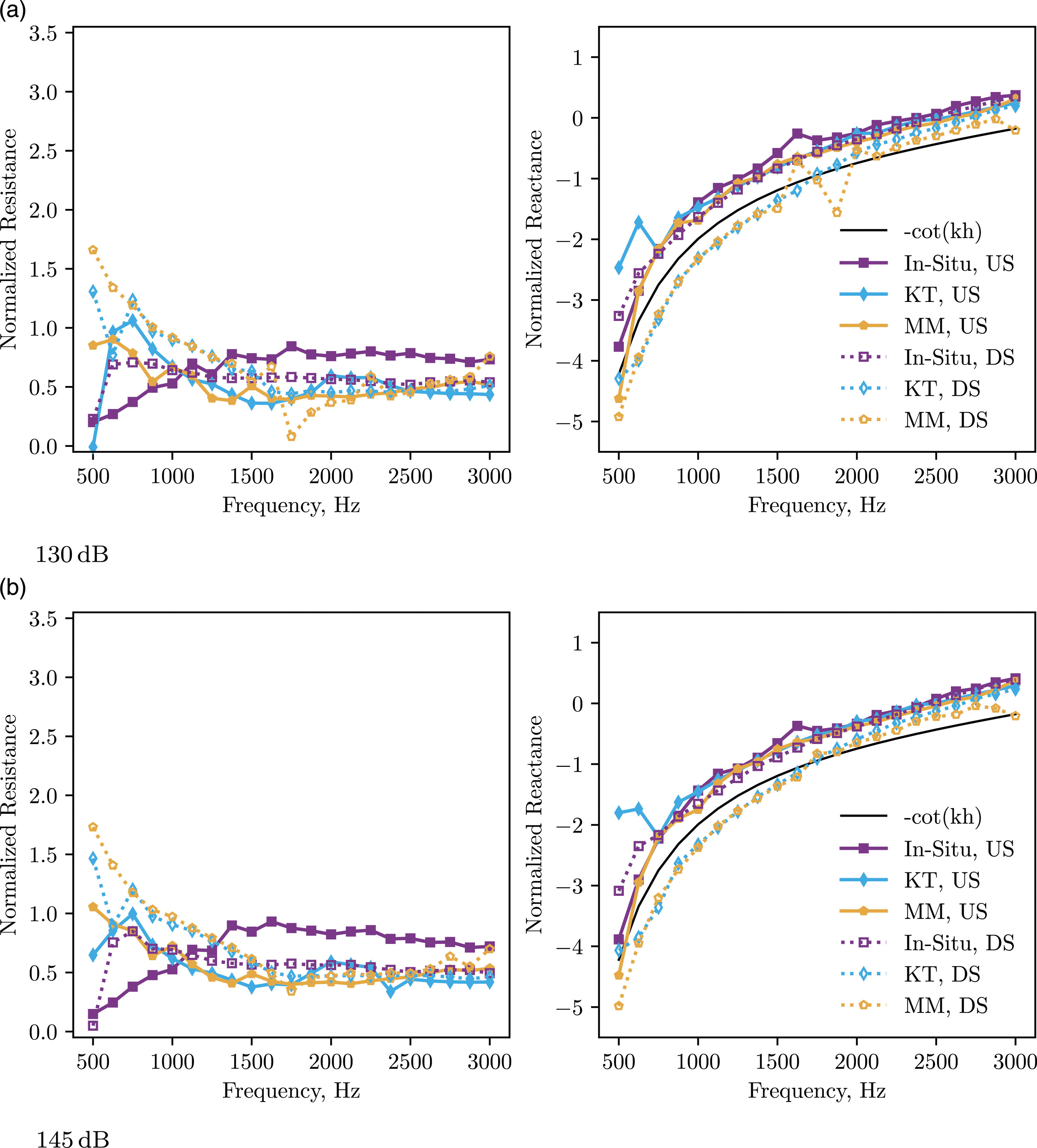

Conclusions

In this work, three experimental techniques to measure the acoustic impedance of liners with grazing flow were compared. The in situ technique, that allows local impedance measurement, and two eduction techniques, one inverse, based on the Mode Matching Method, and one direct eduction, based on the wavenumber extraction by means of the KT algorithm, were considered. The three methods were applied to two typical liner samples, using the UFSC Test Rig facilities, which allowed the measurements to be performed for all methods in one take.

A discussion regarding the in situ sample instrumentation is carried out. Two different instrumentation, one based on miniature microphones and other on capillary-probe tubes are considered, and the results obtained were compared with a predictive model, that was tuned with in situ results. The probe-based instrumentation presented better agreement with expected results, mainly due to the better sealing achieved. Also, a new method to compensate the instrumentation effect on the measured impedance with the in situ technique has been proposed and validated.

Good agreement was found between the three methods in absence of flow and low SPL at the facesheet. For high SPL, the non-linear effect is more noticed in the in situ results, since the eduction methods evaluate an average impedance along the liner sample, so the sound attenuation induces a lower resistance as a result for these methods.

In the cases involving grazing flow conditions, it is hard to draw a single conclusion from the results. The difference between upstream and downstream results is more noticeable between eduction methods, although still present in the results from the in situ technique. Increasing the Mach number and the SPL usually leads to a higher dispersion of the results for all methods, but the in situ results seem to be less affected. Nevertheless, the discrepancies between upstream and downstream results are even larger at higher Mach number and SPL. This highlights the importance of further investigation of liner physics with grazing flow.

In this work, fundamental differences between the results obtained with the in situ technique and traditional eduction methods are highlighted. However, further explanations are required to fully understand the differences observed, especially with flow. Recent findings with high-fidelity numerical simulations³⁰ suggest that the in situ technique is strongly affected by the microphone positioning regarding the surrounding perforate sheet holes. This phenomenon seems to present a strong correlation with fluid-dynamics and acoustics interactions happening in the holes and can lead to complex patterns in higher open-area SDOF, as in the liner Sample A used in this work. Therefore, a detailed study regarding the probe positioning is suggested for future works.

Footnotes

Acknowledgements

The authors acknowledge Jose Alonso-Miralles from Collins Aerospace for supplying the liner samples used in this study and the valuable discussions in the early stages of this work.

Declaration of conflicting interests

The author(s) declared no potential conflicts of interest with respect to the research, authorship, and/or publication of this article.

Funding

The author(s) disclosed receipt of the following financial support for the research, authorship, and/or publication of this article: On behalf of LAB, NTQ, AMNS and JAC, this research was funded by CNPq (National Council for Scientific and Technological Development), FINEP (Funding Authority for Studies and Projects) and EMBRAER S.A.. LAB. acknowledges that this study was also financed in part by the Coordenação de Aperfeiçoamento de Pessoal de Nível Superior – Brasil (CAPES), Finance Code 001.

ORCID iDs

Lucas A Bonomo

André M N Spillere

Julio A Cordioli

Note

References

Murray

Astley

. Development of a single degree of freedom perforate impedance model under grazing flow and high SPL. In: 18th AIAA/CEAS aeroacoustics conference, Colorado Springs, CO, 4–6 June 2012. American Institute of Aeronautics and Astronautics. DOI: 10.2514/6.2012-2294.

Dean

. An in situ method of wall acoustic impedance measurement in flow ducts. J Sound Vib 1974; 34(1): 97–130. DOI: 10.1016/S0022-460X(74)80357-3.

Watson

Jones

. New numerical procedure for impedance eduction in ducts containing mean flow. AIAA J 2011; 49(10): 2109–2122. DOI: 10.2514/1.J050317.

Boden

Cordioli

Spillere

, et al. Comparison of the effect of flow direction on liner impedance using different measurement methods. In: 23rd AIAA/CEAS aeroacoustics conference, Denver, CO, 2 June 2017. American Institute of Aeronautics and Astronautics. DOI: 10.2514/6.2017-3184.

Spillere

Medeiros

Cordioli

. An improved impedance eduction technique based on impedance models and the mode matching method. Appl Acoust 2018; 129: 322–334. DOI: 10.1016/j.apacoust.2017.08.014.

Roncen

Piot

Méry

, et al. Wavenumber-based impedance eduction with a shear grazing flow. AIAA J 2020; 58(7): 3040–3050. DOI: 10.2514/1.J059100.

Watson

Carpenter

Jones

. Performance of Kumaresan and Tufts algorithm in liner impedance eduction with flow. AIAA J 2015; 53(4): 1091–1102. DOI: 10.2514/1.j053705.

Ferrante

De Roeck

Desmet

, et al. Back-to-back comparison of impedance measurement techniques applied to the characterization of aero-engine nacelle acoustic liners. Appl Acoust 2016; 105: 129–142. DOI: 10.1016/j.apacoust.2015.12.004.

Serrano

Spillere

Cordioli

, et al. Comparisons between eduction and in-situ measurement procedures for aero engine liner impedance. In: 23rd AIAA/CEAS aeroacoustics conference, Denver, CO, 2 June 2017. American Institute of Aeronautics and Astronautics. DOI: 10.2514/6.2017-3024.

10.

Kumaresan

Tufts

. Estimating the parameters of exponentially damped sinusoids and pole-zero modeling in noise. IEEE Trans Acoust 1982; 30(6): 833–840. DOI: 10.1109/TASSP.1982.1163974.

11.

Ingard

. Influence of fluid motion past a plane boundary on sound reflection, absorption, and transmission. J Acoust Soc Am 1959; 31: 1035–1036. DOI: 10.1121/1.1907805.

12.

Myers

. On the acoustic boundary condition in the presence of flow. J Sound Vib 1980; 71: 429–434. DOI: 10.1016/0022-460X(80)90424-1.

13.

Spillere

AMN

Bonomo

Cordioli

, et al. Experimentally testing impedance boundary conditions for acoustic liners with flow: beyond upstream and downstream. J Sound Vib 2020; 489: 115676. DOI: 10.1016/j.jsv.2020.115676.

14.

Boyd

. Chebyshev and fourier spectral methods. 2nd ed. Mineola, NY: Dover Books on Mathematics, Dover Publications, 2001.

15.

Gabard

Astley

. A computational mode-matching approach for sound propagation in three-dimensional ducts with flow. J Sound Vib 2008; 315(4): 1103–1124. DOI: 10.1016/j.jsv.2008.02.015.

16.

Levenberg

. A method for the solution of certain non-linear problems in least squares. Q Appl Math 1944; 2(2): 164–168. DOI: 10.1090/qam/10666.

17.

Marquardt

. An algorithm for least-squares estimation of nonlinear parameters. J Soc Ind Appl Math 1963; 11(2): 431–441. DOI: 10.1137/0111030.

18.

Dokumaci

. Sound transmission in narrow pipes with superimposed uniform mean flow and acoustic modelling of automobile catalytic converters. J Sound Vib 1995; 182(5): 799–808. DOI: 10.1006/jsvi.1995.0233.

19.

Renou

Aurégan

. Failure of the ingard–myers boundary condition for a lined duct: an experimental investigation. J Acoust Soc Am 2011; 130(1): 52–60. DOI: 10.1121/1.3586789.

20.

Weng

Schulz

Ronneberger

, et al. Flow and viscous effects on impedance eduction. AIAA J 2018; 56(3): 1118–1132. DOI: 10.2514/1.J055838.

21.

Krishnappa

. Cross-spectral method of measuring acoustic intensity by correcting phase and gain mismatch errors by microphone calibration. J Acoust Soc Am 1981; 69: 307–310. DOI: 10.1121/1.385314.

22.

International Organization for Standardization . ISO 3966:2008 - measurement of fluid flow in closed conduits — velocity area method using pitot static tubes. Geneva, Switzerland: International Organization for Standardization, 2008.

23.

Shin

Hammond

. Fundamentals of signal processing for sound and vibration engineers. Hoboken, NJ: John Wiley & Sons, 2008.

24.

Guess

. Calculation of perforated plate liner parameters from specified acoustic resistance and reactance. J Sound Vib 1975; 40: 119–137. DOI: 10.1016/S0022-460X(75)80234-3.

25.

Ruiz

Kwan

. Validation of goodrich perforate liner impedance model using nasa langley test data. In 14th AIAA/CEAS aeroacoustics conference (29th AIAA aeroacoustics conference), Vancouver, BC, 6 May 2008. DOI: 10.2514/6.2008-2930.

26.

Chen

. On spatially varying acoustic impedance due to high sound intensity decay in a lined duct. J Sound Vib 2020; 483: 115430.

27.

Roncen

Méry

Piot

, et al. Spatially-varying impedance model for locally reacting acoustic liners at a high sound intensity. J Sound Vib 2022; 524: 116741. DOI: 10.1016/j.jsv.2021.116741.

28.

Spillere

Braga

Seki

, et al. Design of a single degree of freedom acoustic liner for a fan noise test rig. Int J Aeroacoustics 2021; 20: 708–736. DOI: 10.1177/1475472X211023831.

29.

Bonomo

Spillere

AMN

Cordioli

. Parametric uncertainty analysis for impedance eduction based on prony’s method. AIAA J 2020; 58: 3625–3638. DOI: 10.2514/1.j059071.

30.

Pereira

Bonomo

Quintino

, et al. Validation of high-fidelity numerical simulations of acoustic liners under grazing flow. In: AIAA AVIATION 2023 Forum, San Diego, CA, 12–16 June 2023. American Institute of Aeronautics and Astronautics. DOI: 10.2514/6.2023-3503.

A comparison of in situ and impedance eduction experimental techniques for acoustic liners with grazing flow and high sound pressure level

Abstract

Keywords

Introduction

Experimental techniques

In situ technique

Impedance eduction

Governing equations

Mode-matching method

Inverse eduction procedure

Direct eduction procedure - KT algorithm

Experimental setup

UFSC liner test rig

Test samples

Test conditions

In situ instrumentation analysis

Calibration procedure and sample preparation

No-flow results

Results with grazing flow

Results and discussion

No-flow results

Results with grazing flow

Conclusions

Footnotes

Acknowledgements

Declaration of conflicting interests

Funding

ORCID iDs

Note

References