
Abstract
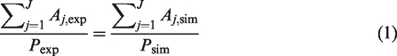
Most acoustic imaging methods assume the presence of point sound sources and, hence, may fail to correctly estimate the sound emissions of distributed sound sources, such as trailing-edge noise. In this contribution, three integration techniques are suggested to overcome this issue based on models considering a single point source, a line source, and several line sources, respectively. Two simulated benchmark cases featuring distributed sound sources are employed to compare the performance of these integration techniques with respect to other well-known acoustic imaging methods. The considered integration methods provide the best performance in retrieving the source levels and require short computation times. In addition, the negative effects of the presence of unwanted noise sources, such as corner sources in wind-tunnel measurements, can be eliminated. A sensitivity analysis shows that the integration technique based on a line source is robust with respect to the choice of the integration area (shape, position, and mesh fineness). This technique is applied to a trailing-edge-noise experiment in an open-jet wind tunnel featuring a NACA 0018 airfoil. The location and far-field noise emissions of the trailing-edge line source were calculated.
Introduction
The use of conventional acoustic beamforming techniques1–4 incorporates the assumption of point sound sources at every scan point of a considered scan grid. In practice the noise sources are often distributed over extended regions, like along the edges of aircraft wings5–9 or wind turbine blades.5,10–18 For these cases, conventional beamforming fails in determining correctly the emitted sound levels, if the peak levels in the source map are considered. To overcome this issue, the source power integration (SPI) technique11,19 was proposed, which sums and scales the results of conventional frequency domain beamforming (CFDBF) over (part of) a scan grid. The idea is to retrieve the source level of a distributed source, i.e. a single value.
A drawback of SPI is the possible contamination by noise sources outside the region of integration (ROI). For example, the region producing airfoil trailing-edge noise, e.g. measured in wind-tunnel experiments, can be heavily contaminated by “corner sources appearing at the junctions of the airfoil and the wind-tunnel walls or end plates.
For better results in the situations given above, extensions of the SPI method
20
can be considered:
By the assumption of the presence of a line source instead of a monopole source (SPIL). SPIL was previously applied to synthetic data of trailing-edge noise in a closed-section wind-tunnel measurement heavily contaminated by background noise, in the framework of the phased-array methods menchmark21–24 (the reader is referred to the Description of the test cases section for a detailed explanation). The objective was the calculation of the spectrum emitted by the line source. The SPIL method provided the best results for this case,
25
compared to other well-known methods, such as CLEAN-SC,26–28 DAMAS,
29
functional beamforming,30–33 covariance matrix fitting (CMF),
34
or orthogonal beamforming.35–37 By the generalization of the SPIL technique to distributed sound sources on multiple ROIs. This method is called Inverse SPI (ISPI) and is introduced in this paper. ISPI is applied to realistic wind-tunnel simulations of trailing-edge noise contaminated by corner sources.
In order to assess the dependence of SPIL on its settings, a sensitivity analysis is performed. With the findings of the sensitivity analysis, SPIL is applied to an illustrative trailing-edge-noise experiment of a NACA 0018 airfoil in an open-jet wind tunnel. The purpose of this experiment was to analyze the performance of porous trailing edges18,38–41 as a noise-reduction measure. This experiment was used since the location of the line source causing trailing-edge noise is expected to vary when porous inserts are used
42
and this parameter can be estimated using the SPIL method.
This paper is structured as follows: The Theory section briefly explains the basics of the SPI, SPIL and ISPI techniques. The simulated and experimental setups employed for the evaluation of these methods are introduced in the Description of the test cases section. The Simulated results section presents the comparison between the results obtained by the aforementioned integration methods, as well as other well-known acoustic imaging methods when using synthetic data. The Sensitivity analysis for SPIL section contains a detailed sensitivity analysis of the SPIL technique with respect to some practical parameters, such as the size and shape of the ROI. Finally, the Experimental results section gathers the main outcomes from the experimental campaign.
Theory
For well-separated monopole sources, CFDBF provides the correct source sound pressure levels
Different integration methods have been proposed 20 to overcome all these issues. Three of them are described below, in increasing order of sophistication.
Source power integration
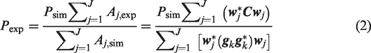
In order to limit the effect of the array's point spread function (PSF), the SPI technique11,19 was proposed. The idea of the SPI method is to integrate the source power within a predefined ROI, and suppose that the integrated source power is represented by a simulated unit monopole. The integrated source power needs to be scaled by determining a certain scaling factor to normalize the total source power to a unit monopole source. This scaling factor therefore represents the total sound power within the ROI.
Figure 1(a) shows an arbitrarily distributed sound source obtained from an experiment. At the jth grid point, the source power estimate is
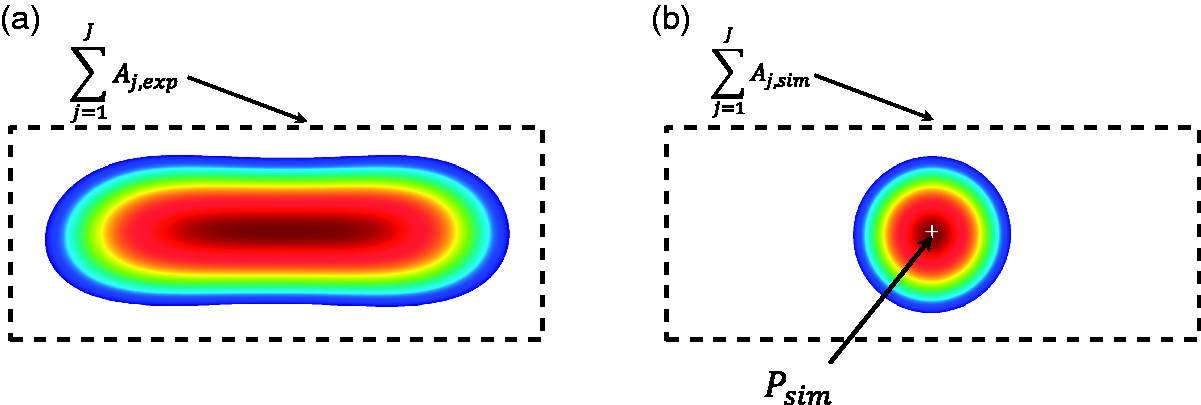
(a) Example of the application of the SPI technique: experimental distributed sound source and (b) simulated point source. The dashed black rectangle denotes the ROI, and the white + marker the location of the simulated point source.
For experimental measurements, the main diagonal of the CSM is usually removed to reduce the influence of noise which is incoherent for all the array microphones.2,26 This process can give a negative source power for some grid points, which is not physically possible. Therefore, the values where
The ROI should encompass the complete sound source (see Figure 1(a)) and be large enough to capture the potential main-lobe broadening due to coherence loss. 43 However, it should be ensured that the variation of the main lobe width is always captured in the ROI for all considered frequencies. Furthermore, the choice of the ROI should also avoid the contributions and sidelobes from other sound sources and the noise floor from the source map. 43
This integration technique has been successfully applied to several wind-tunnel experiments5,10–15,25 and aircraft flyover measurements,9,45,46 yielding accurate sound pressure levels, even in the cases when coherence loss is present. 43 A similar integration technique can be applied to the results obtained with functional beamforming.46,47
Extension to line sources (SPIL)
In aeroacoustic measurements of leading- and/or trailing-edge noise, the presence of a line source can be expected. When a certain source distribution is known beforehand, the simulated monopole source in the SPI method can be replaced by another predefined source distribution to better represent the physical characteristics of the source. In this case, the simulated monopole is replaced by a set of linearly-arranged incoherent monopoles.
In practice, a large number of K simulated incoherent point sources of equal power level are placed along the expected location of the experimental line source with steering vectors

For distributed sound sources, the source coherence should be taken into account. However, the coherence length of a source is typically much smaller than the main lobe width, so the assumption of distributed incoherent monopoles is, in essence, valid. 43
This technique has already been applied to trailing-edge noise measurements in an open-jet 14 and a closed-section wind tunnel14,48 and a closed-section wind tunnel 16 with very satisfactory results.
Inverse SPI
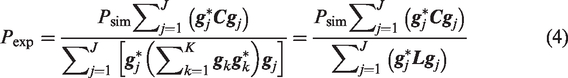
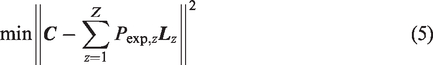
The SPI method can be further extended to include multiple ROIs for which the simulated sources are allowed to differ in power. This is known as inverse SPI (ISPI). It addresses a similar minimization problem as the one presented in equation (3) considering Z different ROIs simultaneously (each of them with different sound powers
This integration technique is especially useful for wind-tunnel measurements featuring mounting plates for the test model, which can cause extraneous noise sources on the junction between the test model and the mounting plates, also known as “corner” sources. 50 These sources can contaminate the results of the ROI of interest in experiments.12–15,51 The aim of the ISPI technique is to exclude their influence on the actual results by defining dedicated ROIs at the expected locations of the “corner” sources.
In the limit of only a single grid point as the ROI, i.e. Z = J, the obtained method is similar to DAMAS. 29
Description of the test cases
Synthetic line-source benchmark
This synthetic case is obtained from the phased-array methods benchmark.21–24 (The acoustic data and more details of this benchmark case (B1) are currently available online in the following website: https://www-fs.tu-cottbus.de/aeroakustik/analytical/) The case consists of recorded microphone array data from a simulated acoustic line source. The measurement data were subject to severe incoherent noise. This representation is typical for measuring trailing-edge noise in a closed-section wind tunnel for which the microphones are flush-mounted in the wall of the tunnel. For recordings in this setup, noise is introduced due to the wall-boundary-layer turbulence. 25
This benchmark case was proposed by Sijtsma (PSA3) 52 and the preliminary results obtained by several researchers using different acoustic imaging methods have been published recently by Sarradj et al. 25
The considered coordinate system is shown in Figure 2, with the x-axis in the streamwise direction, the y-axis perpendicular to the line source and pointing away from the array plane, the z-axis in the spanwise direction of the line source pointing upwards and the center in the middle of the line source.
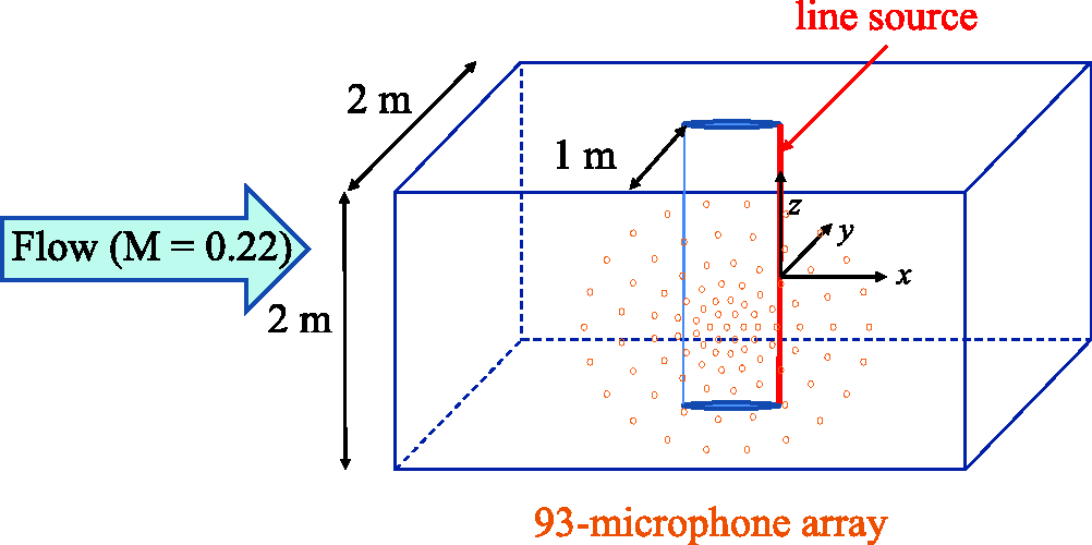
Diagram explaining the computational setup for the line source benchmark case. Adapted from Sarradj et al. 25
The setup for this case can be seen in Figure 2. A 2-m-long line source with short correlation length was simulated between z = −1 m and z = 1 m located at
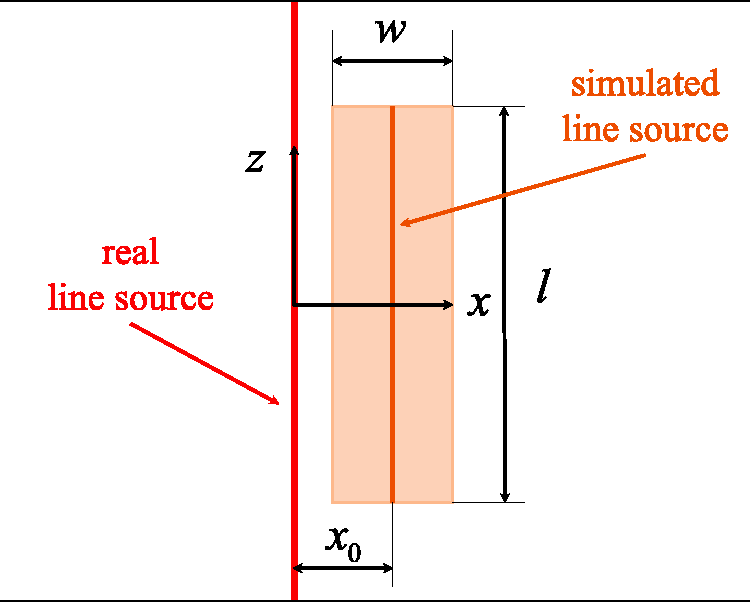
Diagram explaining the parameters that define the ROI (shaded in orange).
A detailed explanation of the signal generation process can be found in Sarradj et al.
25
The line source was synthesized as a large number of incoherent monopoles at equal spacing and equal strengths. This results in a source strength distribution per unit length denoted as

On the top of the signal generated by the line source, Gaussian white noise, incoherent from microphone to microphone, was added with an
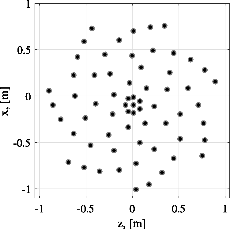
The challenge of this benchmark is to obtain the value of
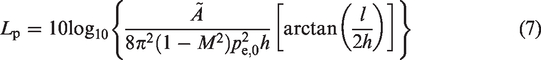
For this case, h = 1 m and l = 2 m, so equation (7) can be simplified to
Synthetic line-source and corner sources
To investigate the merits of ISPI, an additional array simulation was considered. The same microphone array was used as in the previous section. A line source was synthesized at the same position (see Figure 2), and also the same Mach number was used. The source strength distribution
The challenge is to obtain the correct value of
Experimental setup
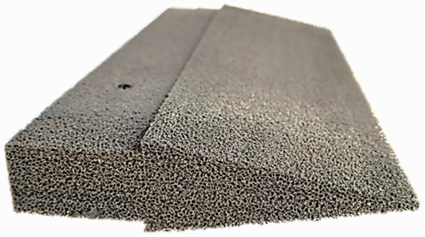
The experiments were performed in the aeroacoustic vertical open-jet wind tunnel (A-Tunnel) at Delft University of Technology. It was verified that across the test section (0.4 m × 0.7 m), the freestream velocity was uniform within 0.5% and the turbulence intensity was below 0.1%. The measurements were performed on a NACA 0018 airfoil with chord
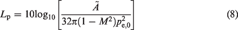
Metal foam trailing-edge insert used in the experiment. The total length of the insert is 0.06 m. Extracted from Carpio et al. 41
The airfoil was installed between two wooden plates of 1.2 m length, to assure the two-dimensionality of the flow,
53
and was located 0.5 m away from the outlet of the wind-tunnel nozzle (see Figure 5(a)). In order to force transition to turbulence, a tripping device consisting of carborundum elements of 0.84 mm nominal size randomly distributed over a tape of 1 cm width, placed at 20% of the chord on both suction and pressure sides and extending the whole span b (following the recommendations in Braslow et al.
54
), was used. The turbulent nature of the boundary layer was assessed using a remote wall-pressure probe. The experiments were performed at a chord-based Reynolds number of
(a) Illustration of the experimental setup in the A-tunnel indicating the coordinate system. (b) Schematic view of the experimental setup and the location of the ROI (shaded in orange) for the trailing-edge noise measurements.
The streamwise vertical coordinate system used in the present manuscript has its origin at the intersection between the trailing edge and the midspan plane of the airfoil, and the x- and z-axes are respectively aligned with the streamwise and spanwise directions, as depicted in Figure 5(a). The y-axis is perpendicular to the xz plane and points towards the microphone array.
A phased microphone array consisting of 64 G.R.A.S. 40PH
55
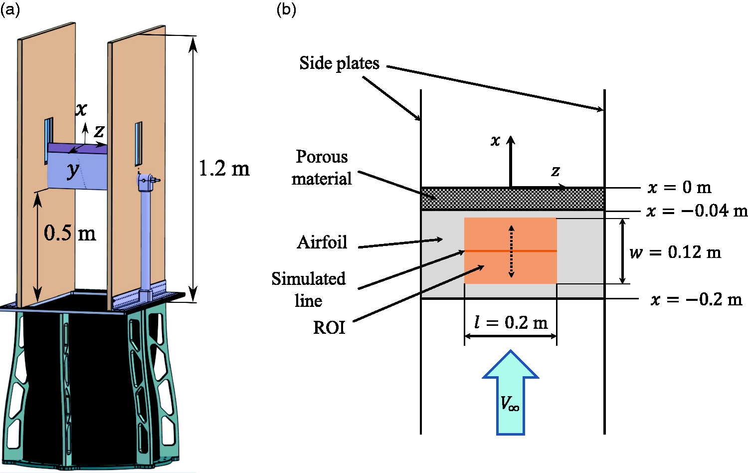
free-field microphones with integrated CCP preamplifiers was employed for recording the far-field noise emissions of the airfoil. These microphones have a flat frequency response range of 10 Hz to 20 kHz within a sensitivity of 50 mV/Pa at 250 Hz. The microphone distribution corresponds to an adapted version of the Underbrink spiral design2,56,57 with seven spiral arms of nine microphones each and an additional microphone located at the center of the array (see Figure 6). The diameter of the array is approximately 2 m and the distance from the array plane to the trailing edge (for an angle of attack
Microphone array distribution for the A-tunnel measurements.
For each measurement a sampling frequency of 50 kHz and 60 s of recording time were used. The acoustic data were averaged in time blocks of 8192 samples (Th = 163.84 ms) and windowed using a Hanning weighting function with 50% data overlap, following Welch's method.
58
With these parameters, the frequency resolution is
For beamforming, a scan grid covering a region ranging from
Results for cases with synthetic data
Synthetic line-source benchmark
A preliminary study of the acoustic data using CFDBF confirmed that removing the main diagonal of the CSM
11
is necessary since the SNR values are very low and the influence of incoherent noise is very strong. The convection of the sound waves due to the flow inside the wind tunnel also needs to be taken into account for obtaining valid results.
11
Four source plot examples for the whole frequency range (50 Hz to 10 kHz) are presented in Figure 7 to illustrate this phenomena. The overall sound pressure levels (
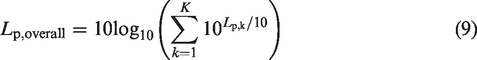
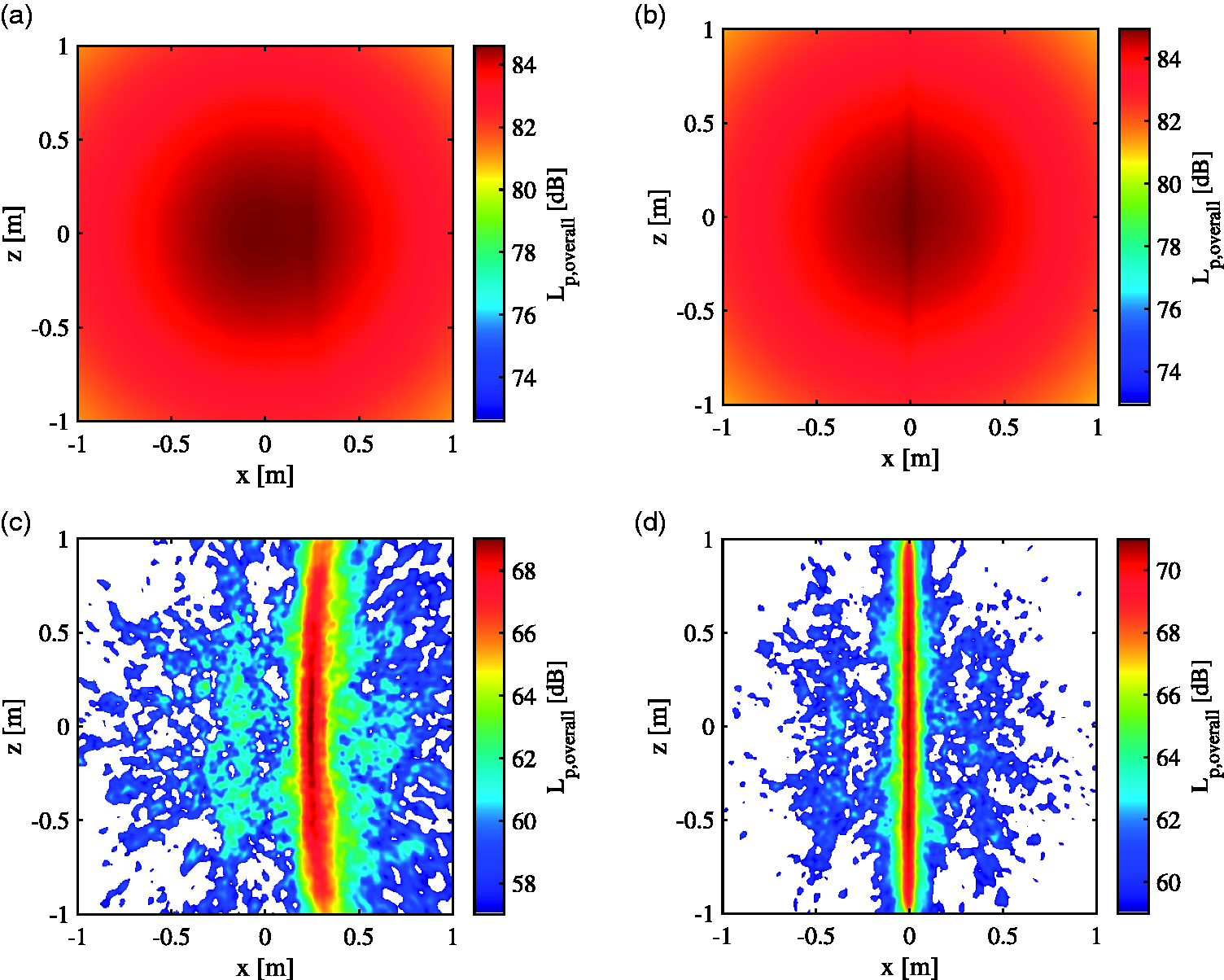
Obtained source maps with CFDBF for the whole frequency range (50 Hz to 10 kHz): (a) without DR or considering convective effects; (b) without DR of the CSM, but considering convective effects; (c) DR without considering convective effects; (d) DR and considering convective effects.
Figure 7(a) shows the beamforming results without applying the diagonal removal (DR) or convective effects; Figure 7(b) includes convective effects but no DR; Figure 7(c) includes DR but no convective effects and Figure 7(d) includes both effects. In Figure 7(a) and (b), the incoherent noise hinders any useful interpretation of the source plot and the presence of the line can barely be detected. Moreover, the
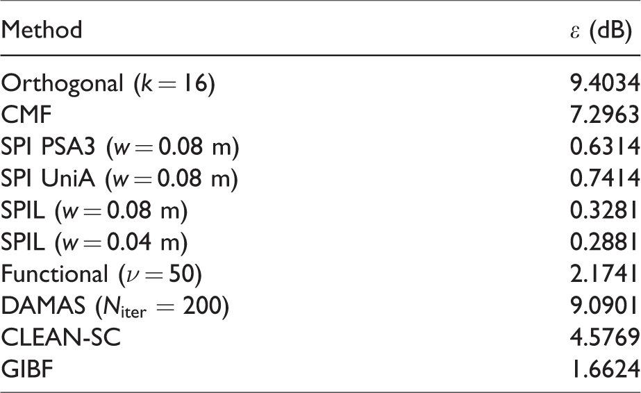
Several well-known acoustic imaging methods 3 (orthogonal beamforming, CMF, functional beamforming, SPI, SPIL, DAMAS, CLEAN-SC, and Generalized Inverse Beamforming (GIBF)) were applied by different researchers using the parameters specified in Table 1. Most of the solutions obtained were extracted from Sarradj et al. 25 Only one solution per method is considered, but significant differences were found when different contributors applied the same method, such as DAMAS or CLEAN-SC, 25 which is not a desired feature.
Overview of the contributors and parameters for each method. Adapted from Sarradj et al. 25
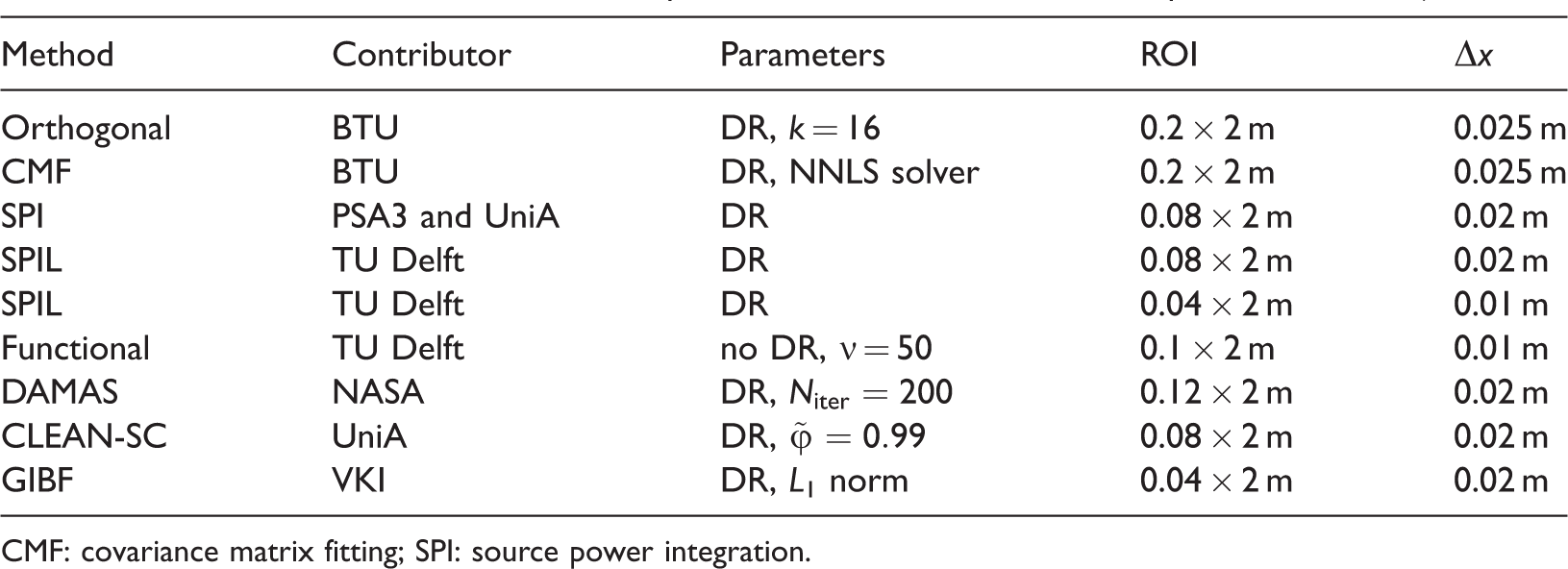
CMF: covariance matrix fitting; SPI: source power integration.
In the second column of Table 1, BTU corresponds to the Brandenburg University of Technology Cottbus-Senftenberg and TU Berlin in Germany, NASA to the NASA Langley Research Center in the United States, PSA3 to Pieter Sijstma Advanced AeroAcoustics in the Netherlands, TU Delft to Delft University of Technology in the Netherlands, and UniA to the University of Adelaide in Australia.
25
In the third column of Table 1, the relevant parameters of each method are specified: k is the number of eigenvalues considered for orthogonal beamforming, ν is the functional beamforming exponent,
The frequency spectra obtained by these methods for the line-source benchmark are presented in Figure 8(a), as well as the exact solution given by equation (6). The relative errors made by each method with respect to the exact solution,
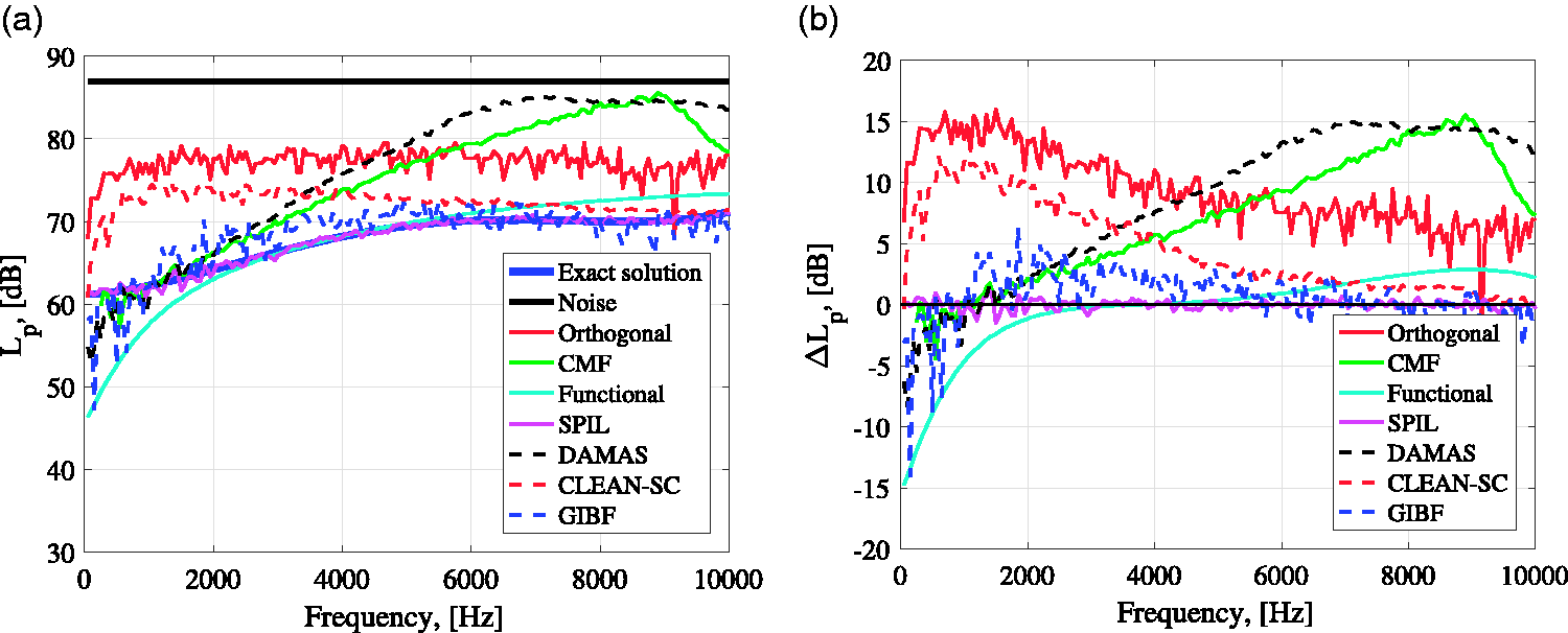
(a) Results of the line-source benchmark for different acoustic imaging methods. Adapted from Sarradj et al.
25
(b) Relative errors
Average absolute errors made by each method with respect to the exact solution.
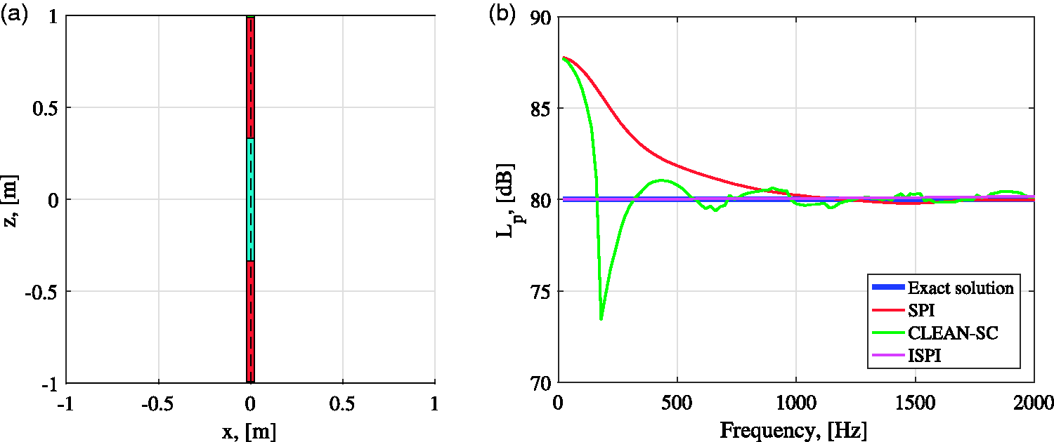
For clarity reasons, the solutions obtained by UniA and PSA3 using the SPI method were not included in Figure 8 but instead, a separate study is presented in Figure 9 comparing the performance of SPI and SPIL. In order to have a fair comparison all the ROI parameters were kept constant: w = 0.08 m, l = 2 m,
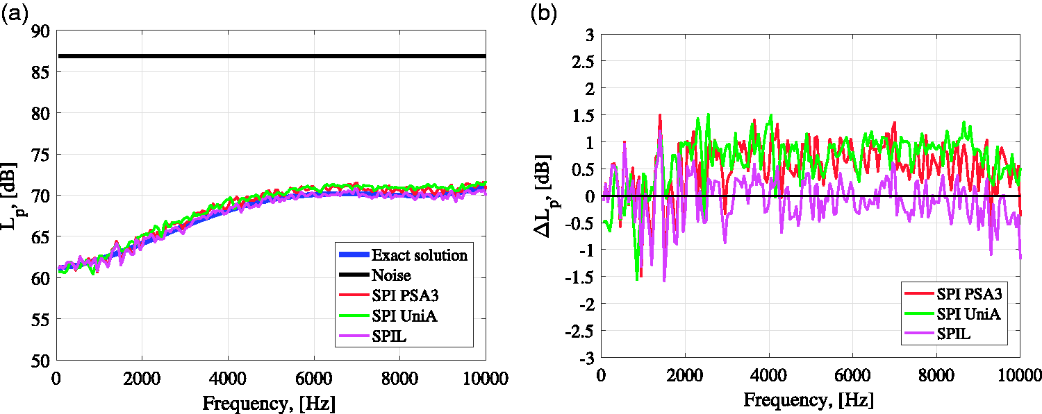
(a) Results of the line-source benchmark for the SPI and SPIL methods with w = 0.08 m. (b) Relative errors
The ISPI technique was not used in this benchmark case because all the incoherent monopoles had the same strength, and in this situation the ISPI technique is essentially the same as the SPIL method. A separate benchmark case to test the ISPI method is presented below.
Synthetic line-source and corner sources
Typical CFDBF acoustic images of the line source simulation with corner sources are shown in Figure 10 for different one-third-octave frequency bands. CFDBF was performed after removing the main diagonal of the CSM and correcting for the convection effects. These images show that, at low frequencies, the line source tends to be completely masked by the corner sources.
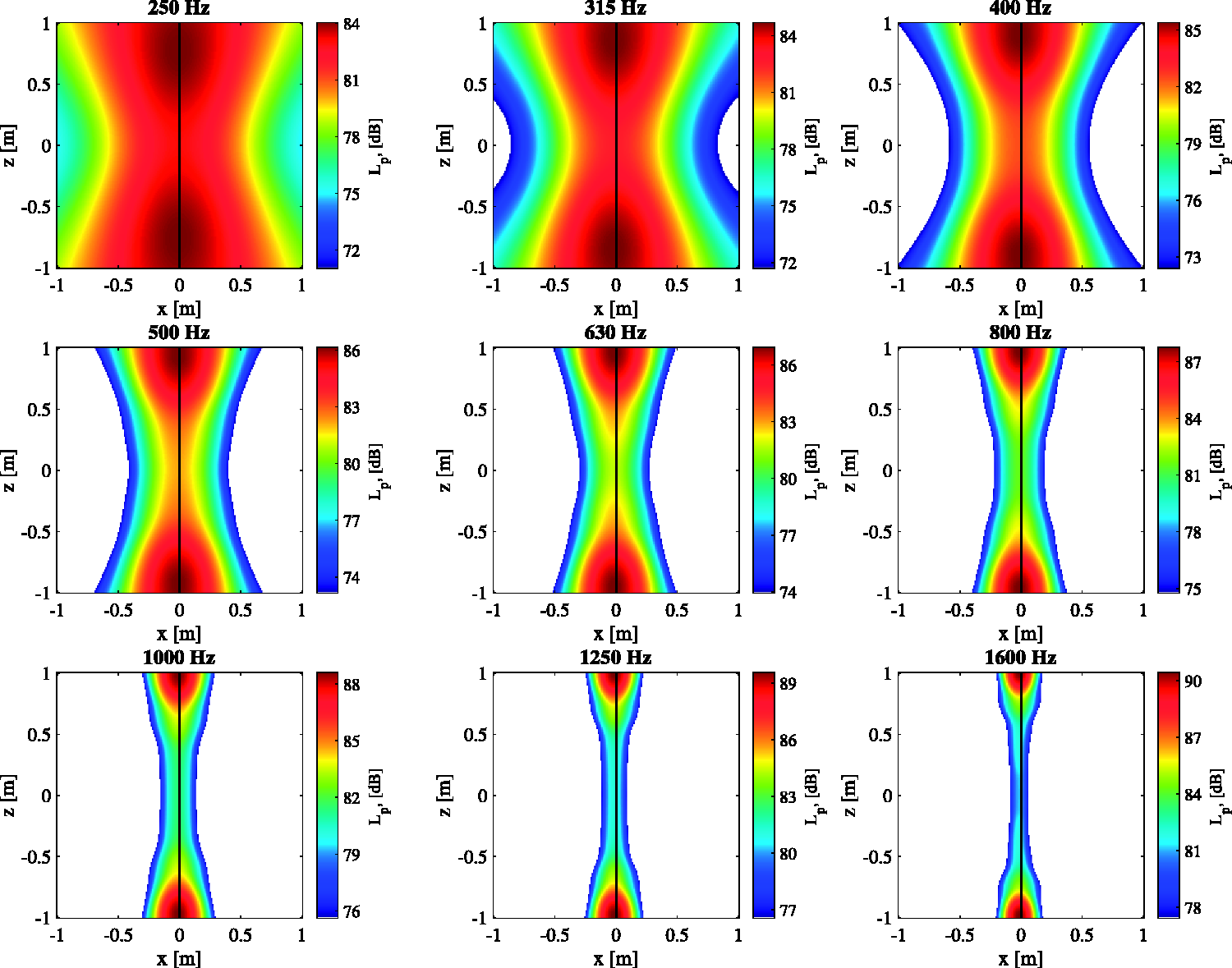
Source maps of the line source with corner sources obtained with CFDBF with DR for different one-third-octave frequency bands, with the respective center frequencies stated above each plot. The location of the line source is plotted as a solid black line.
An often-used workaround for dealing with corner sources is to perform SPI on a reduced integration area in the middle of the span, away from the corners.
51
Due to the fact that 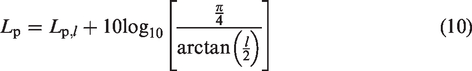
To demonstrate the added value of the ISPI method, 5 ROIs were defined (see Figure 11(a)). The span was divided into three segments. Furthermore, two ROIs were defined around the corner source locations. The width of the ROIs for all cases was w = 0.04 m and the mesh size was A central ROI that goes from Two lateral ROIs that go from Two corner ROIs at z = – 1 m and z = 1 m, respectively.
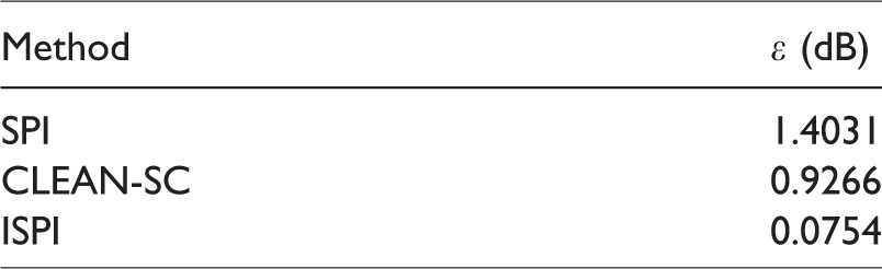
Figure 11 shows the ISPI and the SPI results of the mid-span integration area. Results obtained with CLEAN-SC are included as well. All results were corrected for full span conditions, using equation (10). It is observed that both SPI and CLEAN-SC fail at low frequencies, say below 700 Hz. The ISPI results, however, show very small errors (with maximum differences per frequency of 0.18 dB) for the full frequency range.
(a) Different ROIs considered for the ISPI method; (b) results of the line-source with corner sources benchmark for the SPI, CLEAN-SC, and ISPI methods with w = 0.04 m.
The average absolute errors ε made by each method are gathered in Table 3. The three methods show relatively small errors, although for frequencies lower than 700 Hz, SPI considerably overpredicts the results and CLEAN-SC shows an oscillating behavior. The results obtained with the ISPI technique collapse almost perfectly with the exact solution.
Average absolute errors made by each method with respect to the exact solution.
Sensitivity analysis for SPIL
A sensitivity analysis was performed for the SPIL method to investigate the influence of the parameters defining the ROI. Only the SPIL method is studied here for brevity reasons, but sensitivity analyses for the SPI and ISPI techniques are expected to provide similar results. The ROI in Figure 3 (shaded in orange) has four main parameters:
The width in the chordwise direction w. The length in the spanwise direction l. The spacing between grid points The location of the simulated line source chosen by the user x0.
For simplicity sake, only integration lines parallel to the “real” line source are considered. This assumption is easily fulfilled in practical experiments where, even though the exact locations of the noise sources are not known a priori, the orientation of the model (such as an airfoil) with respect to the microphone array can be accurately determined. Moreover, all the ROIs considered here are symmetric with respect to the z = 0 plane and are contained in the y = 0 plane, i.e. the correct source distance to the array. The influence of the distance of the scan plane to the array was not investigated in this paper, but it has been previously addressed in the literature.
62
Chordwise extension
Different ROI widths w were tested (considering
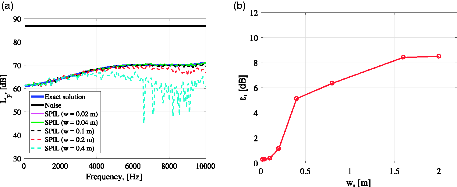
(a) Results of the sensitivity analysis performed for the SPIL method with respect to the ROI width w. Adapted from Sarradj et al.
25
(b) Average absolute errors ε made for each width case. For these results
Spanwise extension
As it was explained in equation (10),
To investigate the influence of the choice of the ROI length, several tests were performed using different values of l (considering
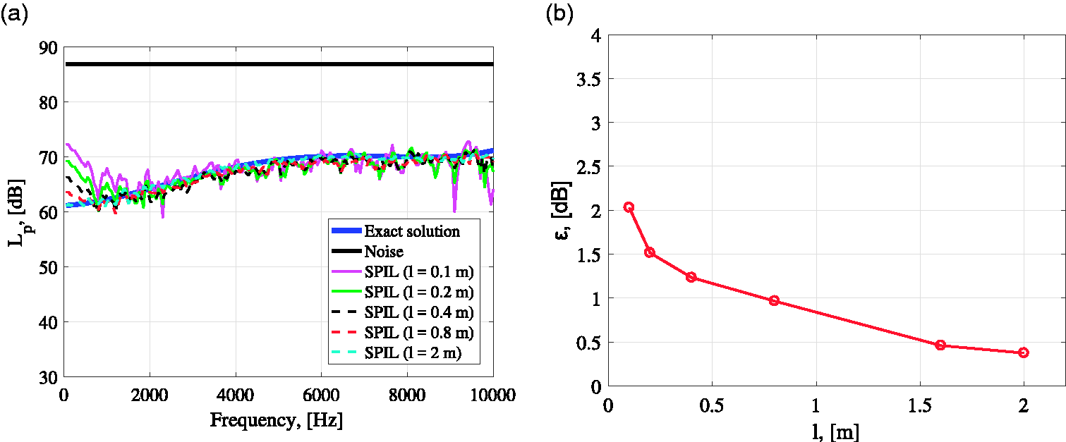
(a) Results of the sensitivity analysis performed for the SPIL method with respect to the ROI length l, corrected using equation (10). (b) Average absolute errors ε made for each length case. For these results
Mesh fineness
Tests were performed using several spacings between grid points
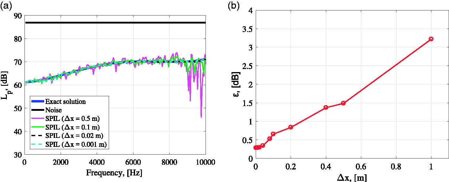
(a) Results of the sensitivity analysis performed for the SPIL method with respect to the spacing between grid points
Line source location
One of the unknowns when measuring the trailing-edge noise in aeroacoustic experiments is the exact location of the line source. To analyze the robustness of the SPIL method with respect to this variable, several tests were performed considering different locations of the simulated line source x0 (see Figure 3). The length of the ROI and mesh fineness were kept constant as l = 2 m and
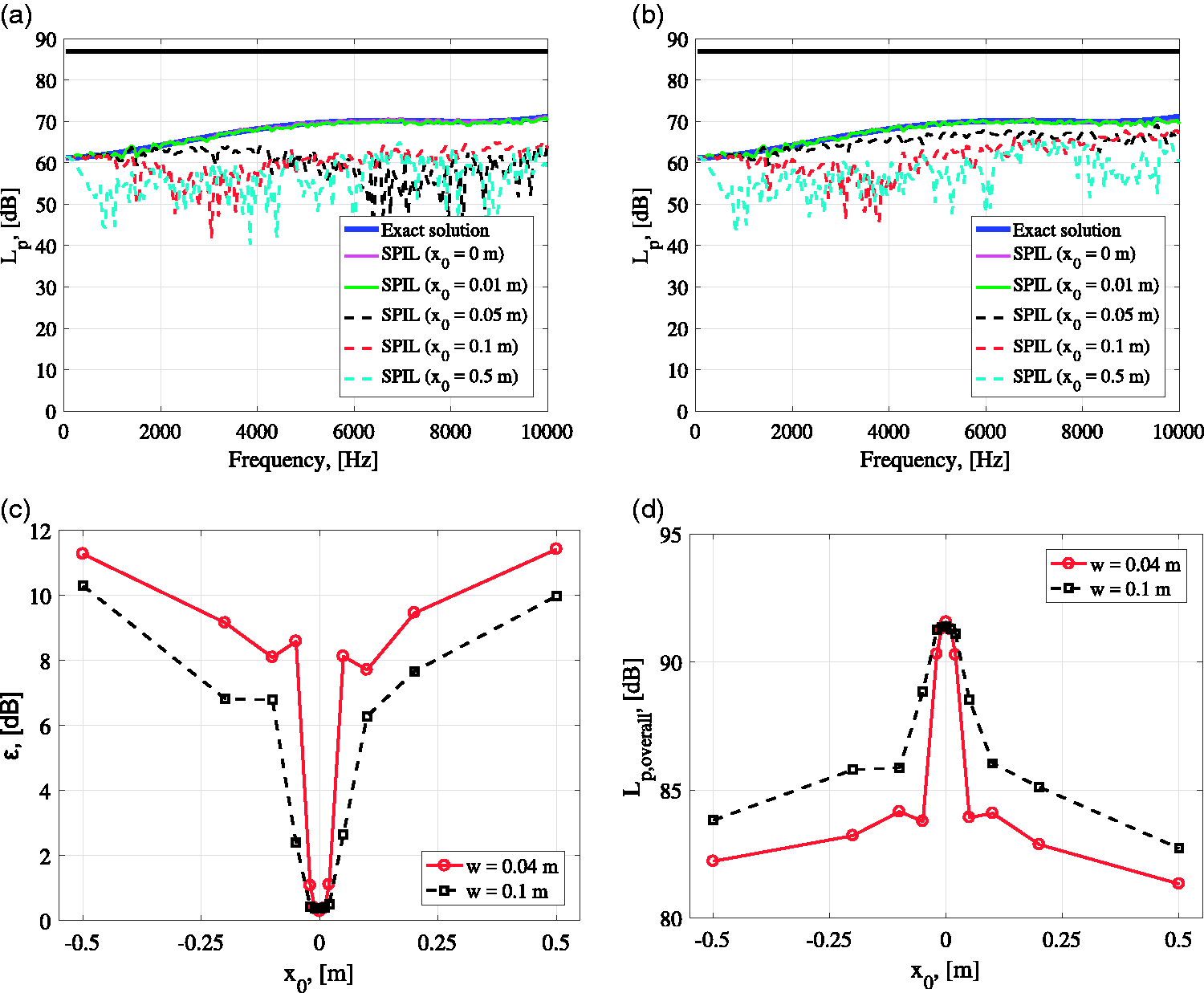
Results of the sensitivity analysis performed for the SPIL method with respect to the error in the line location x0 for (a) w = 0.04 m and (b) w = 0.1 m. (c) Average absolute errors ε and (d)
Figure 15(c) depicts the values of ε for different values of x0 for both cases of w. An almost-symmetric behavior with respect to
Figure 15(d) presents the
Since this parameter seems to be the most sensitive for the performance of the SPIL method, it is further investigated in the Experimental results section with an actual trailing-edge noise experiment. The application of porous material inserts is expected to change the location of the line source causing trailing-edge noise. 42
A similar analysis was performed with the ISPI method with the same simulated setup as before by defining several ROIs parallel to and of the same size as those defined in Figure 11(a) in the streamwise direction in order to estimate the location of the “real” line source. In this study, only the ROI covering the actual source positions provided the correct sound levels, whereas the rest of the ROIs only gave sound level values close to zero. This shows again the added value of the ISPI method with respect to other integration techniques.
Experimental results
Figure 16 depicts two CFDBF source plots for the trailing-edge noise measurements in the wind tunnel: one for the solid trailing edge (Figure 16(a)) and one for the porous trailing edge (Figure 16(b)). Both plots correspond to a flow velocity of
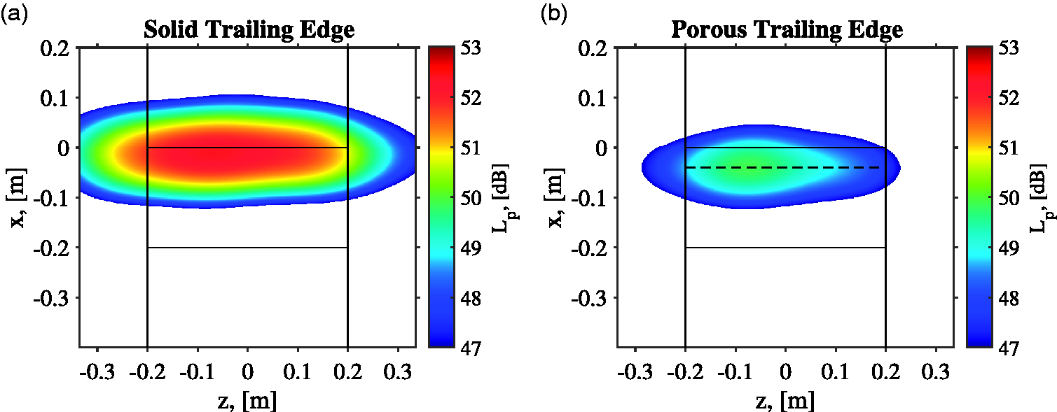
CFDBF source plots for a onetsesedtys.292 band with center frequency of 1600 Hz for
Following the guidelines proposed in the Sensitivity analysis for SPIL section, Figure 17(a) shows the
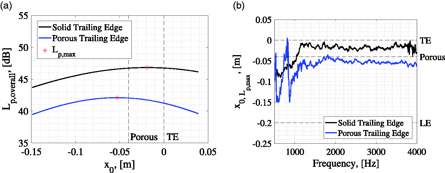
(a)
In order to study this phenomenon in detail, the x0 values for which the maximum
With the calculated values of x0 presented in Figure 17(b), the trailing-edge noise emissions can be estimated using equation (4) and scaled to decibels using equation (7). Figure 18 depicts the estimated noise emissions for both trailing-edge cases using the chord-based Strouhal number,
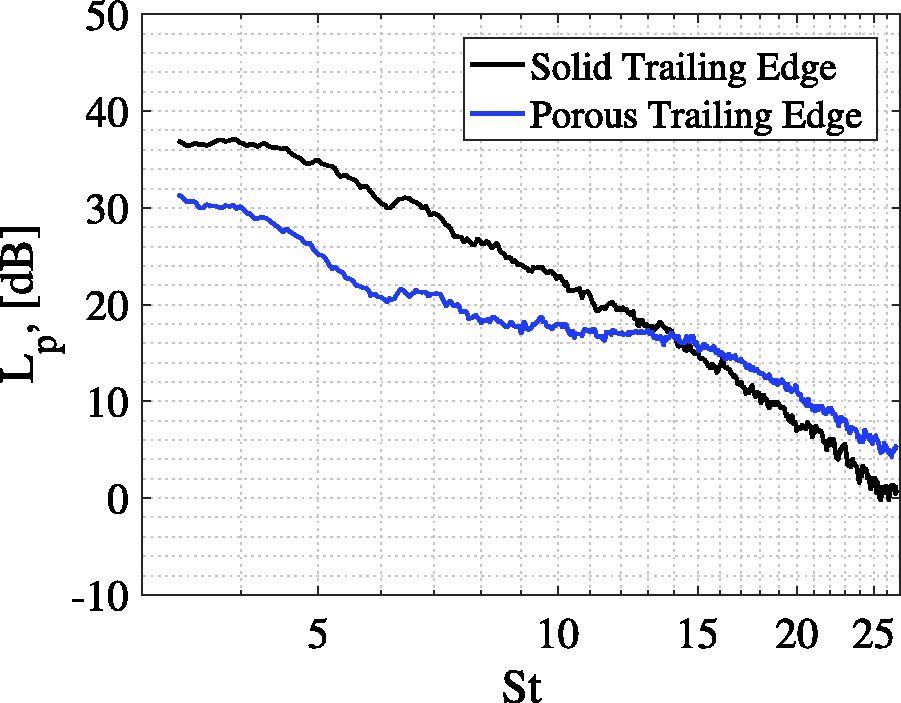
Integrated (using the SPIL technique) narrow-band spectra of the trailing-edge noise for both cases at
Figure 19 shows the relative noise reductions
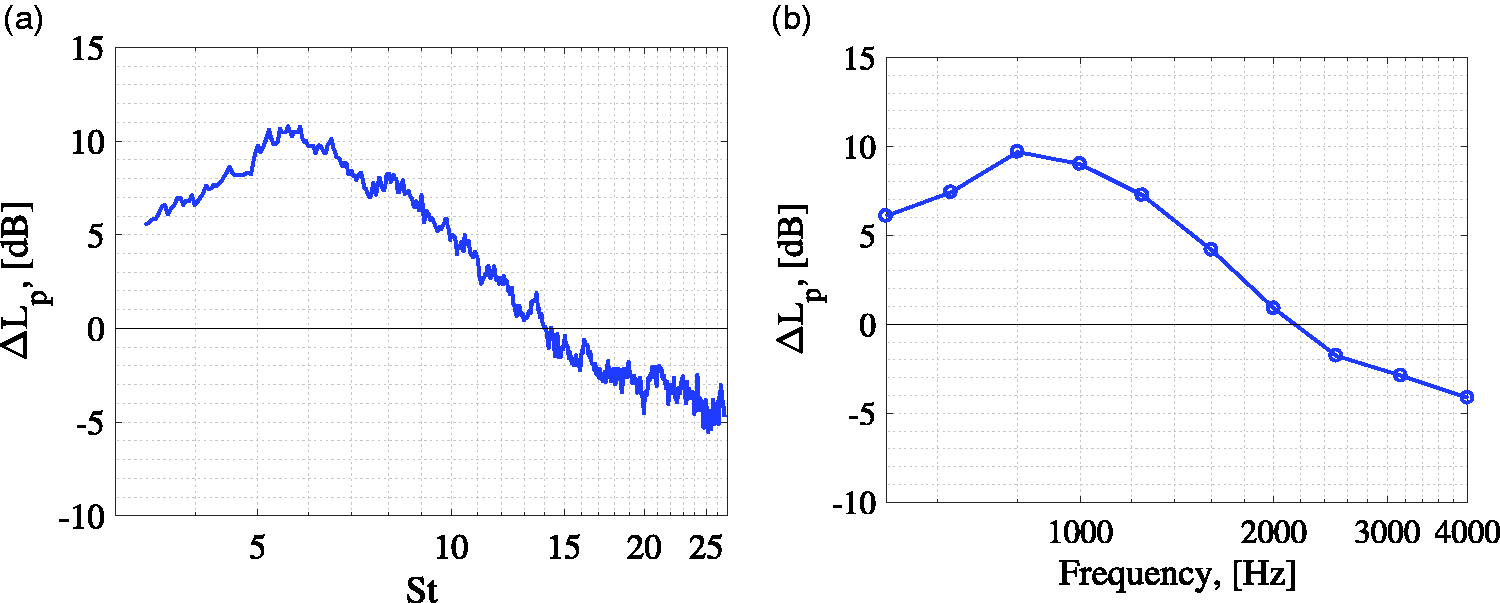
Relative noise reductions achieved by the porous trailing edge at
Conclusions
In this paper, three integration methods intended to accurately solve distributed sound sources, such as trailing-edge noise are introduced. The first technique (SPI) is based on a single monopole source, the second one (SPIL) considers the presence of a single line source, whereas the last one (ISPI) extends the assumption to several line sources.
Explanations about how the methods work are provided and the performance of each method is evaluated in two simulated benchmark cases and compared to other well-known acoustic imaging techniques. Both benchmark cases represent examples of practical wind-tunnel measurements of trailing-edge noise. SPIL showed the best performance for the first benchmark case with respect to other methods, such as DAMAS, CLEAN-SC, or functional beamforming. ISPI outperformed SPI and CLEAN-SC, allowing for the exclusion of unwanted noise sources, such as corner sources, which are usually present in the junction between the airfoil and the wind-tunnel walls. The computational demand for the three techniques is considerably low since they are based on the CFDBF algorithm.
A sensitivity analysis for the SPIL method showed that it is considerably robust to the choice of the integration area, in both shape and position. The fineness of the grid does not seem to influence the results within a sensible range. The considered position for the simulated line source was determined to be the most sensitive parameter. Recommendations are provided for practical cases.
The SPIL method was applied to experimental measurements of the trailing-edge noise of a NACA 0018 airfoil featuring solid and porous trailing edges. The performance of porous inserts as a noise reduction measure for low-frequency noise was confirmed and a crossover frequency was observed, after which, the noise emissions increase due to the roughness of the porous material. The location of the line source seems to be displaced in the upwind direction because of the presence of the porous insert.
All in all, the use of the SPIL technique is recommended for the study of distributed sound sources with little variation in the sound level and, in case the presence of unwanted noise sources, such as corner sources, is expected, ISPI is the preferred method.
Footnotes
Declaration of conflicting interests
The author(s) declared no potential conflicts of interest with respect to the research, authorship, and/or publication of this article.
Funding
The author(s) received no financial support for the research, authorship, and/or publication of this article.