Interactively visualizing distributional regression models with distreg.vis

Abstract

A newly emerging field in statistics is distributional regression, where not only the mean but each parameter of a parametric response distribution can be modelled using a set of predictors. As an extension of generalized additive models, distributional regression utilizes the known link functions (log, logit, etc.), model terms (fixed, random, spatial, smooth, etc.) and available types of distributions but allows us to go well beyond the exponential family and to model potentially all distributional parameters. Due to this increase in model flexibility, the interpretation of covariate effects on the shape of the conditional response distribution, its moments and other features derived from this distribution is more challenging than with traditional mean-based methods. In particular, such quantities of interest often do not directly equate the modelled parameters but are rather a (potentially complex) combination of them. To ease the post-estimation model analysis, we propose a framework and subsequently feature an implementation in R for the visualization of Bayesian and frequentist distributional regression models fitted using the bamlss, gamlss and betareg R packages.

1 Introduction

For modelling parameters beyond the mean of a target distribution, generalized additive models for location, scale and shape (GAMLSS) as introduced by (Rigby and Stasinopoulos, 2005) provide the ability to link all parameters characterizing the response distribution to a set of explanatory variables via an additive predictor, similar in spirit to generalized additive models but without its distributional limitations. Overcoming some of GAMLSS’ earlier restrictions, distributional regression as coined by (Klein et al., 2015c) presents a highly flexible modelling framework with a variety of possible target distributions and a wide range of effects including parametric penalized splines, random and spatial effects as well as nonparametric effects such as regression trees.

Implementations of distributional regression models feature gamlss (Stasinopoulos and Rigby, 2007) and bamlss (Umlauf et al., 2018), the most prominent extensions with a vast selection of available distributions and effects. A number of software extensions have also been developed to support specific instances of the distributional regression class, such as betareg (Grün et al., 2012) for beta regression. While gamlss and betareg employ different types of maximum likelihood estimation, bamlss implements a Bayesian approach featuring posterior mode estimates which are subsequently used as starting values for Markov chain Monte Carlo (MCMC) sampling. This has the added benefit of being able to construct the posterior distribution of each parameter as well as potentially complex functions of these parameters.

Moving beyond single-parameter regression models naturally leads to additional challenges when it comes to the interpretation of the estimated effects since the same covariate may show up in multiple regression predictors and applying a non-identity link function additionally makes the interpretation depend on the remaining set of covariates. Furthermore, in many cases the parameters employed to characterize the distribution of interest do not directly equate the moments or other interpretable characteristics of a distribution, making another transformation necessary to arrive at interpretable figures.

As a consequence, applied researchers often appreciate the practical appeal of distributional regression where regression relations beyond the mean can be investigated but they struggle when it comes to understanding the output of the regression estimates. To facilitate this process, we introduce a new package distreg.vis that can deal with model classes from the bamlss, gamlss and betareg packages to achieve the following tasks:

moments: Obtain predicted moments (Expected Value, Variance) of the target distribution based on user-specified values of the explanatory variables, if they exist.

plot_dist: Create a graph displaying the predicted probability density function or cumulative distribution function based on the same user-specified values.

plot_moments: View the marginal influence of a selected effect on the predicted moments of the target distribution.

With those functions, applied scientists can directly translate regression objects into publication-ready graphs without the need to worry about package-specific predict and plotting functions, the connection between predicted parameters and moments or the correct display of predicted probability density functions. To make the process of interpreting fitted distributional regression models even more accessible, distreg.vis features a rich Graphical User Interface (GUI) built on the shiny framework (Chang et al., 2018). Using this GUI, the user can (a) obtain an overview of the selected model fit and then use the functions mentioned above to (b) easily select explanatory values for which to display the predicted distributions, (c) obtain marginal influences of selected covariates and (d) change aesthetical components of each displayed graph. After a successful analysis, the user can obtain the R code needed to reproduce all displayed plots, without having to start the application again.

The idea of calculating conditional values of the response distribution by way of plot_moments() is not new. In fact, many other R packages feature aspects of the functionality of distreg.vis. Notably, the effects package (Fox and Weisberg, 2019)) is an extensive library for calculating conditional means of the response distribution depending on varying explanatory covariates in linear, generalized linear and mixed effects-type models. Lacking the graphing capabilites of effects while putting more focus on the estimation of marginal means, the prediction (Leeper, 2019) package offers a bigger range of supported model classes and even non-parametric effects.

Certainly the most general marginal effects packages are emmeans (Lenth, 2019), formerly called lmmeans (Lenth, 2016), and ggeffects (Lüdecke, 2018), as they not only offer a large variety of supported model classes and predictor effects, but contrary to effects and prediction also include the compatibility to all of distreg.vis’ supported distributional regression model classes: gamlss, betareg and bamlss (only supported by ggeffects). However, even the latter two effects packages are only able to compute marginal means of moment values for betareg and fail to provide the same functionality for bamlss and gamlss, where predictions remain restricted to the parameter-level. As such, distreg.vis is the only package which supports both gamlss, bamlss and betareg in full generality and can calculate marginal effects on the moments and not only the parameters of a distribution.

The package distreg.vis is available on the Comprehensive R Archive Network (CRAN) at https://cran.r-project.org/web/packages/distreg.vis/index.html .

The remainder of this article is structured as follows: Section 2 provides an example tutorial on analysing income distributions in which using distreg.vis yields a benefit. Section 3 covers the methodological background of the distributional regression model class and its implementations, while Section 4 offers a glimpse into the GUI. Section 5 concludes the article. The appendices provide an in-depth guide to the implementation of the two main functions of the package (Section A) and the Graphical User Interface (Section B), display special cases of distreg.vis’ functions (Section C) and provide complementary graphs (Section D). The R script including the dataset as well as the appendices are available in the online supplemental materials at http://www.statmod.org/smij/archive.html .

2 Motivating example: Drivers of yearly income

To illustrate the usefulness of distreg.vis, we will give a short example based on a dataset about the yearly income of 3,000 male workers in the Mid-Atlantic region of the United States, provided by the ISLR package (James et al., 2017). This dataset will then be used continuously throughout Sections 2 and 4 as well as parts of the Appendix to illustrate distreg.vis’ abilities.

The dataset consists of 11 variables, both continuous and categorical. Our variable of main interest, that is, the response in the following regression analyses, is given by individual's raw yearly income in thousand US$ (variable wage). The remaining variables mostly contain socioeconomic information, including the person's age in years (age), their ethnic origin (ethnicity), their level of education (education) and the year in which the observation was recorded (year). Considering its non-negative nature, we start by assuming a log-normal distribution for the wages, $y\sim \mathit{Lognormal}(\mu ,{\sigma }^2)$ . Though more complex distributions would provide a slightly better fit than the log-normal, it was chosen for its simplicity and popularity.

To find out what drives a person's income, we will link both parameters of the log-normal distribution to the aforementioned explanatory variables. The model specification therefore has the following form:

$$\begin{array}{cc}\begin{array}{cc}\hfill \mu & ={\beta }_{10}+f_{11}(\mathtt{age})+{\beta }_{12}·\mathtt{year}+f_{13}(\mathtt{education})+f_{14}(\mathtt{ethnicity})\hfill \\ \hfill \text{log}(\sigma )& ={\beta }_{20}+f_{21}(\mathtt{age})+{\beta }_{22}·\mathtt{year}+f_{23}(\mathtt{education})+f_{24}(\mathtt{ethnicity})\hfill \end{array}\hfill & \hfill \end{array}$$

(2.1)

where the functions $f_{11},f_{21}$ are modelled nonparametrically using penalized splines (Eilers and Marx, 1996), while $f_{13},f_{23},f_{14}$ and $f_{24}$ are modelled as simple fixed categorical effects of the respective variables. All effects with more than one degree of freedom are therefore consistently denoted with $f_{\mathit{ij}}(·)$ to emphasize that the original input variable has to be recoded prior to inclusion in the model. The standard deviation parameter $\sigma$ is connected to the explanatory variables using a log-link function to ensure a positive support.

Combined with the sample-based estimation technique of bamlss, distreg.vis can produce credible intervals around marginal influence plots. For this reason, we choose bamlss for model estimation, using the following code:

R> wage_model – bamlss(

+ list(

+ wage ~ s(age) + ethnicity + year + education,

+ sigma ~ s(age) + ethnicity + year + education

+),

+ data = Wage,

+ family = lognormal_bamlss

+)

After successful estimation, it makes sense to have a look at the model summary. Using the built-in summary.bamlss function, we can take a look at the results:

R> print(summary(wage_model), digits = 1)

[output shortened]

Formula mu:

—

wage ~ s(age) + ethnicity + year + education

-

Parametric coefficients:

Mean 2.5 (Intercept) 36.834 14.075 36.606 61.579 38.0

ethnicity2. Black 0.008 -0.077 0.007 0.101 0.0

[output shortened]

-

Smooth terms:

Mean 2.5 s(age).tau21 0.33 0.06 0.23 1.21 0.3

s(age).alpha 1.00 1.00 1.00 1.00 NA

s(age).edf 5.99 4.52 5.96 7.63 6.4

—

Formula sigma:

—

sigma ~ s(age) + ethnicity + year + education

-

Parametric coefficients:

[output shortened]

-

Smooth terms:

Mean 2.5 s(age).tau21 2.5 0.5 2.0 7.7 2

s(age).alpha 0.9 0.4 1.0 1.0 NA

s(age).edf 6.3 4.7 6.3 7.6 6

—

[output shortened]

As visible in the code output, bamlss provides estimation results for each effect used to describe the target distribution parameters ( $\mu$ and $\sigma$ in this case). Even though making statements about each effects’ significant difference from zero is possible, the interpretation of such statements as well as for the raw effect estimates is difficult. Model results of penalized splines, for example, only show estimates for their degree of smoothness ( $\tau$ and $\alpha$ ) and estimated degrees of freedom. Without appropriate graphs showing the marginal effect they can therefore not be interpreted. Furthermore, even the absolute coefficients for the categorical effects cannot be taken at face value, since they only affect the distributional parameters $\mu$ and $\sigma$ , and not the moments.

To overcome these limitations, we use distreg.vis. If, for example, we are interested in the impact of education on the marginal income distribution, we create a data.frame object in which all different education categories are present and all other numeric variables are set to their mean. This can be easily achieved by the function set_mean() in combination with model_data, which obtains the explanatory covariates of the model and sets them to the mean. Further defining the row.names of the data.frame to be the different education levels ensures improved legends in further graphs.

R> df <– set_mean(

+ model_data(wage_model),

+ vary_by = “education”

+)

R> row.names(df) <– levels(Wage$education)

R> df

ethnicity year education age

1. < HS Grad 1. White 2006 1. < HS Grad 42

2. HS Grad 1. White 2006 2. HS Grad 42

3. Some College 1. White 2006 3. Some College 42

4. College Grad 1. White 2006 4. College Grad 42

5. Advanced Degree 1. White 2006 5. Advanced Degree 42

Now, it will be interesting to see the predicted distribution for all five cases. To achieve this, we first use distreg.vis‘ preds() function and obtain the predicted distributional parameters. Then, we include them into plot_dist() to plot the complete distributions:

R> pp <– preds(model = wage_model, newdata = df)

R> pp

mu sigma

1. < HS Grad 4.485241 0.2691822

2. HS Grad 4.603004 0.2886467

3. Some College 4.722890 0.2826761

4. College Grad 4.836627 0.3278559

5. Advanced Degree 5.002570 0.3490710

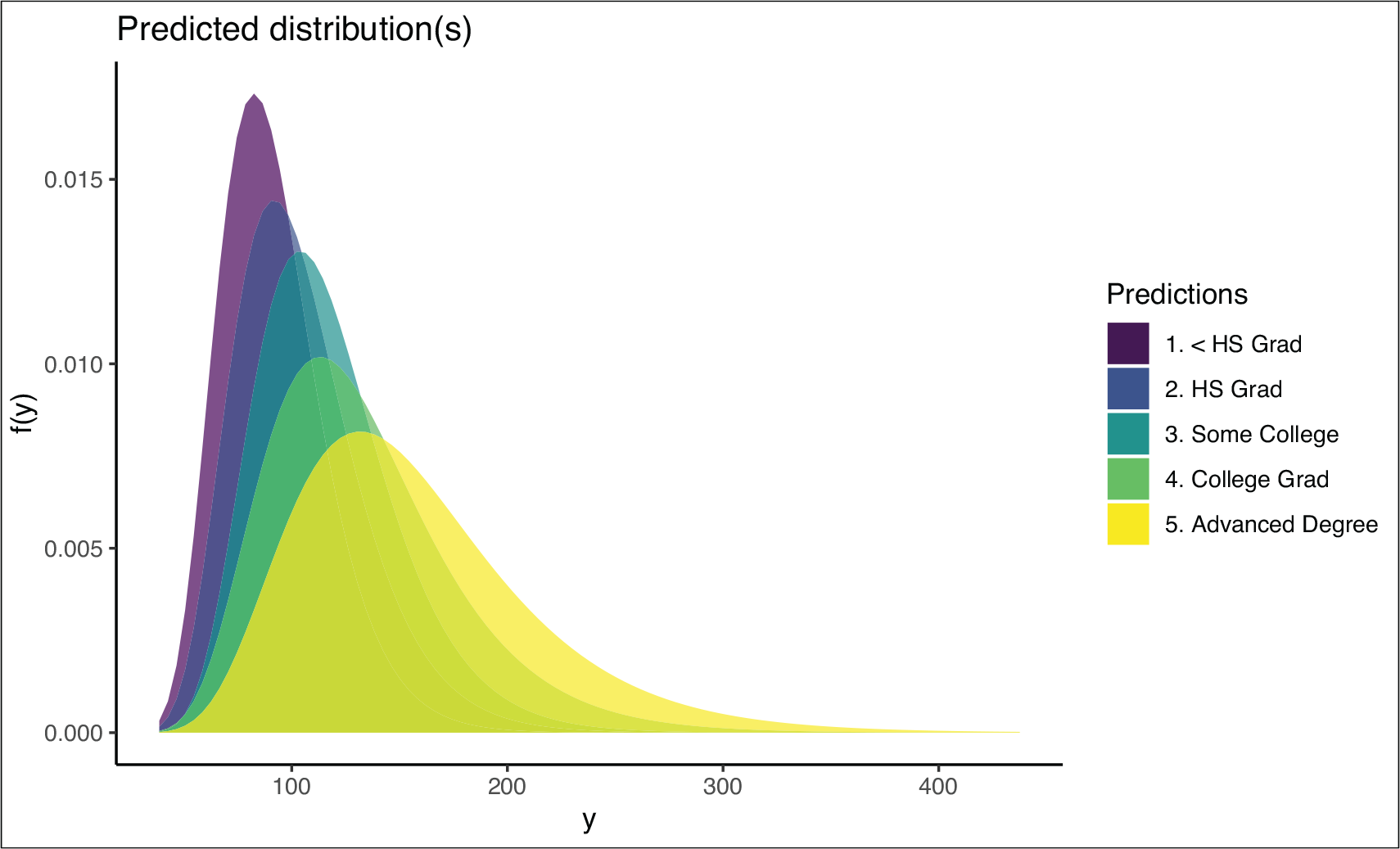
R> plot_dist(wage_model, pred_params = pp)

Figure 1

Predicted distributions for each covariate combination specified in the df data.frame object

Figure 1 displays the predicted distributions for each covariate combination specified in df. We can see that the predicted income not only changes in location (higher education shifts the distribution to the right) but also in the variance (higher education leads to a lower variance).

Figure 1 is useful to get a visual feel of the influence of education on the modelled distribution. However, we would also like to know the influence of age, which is not a categorical covariate, on the predicted moments of the log-normal distribution. Normally, this would be a tedious task, as the modelled non-parametric effect has to be transformed two times: First, via the link function to ensure the correct support of the modelled parameters. And second, from the parameters to the distributional moments, as the parameters of the log-normal distribution do not directly equate its moments.

The function plot_moments() was written to solve this task. It takes both a fitted distributional regression object and combinations of explanatory variables for which the influence is of interest. In our case, we specify both the df and wage_model objects as arguments of the function:

R> plot_moments(

+ wage_model,

+ int_var = “age”,

+ pred_data = df,

+ rug = TRUE,

+ samples = TRUE,

+ palette = “viridis”,

+ uncertainty = TRUE

+)

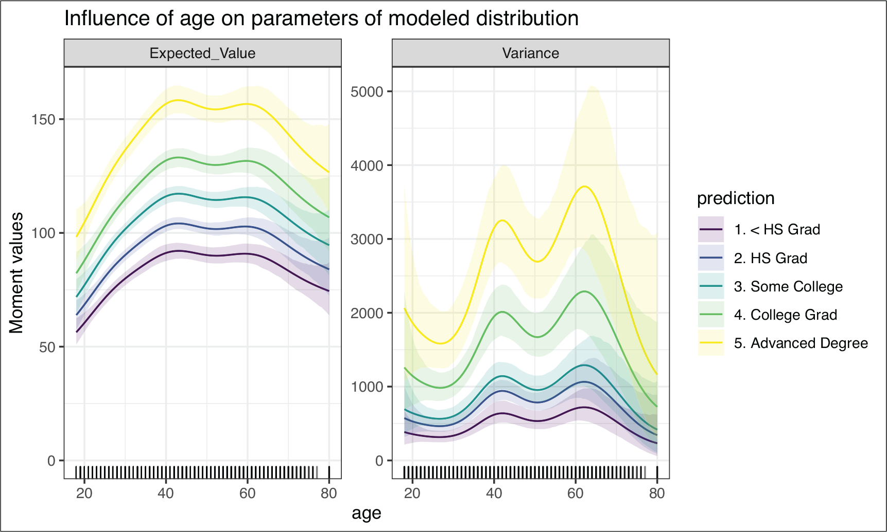
Executing the above code results in what can be seen in Figure 2. The plot is divided into two parts representing the first two moments of the target distribution labelled ‘Expected_Value’ and ‘Variance’. On both graphs, the y-axis depicts the moment values, while x-axis displays the variable of interest, which is age in our case.

Figure 2

Impact of variable age on the first two predicted moments of the target wage distribution, including its 95% credible intervals

The lines seen in each graph represent the previously specified covariate combinations, and then display how the moment changes over the whole range of the variable of interest. In our case the five different lines represent different education levels. We can now see that the expected wage level first rises with age until around the age of 40, when it is lowered a bit. Then the income levels increase again up until the age of 60, at which point the wage then decreases. We can also see that this shape roughly stays the same for each education level, which stems from the lack of a modelled interaction effect between age and education.

A strong advantage of the sample-based approach of bamlss is its ability to easily construct credible intervals around the parameter estimates. In Figure 2 we can see small shadows representing credible intervals above and below each of the five lines describing the age effect on the first two moments in each education category. Since the first and highest education categories do not overlap, we can conclude that their effect is significantly different from each other, just from observing the graph.

Looking at the right part of Figure 2, we can see that the modelled variance levels of the target distribution show similar linkage to age as the expected value: Two high points can be observed around the age of 40 and 60, both at which the modelled distribution reaches the highest wage variance.

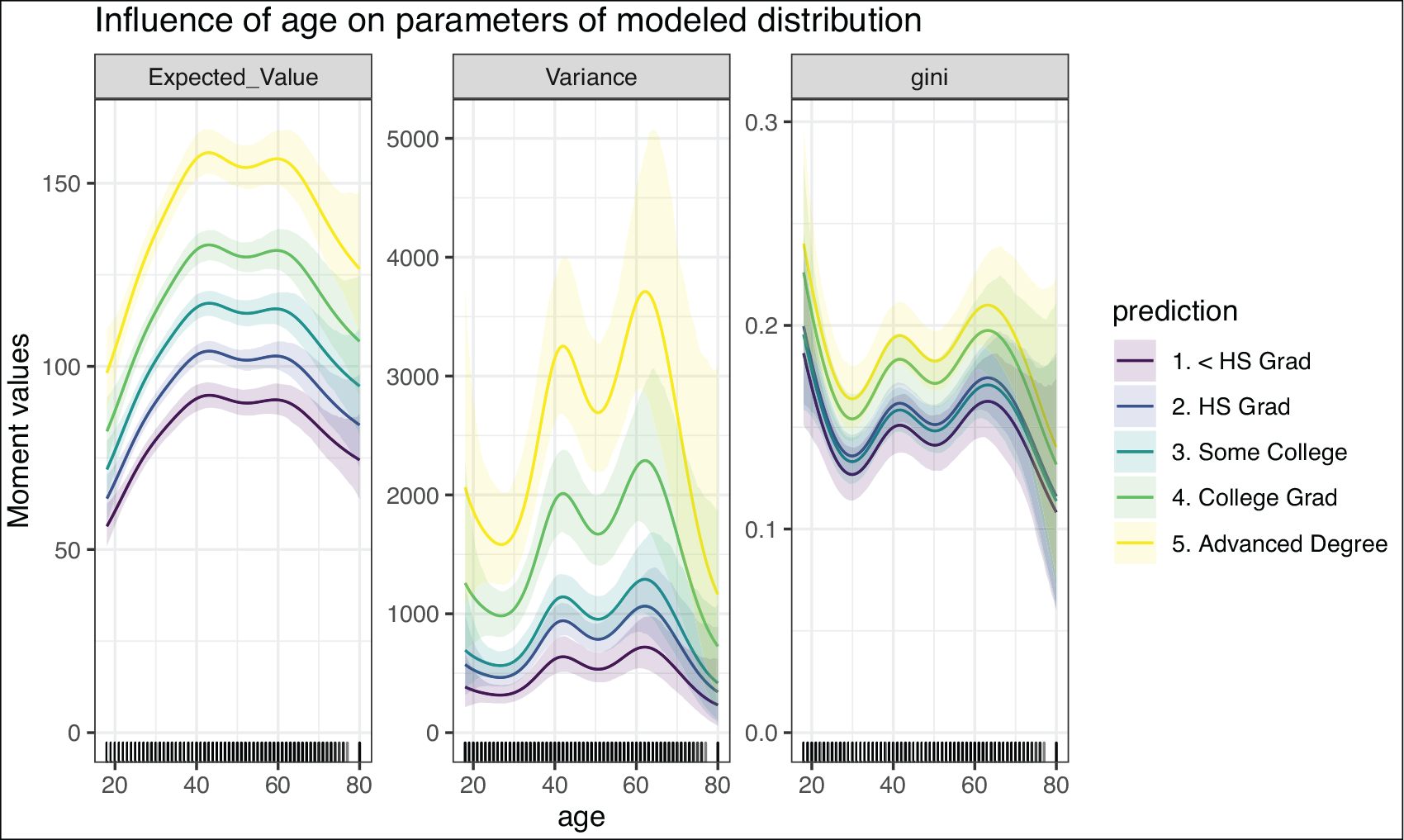
Even though Figure 2 only shows the influence of age on the first two moments, plot_moments() is easily able to include other metrics that depend on the predicted parameters, using its argument ex_fun. A good example in wage distributions would be the Gini coefficient (Lerman and Yitzhaki, 1984), an economic figure measuring a distributions’ inequality. Including this measure in our effect plots can be done using the following code:

R> gini <– function(par) {

+ 2 * pnorm((par[[”sigma”]] / 2) * sqrt(2)) – 1

+ }

R> moments_plot_exfun <– plot_moments(

+ wage_model, int_var = “age”,

+ pred_data = df, samples = TRUE,

+ uncertainty = TRUE, ex_fun = “gini”,

+ rug = TRUE

+)

Figure 3

Impact of variable age on the first two predicted moments of the target wage distribution (equivalent to Figure 2) as well as a user-specified function (gini), including its credible intervals

As visible in Figure 3, a new graph window was added in comparison to 2 depicting the influence of age on our specified metric, the Gini coefficient. Further noticable are the credible intervals which we can also obtain if we combine plot_moments() with the sample-based approach of bamlss.

The function plot_moments() is also able to display the difference in moments depending on a categorical covariate. No other arguments have to be specified – distreg.vis is able to detect the variable type automatically. In the following code chunk, the variable ethnicity is selected as the variable of interest.

R> plot_moments(

+ wage_model, int_var = “ethnicity”,

+ pred_data = df, samples = TRUE,

+ palette = “viridis”, uncertainty = TRUE

+)

Figure 4

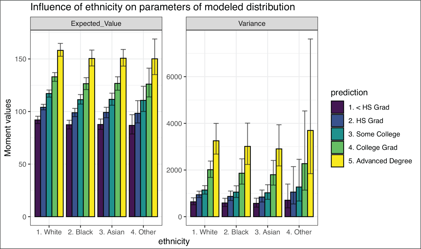
Impact of variable ethnicity on the first two predicted moments of the target wage distribution

Figure 4 now shows the result of the code chunk above. On the x-axis we can see the categories of our variable of interest, ethnicity. The y-axis now denotes the moments broken up by both the variable of interest and the categories of education, which we specified in the code chunk on page 532. The error bars on the ends of each bar represent credible intervals (95%). From analysing the bars with its error fields we can conclude that the variable education mostly yields significantly different expected values of wage, while ethnicity does not.

From the provided example on modelling wages, it became apparent that distributional regression is a useful tool to handle complex model scenarios. Nonetheless, visualizing the fitted regression models using existing tools is difficult, as transformations are necessary to arrive at interpretable figures. This process is made easier by distreg.vis, which gives the abilities to quickly visualize predicted distributions and display marginal moment influences.

3 The distributional regression model class

Distributional regression models represent an umbrella class for models where it is possible to link the parameters beyond the mean of a target distribution to available predictors (Klein et al., 2015c). Any choice of the underlying parametric target distribution is valid, as long as the probability density function is twice continuously differentiable with respect to the parameters and, in particular, is not limited to the exponential family typically employed in generalized additive models. Assuming a parametric distribution $y\sim D({\theta }_1,\dots ,{\theta }_l,\dots ,{\theta }_L)$ with $L$ distributional parameters ${\theta }_1,\dots ,{\theta }_L$ , we arrive at the model specification

$$g_l({\mathbf{\theta }}_l)=f_{1l}({\text{X}}_{1l};{\mathbf{\beta }}_{1l})+\dots +f_{Q_{l}l}({\text{X}}_{Q_{l}l};{\mathbf{\beta }}_{Q_{l}l}),$$

(3.1)

where $g_l(·)$ , $l=1,\dots ,L$ denotes the link function used to uphold the support of parameter ${\theta }_l$ , $f_{\mathit{ql}}(·)$ , $q=1,\dots ,Q_l$ represents the possibly non-parametric effect of covariate(s) ${\text{X}}_{\mathit{ql}}$ on the modelled parameter and ${\mathbf{\beta }}_{\mathit{ql}}$ , $q=1,\dots ,Q_l$ depict the regression parameters which are to be estimated.

Depending on the software package used to fit a distributional regression model, a vast selection of possible effects are available, including but not limited to penalized splines (also in multivariate forms), spatial effects based on Gaussian random fields or Markov random fields, varying coefficient terms and random effects (see Fahrmeir et al., 2013, Ch. 9 for an overview). More recently, new research is done on connecting the distributional regression framework to effects known from Machine Learning, for example, Random Forest (Schlosser et al., 2019). Multivariate extensions have also gained considerable interest in the past, see for example Klein et al., 2015a, Klein and Kneib, 2016) or (Marra and Radice, 2017).

Due to the high flexibility in the target distributions, the predictors and the specified link function, distributional regression encompasses many well-known regression approaches, such as generalized linear models (Nelder and Wedderburn, 1972, GLM), generalized additive models (Hastie and Tibshirani, 1990, GAM), generalized additive mixed models (Lin and Zhang, 1999 GAMM) and generalized additive models for location, scale and shape (Rigby and Stasinopoulos, 2005, GAMLSS). Although in theoretical proximity to GAMLSS, the term distributional regression was coined since distributional parameters do not always represent either the location, scale or shape of a distribution (Klein et al., 2015c).

3.1 Implementations of GAMLSS

For estimating distributional regression models in R, the two most capable software implementations are gamlss (Stasinopoulos and Rigby, 2007) and bamlss (Umlauf et al., 2018), with the package betareg (Grün et al., 2012) only focusing on beta regression. The main difference in gamlss and bamlss are rooted in their estimation techniques, which will be described below:

gamlss

The gamlss package features a frequentist approach employing (penalized) maximum likelihood inference. Its main estimation algorithm RS, short for Rigby and Stasinopoulos, uses iteratively reweighted least squares (IRLS) in combination with a modified backfitting algorithm to arrive at coefficient estimates. The algorithm system is broken up into inner and outer iterations, with each inner iteration depicting the fitting of one distributional parameter ${\theta }_l$ . Here, a working variable ${\text{z}}_l$ consisting of all used predictors, the first derivative of the likelihood (score function) and ‘iterative weights’ ${\text{w}}_l$ , determined with a local scoring algorithm, is calculated. Then, the working variable is fitted to the explanatory variables using backfitted weighted least squares and penalized weighted least squares for parametric and non-parametric coefficients, respectively. The inner iteration is repeated until the inner global deviance has converged. This procedure is done for every ${\theta }_l$ , after which one outer iteration is finished. The outer iterations are further repeated, until the outer global deviance has also converged (Ch. 3 Stasinopoulos et al., 2017).

Estimating parameters with backfitting has the advantage of avoiding the need for cross-derivatives and is therefore quite efficient. Uncertainty assessments typically rely on asymptotic normality assumptions and have been found to be pretty conservative in simulation studies (see, for example, Klein et al., 2015b).

The collection of gamlss packages provides a vast number of distributions via its accompanying package gamlss.dist (Stasinopoulos and Rigby, 2019) as well as several extensions concerning spatial data effects (gamlss.spatial, De Bastiani et al., 2018) or truncated distributions (gamlss.tr, Stasinopoulos and Rigby, 2018), for example.

bamlss

The bamlss package (Umlauf et al., 2018) provides a highly customizable Bayesian estimation framework with both posterior mode estimates via penalized likelihood and fully Bayesian inference implemented via MCMC simulation techniques. By default, it revolves mainly around two functions: bamlss::bfit() and bamlss::GMCMC(). The first function, bfit(), utilizes an optimizing function which seeks to find the mode of the posterior distribution via penalized likelihood with respect to the effect coefficients. Then, those values are used as starting numbers for MCMC simulations (function GMCMC()), which are based on iteratively weighted least squares proposals that rely on multivariate normal proposals obtained from locally quadratic approximations of the log-full conditional (Brezger and Lang, 2006).

Both functions can be swapped by the user with optimizer and sampler functions that more closely resemble the subjective preference. As such, the implementation of bamlss represents a lego-type toolbox that enables replacing specific parts of the model specification with alternative and potentially more flexible variants without altering the rest of the model implementation. Compared to gamlss, the number of supported distributions is more limited but the access to posterior samples facilitates finite sample inference also for complex functionals of the original parameters. Default priors are assigned to all parameters of the model specification but these can also be controlled by the user.

3.2 Distributional compatibility

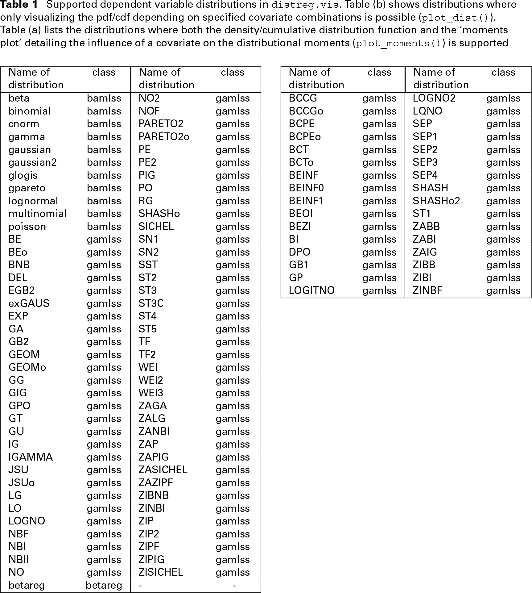
To ensure a wide user audience, distreg.vis is able to support a variety of distributions from the gamlss, bamlss and betareg packages. Table 1 gives an overview, and divides the available distributions into those that can be used in both plot_dist() and plot_moments() (Table 1a), and those that can only be used in combination with plot_dist() (Table 1b). Table 1b consists of distributions which do not have existing moments or do not have any implementations yet, rendering them incompatible with plot_moments(). To include as many distributional families as possible, we worked together with both the authors of gamlss (Stasinopoulos and Rigby, 2007) and bamlss (Umlauf et al., 2018) and implemented the moment functions for almost all available distributions in their respective packages.

Table 1

Supported dependent variable distributions in distreg.vis. Table (b) shows distributions where only visualizing the pdf/cdf depending on specified covariate combinations is possible (plot_dist)(). Table (a) lists the distributions where both the density/cumulative distribution function and the ‘moments plot’ detailing the influence of a covariate on the distributional moments (plot_moments()) is supported

Name of distribution	class	Name of distribution	class
beta	bamlss	NO2	gamlss
binomial	bamlss	NOF	gamlss
cnorm	bamlss	PARETO2	gamlss
gamma	bamlss	PARETO2o	gamlss
gaussian	bamlss	PE	gamlss
gaussian2	bamlss	PE2	gamlss
glogis	bamlss	PIG	gamlss
gpareto	bamlss	PO	gamlss
lognormal	bamlss	RG	gamlss
multinomial	bamlss	SHASHo	gamlss
poisson	bamlss	SICHEL	gamlss
BE	gamlss	SN1	gamlss
BEo	gamlss	SN2	gamlss
BNB	gamlss	SST	gamlss
DEL	gamlss	ST2	gamlss
EGB2	gamlss	ST3	gamlss
exGAUS	gamlss	ST3C	gamlss
EXP	gamlss	ST4	gamlss
GA	gamlss	ST5	gamlss
GB2	gamlss	TF	gamlss
GEOM	gamlss	TF2	gamlss
GEOMo	gamlss	WEI	gamlss
GG	gamlss	WEI2	gamlss
GIG	gamlss	WEI3	gamlss
GPO	gamlss	ZAGA	gamlss
GT	gamlss	ZALG	gamlss
GU	gamlss	ZANBI	gamlss
IG	gamlss	ZAP	gamlss
IGAMMA	gamlss	ZAPIG	gamlss
JSU	gamlss	ZASICHEL	gamlss
JSUo	gamlss	ZAZIPF	gamlss
LG	gamlss	ZIBNB	gamlss
LO	gamlss	ZINBI	gamlss
LOGNO	gamlss	ZIP	gamlss
NBF	gamlss	ZIP2	gamlss
NBI	gamlss	ZIPF	gamlss
NBII	gamlss	ZIPIG	gamlss
NO	gamlss	ZISICHEL	gamlss
betareg	betareg	-	-
BCCG	gamlss	LOGNO2	gamlss
BCCGo	gamlss	LQNO	gamlss
BCPE	gamlss	SEP	gamlss
BCPEo	gamlss	SEP1	gamlss
BCT	gamlss	SEP2	gamlss
BCTo	gamlss	SEP3	gamlss
BEINF	gamlss	SEP4	gamlss
BEINF0	gamlss	SHASH	gamlss
BEINF1	gamlss	SHASHo2	gamlss
BEOI	gamlss	ST1	gamlss
BEZI	gamlss	ZABB	gamlss
BI	gamlss	ZABI	gamlss
DPO	gamlss	ZAIG	gamlss
GB1	gamlss	ZIBB	gamlss
GP	gamlss	ZIBI	gamlss
LOGITNO	gamlss	ZINBF	gamlss

4 Introduction of the graphical user interface

To understand the fit of the predicted distribution and the magnitude of included effects, plot_dist() and plot_moments() are powerful tools. However, constructing the correct scenarios and specifying them in the appropriate data.frame format takes time. Furthermore, the resulting graphs are then static, as changing the scenarios each time after viewing the results is a slow process.

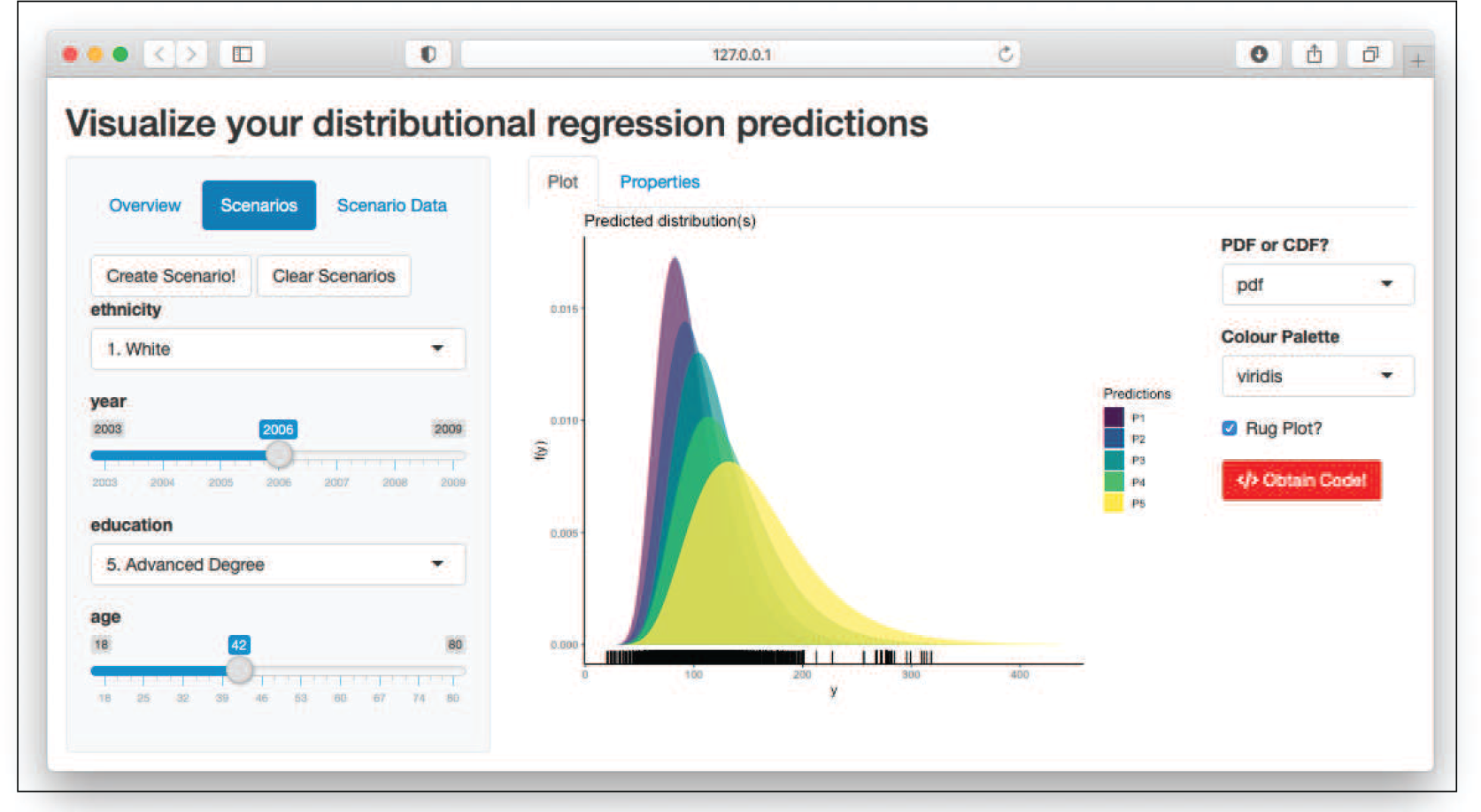
To make using distreg.vis as uncomplicated as possible, it features a rich Graphical User Interface, in which the user can select his/her covariate scenarios and produce publication-ready graphs interactively. In doing so, distreg.vis is strongly based on shiny (Chang et al., 2018), which is an R package designed to create interactive visualizations with HTML code and R functions.

Figure 5

Plot tab output when specifying five different scenarios with different education levels

In its core, a shiny application is built using R functions and can therefore be called similarly. In the case of distreg.vis, there are two ways one can start the application. First, the user can run the function vis(). Second, it can also be called using the open source Graphical User Interface RStudio (RStudio Team, 2020). When opened, one can click on the ‘Add-Ins’ button and then select ‘Distributional Regression Model Visualizer’ if distreg.vis is installed (Figure D10 in the Appendix). This will also trigger the function vis().

To give a short glimpse on the look of the GUI, Figures 5 and 6 are provided. In both figures Section 2’s analysis was repeated using the interactive GUI. Specifically, in Figure 5 the covariate combinations with only education levels varying were interactively specified, leading to the same values as on page 532. Defining all five covariate combinations leads to its predicted distributions appearing on the right side of the interface, the graph of which is then also a direct copy of Figure 2 from Section 2.

Figure 6

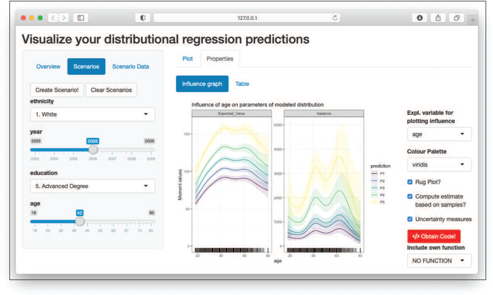
Influence of age on the first two moments of the predicted distributions for wage_model

Figure 6 shows the second main functionality of the interface, which is the ‘influence graph’ depicting the impact of a covariate on the first two moments based on the function plot_moments(). It appears after clicking the ‘Properties’ button and selecting the covariate of interest, in our case age. On the right side of the plot, numerous ways to customize it are provided. Clicking on the ‘Obtain Code’ button reveals a pop-up window displaying the R code needed to reproduce the graph. For a more comprehensive description of the GUI functionality, see Section B in the Appendix.

5 Discussion

This article laid out the foundations of Distributional Regression models and its implementations in R. It became clear that distributional regression provides a highly flexible modelling framework, from which researchers will increasingly benefit in the future. To make fitted models more accessible for users this article introduced the software distreg.vis based on the bamlss, gamlss and betareg R packages.

Using distreg.vis, the user can visualize predicted response distributions based on interactively chosen covariate combinations. Furthermore, distreg.vis provides the ability to show the influence of a selected explanatory covariate on the first two moments of any response variable, including continuous and discrete distributions. Both of these key functions help the user draw useful inference from fitted Bayesian and frequentist distributional regression models.

Moreover, distreg.vis is designed to be highly customizable. The user-specified covariate combinations (that represent the core of the analysis) can be individually edited and expanded. The graphical appearance of all plots can be changed to display other colour palettes or other distribution types (pdf/cdf). Succeeding the finished analysis, the user can obtain R code to reproduce the displayed plot with all chosen options.

With this new tool at hand, users will hopefully be more encouraged about applying distributional regression models and then draw more resilient conclusions. Nevertheless, further work on making distributional regression models more understandable can be done. The idea of visualizing predicted distributions and making influence plots could also be applied to other variations of distributional regression, for example BayesX (Brezger et al., 2005), VGAM (Yee, 2015) or GJRM (Marra and Radice, 2017), which offer a large variety of supported distributions.

Supplementary materials

Supplementary materials for this article including R codes and data are available at http://www.statmod.org/smij/archive.html.