
Abstract
We extend generalized additive models for location, scale and shape (GAMLSS) to regression with functional response. This allows us to simultaneously model point-wise mean curves, variances and other distributional parameters of the response in dependence of various scalar and functional covariate effects. In addition, the scope of distributions is extended beyond exponential families. The model is fitted via gradient boosting, which offers inherent model selection and is shown to be suitable for both complex model structures and highly auto-correlated response curves. This enables us to analyse bacterial growth in Escherichia coli in a complex interaction scenario, fruitfully extending usual growth models.
Introduction
In functional data analysis (Ramsay and Silverman, 2005), functional response regression aims at estimating covariate effects on response curves (Morris, 2015; Greven and Scheipl, 2017). The response curves might, for instance, be given by annual temperature curves, growth curves or spectroscopy data. We propose a flexible approach to regression with functional response allowing for simultaneously modelling multiple distributional characteristics of response curves following potentially non-Gaussian distribution families. It therefore generalizes usual functional mean regression models.
The problem of non-Gaussian functional response appears in many applications and is, accordingly, addressed in several publications. Following early works on non-Gaussian functional data by Hall et al. (2008) and van der Linde (2009), authors such as Goldsmith et al. (2015), Wang and Shi (2014) and Scheipl et al. (2016) proposed generalized linear mixed model (GLMM)’type regression models, which are suitable for, for example, positive, discrete or integer-valued response functions. The linear predictor for the mean function is typically composed of a covariate effect term and a latent random Gaussian error process accounting for auto-correlation, and combined with a link function. Li et al.(2014) jointly model continuous and binary-valued functional responses in a similar fashion, but without considering covariates. Other ideas to account for the auto-correlation of functional response curves include robust covariance estimation for valid inference after estimation under a working independence assumption (Gertheiss et al., 2015) and an overall regularization by early stopping a gradient boosting fitting procedure guided by curve-wise re-sampling methods as applied by (Brockhaus et al., 2015; Brockhaus et al., 2017) besides using curve-specific smooth errors. Moreover, this latter approach also offers quantile regression for functional data. The above approaches present important steps in generalizing functional regression models. In particular, our approach is a direct generalization of the framework of Brockhaus et al. (2015). However, the previous methods are restricted to one predictor such that none of them allows for simultaneously modelling also the response variance or other distributional parameters in a similar fashion as the mean. (Staicu et al., 2012) propose a method for estimating mean, variance and other shape parameter functions nonparametrically and also for non-Gaussian point-wise distributions, while modelling auto-correlation via copulas. However, they do not allow for including covariate effects. Only the framework of Scheipl et al. (2016) now allows to perform simultaneous mean and variance regression in the Gaussian case (Greven and Scheipl, 2017) and is also the only one currently offering a comparable range of smooth/linear effects of scalar and functional covariates, which are implemented in the R package
There are various approaches applied to modelling bacterial growth curves in the literature. Gompertz and Baranyi-Roberts models are two common parametric approaches to modelling growth curves (see, e.g., López et al., 2004; Perni et al., 2005). (Weber et al., 2014) implement a model particularly for analysing bacterial interaction. The models are usually fitted using least squares methods, which corresponds to assuming a Gaussian distribution of bacterial propagation. This is problematic as response values are naturally positive and very small in the beginning, starting from single cell level. Thus, also assuming a constant variance over the whole time span seems not appropriate. Moreover, they do not offer the opportunity to include covariate effects for modelling, for example, the impact of external factors. Thus, these models are not applicable here. In addition, they are often highly non-linear, which may introduce problems in parameter estimation. (Gasser et al., 1984) discuss this point and some further advantages of nonparametric growth curve regression over parametric models. They propose a kernel method for this purpose, which does, however, not include covariates and lacks the flexibility needed for our purposes. Still, non- or semi-parametric functional regression models present a natural choice from a statistical perspective, also because they can approximate the above parametric growth models very well when these are appropriate (Online Appendix E.2).
Besides providing the flexibility to meet all the challenges arising from the present analysis of bacterial interaction, we can show in extensive simulation studies that the presented approach is indeed well suited for complex scenarios with highly auto-correlated response curves despite working independence assumption: early stopping the gradient boosting algorithm based on curve-wise re-sampling techniques plays a key role in avoiding over-fitting and leads to highly improved estimation quality when comparing to the approach of (Greven and Scheipl, 2017).
The approach is implemented in the R (R Core Team, 2018) add-on package
The remainder of the article is structured as follows: In Section 2, we formulate the general model and describe the fitting algorithm. In Section 3, we apply the proposed model to analysing E. coli bacteria growth. Section 4 provides the results of two simulation studies for Gaussian response curves as well as for the growth model. Section 5 concludes with a discussion. Further details concerning the model, application and simulation studies are provided as Online Supplement, as well as the code for the simulations and fitting of the model with the R-package FDboost.
Model formulation
Consider a data scenario with
We assume that for all
where
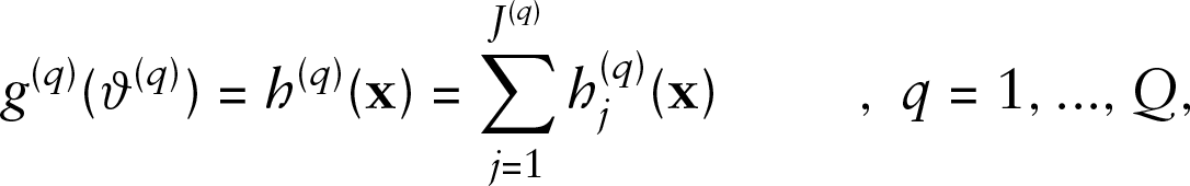
Both covariate and time dependency are modelled within the additive predictor via the effect functions
Overview of possible effect types (adapted from Brockhaus et al., 2015)
Overview of possible effect types (adapted from Brockhaus et al., 2015)
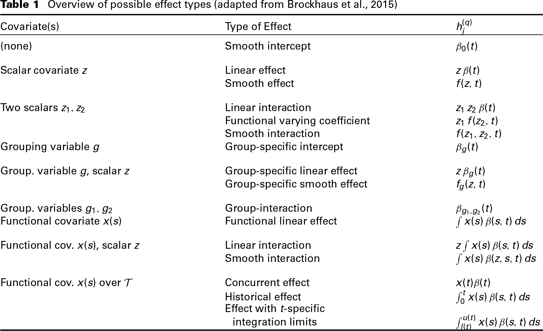
As both covariate and time dependency of the functional response are specified by the effect functions
For each effect type, 
A vector
A typical choice for
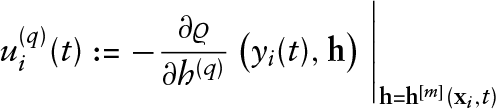
Component-wise gradient boosting is a gradient descend method for model fitting, where the model is iteratively updated. In each iteration, the algorithm aims at minimizing a loss function following the direction of its steepest descent. Instead of updating the full additive predictor at once, the individual effect functions
Let 
The functional GAMLSS loss function is then obtained as
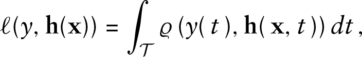
the integral over the point-wise loss functions over
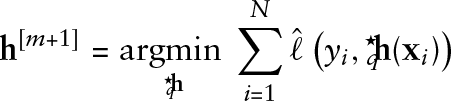
The aim of gradient boosting is to find the predictor

minimizing the expected loss.
Based on data 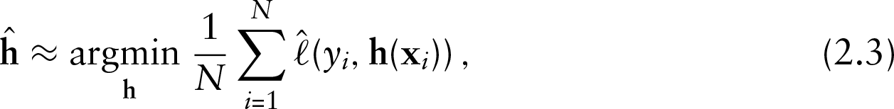
where
The minimization in (2.2) can be seen to minimize the Kullback–Leibler divergence (KLD) of the model density
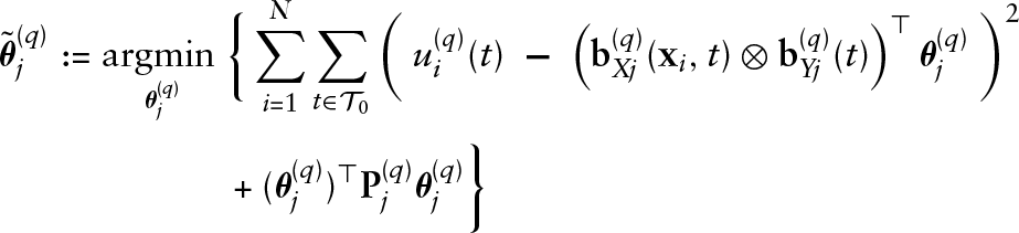
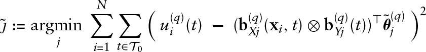
The base-learners fitted in each boosting iteration correspond to the effects
Algorithm: gradient boosting for functional GAMLSS
Initialize the coefficients
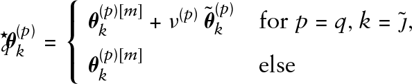
The smoothing parameters for the penalty matrices
The coexistence of various bacterial species is a key factor in environmental systems. Equilibria in this biodiversity stand or fall with the species’ interaction. Certain bacteria strains produce toxins and use them to assert themselves in bacterial competition. (von Bronk et al., 2017) establish an experimental set-up with two cohabiting Escherichia coli bacteria strains: a ‘C-strain’ producing the toxin ColicinE2 and a colicin sensitive ‘S-strain’ pipetted together on an agar surface. Single bacteria of the C-strain population sacrifice themselves in order to liberate colicin. The emitted colicin diffuses through the agar and kills numerous S-strain bacteria on contact. On the other hand, the S-strain might outgrow the C-strain and starts in a favoured position of an initial ratio S:C of about 100:1. The arising population dynamics are influenced by external stress induced with the antibiotic agent Mitomycin C (MitC). MitC slightly damages the DNA of the bacteria. While it has little effect on the S-strain, it triggers colicin production in the C-strain as an SOS-response. A higher dose of MitC increases the fraction of colicin producing C-bacteria and, thus, colicin emission (von Bronk et al., 2017).
At a total of
Model for S-strain growth
In order to obtain insights into bacterial interaction dynamics, we model the 
for
Results
MitC effect and effect of experimental batches
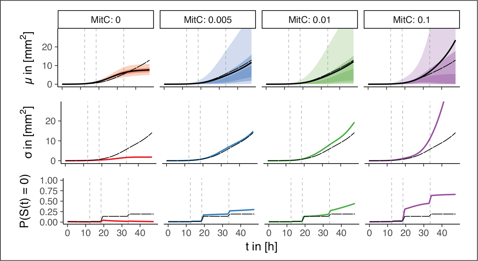
An overview of the effects of the toxin MitC can be found in Figure 1. We observe that mean S-strain growth is slightly increasing for low MitC levels compared to no MitC, but is particularly higher for
For the standard deviation, we observe a gradual but distinct rise with the MitC level. Due to the log-link we may not only interpret effects on the shape parameter
It is important to note, that control experiments indicate no considerable effect of MitC on S-strain growth (von Bronk et al., 2017). Thus, present covariate effects of MitC reflect effects of C-cells which cannot be explained by the observed C-strain growth curves. Showing distinct shifts at the zoom points,
The smooth functional effects for each of the eight experimental batches are relatively small in size. For the conditional mean
Estimated point-wise mean (top) and standard deviation (centre) of the S-strain growth curves
conditional on
and the extinction probabilities (bottom) of S-strain growth curves for each MitC concentration. Long-dashed curves correspond to the functional intercept, dashed vertical lines to the zoom level change-points. Thick solid lines indicate the estimates, transparent ribbons reflect the point-wise inner 25%, 50% and 90% probability mass intervals of the estimated gamma distributions conditional on
(top)
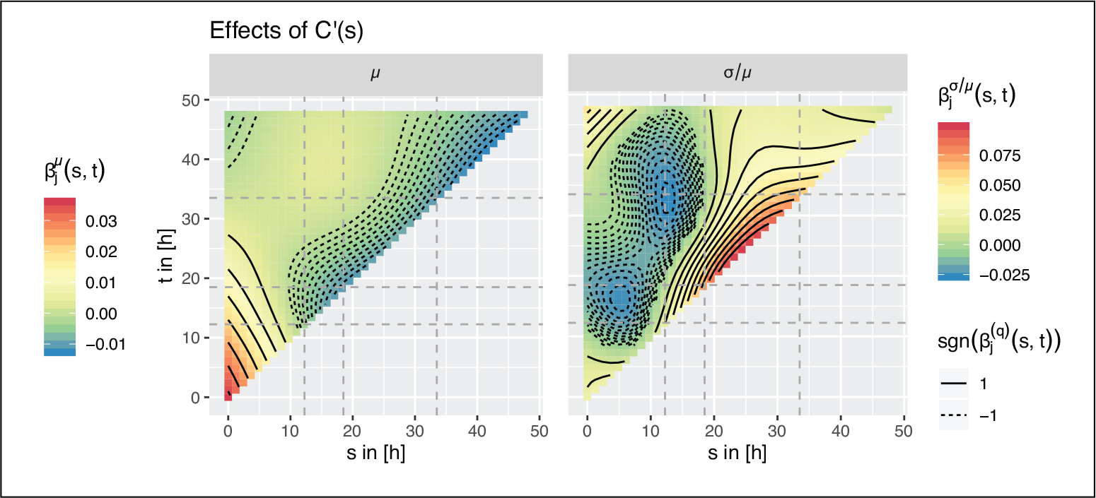
The base-learner for the C-strain area propagation
In the earlier growth phase with
In the second phase for
For the probability
Left: Coefficient function
for the historical effects of
on the mean of S-strain growth curves. Right: the corresponding plot for the effect of
on the scale parameter
. The
-axis represents the time line for the response curve, the
-axis represents the one for the C-strain growth curve. The change-points in zoom level are marked with dashed lines. For a fixed
,
and
describe the effect of the normalized covariate at time
on the S-strain growth curve over the whole remaining time interval.
Simulation set-up
Model-based gradient boosting approaches to non-functional or one-parameter special cases of the present model are well tested with respect to their fitting performance and variable selection quality (e.g., see Brockhaus et al., 2018a; Brockhaus et al., 2015; Thomas et al., 2018; Mayr et al., 2012) showing a typically slow over-fitting behaviour. However, modelling functional response variables with GAMLSS presents an important additional challenge: high auto-correlation in response functions may lead to severe over-fitting when estimating typically complex base-learners. While this is already the case for non-GAMLSS functional response models, it gets particularly acute for GAMLSS models with multiple predictors—if it is not properly controlled for by early stopping based on curve-wise re-sampling methods. We focus on this issue in an extensive simulation study investigating the fitting performance for different levels of in-curve dependency while also comparing different sample sizes, choices of hyper parameters, the non-cyclic and cyclic fitting method, and different (curve-wise) re-sampling methods. Moreover, we consider three different models in the simulation study: one model is directly based on the bacterial interaction scenario in Chapter 3 taking the model estimated on the original data as true underlying model; and two models with a Gaussian response distribution and categorical effects or more complex smooth (interaction) effects of metric covariates, respectively. There, we randomly generate different sets of true underlying effects in order to obtain as general results as possible. In the Gaussian case, where this is possible, we also compare to the penalized likelihood approach of (Greven and Scheipl, 2017) which is implemented in the R package
Simulation results
Considering the mean
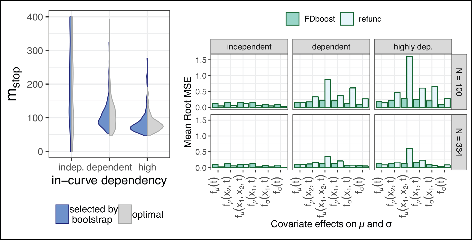
Plots referring to a Gaussian model scenario including smooth covariate effects
for
, the mean and standard deviation over time
, and for two metric covariates
, and a smooth interaction
effect for
(200 model fits per combination of sample size
and in-curve dependency level). Left: Violin-plots reflecting the empirical density of the stopping iterations
selected via 10-fold bootstrap (left) and for the
-optimal
(right) for
sampled curves. Right: Bar-plots indicating the mean RMSE of the different effects for our approach based on gradient boosting (FDboost , dark) and the approach based on penalized likelihood (refund , light). The highly dependent setting is the most realistic in many functional data scenarios and is—as far as the analogy can be drawn—the closest to the correlation structure in our application.
In the application motivated simulation scenario, we observe that most of the RMSEs for the estimated covariate effects are lower than 10% of the effect range even in the highly dependent setting (Online Appendix Figure 12). Exceptions are the functional intercept in the predictor for the extinction probability
The functional GAMLSS regression framework we present in this article allows for very flexible modelling of functional responses. We may simultaneously model multiple parameters of functional response distributions in dependence of time and covariates, specifying a separate additive predictor for each parameter function. In addition, point-wise distributions for the response curves beyond exponential family distributions can be specified. Doing so a vast variety of new data scenarios can be modelled. These new possibilities have shown to be crucial, when applying the framework to analyse growth curves in the present bacterial interaction scenario.
The results we obtain confirm and extend previous work: Focusing on the outcome after 48 hour and on the number of C-clusters at the edge of the S-colony after 12 hour, (von Bronk et al., 2017) already identify a phase of ’stochastic toxin dynamics’ followed by a phase of ’deterministic dynamics’ similar to the two phases of bacterial interaction we find in the historical functional effects of the C-strain growth. The functional regression model not only provides new evidence for this distinction from a completely new perspective, but now also allows to quantitatively discuss the effect of the C-strain on the S-strain over the whole time range: We now observe C-growth to have a positive effect on S-growth in the early phase and a negative effect in the later phase. The separation of these two phases appears even more distinct in the effect on the relative standard deviation, which we would not be able to recognize without GAMLSS.
Regarding the fraction of S- and C-strain area after 48 hour (von Bronk et al., 2017) categorized three different states of the bacterial interaction: for no MitC, there is either dominance of the S-strain or coexistence; for a moderate MitC concentration, there occurs a splitting into two extremes—either dominance of the S-strain or extinction; and for the highest MitC concentration, the toxin strategy of the C-strain fails and the S-strain either dominates or both strains go extinct. Now, referring to the complete growth curves, our results also reflect this categorization: If MitC is added, and conditional on a positive area, the mean S-strain growth increases, whereas also the probability for zero area and the variance increase. However, these differences would not be captured by non-GAMLSS regression models for the mean only, as the mean growth curves not conditioning on the response being positive are very similar for no and moderate MitC concentration (see Online Appendix Figure 17). Apart from that, the framework provides the flexibility to account for special challenges in the experimental set-up, such as dependencies between observations in the same experimental batch and differences between zoom levels of the microscope.
In simulation studies, we confirm that by fitting our models via component-wise gradient boosting we are capable of estimating even complex covariate effects on multiple distributional parameter functions. As it prevents over-fitting, early stopping of the boosting algorithm based on curve-wise re-sampling plays a key role: It enables us to face settings with highly auto-correlated response curves without explicitly modelling the correlation structure.
Supplementary material
Supplementary material including an Online Appendix with further details and illustrations, as well as R code and data used for the analysis of bacterial interaction and simulations is available from
Footnotes
Declaration of conflicting interests
Funding
Financial support from the Deutsche Forschungsgemeinschaft (DFG) through Emmy Noether grant GR 3793/1-1 (AS, SB, SG) and through grant OP252/4-2 part of the DFG Priority Program SPP1617 is gratefully acknowledged. B.v.B was supported by a DFG Fellowship through the Graduate School of Quantitative Biosciences Munich (QBM). Additional financial support by the Center for Nanoscience (CeNS) and the Nano Systems Initiative - Munich (NIM) is gratefully acknowledged.