Sage Journals: Discover world-class research

Abstract

The evolution of statistical modelling has historically been constrained by the practical limitations of computation; early statistical modelling favoured models which could feasibly be estimated. As increased mathematical complexity often implies more intricate computation, statistical models have grown both mathematically and computationally more complex. However, paradoxically, sometimes conceptually simpler models present more computational challenges than complex ones, and these have historically been neglected. In the case of binary responses, logistic regression models are the gold standard; covariates are modelled additively on the log-odds scale. In the case of time-to-event responses, the Cox proportional hazards regression model has additivity on the log-hazard rate scale. Both of these methods are computationally convenient, and yet the scales on which covariates are modelled are far from intuitive. We demonstrate the use of alternative models which are computationally more complex, yet feasible, but in which modelling is on a more interpretable scale. In the case of binary responses, a more intuitive alternative is log-binomial regression, in which modelling is on the log-relative risk scale. In the case of time-to-event responses, distributional regression enables modelling on the time scale. While logistic regression and proportional hazards regression qualitatively both deliver the same conclusions as the alternative models, log-binomial and distributional regression provide more interpretable coefficients, which are readily estimated.

Keywords

distributional regression logistic regression relative risk regression proportional hazards regression Cox model

1 Background

Statistical models are necessarily abstractions of the real world (‘All models are wrong’; Box, 1979). In the physical sciences, the abstraction may be rather close to reality, when the phenomenon under study is well understood; in other areas such as social sciences, the abstraction may be more speculative. In all cases, we observe data and formulate a statistical model to describe the data-generating mechanism, which is a mathematical abstraction of the real process.

When the purpose of the modelling is for prediction, the model’s predictive ability is all that matters. Interpretability is not important, and in fact the model may be a ‘black box’ (as in machine learning). However, when the purpose of the modelling is exploratory or confirmatory, whatever the extent of the abstraction, it is generally accepted that the model should be as simple as possible while retaining interpretability and usefulness.

Before going further, we need to define what we understand by ‘simple’, and to do this we distinguish between simplicity and mathematical convenience. By simplicity we mean closeness to the truth of the data or the evidence. For example, consider that we observe occurrences of a binary event. The most natural summary is the relative frequency, interpreted as a probability. Our contention is that this is as close as we can get to the evidence; and because it is close to the data, it is easily interpreted. We therefore regard the relative frequency or probability as a simple abstraction of the data. Another commonly used summary of such data is the odds, defined as the relative frequency of occurrences to non-occurrences. This is not an intuitive concept, yet because of its mathematical convenience (discussed below), it is ubiquitous in the analysis of binary and categorical data. Despite the mathematical and computational convenience of statistical models for the odds, the odds is a complex abstraction of the data.

1.1 Binary outcomes

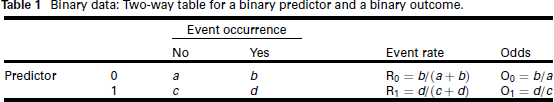
We consider the simplest situation of modelling a binary outcome as a function of a binary predictor (or risk factor or exposure or treatment allocation). The predictor at level 0 generally means the risk factor or exposure is absent or the treatment allocation is to control; 1 means presence or active treatment. Standard notation and terminology are given in Table 1.

Table 1

Binary data: Two-way table for a binary predictor and a binary outcome.

		Event occurrence
		No	Yes	Event rate	Odds
Predictor	0	a	b	$R_{0} = b / (a + b)$	$O_{0} = b / a$
	1	c	d	$R_{1} = d / (c + d)$	$O_{1} = d / c$

The event rates R₀ and R₁, for the predictor at levels 0 and 1, respectively, are alternatively referred to as risks of the event. To quantify the discrepancy between the event rates, two natural extensions are to define relative risk and risk difference:

relative risk: $RR = \frac{R_{1}}{R_{0}} = \frac{d / (c + d)}{b / (a + b)}$

risk difference: $RD = R_{1} - R_{0} = d / (c + d) - b / (a + b)$

both of which are intuitive quantities, in that, for example, a doubling of risk or a risk difference of 10% are concepts close to the data and unlikely to be misinterpreted. Clearly RR = 1, or equivalently RD = 0, indicate no difference in the risk for the predictor present or absent; there are simple statistical tests for this hypothesis.

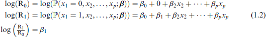
We would generally want to extend the analysis of Table 1 to include multiple predictors, that is, multiple regression with a binary outcome. This will enable quantification of risk, after adjustment for covariates. Clearly the appropriate response distribution is the Bernoulli, in which the probability parameter π is modelled with covariates:

\begin{matrix} y_{i} ∣ x_{i} \sim Bernoulli (π_{i}) \\ \begin{matrix} g (π_{i}) = g (π (x_{i}; β)) = x_{i}^{⊤} β & for i = 1, \dots, n \end{matrix} \end{matrix}

(1.1)

where $x_{i} = {(1, x_{i 1}, \dots, x_{i p})}^{⊤}$ is the covariate vector, $β = {(β_{0}, β_{1}, \dots, β_{p})}^{⊤}$ is the corresponding vector of coefficients, and g(.) is a suitable, monotonic, link function which determines the shape of the relationship between the parameter π and the linear predictor $x^{⊤} β$ . Choice of g(.) is central to the interpretation of the covariate effects on $p$ . We assume, without loss of generality, that $x_{1}$ is a binary covariate, for which we wish to determine the risk, adjusted for covariates $x_{2}, \dots, x_{p}$ . Let $R_{k} =$ $ℙ (x_{1} = k, x_{2}, \dots, x_{p}; β)$ for k = 0,1. We now define two alternative binomial regression models:

Relative risk regression model: $g (π) = log (π)$ .

\begin{array}{l} log (R_{0}) = log (ℙ (x_{1} = 0, x_{2}, \dots, x_{p}; β)) = β_{0} + 0 + β_{2} x_{2} + \dots + β_{p} x_{p} \\ log (R_{1}) = log (ℙ (x_{1} = 1, x_{2}, \dots, x_{p}; β)) = β_{0} + 1 + β_{2} x_{2} + \dots + β_{p} x_{p} \\ log (\frac{R_{1}}{R_{0}}) = β_{1} \end{array}

(1.2)

and $exp (β_{1}) = \frac{R_{1}}{R_{0}}$ is the adjusted relative risk for $x_{1}$ . (Similarly, for a continuous covariate $x_{j}$ , $exp (β_{j})$ is the adjusted relative risk for a 1-unit increase in $x_{j}$ .)

Risk difference regression model: $g (π) = π$ .

Similar mathematical reasoning as above shows that $β_{1}$ is the adjusted risk difference for $x_{1}$ . (Similarly, for a continuous covariate $x_{j}, β_{j}$ is the adjusted risk difference for a 1-unit increase in $x_{j}$ .)

So by varying the link function g(.), we easily define regressions on the scale of relative risk and risk difference. Yet these regressions are infrequently used in the analysis of binary data. Estimation of the relative risk and risk difference regression models poses problems due to the fact that the log and identity link functions do not guarantee constraint of the fitted values $\hat{π}$ to (0,1). For valid probability estimates, we require

\begin{matrix} {\hat{π}}_{i} = g^{- 1} (x_{i}^{⊤} \hat{β}) \in (0, 1) for i = 1, \dots, n . \end{matrix}

(1.3)

When the inverse of the link function, $g^{- 1} (\cdot)$ , is a sigmoid function, then (1.3) is automatically satisfied. This is always the case for the canonical link function; it is not the case for either the log or identity functions, with the result that solutions for (1.1) may produce invalid probability estimates in these cases. In the case of relative risk regression, this is overcome by the use of constrained optimization for maximisation of the likelihood of model (1.1). While this is intricate, the problems have largely been solved, using combinatorial EM-type algorithms and an adaptive barrier approach which achieve stable convergence (Donoghoe & Marschner, 2018). Similarly, a stable computational method for risk difference regression, which uses an equivalent additive Poisson formulation to arrive at a feasible MLE, is given by Donoghoe & Marschner (2014).

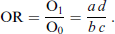
Another statistic shown in Table 1 is the odds, defined as O₀ and O₁ for the predictor at levels 0 and 1, respectively. To quantify the discrepancy between these, the odds ratio is used:

OR = \frac{O_{1}}{O_{0}} = \frac{a d}{b c} .

Much better known for the analysis of binary outcomes is logistic regression, which is based on the logistic link function, giving effects on the odds:

Logistic regression model:

\begin{matrix} g (π) = log \frac{π}{1 - π} . \end{matrix}

(1.4)

We define the adjusted odds for 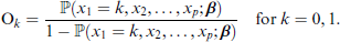$x_{1} = k$ as

O_{k} = \frac{ℙ (x_{1} = k, x_{2}, \dots, x_{p}; β)}{1 - ℙ (x_{1} = k, x_{2}, \dots, x_{p}; β)} for k = 0, 1.

Then use of the link function (1.4) in model (1.1), and similar mathematical reasoning as (1.2) yields

log (\frac{O_{1}}{O_{0}}) = β_{1}

and $exp (β_{1}) = \frac{O_{1}}{O_{0}}$ is the adjusted odds ratio for $x_{1}$ .

As is well known, the logistic link function is the canonical link for the Bernoulli distribution, so importantly delivers estimates $\hat{π} \in (0, 1)$ . Computation of MLEs is straightforward; logistic regression is available in all statistical software packages and is the go-to method for binary outcome data. However the odds scale for regression effects is far less intuitive than relative risk, discussed by multiple authors (e.g., Knol et al., 2011). OR and RR are approximately equal when R₀ is close to zero, or when RR < 1. However when RR > 1 and R₀ is not close to zero, OR exceeds RR, increasingly so as R₀ increases. So, for example, when R₀ = 0.4 and R₁ = 0.8, RR = 2 and OR = 6. While both measures indicate a substantial increase in risk and would lead to qualitatively the same conclusion, OR = 6 is a far more alarming statistic than RR = 2, being understood as ’six times the risk'. In general, the use of logistic regression will lead to qualitatively the same conclusions as relative risk and risk difference regression, so in that sense, its results are not misleading, but they are misleading if the quantification of the increase in risk is important. In summary, logistic regression is mathematically and computationally convenient, but is a complex abstraction of the data.

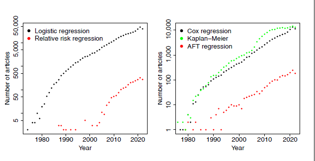
The left panel of Figure 1 shows the results of a search on PubMed Central of the terms ‘logistic regression’ and (‘relative risk regression’ or ‘log-binomial regression’ or ‘log binomial regression’), confirming the ubiquitous use of logistic regression, despite its interpretational difficulties discussed above, and the far more sparse use of relative risk regression.

Figure 1

Number of journal articles on PubMed Central containing the search terms. Left panel: ‘logistic regression’ and (‘relative risk regression’ or ‘log-binomial regression’ or ‘log binomial regression’). Risk difference regression has been omitted as very few instances were found. Right panel: (‘proportional hazards regression’ or ‘cox regression’), ‘Kaplan-Meier’ and (‘accelerated failure time’ or ‘parametric survival’). The y-axes are on the log scale.

1.2 Time-to-event outcomes

Time-to-event or survival outcomes have the typical feature of right-censoring, due to subjects either leaving the study or the study ending before observation of the event of interest. The simplest summary of the data, analogous to the computation of risks for binary data, is the estimated survival function, typically plotted as the Kaplan-Meier (KM) survival curve. This involves a relatively straightforward computation of the sample probability of survival over time, dependent on the number of subjects at risk at any time point.

Proceeding to the next level of analysis, we incorporate multiple predictors into a model for survival time. A natural approach is a regression model for time to event t; were it not for the censoring issue, a GLM-like multiple regression model could look like

\begin{matrix} t_{i} ∣ x_{i} \sim D (μ_{i}, σ); l o g (μ_{i}) = x_{i}^{⊤} β \end{matrix}

(1.5)

where $D (μ, σ)$ denotes a distribution with support on the positive real line; μ is a location parameter; σ is a scale/dispersion parameter; and the coefficients $β_{j}$ are additive effects on $log (μ)$ . Likelihood maximization for such models is straightforward; with censoring, estimation is somewhat more complicated, but generally feasible.

The development of regression models and the ability to perform complex iterative computations were limited until the early 1970s, when the seminal paper by Nelder & Wedderburn (1972) introduced generalized linear models. These would have gone part of the way to solving (1.5); however, this is not the trajectory that the analysis of survival data took. The closest model to (1.5) in the survival field is the accelerated failure time model (AFT):

\begin{matrix} log (t_{i}) = x_{i}^{⊤} β + ϵ_{i} \end{matrix}

(1.6)

where $ϵ_{i} \sim D^{*} (0, σ)$ is a parametric distribution with support on the real line. Commonly used choices for $D^{*}$ are the normal, logistic and extreme value (Gumbel) distributions, which imply lognormal, log-logistic and Weibull regression models for survival time t, respectively. (The standard Gumbel (0, 1) distribution for $D^{*}$ implies the exponential distribution for t.) The AFT model was first proposed by Pike (1966) and has been used primarily in the fields of reliability analysis (Newby, 1988) and medicine (Wei, 1992).

While this parametric approach to the modelling of survival time seems to be a natural one, historically things took quite a different turn. The ubiquitous approach to the modelling of survival data is the well-known proportional hazards (PH or Cox) model (Cox, 1972):

\begin{matrix} h_{i} (t) = h_{0} (t) exp (x_{i}^{⊤} β) \end{matrix}

(1.7)

where the hazard function h(t) is the instantaneous probability of an event at time t, conditional on survival to time $t; h_{0} (t)$ is the 'baseline hazard function', which is modified in (1.7) by the factor $exp (x_{i}^{⊤} β)$ to get the hazard function for subject i; and $exp (β_{j})$ are multiplicative effects on the hazard function. The regression model (1.7) does not make any assumption regarding the distribution of the time to event; however, implicit in (1.7) is the assumption that the hazard function has the same shape for all subjects ('proportional hazards').

The PH model (1.7) is very familiar to most statisticians; it is the go-to method for the analysis of survival data. And yet we contend that regression model (1.5) is a far more natural way of thinking about and modelling such data: survival time is observed, and effects on the mean or median survival time are simple and intuitive concepts. The hazard function, on the other hand, is not observed. It is a modelling abstraction and effects on it are, in the authors' experience, not well understood by applied researchers.

To understand why a less-obvious model has come to dominate the field, we need to look at the history of survival analysis. In a wide-ranging interview with Nancy Reid (1994), Sir David Cox explained that he had been approached by

Quite a few people ... said they were getting a certain kind of data, censored survival data, with a lot of explanatory variables. Nobody knew quite how to handle this sort of data in a reasonably general way, and there seemed to be dissatisfaction with assuming an underlying exponential distribution or Weibull distribution modified by some factor.

Cox developed the PH model in response, with the breakthrough being the separation of the likelihood into a part that involved $x_{i}^{⊤} β$ and the part that involved $h_{0} (t)$ , thus enabling maximization of the partial likelihood and avoiding estimation of $h_{0} (t)$ . This led to estimation which was feasible at the time and avoided the need to specify the response distribution.

So by 1972 there were two competing regression models for survival data: the AFT (1.6) and PH (1.7) models. The PH model completely eclipsed the AFT model in popularity, and continues to do so: Cox’s original paper (Cox, 1972) is ranked 24th in Nature’s list of most cited papers of all time in all fields (Van Noorden et al., 2014). Citations are in fact an underestimate of the popularity of the method: It has become so mainstream that generally papers in applications journals use the 'Cox model' without reference or with reference to a textbook. A better indicator of usage of the models is the number of journal articles using the terms 'Cox model' or 'proportional hazards model'. This is shown in the right panel of Figure 1, together with 'accelerated failure time models' and 'Kaplan-Meier' (obtained from PubMed searches). The pattern of PH vs AFT models is strikingly similar to logistic vs relative risk regression, albeit on a smaller scale. Note that Meier is even more widely used (according to this measure) than the PH model.

Sir David Cox was equivocal about the proliferation of his method. When asked about how he felt about the 'cottage industry that’s grown up around it' (Reid, 1994), Cox replied:

Don't know, really. In the light of some of the further results one knows since, I think I would normally want to tackle problems parametrically, so I would take the underlying hazard to be a Weibull or something. I'm not keen on nonparametric formulations usually ... if you want to do things like predict the outcome for a particular patient, it’s much more convenient to do that parametrically ... another issue is the physical or substantive basis for the proportional hazards model. I think that’s one of its weaknesses, that accelerated life models are in many ways more appealing because of their quite direct physical interpretation.

The AFT model (1.6) was developed in parallel to the GLM, and while it goes part of the way to addressing the specialized modelling needed for time-to-event outcomes, more general formulations are now possible. Following (1.5), we specify a distributional regression (or Generalized Additive Models for Location, Scale and Shape, GAMLSS) model (Stasinopoulos et al., 2024):

\begin{matrix} t_{i} ∣ x_{i} \sim D (θ_{i 1}, \dots, θ_{i K}) & for i = 1, \dots, n \\ g_{k} (θ_{i k}) = x_{i k}^{⊤} β_{k} & k = 1, \dots, K \end{matrix}

(1.8)

where $D (θ_{1}, \dots, θ_{K})$ is a K-parametric distribution with support on the positive real line; the $g_{k} (\cdot)$ are appropriate link functions; $θ_{1}$ (or μ) is a location parameter; and $θ_{2}, \dots, θ_{K}$ are shape or scale parameters. The main advantages of the distributional regression model (1.8) over the AFT model are the large number of distributions available for modelling (in current software, see below), the ability to model not just the location of the time distribution but also its shape, and the availability of complex additive terms (e.g., smoothing splines, random effects, spatial effects) in the linear predictors. Reviews of distributional regression are given by Kneib et al. (2023) and Hohberg et al. (2020), and demonstration of its usefulness in the clinical trials context by Heller et al. (2022). GAMLSS models are implemented in R in the maximum likelihood paradigm (gamlss; Stasinopoulos & Rigby, 2007), the Bayesian paradigm (bamlss; Umlauf et al., 2021) and the boosting paradigm (gamboostLSS; Thomas et al., 2018). For time-to-event analysis, right censoring can readily be accommodated in the likelihood.

Parametric models typically model the location of the survival time distribution, as well as possibly one or more shape parameters. In the case of heavy right censoring, they cannot reasonably be expected to estimate the central tendency accurately, when the central portion and upper tail of the distribution are unobserved. In this case, it makes sense to model the observed data, that is, the left tail. Quantile regression, another member of the distributional regression family, is useful in this context, in which we model the lower quantiles of the survival time distribution using censored quantile regression (Koenker, 2008), implemented in the R package quantreg (Koenker, 2023).

2 Application: Head and neck cancer outcomes

2.1 HNcSCC data

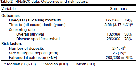
We analyse an observational study of n = 366 patients with head and neck cutaneous squamous cell carcinoma (HNcSCC) with regional metastases, treated between 1988 and 2020 (Hurrell et al., 2022). These patients typically have poor outcomes, and the purpose of this analysis is to identify predictive risk factors for mortality. The risk factors and outcomes we analyse are summarized in Table 2.

Table 2

HNcSCC data: Outcomes and risk factors.

Variable	Summary
Outcomes
Five-year (all-cause) mortality	179/366 = 49%
Time to (all-cause) death (years)	3.88 (3.17,461)^a
Censoring rate
Overall survival	132/366 = 36%
Disease-specific survival	286/366 = 78%
Risk factors
Number of deposits	2(1,4)^b
Size of largest deposit (mm)	26(15)^c
Extranodal extension (ENE)	288/366 = 79%

^a Median (95% CI). ^b Median (IQR). ^c Mean (SD).

2.2 Five-year mortality

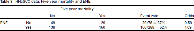
We begin with analysis of the binary outcome 'death within five years of diagnosis' (1 = dead; 0 = alive), and to keep things simple, we evaluate whether the binary factor extranodal extension (ENE, extension of tumour beyond the capsule of the lymph node into the surrounding tissue) is a significant risk factor. Table 3 gives the summary.

Table 3

HNcSCC data: Five-year mortality and ENE.

		Five-year mortality
		No	Yes	Event rate	Odds
ENE	No	49	29	29/78 = 37%	0.59
	Yes	138	150	150/288 = 52%	1.09

The relative risk for ENE is 1.40; the risk difference is 0.15 ; and the odds ratio is 1.84. Association between ENE and five-year mortality can be tested in a few ways: chi-square test: p = 0.027; z-test for log(RR) : p = 0.033; z-test for log (odds ratio): p = 0.020. Qualitatively, whichever statistic we compute and test, the conclusion regarding the significance of the association of ENE with five-year mortality is the same. However, if the magnitude of the effect matters, the odds ratio implies an 84% increase in "risk" (however that is understood), whereas relative risk shows a 40% increase and risk difference a 0.15 increase, much less alarming statistics.

The next level of complexity is to incorporate the other risk factors (number of deposits and size of largest deposit) into a multiple regression model for five-year mortality. We compare logistic regression with relative risk and risk difference regression.

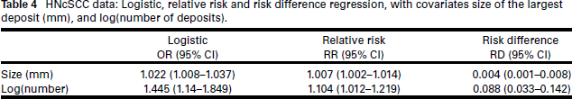
Variable selection was performed on the logistic regression model. As the number of covariates is only p = 3, the best-subsets method (Hastie et al., 2009) (effectively, enumeration) was used, with the BIC as the model selection criterion. All first-order interaction terms were considered for inclusion, making the number of models to be compared 18. Prior to performing the selection, it was determined that the appropriate form in the model for a number of deposits was logarithmic. (These workings are shown, for the simulated dataset, in the Supplementary Material.) The chosen covariates were size and log(number of deposits). For comparability, the same model was then used for the relative risk and risk difference regression models. Table 4 gives these results. We see a similar effect as above for ENE: while the predictors are significant in all models, the estimated odds ratios are far larger than the corresponding estimated relative risks.

Table 4

HNcSCC data: Logistic, relative risk and risk difference regression, with covariates size of the largest deposit (mm), and log(number of deposits).

	Logistic OR (95% CI)	Relative risk RR (95% CI)	Risk difference RD (95% CI)
Size (mm)	1.022 (1.008-1.037)	1.007 (1.002-1.014)	0.004 (0.001-0.008)
Log(number)	1.445 (1.14-1.849)	1.104 (1.012-1.219)	0.088 (0.033-0.142)

2.3 Survival

2.3.1 Overall survival

The KM curve for the HNcSCC overall survival is shown in the top left panel of Figure 2; fairly even mortality over the 16 -year study is evident.

Figure 2

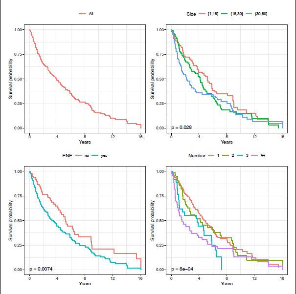
HNcSCC data: KM curves, by all (top left), size (top right), ENE (bottom left), and number of deposits (bottom right). P-values shown are for the log-rank test.

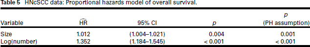
For consistency with the binomial regression models, we do not perform variable selection for the PH model; instead, we use the same predictors as were selected for the logistic regression model. Table 5 gives these results: size and log(number of deposits) are highly significant. However, the test of the PH assumption is strongly rejected for both covariates; this is confirmed graphically by the crossing of the survival curves for these two covariates in the KM plots (Figure 2, top right and bottom right panels). Although both appear to be important risk factors, we would be ill-advised to estimate their effects using a PH model.

Table 5

HNcSCC data: Proportional hazards model of overall survival.

Variable	$\hat{H R}$	95% Cl	p	p (PH assumption)
Size	1.012	(1.004-1.021)	0.004	0.001
Log(number)	1.352	(1.184-1.545)	< 0.001	< 0.001

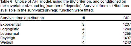
Moving to parametric models, we consider AFT and GAMLSS models. For the AFT model (1.6), survival time distributions considered were those available in the survival::survreg() function, viz., the exponential, loglogistic, lognormal, Rayleigh and Weibull. (In survreg(), the implied distribution for survival time t, rather than the distribution $D^{*}$ for $l o g (t)$ , is specified.)

Response distribution choice was conditioned on the covariates size and log(number of deposits) in (1.6). The exponential distribution for survival time is chosen on the basis of the BIC (Table 6), which implies the Gumbel(0, 1) distribution for the error term of the AFT model.

Table 6

Choice of AFT model, using the BIC criterion, and conditioned on the covariates size and log(number of deposits). Survival time distributions available in the survival::survreg() function were fitted.

Survival time distribution	df	BIC
Exponential	3	1237
Loglogistic	4	1240
Lognormal	4	1255
Rayleigh	3	1497
Weibull	4	1243

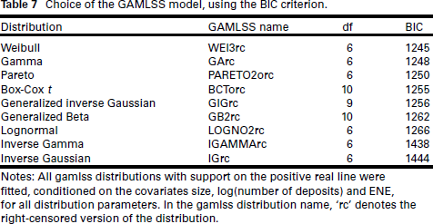
For the GAMLSS model (1.8), model selection is more complex, and we perform this without reference to the model selection of previous models. The first task is to select the response distribution: right-censored versions of all available distributions with support on the positive real line in the gamlss package were considered. Response distribution choice was conditioned on the covariates size, log(number of deposits) and ENE in the model equations for all distribution parameters $θ_{k}$ , in (1.8). Selection was made on the basis of the BIC, shown in Table 7. The Weibull distribution is chosen: this is the $V E I (μ, σ)$ parametrization, in which μ is the mean and σ is a shape parameter (Rigby et al., 2019).

Table 7

Choice of the GAMLSS model, using the BIC criterion.

Distribution	GAMLSS name	df	BIC
Weibull	WEI3rc	6	1245
Gamma	GArc	6	1248
Pareto	PARETO2orc	6	1250
Box-Cox t	BCTorc	10	1255
Generalized inverse Gaussian	GIGrc	9	1256
Generalized Beta	GB2rc	10	1262
Lognormal	LOGNO2rc	6	1266
Inverse Gamma	IGAMMArc	6	1438
Inverse Gaussian	IGrc	6	1444

Notes: All gamlss distributions with support on the positive real line were fitted, conditioned on the covariates size, log(number of deposits) and ENE, for all distribution parameters. In the gamlss distribution name, 'rc' denotes the right-censored version of the distribution.

We now proceed to variable selection. As the number of covariates is small, a variant of best-subset selection (Hastie et al., 2009) is used. Size, log(number of deposits), ENE and their first-order interactions are considered for both μ and σ. As for the variable selection performed for logistic regression, the number of models to be compared for a single distribution parameter is 18. With two distribution parameters μ and σ, the number of models to be compared is then 18². = 324. While this is feasible for this application, as p increases, this number will quickly blow out. We adopt the pragmatic method suggested by Stasinopoulos et al. (2024, Chapter 9): using best-subsets selection, first the model for μ is selected, conditional on a null model for σ; conditional on the chosen model for μ, the model for σ is selected; then the process is repeated. Size and log(number of deposits) are chosen for μ; and log(number of deposits) for σ. Formulations of both AFT and GAMLSS models are shown in (2.1).

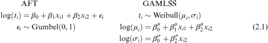
\begin{matrix} AFT & GAMLSS \\ log (t_{i}) = β_{0} + β_{1} x_{i 1} + β_{2} x_{i 2} + ϵ_{i} & t_{i} \sim Weibull (μ_{i}, σ_{i}) \\ ϵ_{i} \sim Gumbel (0, 1) & \log (μ_{i}) = β_{0}^{μ} + β_{1}^{μ} x_{i 1} + β_{2}^{μ} x_{i 2} \\ \log (σ_{i}) = β_{0}^{σ} + β_{2}^{σ} x_{i 2} \end{matrix}

(2.1)

where x₁ is the size of the largest deposit and x₂ is log(number of deposits).

Parameter estimates are given in Table 8. Noteworthy is the similarity between the PH, AFT and GAMLSS models: The covariates for the location parameter all point in the direction of increasing number and size of deposits being significantly detrimental to survival. In addition, in the GAMLSS model, log(number of deposits) also affects the shape parameter σ.

Table 8

HNcSCC data: Parametric models of overall survival: AFT exponential model and GAMLSS Weibull model.

Model	Variable	AFT, exponential		GAMLSS, Weibull
		$\hat{β} (SE)$	p	$\hat{β} (SE)$	p
μ	size	−0.014 (0.004)	0.001	−0.012 (0.004)	0.003
	log(number)	−0.305 (0.067)	0.000	−0.244 (0.081)	0.003
σ	log(number)	-	−0.147 (0.053)	0.006

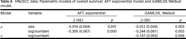
We contrast the information given on the effect of the size of the largest deposit on survival time by the three models. A 1 mm increase in size is associated with a 1.2% increase in the hazard rate (PH model), a 1.4% decrease in median survival time (AFT model) and a 1.2% decrease in mean survival time (GAMLSS model). While the messages from the three models are qualitatively the same, effects on mean or median survival are surely more accessible to applied researchers than effects on the hazard rate.

The effect of the number of deposits in the AFT model is reasonably straightforward. Because the predictor is log(number of deposits), the effect of a 100p% increase in number of deposits on median survival time is ${(1 + p)}^{β_{2}}$ : for example, the effect of a 10% increase in the number of deposits is 1.1^-0.305, = 0.971, a 2.9% decrease. In the GAMLSS model, however, the covariate appears in the equations for both μ and σ; as a result, it is not helpful looking at the effect of the number of deposits on, say, μ, because a change in the number of deposits affects both μ and σ, that is, it affects both the location and shape of the distribution. Instead, we examine the fitted survival time distributions over a range of values of the number of deposits, for a fixed value of size of largest deposit, to gauge the influence of number of deposits on the whole survival time distribution. Figure 3 shows this effect for the size of the largest deposit fixed at its mean of 26.4 mm. It is clear that a small number of deposits results in survival time distribution with less probability at the origin and more in the tail (i.e., longer survival, on average), whereas a larger number of deposits have the opposite effect with more at the origin and less in the tail.

Figure 3

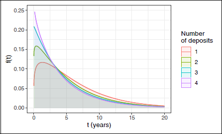
Distributional regression Weibull model for overall survival. Probability density functions of survival time by number of deposits, with size of the largest deposit fixed at its mean 26.4 mm.

2.3.2 Disease-specific survival

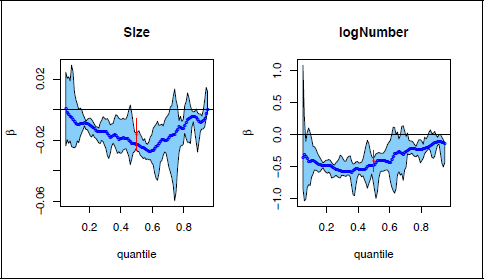
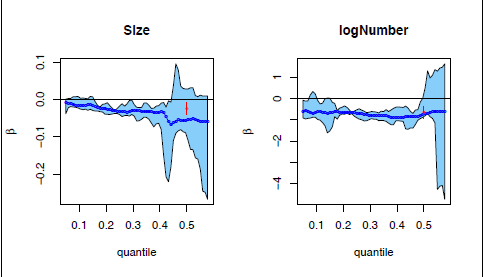
The censoring rate for disease-specific survival is high at 78% (cf. 36% for overall survival). While PH regression is feasible in this case, it is not very informative since estimates of the log hazard ratio will have low precision. Parametric regression models for the mean or median survival time will also not be useful as only the lower tail of the survival time distribution is observed. A distributional regression model that will provide reliable information in this scenario is censored quantile regression, estimated at the lower quantiles of the survival time distribution. We illustrate the use of censored quantile regression for disease-specific survival and overall survival. Figure 4 depicts the regression estimates and 95% confidence band for size of largest deposit and log(number of deposits), at quantiles in the range of 0-1, for the overall survival outcome. The left panel shows that size has the most effect on the distribution of overall survival in the centre (around the 0.6 quantile), and the least effect in the tails; the right panel shows the strong effect of log(number of deposits) in the lower tail and centre of the distribution, but not in the upper tail. The parametric estimates for the median (shown in red) were obtained from a model similar to the GAMLSS model in (2.1), but using the lognormal rather than the Weibull so that effects are on the median rather than the mean, for comparability with quantile regression. These estimates are fairly similar to the quantile regression estimates.

Figure 4

Censored quantile regression estimates for HNcSCC overall survival times. The blue lines and the light blue region give the censored quantile regression estimates and their $95 %$ confidence band; the red estimates and confidence intervals at the 0.5 quantile are for the median in corresponding parametric models.

For disease-specific survival, the quantile regression results are shown in Figure 5. As could have been expected, estimates above the 0.4 quantile are completely unreliable, and in fact could not be computed above the 0.6 quantile. However, below the 0.4 quantile the estimates appear to be stable and demonstrate a similar effect as in overall survival, viz., a harmful effect on survival of increasing size and number of deposits. The parametric estimates of the median severely underestimate the variability.

Figure 5

Censored quantile regression estimates for the lower tail of HNcSCC disease-specific times. The blue lines and the light blue region give the censored quantile regression estimates and their $95 %$ confidence band; the red estimates and confidence intervals at the 0.5 quantile are for the median in corresponding parametric models.

3 Discussion

Statistical methods which are entrenched as the standard for analysis may not necessarily be based on conceptually simple abstractions of the data-generating mechanism and may have gained acceptance due to their mathematical convenience or computational feasibility within the limits of computing power at the time they were developed. Logistic regression and proportional hazards regression both fall into this category. Odds ratios and hazard ratios deliver qualitatively the same information as more intuitive quantities such as relative risks and effects on the mean or median survival time, but quantitatively they are not well interpreted. We have demonstrated that under current computing capability, these simpler concepts are readily estimated.

For tumour outcomes, the timing of mortality is considered to be more important than the binary notion of 'dead/alive within X years', as this gives clinicians an understanding of tumour behaviour. In that sense, the survival analysis is of far more clinical interest than the analysis of five-year mortality; nevertheless, we have presented the latter for statistical interest. For HNcSCC, clinical interest is in the five years following diagnosis; however, we have analysed the survival data to their limit of 16 years post-diagnosis.

Survival data are structurally different from non-temporal outcomes, because of the temporal nature of the outcome and possibly the covariate(s). Regression modelling may be accomplished on different scales:

hazard function h(t) : PH (Cox) regression and its many variants

time t: AFT regression, distributional regression (GAMLSS, quantile regression)

survival function S(t): generalized survival models (Liu et al., 2018).

There is a very rich body of survival modelling based on the hazard function. While the hazard function is not observable and perhaps less well understood than the survival function, it is informative of the course of a disease (when estimated). PH regression has the ability to incorporate the important feature of time-varying covariates and time-varying coefficients. It is difficult to overstate the pervasive nature of the hazard function and proportional hazards concept in survival analysis; and almost impossible to find a discussion of time-to-event data without mention of the hazard function. The AFT model, on the other hand, is the sadly neglected 'poor relation' of survival analysis. And yet it was ahead of its time, foreshadowing the development of the rich framework of distributional regression models, which have superseded it.

We urge applied researchers to be mindful of the interpretability of their analyses, and as far as possible to model the observed outcome on a simple and intuitive scale. Models which historically may not have been computationally feasible are readily accessible in the rich framework provided by distributional regression and generalized linear models with non-canonical links.

Data and software

The HNcSCC dataset was extracted from the Sydney Head and Neck Cancer Institute (SHNCI) Database, which is currently housed at the Chris O'Brien Lifehouse, Sydney. The data are not available openly. R version 4.2.3 (R Core Team, 2023) was used; the packages logbin (Donoghoe & Marschner, 2018) and addreg (Donoghoe & Marschner, 2014) were used for the estimation of log-binomial and risk difference regression, respectively, for distributional regression, the packages gamlss (Stasinopoulos & Rigby, 2007) and quantreg (Koenker, 2008) were used.

Supplementary materials

All computations in this article are reproduced on a dataset simulated to have similar characteristics to the HNcSCC dataset. The supplementary materials include the analysis code and output and the simulated dataset. They are available from the journals page at https://journals.sagepub.com/home/smj.

Supplemental Material for Simple or complex statistical models: Non-traditional regression models with intuitive interpretations by Gillian Z. Heller, in Statistical Modelling

Footnotes

Acknowledgements

This work was presented as an invited talk at the 37th International Workshop on Statistical Modelling (IWSM) held in Dortmund, Germany, in 2023. The author thanks the IWSM organisers for their support; Professor Tsu-Hui (Hubert) Low of the Chris O'Brien Lifehouse, Sydney, and Sydney Medical School, Faculty of Medicine and Health, University of Sydney, for the provision of the HNcSCC data and clinical guidance; and Wilson Luna Guzman, database manager at SHNCI.

Declaration of Conflicting Interests

The author declared no potential conflicts of interest with respect to the research, authorship and/or publication of this article.

Funding

The author received no financial support for the research, authorship and/or publication of this article.

References

Box

GEP

(1979) Robustness in the strategy of scientific model building. Robustness in Statistics , 1, 201–36.

Cox

(1972) Regression models and life-tables. Journal of the Royal Statistical Society: Series B (Methodological) , 34(2), 187–202.

Donoghoe

and Marschner

(2014) Stable computational methods for additive binomial models with application to adjusted risk differences. Computational Statistics & Data Analysis , 80, 184–96. doi: 10.1016/j.csda.2014.06.019.

Donoghoe

and Marschner

(2018) logbin: an R package for relative risk regression using the log-binomial model. Journal of Statistical Software , 86, 1–22.

Hastie

, Tibshirani

and Friedman

(2009) The elements of statistical learning: data mining, inference and prediction . 2nd edition. New York: Springer.

Heller

, Robledo

and Marschner

(2022) Distributional regression in clinical trials: treatment effects on parameters other than the mean. BMC Medical Research Methodology , 22(1), 1–12.

Hohberg

, Pütz

and Kneib

(2020) Treatment effects beyond the mean using distributional regression: methods and guidance. PLOS ONE , 15(2), e0226514.

Hurrell

, Heller

, Elliott

, Gao

, Ebrahimi

, Clark

, Shannon

, Palme

, Wykes

, Gupta

, Ch'ng

, Nguyen

and T-H

Low

(2022) Recursive partitioning to determine order of significance of regional metastasis characteristics in head and neck cutaneous squamous cell carcinoma. Annals of Surgical Oncology , 29(11), 6991–99.

Kneib

, Silbersdorff

and Säfken

(2023) Rage against the mean - a review of distributional regression approaches. Econometrics and Statistics , 26, 99–123. https://doi.org/10.1016/j.ecosta.2021.07.006.

10.

Knol

, Duijnhoven

, Grobbee

, Moons

and Groenwold

(2011) Potential misinterpretation of treatment effects due to use of odds ratios and logistic regression in randomized controlled trials. PLoS One , 6(6), e21248.

11.

Koenker

(2008) Censored quantile regression redux. Journal of Statistical Software , 27, 1–25.

12.

Koenker

(2023) Quantreg: quantile regression . URL https://CRAN.R-project.org/package=quantreg. R package version 5.96.

13.

X-R

Liu

, Pawitan

and Clements

(2018) Parametric and penalized generalized survival models. Statistical Methods in Medical Research , 27(5), 1531–46.

14.

Nelder

and Wedderburn

(1972) Generalized linear models. Journal of the Royal Statistical Society: Series A (General) , 135(3), 370–84.

15.

Newby

(1988) Accelerated failure time models for reliability data analysis. Reliability Engineering & System Safety , 20(3), 187–97.

16.

Pike

(1966) A method of analysis of a certain class of experiments in carcinogenesis. Biometrics , 22(1), 142–61.

17.

Core Team

(2023) R: a language and environment for statistical computing. R Foundation for Statistical Computing, Vienna, Austria . URL https://www.R-project.org/.

18.

Reid

(1994) A conversation with Sir David Cox. Statistical Science , 9(3), 439–55.

19.

Rigby

, Stasinopoulos

, Heller

and De Bastiani

(2019) Distributions for modeling location, scale, and shape: using GAMLSS in R . Boca Raton: Chapman & Hall/CRC.

20.

Stasinopoulos

and Rigby

(2007) Generalized additive models for location, scale and shape (GAMLSS) in R. Journal of Statistical Software , 23(7), 1–46.

21.

Stasinopoulos

, Kneib

, Klein

, Mayr

and Heller

(2024) Generalized additive models for location, scale and shape: a distributional regression approach, with applications . Cambridge University Press.

22.

Thomas

, Mayr

, Bischl

, Schmid

, Smith

and Hofner

(2018) Gradient boosting for distributional regression: faster tuning and improved variable selection via noncyclical updates. Statistics and Computing , 28(3), 673–87. doi: 10.1007/s11222-017-9754-6.

23.

Umlauf

, Klein

, Simon

and Zeileis

(2021) bamlss: a Lego toolbox for flexible Bayesian regression (and beyond). Journal of Statistical Software , 100(4), 1–53. doi: 10.18637/jss.v100.i04.

24.

Van Noorden

, Maher

and Nuzzo

(2014) The top 100 papers. Nature News , 514(7524), 550.

25.

Wei

(1992) The accelerated failure time model: A useful alternative to the Cox regression model in survival analysis. Statistics in Medicine , 11(14-15), 1871–79. doi: https://doi.org/10.1002/sim.4780111409.

Supplementary Material

Please find the following supplemental material available below.

For Open Access articles published under a Creative Commons License, all supplemental material carries the same license as the article it is associated with.

For non-Open Access articles published, all supplemental material carries a non-exclusive license, and permission requests for re-use of supplemental material or any part of supplemental material shall be sent directly to the copyright owner as specified in the copyright notice associated with the article.

0.45 MB

0.00 MB