
Abstract
In online surveys, response time data are often used to make inferences about respondents’ cognitive processing of survey questions and to assess survey data quality. Adequate data preparation is crucial prior to analysis of response time data, in particular the detection and handling of outliers, which are extremely short or long response times. While several outlier detection methods exist, there is little empirical guidance on which method to use and how the choice affects response time data. We compared nine outlier detection methods commonly used in survey research across nine survey questions with varying characteristics, using data from a probability and a nonprobability online panel. Results show substantial differences between outlier detection methods in the proportion of outliers identified and in the effects of outlier exclusion on the response time data, with the effects being more pronounced in the nonprobability panel. Moreover, outlier detection methods differ systematically in the types of cases they classify as outliers, particularly with respect to respondent age and education. Based on these findings, recommendations for outlier detections methods in survey research are discussed.
Introduction
When it comes to the collection and use of paradata in survey research, response time data is among the most frequently examined and widely applied types of paradata. Particularly in online surveys, response times―the time a respondent takes to answer a survey question―are used for various methodological purposes that enhance our understanding of response behavior. They provide insight into the cognitive processing of survey questions and the quality of responses provided (e.g., Matjašic et al., 2018; Olson & Parkhurst, 2013). A key application is to assess the cognitive effort required to answer different types of questions, which helps identify items that may be too complex, ambiguous, or poorly designed. Response times also serve as indicators of respondent engagement and data quality, allowing researchers to detect suboptimal response behavior during or after data collection. In addition, response times serve as a valuable indicator for evaluating how different questionnaire and survey design features, such as the question format and design, the survey mode, or type of device used (e.g., desktop vs. smartphone), affect respondent behavior in general and across different groups. By comparing response time patterns across groups (e.g., younger vs. older respondents, or probability vs. nonprobability panelists), researchers can identify differential effects of design choices on cognitive effort, engagement, and potential data quality issues.
To draw meaningful conclusions from response time data, it is essential to clean the data prior to analysis―particularly by identifying and handling outliers. Response time outliers generally fall into two categories: extremely short and extremely long response times, which often arise from “processes that are not the ones being studied” (Ratcliff, 1993, p. 510). If left unaddressed, outliers can distort descriptive statistics (e.g., mean and standard deviation) and bias coefficient estimates. Moreover, high variability introduced by such extreme values can reduce statistical power and makes it more difficult to detect statistically significant differences—thereby increasing the risk of Type II errors (Fazio, 1990; Mulligan et al., 2003). Conversely, inappropriate handling or overly removal of outliers can artificially increase statistical power, potentially inflating Type I error rates and leading to spurious findings (Vankov, 2023).
While various techniques exist for identifying and handling response time outliers (for an overview, see Matjašic et al., 2018), little is known about how these methods compare in practice, particularly across different types of online panels. Only a few studies have systematically examined the consequences of different outlier detection methods for the resulting response time data (e.g., Berger & Kiefer, 2021; Höhne & Schlosser, 2018; Stocké, 2004). To the best of our knowledge, no research has explored how these methods perform across different panel types, including probability and nonprobability online panels. Additionally, no research has examined whether different outlier detection methods systematically identify certain respondent groups, and if the patterns vary by panel type.
The present study contributes to the literature by providing a systematic comparison of response time outlier detection methods across probability and nonprobability online panels. By applying multiple commonly used detection methods to the same survey questions administered in both panels, we examined whether the choice of method had differential consequences for the identification of outliers and the characteristics of response time data depending on the panel type. In addition, we investigated how the detection methods differed in identifying certain groups of respondents as outliers in both panels. Our study is guided by the following research questions: RQ1: How do outlier detection methods differ in their effects on response time data between probability and nonprobability online panels? RQ2: Do outlier detection methods differ in terms of which respondent groups are identified as response time outliers between probability and nonprobability online panels?
Background
Processing of Survey Questions
Respondents typically engage in a multi-stage cognitive process to properly understand survey questions and provide high-quality responses (e.g., Groves, 1989; Jenkins & Dillman, 1997; Sudman et al., 1996; Tourangeau et al., 2000). However, rather than working conscientiously through each stage to provide an optimal response, respondents may skip one or more stages and satisfice to minimize cognitive effort (Krosnick, 1991). Very short response times may indicate satisficing, while longer times may suggest deeper processing (Bowling et al., 2023; Callegaro et al., 2009; Dustin et al., 2017; Höhne et al., 2017; Lenzner et al., 2010; Toepoel et al., 2008). However, excessively long response times can also signal difficulties processing questions (e.g., Christian et al., 2009; Couper et al., 2006; Funke et al., 2011; Horwitz et al., 2017), or multitasking, which means that respondents do something else while answering the questions, or even interrupt the survey and come back later (Ansolabehere & Schaffner, 2015; Höhne et al., 2020; Sendelbah et al., 2016). Therefore, both fast and slow response times can be indicative of inattentiveness and satisficing (Read et al., 2022).
Factors Affecting Response Time
Factors affecting response times are manifold. Broadly, they can be categorized according to (a) respondent characteristics such as gender, age, and education; (b) questionnaire characteristics such as question type and complexity; and (c) survey design features or contextual factors relating to the environment in which the survey is conducted (e.g., Andreadis, 2015; Yan & Tourangeau, 2008). Although this categorization simplifies the complex set of influencing factors and does not cover all of them, it does include some of the key variables that previous studies have shown to influence response times. Furthermore, these variables are generally available in surveys without requiring additional data collection and thus offer practical value for widespread application in survey research.
Concerning respondent characteristics, previous research showed that older respondents tend to have longer response times, possibly due to slower reading speed, reduced working memory capacity, reduced familiarity with digital interfaces, or more careful processing (Gummer & Roßmann, 2015; Yan & Tourangeau, 2008). Similarly, those with lower education levels spend more time answering survey questions (Andreadis, 2015; Couper & Kreuter, 2013; Gummer & Roßmann, 2015; Shi et al., 2018; Yan & Tourangeau, 2008). Female respondents spend more time than male (Andreadis, 2015; Shi et al., 2018).
Relating to questionnaire characteristics, studies have shown that attitudinal questions tend to take longer to complete than factual questions, presumably because attitudinal responses require more difficult retrieval and integration (Bassili & Fletcher, 1991; Schneider et al., 2023; Yan & Tourangeau, 2008). Cognitively complex questions that are more difficult to answer also need more time (Couper & Kreuter, 2013; Garbarski et al., 2020; Horwitz et al., 2017; Leipold et al., 2024). In line with this, open-ended questions take longer than other types of questions as they require retrieval, formulation, and typing (Couper & Kreuter, 2013; Gummer & Roßmann, 2015).
Regarding survey design features and contextual factors, previous studies have generally found that respondents using smartphones take longer to complete questions than those using desktops (Andreadis, 2015; Antoun et al., 2017; Décieux & Sischka, 2024; Gummer & Roßmann, 2015), while other studies have found no such difference (Revilla & Couper, 2018). In general, longer response times are attributed to smaller screen sizes and touch input limitations, as well as increased cognitive load from scrolling or navigating complex layouts, so using a mobile-friendly layout may help mitigate differences between smartphone and desktop respondents. Moreover, nonprobability panelists are considered more prone to satisficing due to self-selection, frequent survey invitations, and incentive-driven participation (Baker et al., 2010; Cornesse & Blom, 2023; Greszki et al., 2014; Hillygus et al., 2014; Matthijsse et al., 2015). Although nonprobability panelists are likely to take less time to answer or even speed through surveys more often, studies show this does not necessarily equate to lower response quality (Greszki et al., 2014; Gummer & Roßmann, 2015; Hillygus et al., 2014; Keusch et al., 2014; Matthijsse et al., 2015; Zhang et al., 2020).
Methods for Detecting Response Time Outliers
Looking at previous survey methodological studies that analyzed response times, there are a variety of different techniques for identifying and dealing with response time outliers (for an overview, see Leys et al., 2013; Matjašic et al., 2018; Rousseeuw & Hubert, 2011).
Cut-Off Values and Percentiles
Outliers are defined by setting fixed cut-off thresholds, with percentiles often serving as cut-off values (e.g., 95th or 99th percentile). Percentile methods are widely used in survey research to identify values at the extremes of the response time distribution, either on the upper end alone (e.g., Antoun & Cernat, 2020; Couper & Peterson, 2017; Mavletova, 2013; Neuert et al., 2024; Revilla & Ochoa, 2015; Tijdens, 2014; Yan et al., 2010) or on both ends (e.g., Gummer & Roßmann, 2015; Harms et al., 2017; Höhne et al., 2020; Kaczmirek, 2009; Lenzner et al., 2010; Revilla & Couper, 2018; Revilla et al., 2020; Yan & Tourangeau, 2008). Absolute cut-off values (e.g., 30 minutes or 5 seconds) are also applied, but they risk ignoring data distribution, which can lead to arbitrary classifications (e.g., Tourangeau et al., 2004, 2007; Callegaro et al., 2009; Couper & Zhang, 2016; Healey, 2007; Husser & Fernandez, 2013; Knowles & Condon, 1999).
Means and Standard Deviation
Another common approach in survey research defines outliers as values falling beyond a set number of standard deviations (e.g., mean ± 2 or 3 SD) from the mean (e.g., Bauer et al., 2025; Christian et al., 2009; Heerwegh & Loosveldt, 2006; Kunz & Meitinger, 2022; Mahon-Haft & Dillman, 2010; Malhotra, 2008; Naemi et al., 2009; Smyth et al., 2009; Toepoel et al., 2008). This method assumes normal distribution, which is problematic because response time data are typically right-skewed. This can lead to inflated upper limits and ineffective detection of less extreme response times. Also, due to high standard deviations, lower bounds become smaller than zero and very short response times are not detected. To mitigate this, some researchers recommend a two-step process: first remove extreme cases using cut-offs, then apply the SD method (e.g., Kunz & Fuchs, 2019; Sauer et al., 2011).
Median and Interquartile Range
Outliers are defined as values lying beyond a certain multiple of the interquartile range (e.g., Q1 − 1.5 IQR, Q3 + 1.5 IQR). Instead of the IQR, ranges between Q.75-Q.50 and Q.50-Q.25 can be used. This method can be used at the upper limit (e.g., Giroux et al., 2019; Leiner, 2019; Selkälä & Couper, 2018) or at the lower and upper limits (e.g., Andreadis, 2015; Funke, 2016; Funke et al., 2011). It is more robust to skewed distributions and extreme values compared to the SD method. However, like the SD method, it can yield negative thresholds for the lower bound, making it ineffective in detecting very short response times.
Median and Median Absolute Deviation
Outliers are defined using the median plus or minus a multiple of the median absolute deviation (MAD). The MAD is the median of all absolute deviations from the overall median, adjusted by a constant (1.483) to approximate standard deviation under normality (Leys et al., 2013; Sendelbah et al., 2016). This method is highly resistant to extreme values and unaffected by sample size, making it ideal for skewed distributions.
Methods for Treating Response Time Outliers
Once outliers are identified, two strategies are commonly used to deal with them (Heerwegh, 2003; Kwak & Kim, 2017; Mayerl et al., 2005; Ratcliff, 1993).
Trimming (or truncation) means excluding outliers from the analysis by setting them to missing values. This approach removes the undue influence of extreme values but reduces the sample size. Moreover, it may introduce bias if the excluded values reflect valid responses or if their exclusion disproportionately affects certain respondent groups. Winsorizing, by contrast, retains all cases by replacing extreme values with less extreme ones—typically those at the 1st and 99th percentiles, or with a central measure such as the mean or median. This procedure preserves sample size and at least reduces the influence of extreme values.
Given our interest in assessing how different outlier definitions affect response time data—and particularly whether certain respondent groups are disproportionately impacted—we adopted the trimming method.
Data and Methods
Sample
We used data from two German online panel surveys: the GESIS panel and the Bilendi panel.
The GESIS panel is a probability-based, mixed-mode panel recruited offline in 2013 using a random sample from municipal population registers. Panelists are invited approximately every two months to participate in a 20-min survey, which they can complete either online or on paper. They receive an unconditional incentive of €5 with each invitation (Bosnjak et al., 2017). For this study, we analyzed data from the survey fielded from October to December 2020 (panel wave ‘he’; further details at https://doi.org/10.4232/1.14587). To ensure the availability of response time data, the analyses were limited to respondents who completed the survey online, excluding respondents who completed the survey on paper (25.5% of the total sample). In total, 3,409 panelists completed the survey online, resulting in an online completion rate of 94.1%. The questionnaire took an average of 24.0 minutes to complete.
The Bilendi panel is a nonprobability online panel operating under ISO 20252:2019 standards. Panelists are invited to surveys of varying topics and lengths based on quota sampling and receive conditional incentives in the form of redeemable points. The survey used for analysis was conducted in November and December 2020 using a quota sample based on gender and age. A total of 2,202 panelists completed the survey, resulting in a completion rate of 87.8%. The questionnaire took an average of 16.5 minutes to complete.
The two surveys did not differ regarding gender and education. However, in the nonprobability panel, respondents were significantly younger and more likely to answer the questionnaire on a smartphone than in the probability panel (see Table A1 in the Appendix for the sample composition).
Both surveys implemented the Universal Client-Side Paradata (UCSP) script to collect client-side, page-by-page timestamps (Kaczmirek & Neubarth, 2007), which provide a more accurate measure of response times than server-side timestamps (Yan & Tourangeau, 2008).
Question Selection
For our study, we selected two longitudinal modules from the GESIS panel (i.e., ‘work and leisure’ and ‘media usage’) and replicated these in the questionnaire used in the Bilendi sample. The media usage module was replicated in its entirety. From the work and leisure module, we only included questions that were asked to currently employed respondents.
Overview of Question Characteristics
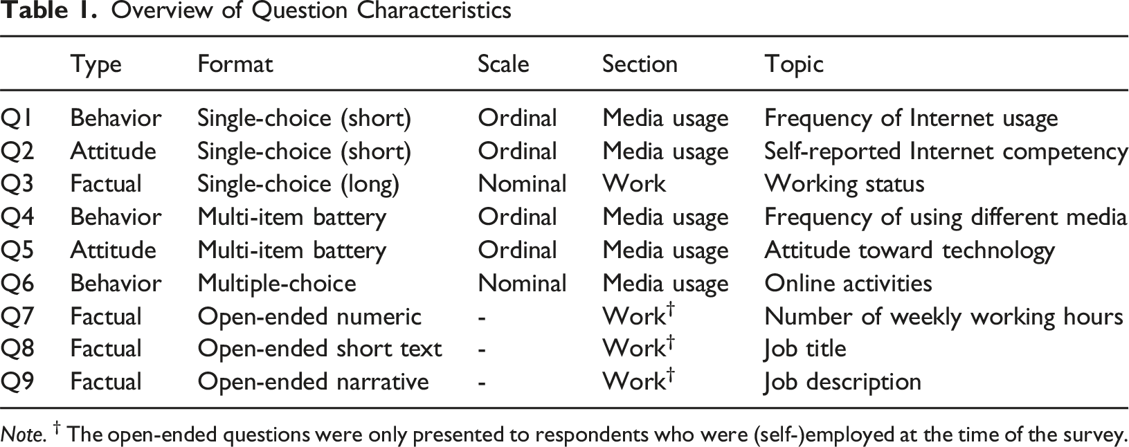
Note. † The open-ended questions were only presented to respondents who were (self-)employed at the time of the survey.
All survey questions were displayed on separate survey pages, although Q4 and Q5 were grid questions containing several items that were presented together on the same survey page. While the wording and formatting of the questions were identical across both surveys (see Table A2 in the Appendix for the full question text and response options), the overall questionnaire length and the other questionnaire sections differed.
Outlier Detection Methods
Overview of Response Time Outlier Detection Methods
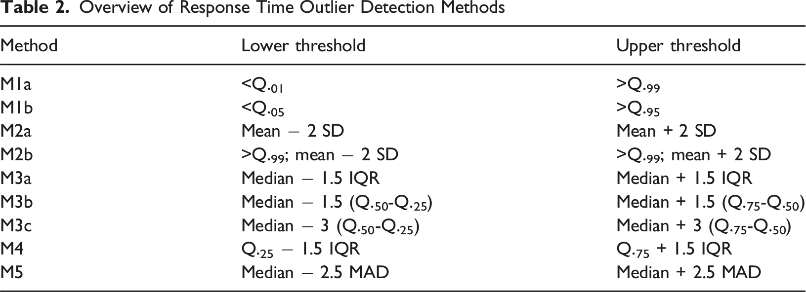
First, we applied two percentile-based cutoffs commonly used in survey research: the top and bottom 1% (M1a) and the top and bottom 5% (M1b). Next, we used two methods based on the mean value and standard deviation. The first, mean ± 2 SD (M2a), is widely regarded as the standard approach in survey research. In the second variant, we first excluded the upper 1% of response times before applying the mean ± 2 SD (M2b), to reduce the influence of extreme long values on the mean.
We also implemented three variations of median-based outlier detection using the interquartile range (IQR). The first uses the median ± 1.5 IQR (M3a). In line with recommendations to calculate separate IQRs above and below the median, we further employed a rather strict threshold of 1.5 times (M3b) and a more moderate threshold of 3 times (M3c) the range between Q.75-Q.50 and Q.50-Q.25, following the procedure used by Höhne and Schlosser (2018). Additionally, we used Tukey’s (1977) method, which defines outliers as falling beyond Q.25 and Q.75, respectively, ± 1.5 IQR (M4).
Finally, we included a method based on the median absolute deviation (MAD), which provides according to Leys et al. (2013) a more robust measure of dispersion than IQR. In this approach, outliers are defined as values falling beyond the median ± 2.5 MAD (M5).
Data Preparation and Analyses
The following criteria had to be met for cases to be included in the analysis; otherwise, they were excluded: (a) respondents were shown the respective survey question (i.e., they did not have a system missing value due to a filter), (b) they provided a valid response to the survey question (i.e., no item nonresponse, including nonsubstantive responses to open-ended questions), (c) they visited the web page containing the survey question only once (i.e., no ‘backtracking’), and (d) the client-side paradata script functioned correctly.
All outlier detection methods were applied separately for each of the nine survey questions and separately for each panel, with the latter ensuring that thresholds were derived from panel-specific response time data, thereby minimizing bias due to differences in sample composition, such as age and device. Regardless of the outlier detection method used, outlier treatment consisted of trimming, that is excluding outliers from analysis, in both panels. No transformation of response time data was performed. The raw response time data is described in Table A3 in the Appendix.
To address RQ1 and the effect of outlier detection methods on response time data, we calculated the share of outliers for each survey question. Chi-square tests of independence were used to assess whether outlier detection methods produced significantly different results across the two panels. To compare the impact of outlier detection methods on mean response time between panels, we conducted MANCOVAs with panel type as the main predictor and gender, age, education, and device type as covariates. All covariates were recoded as binary variables (gender: male vs. female; education: with vs. without a university entrance qualification; device: smartphone vs. desktop), except age, which was treated as a continuous variable.
For RQ2, we examined whether specific respondent groups were systematically more likely to be identified as outliers and whether these patterns varied by panel type. We used the same binary variables for gender, education, and device type, with chi-square tests of independence employed to assess group differences. For age, independent samples t-tests were conducted to test significant differences between outliers and non-outliers.
To visually summarize the findings from the extensive analyses, we created plots using R (version 4.4.2) and the ggplot2 package (version 3.5.2). For each panel and variable, separate plots were generated to display findings across all outlier detection methods and survey questions.
Results
RQ1: How Do Different Outlier Detection Methods Differ in Their Effects on Response Time Data Between Probability and Nonprobability Online Panels?
First, we examined whether the outlier detection methods differed in identifying short and long outliers in the probability versus nonprobability panel (see Figure 1). Detection of Short Outliers, by Method and Question. Dots indicate the detection of short outliers
All methods consistently detected long outliers in both panels (not depicted here). However, clear differences in the detection of short outliers emerged depending on the detection method used, with almost identical patterns observed in both panels. By definition, the percentile-based methods (M1a and M1b) identified short outliers across all questions and in both panels. M3b was the only non-percentile method that consistently identified short outliers across all questions in both panels. In contrast, M2a, M4, and M5 did not identify short outliers for any question in either panel. The IQR-based methods (M3a and M3c) identified short outliers for only one to three questions and did so similarly across panels. M2b identified short outliers for one question only in the probability panel.
Next, we compared the share of outliers detected by each method between the probability and nonprobability panel (see Figure 2; M1a and M1b were not included in the analysis due to fixed percentiles). Differences in Share of Detected Outliers Between Panels, by Method and Question. Blue dots indicate a significantly higher share of outliers in the probability panel; yellow dots indicate a significantly higher share of outliers in the nonprobability panel (p < .05)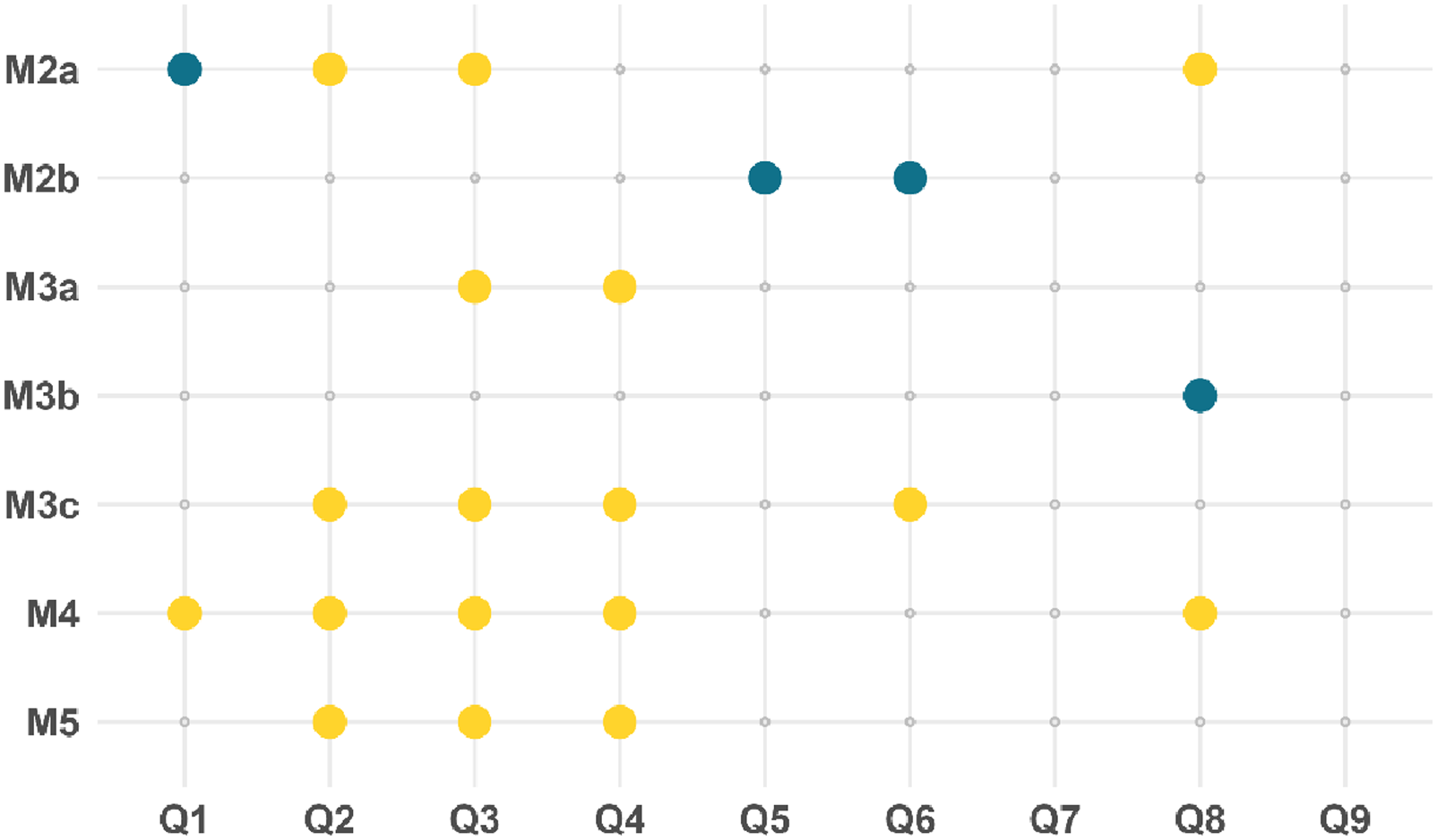
All methods led to significantly different shares of outliers between the probability and nonprobability panel for at least one of the nine questions (21 of 63 differences were significant). Most methods identified a significantly higher share of outliers in the nonprobability panel, suggesting greater irregularity or variation in the response behavior of nonprobability panelists than probability panelists. Only M2b and M3b showed the opposite pattern, identifying significantly more outliers in the probability panel.
Finally, we examined how excluding outliers affected response times. Figure 3 displays the share of outliers, sorted from lowest to highest, averaged across the nine questions (bars) and the ratio of adjusted response time (after outlier exclusion) to the raw response time (before outlier exclusion) averaged across the nine questions (lines). Share of Detected Outliers (%) and Adjusted-to-Raw Response Time Ratio (Basis = 100) Averaged Across the Nine Questions, by Method and Panel Type. * Significant difference at p < .05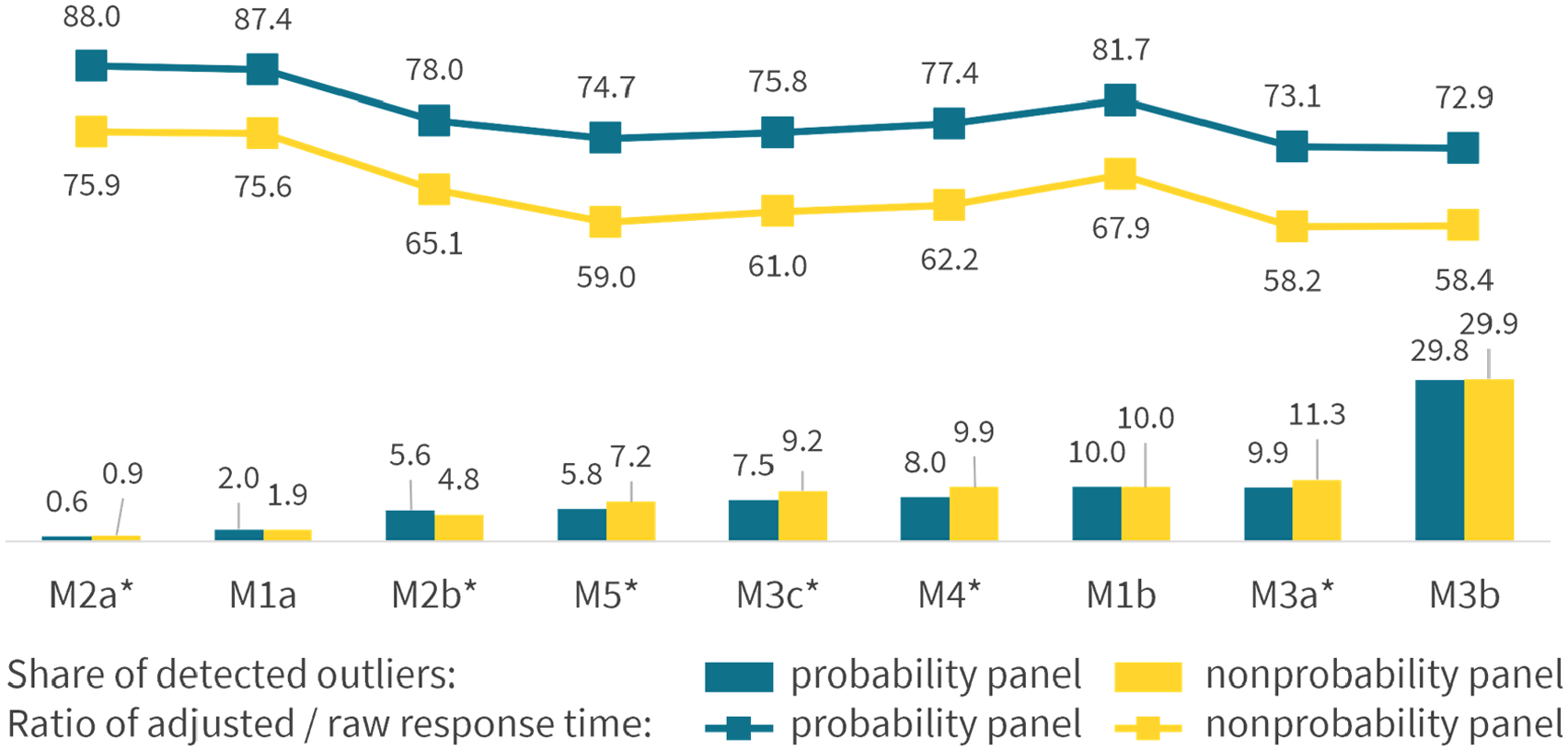
In general, the share of outliers varied considerably depending on the outlier detection method, ranging from 0.6% to 29.9% (see also Table A4 in the Appendix for the share of outliers separately for the nine questions). Although the share of detected outliers differed significantly between panels for nearly all methods (except for and M3b, as well as by definition, for M1a and M1b), these differences were generally small in magnitude (maximum Cramer’s V = 0.03).
Outlier detection methods also differed in how strongly they affected response times. Methods that identified larger shares of outliers tended to produce larger reductions in response times, as reflected in lower adjusted-to-raw response time ratios. Some methods showed non-linear patterns. For instance, M1b removed around 10% of the cases as outliers but produced comparatively smaller reductions in response times; meanwhile, M3b excluded nearly 30% of the cases and yielded reductions in response times similar to those of M3a, which excluded only about 10% of the cases. These patterns were similarly found in both the probability and nonprobability panel and suggest that resulting changes in response times are not strictly linear but depend on the characteristics of the excluded cases. Importantly, the exclusion of outliers had a stronger impact on response times in the nonprobability panel across all methods, leading to overall lower adjusted-to-raw response time ratios in the nonprobability panel compared to the probability panel.
MANCOVAs with the mean adjusted response time (after outlier exclusion) as the dependent variable, panel type as the main predictor, and gender, age, education, and device as covariates (Table A5 in the Appendix) confirmed that response time differences between the panels remained even after controlling for sociodemographic characteristics and therefore could not be attributed to sociodemographic differences.
RQ2: Do Outlier Detection Methods Differ in Terms of Which Respondent Groups Are Identified as Response Time Outliers Between Probability and Nonprobability Online Panels?
To assess whether specific respondent groups were particularly likely to be identified as response time outliers, we compared outliers and non-outliers on gender, age, education, and device type. Figure 4 visualizes significant difference (p < .05) by dots, separately for the probability and nonprobability panel. Dot size reflects the magnitude of the deviation from the overall sample distribution, and color indicates the direction of deviation (i.e., over- vs. underrepresentation). Characteristics of Response Time Outliers by Gender, Age, Education and Device Type. Dots indicate significant differences (p < .05); dot size reflects the magnitude of deviation; color indicates the direction of deviation
Overall, clear differences emerged across methods and panel types, with certain respondent groups being systematically over- or underrepresented among response time outliers. In general, related to age, education, and device type, outliers and non-outliers differed more in the probability panel as indicated by the greater number of significant differences.
Age—and, to a lesser extent, education—showed the most consistent patterns. The percentile-based methods (M1a and M1b) tended to flag younger respondents as outliers, which aligns with the fact that these methods remove a fixed share of the fastest respondents. Especially in the nonprobability panel, where the sample contained a larger proportion of younger respondents, this pattern appeared consistently across all questions. In contrast, most other methods (M2b, M3a, M3c, M4, and M5) more frequently identified older respondents as outliers, suggesting greater sensitivity to slow or variable response behavior. This tendency was more pronounced in the probability panel, which included relatively more older respondents. Thus, part of the observed differences across panels likely reflects differences in their underlying sample compositions (see Table A1 in the Appendix).
A similar but weaker pattern emerged for education. M1a and M1b identified more highly educated respondents as outliers, whereas M2b, M3a, M3c, M4, and M5 tended to classify lower-educated respondents as outliers. This pattern was more obvious in the probability panel, where deviations from the overall sample distribution were more frequent and of larger magnitude, even though the two panels did not differ in education overall.
Patterns for gender and device type were less consistent and more question-specific than those for age and education. For example, Q3 yielded an overrepresentation of men among outliers in the probability panel, while Q9 yielded an overrepresentation of women among outliers in the nonprobability panel. This suggests that certain question types or topics may interact with gender, potentially introducing gender-related biases in response time outliers.
Device-related differences only occurred in the probability panel and for only a few questions. For Q3 and Q4, desktop respondents were mostly overrepresented among outliers, suggesting more variable response behavior among them compared to smartphone respondents. No consistent pattern emerged for the other questions or methods.
Summary and Conclusions
In this study, we examined how different outlier detection methods commonly used in survey research affect response time data in probability and nonprobability online panels, and whether certain respondent groups are systematically more likely to be identified as outliers. By directly comparing two widely used panel types, our study contributes empirical evidence on whether outlier handling procedures function similarly across differently recruited online samples—an issue that has received little attention in previous work.
The main finding is that researchers’ choice of outlier detection method matters, underlining the need for careful method selection in response time analysis. Across all analyses, we observed differences in how outlier detection methods affected the two panel types, though the magnitude and consistency of these differences varied. In both panels, all methods detected long outliers, whereas only a few methods identified short outliers. While the overall share of outliers detected differed substantially by method, the differences between the probability and nonprobability panels were generally small. However, several methods identified significantly higher shares of outliers in the nonprobability panel, suggesting in line with previous assumptions that nonprobability panelists exhibit atypical response behaviors leading to very slow responses more frequently than probability panelists. Different outlier detection methods also varied in how strongly they affected adjusted response times. Outlier exclusion had a stronger impact on response time data in the nonprobability panel than in the probability panel, underscoring higher prevalence or impact of certain response time anomalies in the nonprobability sample.
Moreover, certain respondent groups were systematically over- or underrepresented among response time outliers, and this pattern varied greatly by outlier detection method, highlighting that method choice may influence which respondent groups are disproportionately excluded. Clear differences also emerged between the two panel types. Although age and education effects were present in both panels, the probability panel showed more pronounced group differences between outliers and non-outliers. In general, outlier exclusion may introduce bias if certain subgroups are systematically affected—something that should be considered in analyses of response time data and interpreting the methodological implications for questionnaire design, respondent engagement, and data quality.
Each of the outlier detection methods examined in this paper has distinct advantages and limitations. While percentile-based methods (M1a and M1b) are straightforward to implement by removing a fixed share of cases regardless of the underlying distribution, they produce “arbitrary” consistent results across survey questions and panel types. These methods also risk introducing demographic bias by systematically excluding the fastest respondents who tend to be younger and more highly educated—thus, “falsely flagging [those] who answer particularly quickly due to their cognitive abilities and Internet experience” (Greszki et al., 2015, p. 478). The problem is especially pronounced for short or simple questions, where genuine fast responses are common and percentile trimming may mistakenly classify fast-but-valid responses as outliers.
The mean ±2 SD method (M2a)—although widely used in survey research—is highly sensitive to extremely long response times, which inflate both the mean and SD. Consequently, it consistently fails to detect short outliers and excludes very few cases overall, making it ineffective for trimming response times. This result aligns with Höhne and Schlosser (2018), who found that, aside from the percentile methods, the mean ±2 SD approach is the least effective at identifying discontinuous survey processing, such as when respondents interrupt the survey by switching browser windows or tabs.
Median-based methods are generally less affected by extreme values. However, the strict IQR method (M3b) identifies an unusually high share of outliers (>30%), which leads to an outsized reduction in sample size. Even though this method identifies short outliers without disproportionately flagging certain respondent groups as outliers, its high exclusion rate substantially reduces sample size and raises concerns about its suitability for substantive analysis, especially in studies with small samples. Thus, for very different reasons, M3b, M2a, M1a, and M1b emerge as the least preferred methods for detecting response time outliers.
In contrast, the median-based IQR variations (M3a and M3c) offer the most balanced trade-off in terms of share of cases flagged, sensitivity to both short and long outliers, panel differences, and demographic distortions. In addition, both methods are relatively effective at identifying biased response times due to discontinuous survey processing (Höhne & Schlosser, 2018). Thus, although they identify short outliers only for some questions, they are easy to implement, adapt to differences across panel types, and flag a reasonable share of outliers, enabling a meaningful yet non-disruptive adjustment of response times.
This study has some limitations that provide opportunities for future research. We examined the effects of outlier detection methods using nine methods that are widely applied in survey research. However, variations of these approaches― adaptive percentile cutoffs, question- and device-specific thresholds, or hybrid rules that combine distributional and respondent-level information—may offer more tailored solutions. In addition, entirely different approaches for detecting response time outliers merit attention. Machine learning-based detection techniques or response time modeling that explicitly account for task complexity, cognitive load, and individual speed differences may produce more theoretically grounded definitions of “extreme” response behavior.
Our results are based on the analysis of nine survey questions that vary by type, format, and content. This relatively small number of questions, concentrated in two topical domains, limits the generalizability of our findings to surveys with broader thematic coverage and reduces the ability to disentangle the extent to which observed effects can be attributed to specific design features. For instance, certain question formats (e.g., open-ended questions) appear only within one question type (factual) and a single topical area (work), making it difficult to separate format effects from content or topic effects. Effects may therefore differ for other types of questions and in other substantive domains. Replication studies based on a more extensive set of questions—fully balanced for type, format, and content—would help clarify when and why specific outlier detection methods perform differently and to what extent these differences can be attributed to particular design features. Although we controlled for some sociodemographic variables, future studies might also consider additional factors such as respondents’ topic interest or motivation (Gummer & Roßmann, 2015) to explain variability in response time data. Moreover, although we replicated entire modules from the probability panel in the nonprobability panel, differences in questionnaire length and in other parts of the questionnaire remained, meaning that potential context effects cannot be fully ruled out. Future studies should therefore use fully identical questionnaires when comparing panel types.
Our results comparing panel types are based on a single survey conducted within one probability and one nonprobability panel, which raises questions about the generalizability of our findings. On the one hand, response time data in self-administered online surveys typically exhibit strong right-skewness and extreme values caused by interruptions or multitasking, and these distributional properties are not unique to specific panels. As a result, the relative performance of outlier detection methods—particularly the robustness of median-based approaches compared to mean- or percentile-based methods—is likely to extend to similar online survey contexts. On the other hand, panel-specific characteristics such as recruitment strategies, incentive structures, survey topic, questionnaire length, and other factors affecting cognitive demands may influence response behavior and the prevalence of response time outliers. Future research should therefore replicate these analyses across multiple surveys, panel providers, and panel-specific design features to further assess the scope and limits of this generalizability.
Future research should also examine more closely whether response time outliers—identified through the methods evaluated here—are meaningfully associated with reduced response quality. Prior research suggests that extreme response times can correlate with satisficing behaviors or poorer data quality (e.g., item nonresponse, “don’t know” responses; Greszki et al., 2015; Höhne & Schlosser, 2018). Understanding which outlier detection methods are most predictive of low-quality responses would help clarify when and why trimming is justified. Moreover, the prevalence and implications of response time outliers may depend on study design features such as frequency of data collection, number of waves, and characteristics of the recruited sample (Roßmann & Gummer, 2016). Addressing these aspects would support developing more context-sensitive guidelines for using response time outliers as indicators of data quality and for tailoring outlier detection methods to different types of panel designs and survey populations.
Overall, this study highlights the importance of carefully selecting outlier detection methods when analyzing response time data. Different methods may yield different results depending on question characteristics, panel types, and respondent characteristics. Consequently, researchers should select outlier detection approaches not only for ease of implementation but in alignment with their analytical objectives, the structure of their sample, and the potential for subgroup-specific biases.
Footnotes
Ethical Considerations
The survey data used in the current study were collected in accordance with established ethical standards.
Consent to Participate
In both surveys, respondents were informed that participation was voluntary and could be discontinued at any time. On the welcome page of the survey, participants were informed about the types of paradata collected and that these are used for methodological research only. Contact information in case of questions about the research and research participants’ rights was included on the welcome and closing page of the survey. The survey data was only available to the authors in anonymized form, meaning the datasets did not contain any identifying information. As no sensitive information was included in the datasets, additional approval by the ethics committee for analysis was not required.
Funding
The authors received no financial support for the research, authorship, and/or publication of this article.
Declaration of Conflicting Interests
The authors declared no potential conflicts of interest with respect to the research, authorship, and/or publication of this article.
Data Availability Statement
Appendix
Sample Composition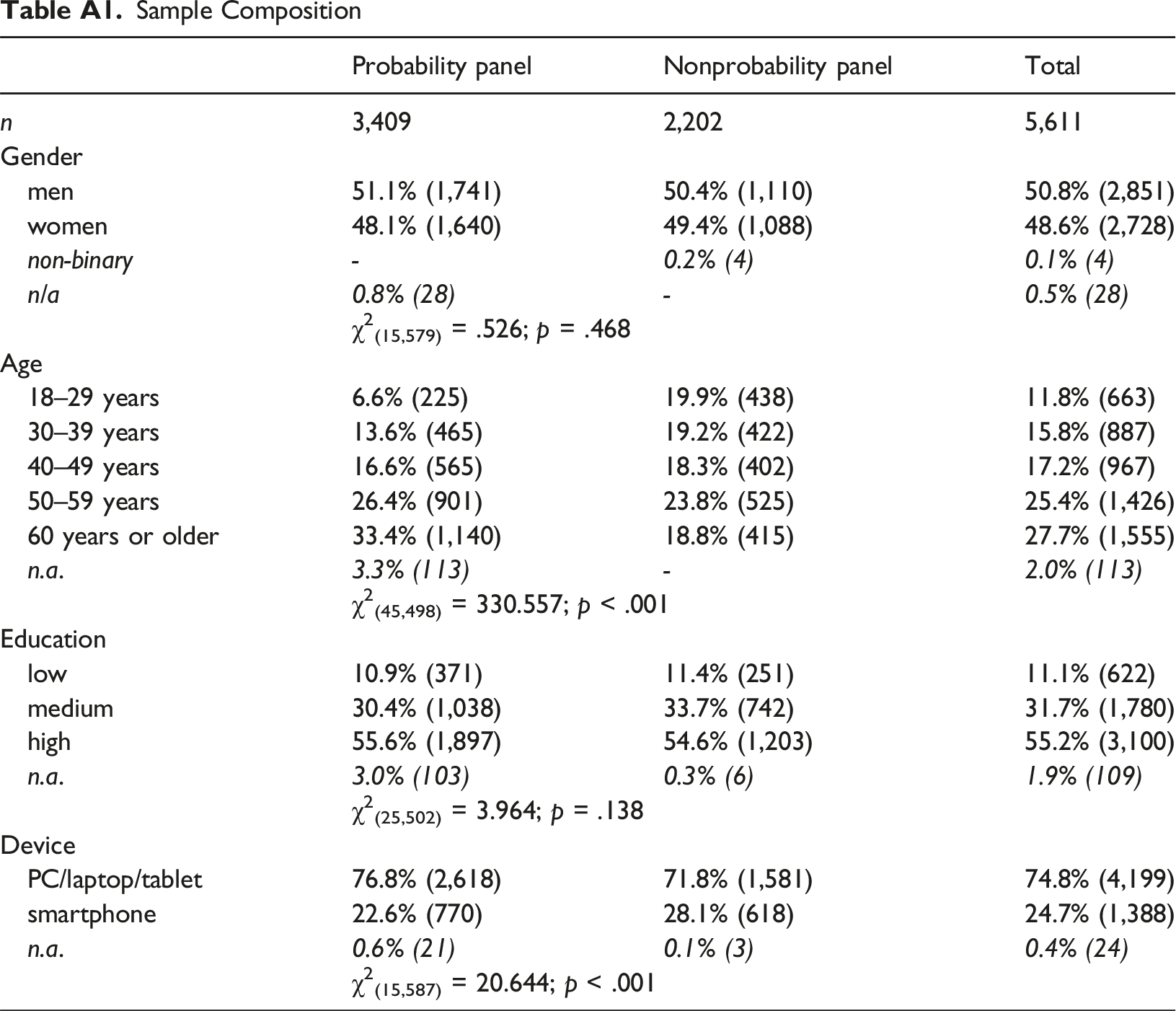
Probability panel
Nonprobability panel
Total
n
3,409
2,202
5,611
Gender
men
51.1% (1,741)
50.4% (1,110)
50.8% (2,851)
women
48.1% (1,640)
49.4% (1,088)
48.6% (2,728)
non-binary
-
0.2% (4)
0.1% (4)
n/a
0.8% (28)
-
0.5% (28)
χ2(15,579) = .526; p = .468
Age
18–29 years
6.6% (225)
19.9% (438)
11.8% (663)
30–39 years
13.6% (465)
19.2% (422)
15.8% (887)
40–49 years
16.6% (565)
18.3% (402)
17.2% (967)
50–59 years
26.4% (901)
23.8% (525)
25.4% (1,426)
60 years or older
33.4% (1,140)
18.8% (415)
27.7% (1,555)
n.a.
3.3% (113)
-
2.0% (113)
χ2(45,498) = 330.557; p < .001
Education
low
10.9% (371)
11.4% (251)
11.1% (622)
medium
30.4% (1,038)
33.7% (742)
31.7% (1,780)
high
55.6% (1,897)
54.6% (1,203)
55.2% (3,100)
n.a.
3.0% (103)
0.3% (6)
1.9% (109)
χ2(25,502) = 3.964; p = .138
Device
PC/laptop/tablet
76.8% (2,618)
71.8% (1,581)
74.8% (4,199)
smartphone
22.6% (770)
28.1% (618)
24.7% (1,388)
n.a.
0.6% (21)
0.1% (3)
0.4% (24)
χ2(15,587) = 20.644; p < .001
Question Wording (English Translation)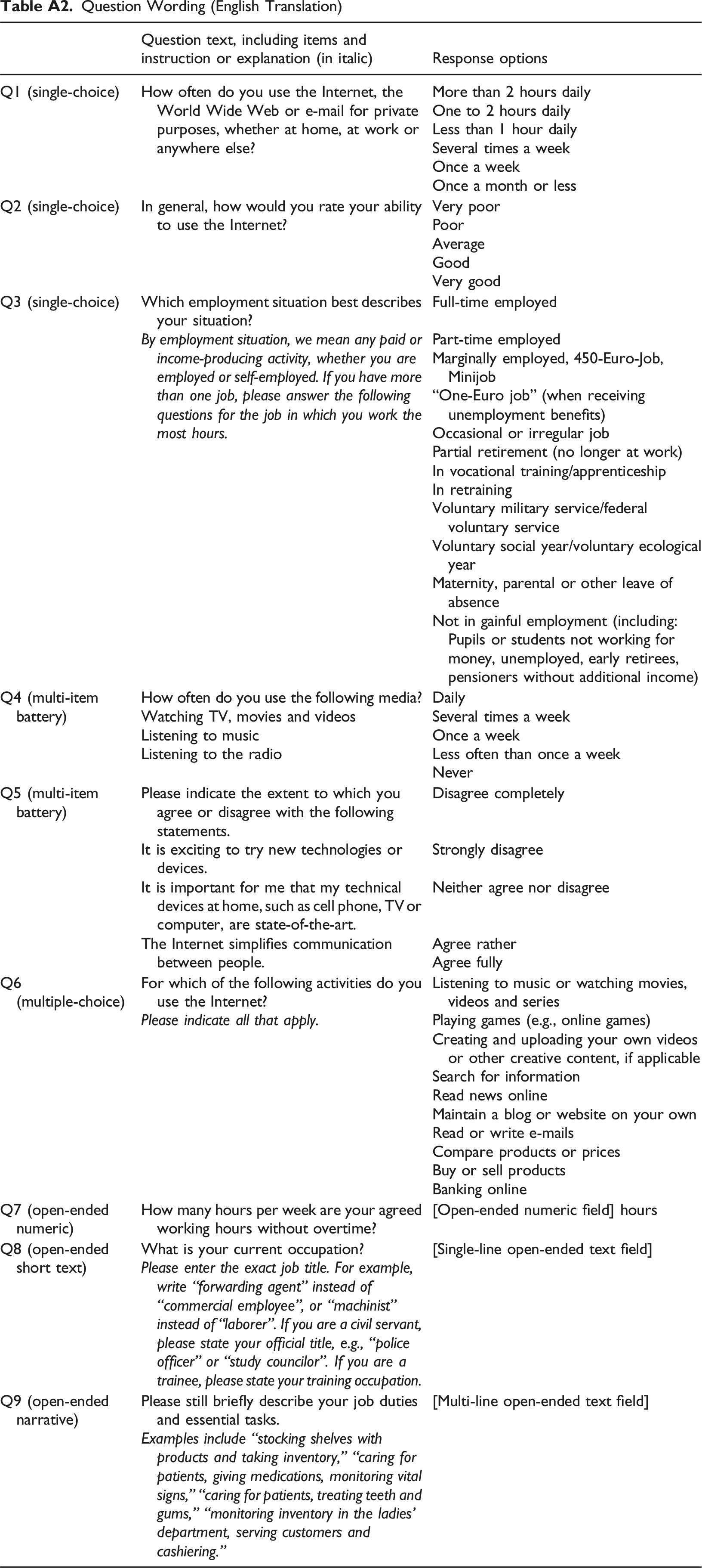
Question text, including items and instruction or explanation (in italic)
Response options
Q1 (single-choice)
How often do you use the Internet, the World Wide Web or e-mail for private purposes, whether at home, at work or anywhere else?
More than 2 hours daily
One to 2 hours daily
Less than 1 hour daily
Several times a week
Once a week
Once a month or less
Q2 (single-choice)
In general, how would you rate your ability to use the Internet?
Very poor
Poor
Average
Good
Very good
Q3 (single-choice)
Which employment situation best describes your situation?
Full-time employed
By employment situation, we mean any paid or income-producing activity, whether you are employed or self-employed. If you have more than one job, please answer the following questions for the job in which you work the most hours.
Part-time employed
Marginally employed, 450-Euro-Job, Minijob
“One-Euro job” (when receiving unemployment benefits)
Occasional or irregular job
Partial retirement (no longer at work)
In vocational training/apprenticeship
In retraining
Voluntary military service/federal voluntary service
Voluntary social year/voluntary ecological year
Maternity, parental or other leave of absence
Not in gainful employment (including: Pupils or students not working for money, unemployed, early retirees, pensioners without additional income)
Q4 (multi-item battery)
How often do you use the following media?
Daily
Watching TV, movies and videos
Several times a week
Listening to music
Once a week
Listening to the radio
Less often than once a week
Never
Q5 (multi-item battery)
Please indicate the extent to which you agree or disagree with the following statements.
Disagree completely
It is exciting to try new technologies or devices.
Strongly disagree
It is important for me that my technical devices at home, such as cell phone, TV or computer, are state-of-the-art.
Neither agree nor disagree
The Internet simplifies communication between people.
Agree rather
Agree fully
Q6 (multiple-choice)
For which of the following activities do you use the Internet?
Listening to music or watching movies, videos and series
Please indicate all that apply.
Playing games (e.g., online games)
Creating and uploading your own videos or other creative content, if applicable
Search for information
Read news online
Maintain a blog or website on your own
Read or write e-mails
Compare products or prices
Buy or sell products
Banking online
Q7 (open-ended numeric)
How many hours per week are your agreed working hours without overtime?
[Open-ended numeric field] hours
Q8 (open-ended short text)
What is your current occupation?
[Single-line open-ended text field]
Please enter the exact job title. For example, write “forwarding agent” instead of “commercial employee”, or “machinist” instead of “laborer”. If you are a civil servant, please state your official title, e.g., “police officer” or “study councilor”. If you are a trainee, please state your training occupation.
Q9 (open-ended narrative)
Please still briefly describe your job duties and essential tasks.
[Multi-line open-ended text field]
Examples include “stocking shelves with products and taking inventory,” “caring for patients, giving medications, monitoring vital signs,” “caring for patients, treating teeth and gums,” “monitoring inventory in the ladies’ department, serving customers and cashiering.”
Descriptives of Raw Response Time Data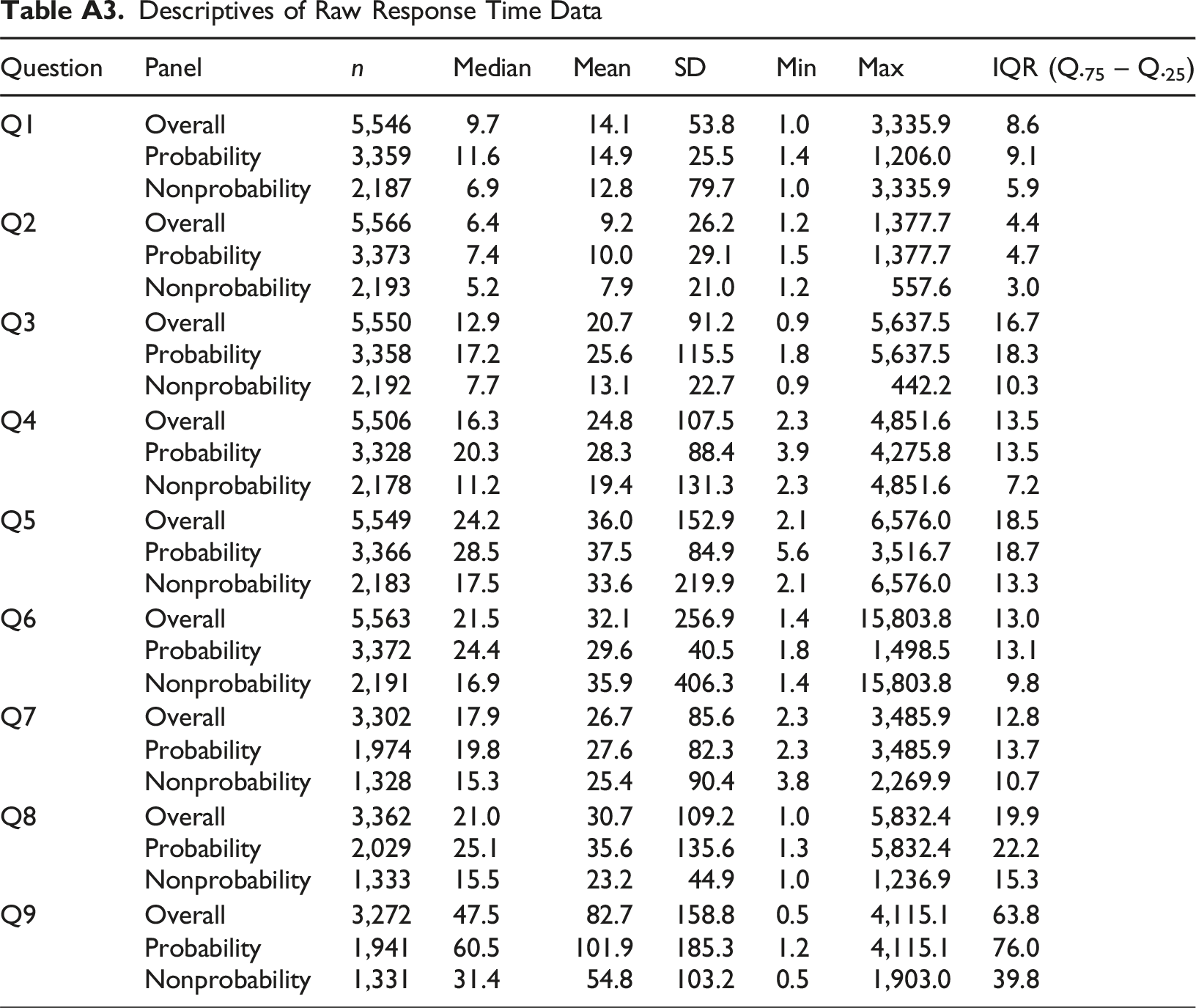
Question
Panel
n
Median
Mean
SD
Min
Max
IQR (Q.75 – Q.25)
Q1
Overall
5,546
9.7
14.1
53.8
1.0
3,335.9
8.6
Probability
3,359
11.6
14.9
25.5
1.4
1,206.0
9.1
Nonprobability
2,187
6.9
12.8
79.7
1.0
3,335.9
5.9
Q2
Overall
5,566
6.4
9.2
26.2
1.2
1,377.7
4.4
Probability
3,373
7.4
10.0
29.1
1.5
1,377.7
4.7
Nonprobability
2,193
5.2
7.9
21.0
1.2
557.6
3.0
Q3
Overall
5,550
12.9
20.7
91.2
0.9
5,637.5
16.7
Probability
3,358
17.2
25.6
115.5
1.8
5,637.5
18.3
Nonprobability
2,192
7.7
13.1
22.7
0.9
442.2
10.3
Q4
Overall
5,506
16.3
24.8
107.5
2.3
4,851.6
13.5
Probability
3,328
20.3
28.3
88.4
3.9
4,275.8
13.5
Nonprobability
2,178
11.2
19.4
131.3
2.3
4,851.6
7.2
Q5
Overall
5,549
24.2
36.0
152.9
2.1
6,576.0
18.5
Probability
3,366
28.5
37.5
84.9
5.6
3,516.7
18.7
Nonprobability
2,183
17.5
33.6
219.9
2.1
6,576.0
13.3
Q6
Overall
5,563
21.5
32.1
256.9
1.4
15,803.8
13.0
Probability
3,372
24.4
29.6
40.5
1.8
1,498.5
13.1
Nonprobability
2,191
16.9
35.9
406.3
1.4
15,803.8
9.8
Q7
Overall
3,302
17.9
26.7
85.6
2.3
3,485.9
12.8
Probability
1,974
19.8
27.6
82.3
2.3
3,485.9
13.7
Nonprobability
1,328
15.3
25.4
90.4
3.8
2,269.9
10.7
Q8
Overall
3,362
21.0
30.7
109.2
1.0
5,832.4
19.9
Probability
2,029
25.1
35.6
135.6
1.3
5,832.4
22.2
Nonprobability
1,333
15.5
23.2
44.9
1.0
1,236.9
15.3
Q9
Overall
3,272
47.5
82.7
158.8
0.5
4,115.1
63.8
Probability
1,941
60.5
101.9
185.3
1.2
4,115.1
76.0
Nonprobability
1,331
31.4
54.8
103.2
0.5
1,903.0
39.8
Share of Outliers, by Outlier Detection Method, Question, and Panel Type Note. * Significant differences at p < .05.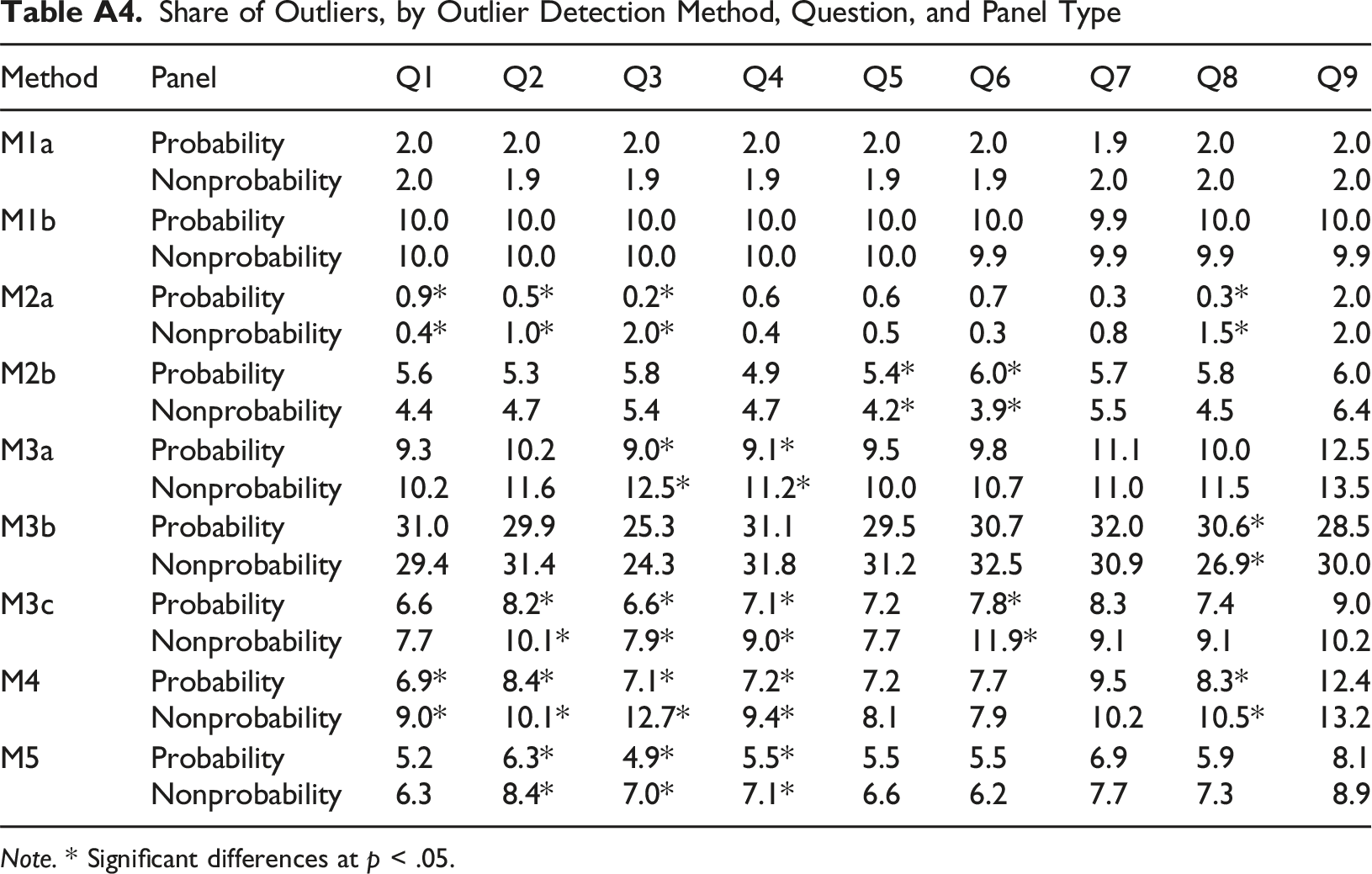
Method
Panel
Q1
Q2
Q3
Q4
Q5
Q6
Q7
Q8
Q9
M1a
Probability
2.0
2.0
2.0
2.0
2.0
2.0
1.9
2.0
2.0
Nonprobability
2.0
1.9
1.9
1.9
1.9
1.9
2.0
2.0
2.0
M1b
Probability
10.0
10.0
10.0
10.0
10.0
10.0
9.9
10.0
10.0
Nonprobability
10.0
10.0
10.0
10.0
10.0
9.9
9.9
9.9
9.9
M2a
Probability
0.9*
0.5*
0.2*
0.6
0.6
0.7
0.3
0.3*
2.0
Nonprobability
0.4*
1.0*
2.0*
0.4
0.5
0.3
0.8
1.5*
2.0
M2b
Probability
5.6
5.3
5.8
4.9
5.4*
6.0*
5.7
5.8
6.0
Nonprobability
4.4
4.7
5.4
4.7
4.2*
3.9*
5.5
4.5
6.4
M3a
Probability
9.3
10.2
9.0*
9.1*
9.5
9.8
11.1
10.0
12.5
Nonprobability
10.2
11.6
12.5*
11.2*
10.0
10.7
11.0
11.5
13.5
M3b
Probability
31.0
29.9
25.3
31.1
29.5
30.7
32.0
30.6*
28.5
Nonprobability
29.4
31.4
24.3
31.8
31.2
32.5
30.9
26.9*
30.0
M3c
Probability
6.6
8.2*
6.6*
7.1*
7.2
7.8*
8.3
7.4
9.0
Nonprobability
7.7
10.1*
7.9*
9.0*
7.7
11.9*
9.1
9.1
10.2
M4
Probability
6.9*
8.4*
7.1*
7.2*
7.2
7.7
9.5
8.3*
12.4
Nonprobability
9.0*
10.1*
12.7*
9.4*
8.1
7.9
10.2
10.5*
13.2
M5
Probability
5.2
6.3*
4.9*
5.5*
5.5
5.5
6.9
5.9
8.1
Nonprobability
6.3
8.4*
7.0*
7.1*
6.6
6.2
7.7
7.3
8.9
MANCOVAs on Mean Adjusted Response Times, by Outlier Detection Method Note. *p < .05; **p < .01; ***p < .001. dfh = hypothesis degrees of freedom, dfe = error degrees of freedom.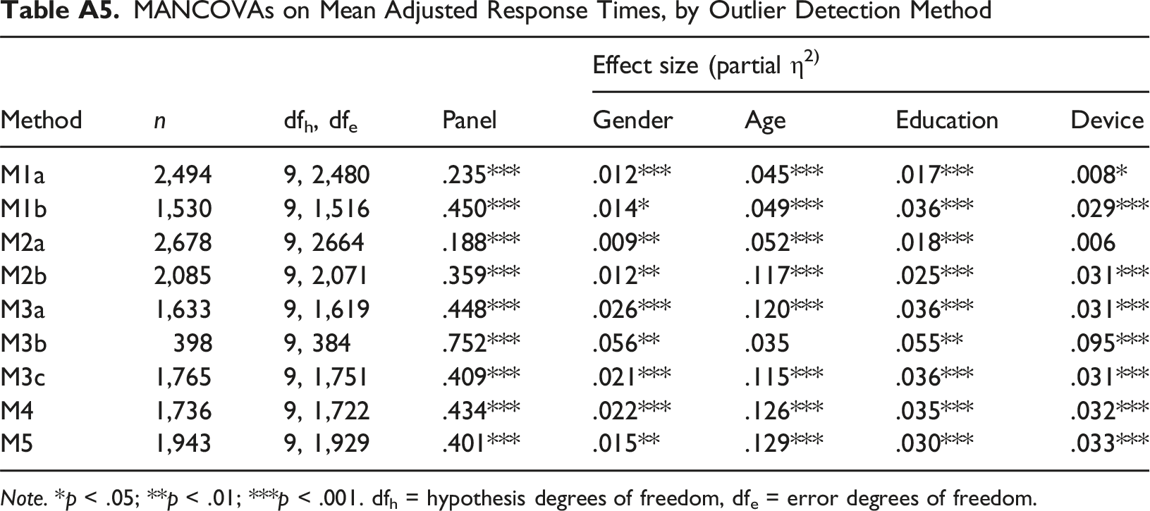
Method
n
dfh, dfe
Effect size (partial η2)
Panel
Gender
Age
Education
Device
M1a
2,494
9, 2,480
.235***
.012***
.045***
.017***
.008*
M1b
1,530
9, 1,516
.450***
.014*
.049***
.036***
.029***
M2a
2,678
9, 2664
.188***
.009**
.052***
.018***
.006
M2b
2,085
9, 2,071
.359***
.012**
.117***
.025***
.031***
M3a
1,633
9, 1,619
.448***
.026***
.120***
.036***
.031***
M3b
398
9, 384
.752***
.056**
.035
.055**
.095***
M3c
1,765
9, 1,751
.409***
.021***
.115***
.036***
.031***
M4
1,736
9, 1,722
.434***
.022***
.126***
.035***
.032***
M5
1,943
9, 1,929
.401***
.015**
.129***
.030***
.033***