
Abstract
Machine learning classifiers are increasingly widely used. This research note explores how a particular widely used classifier, the Random Forest, performs when faced with samples which are imbalanced and noisy data. Both are known to affect accuracy, but if their effects are independent or not has not been explored. Based on an experiment using synthetic data generated for the study we find that the effects of noise and sample balance interact with each other; classification accuracy is worse when faced with both noisy data and sample imbalance. This has implications for the use of RF in market research, but also for how methods to address either sample imbalance or noise are assessed.
Introduction
Machine learning algorithms are increasingly attracting attention from management and marketing researchers (e.g., Choudhury et al., 2021) and studies employing them are increasingly appearing in IJMR (e.g., Ekinci & Güran, 2022; Rausch et al., 2022). Valizade et al. (2022) argue that a machine learning approach can complement, and in some circumstances supplant, the dominant (hypothesis-testing) approach to quantitative research. However, in using such algorithms researchers have to accept a trade-off between the learning capacity of the algorithm and how interpretable its output is (e.g., Weller et al., 2021). There is also an increasing awareness of the limitations of these methods, particularly when they are faced with unbalanced samples and noisy data. This note focuses on how well the widely used Random Forest (RF) algorithm performs with such data. First, we illustrate how RF classification accuracy is affected by noise and by sample imbalance. Second, we show how the effects of these two influences combine to affect classification accuracy; accuracy worsens when faced with both unbalanced data and higher levels of noise by more than the sum of the combined direct effects.
Random Forests are a type of classifier first proposed by Breiman (2001) based on decision trees combined with aggregation and bootstrap ideas. The algorithm arguably offers both learning capacity and interpretability (e.g., Hain & Jurowetzki, 2020). Compared to other ensemble Machine Learning methods, Random Forests are described as easier to interpret as they can identify influential predictors. They also tend to be at least as accurate as both other ensemble Machine Learning classifiers and classical classifiers such as logistic regression. These characteristics have led Random Forests to be described as the best “off-the-shelf” algorithm (e.g., Conn & Ramirez, 2016), hence our focus on them. Random Forests rival other methods across a range of areas. For example, Aggarwal and Zhai (2012) propose Random Forests (RF), Support Vector Machines (SVM) and Naïve Bayes (NB) as the most effective classifiers in text mining. In Kobayashi et al. (2018) test of classifier performance in text mining, RF, SVM and NB all performed well with accuracy above 95%. However, both RF and SVM significantly outperformed NB. Random Forests have also been found to perform well in sales forecasting. Loureiro et al. (2018) found that random forests performed as well as deep learning networks in fashion retail forecasting. Similarly, Rausch et al. (2022) found the random forest algorithm to be one of the better performing classification methods out of the 13 they apply to shopping cart abandonment.
Given their performance and the comparative ease with which they can be implemented, it becomes more important for researchers to know what can affect RF classification accuracy. Two influences on classifier accuracy have been identified in the literature: class imbalance, i.e., one of the categories in the target variable being much less prevalent than others; and the amount of noise in the data. These have however tended to be investigated separately. For example, research on decision trees, the building blocks of RF by Coussement et al., 2014, suggests that increasing noise in the data would adversely affect their predictive accuracy. Similarly, increasing class imbalance would have negative impact on RF performance (Brown & Mues, 2012).
The aim of this study is to determine whether these influences operate independently or if the incidence of one affects the severity of the other and so to inform best practice recommendations for use of RF as a robust machine learning classifier.
Challenges to classification accuracy: Class imbalance and noise
Classifiers have difficulty in differentiating between classes in the target variable in samples where there are many more observations in one class than the other. They can still achieve high overall accuracy by classifying many or even all observations as belonging to the majority (most frequently occurring) class. For example, say we have a target variable with the outcome of interest occurring 10 times out of 100 giving a variable with 10 1 s and 90 0 s. A classifier can achieve 90% overall accuracy by predicting all 100 observations to have a value of 0. An overall accuracy of 90% looks good but conceals an error rate for classifying 1 s of 100%. Arguably it is the rarer outcomes which are the more interesting.
A number of approaches to correcting for sample imbalance have been suggested. These include adjusting the available data through random under-sampling (dropping cases from the majority class selected at random) and random over-sampling (adding cases to the minority class). Others include the Synthetic Minority Oversampling Technique (SMOTE) (Chawla et al., 2002) and the Adaptive Synthetic or ADASYN method (He et al., 2008). Several studies have explored the performance of these methods but, as Leevy et al. (2018) note, the results are not entirely consistent.
The second challenge to classification accuracy is noise in the data. This is potentially the more troublesome as it is more difficult to detect. Two sources of noise have been investigated: class noise and attribute noise (e.g., Khoshgoftaar et al., 2005). Class noise refers to noise in the dependent or target variable and could arise from misclassification or other data entry/data capture errors. Attribute noise refers to noise in the explanatory variables. Such noise can arise from data coding or data capture errors. The robustness of Random Forests when faced with label noise has also attracted attention. Ghosh et al. (2017) identify that Random Forests are robust to label (or class) noise if the noise is symmetric (where all classes of the target variable are equally noisy) and the sample is large enough. However, where noise is asymmetric the classifier is not robust.
Noisy features are more likely to arise in Management and Social Science applications of the classifier than elsewhere. Noise and uncertainty will be inherent in data which captures the results of human decisions. Such noise can arise from measurement issues, especially where focal variables are not directly observable (for example in inferred data or attitudinal data). However, it can also arise from variations in the explanatory power a variable has across cases in the sample. In such applications rather arising from errors in the data, the noise masks the signals the classifier is trying to detect; in such data imprecision is unavoidable.
Aim of the study
The aim of this study is to explore whether the effects of sample imbalance and of noise (in the attribute and class variables) operate independently or whether they interact with each other. Studies suggesting ways of addressing sample imbalance (e.g., Chen et al., 2004) and noise (e.g., Bonissone et al., 2010; Reis et al., 2019) have tended to look at them in isolation. The aim of this study is to identify if these two influences on classification accuracy are independent of each other. If sample imbalance and noise effects reinforce each other, it has implications for evaluating the performance of both random forest classifiers and approaches to address sample imbalance and noise.
Methods and data
Our study adopts a 2 by 2 factorial experiment design. The two factors in the experiment are class imbalance (with two levels: balanced and imbalanced) and noise (also with two levels: low noise and high noise). Synthetic data sets were created in preference to adding noise to a pre-existing data set as both the underlying data generating process and the degree of noise are known.
We employ two generated datasets; one with low noise and one with high noise. As an initial step, randomly generated data were fed into a logistic equation (equation (1))


A total of 2,000 observations were generated for the low noise and high noise conditions. The balanced and imbalanced samples were drawn from these pools of data, each sample containing 400 observations. To create balanced samples, 200 observations where y = 1 and 200 where y = zero were selected at random. For the imbalanced samples, 280 observations where y = zero and 120 where y = 1 were drawn, giving a 70:30 split. Subsamples were drawn from the data set to reduce the time it took to run the analysis. Random Forest calculations are demanding in terms of computing time. For example, in Rausch et al.’s (2022) study, the Random Forest took 171,587 seconds (or just under 48 hours) to complete (the fastest methods: logistic regression, decision tree and boosted logistic regression took 20.3, 225.07 and 380.0 seconds respectively). Ten samples were drawn for each condition giving 40 samples in total: 10 low noise, balanced; 10 high noise, balanced; 10 low noise, imbalanced and 10 high noise, imbalanced.
The random forests were run in R (R Core Team, 2021) using the randomForest package (Liaw & Wiener, 2002). Whilst this allows for different parameters to be tuned (such as the number of trees and number of variables selected as candidates at each split), the defaults were retained for all runs to ensure comparability across all conditions of the experiment. Each run used 500 trees and the number of variables considered at each node of the tree was the square root of the number of the total number of variables.
Five standard measures of classification accuracy are considered: out of bag (OOB) error rate, class zero error, class 1 error, precision and recall. Out of bag error rate (also called the hit rate) is an overall measure of accuracy, averaging across the proportion of 1 s misclassified as 0 s and of 0 s misclassified as 1 s. Although OOB is reported below, it is not included in our analysis, because of the limitations of overall accuracy measures. The class 0 and class 1 error rates are the proportion of 0 s and 1 s which are misclassified. In imbalanced samples, the error rate of the more prevalent class is likely to be lower. For example, with 70% 0 s and 30% 1 s in a sample, classifying everything as zero would give a 30% class 0 error rate, whereas in balanced sample (with a 50:50 split), classifying everything as zero would give a zero class error rate of 50%. For practical applications, the class 0 error rate is arguably less useful than class 1 error rate as we are usually more interested in predicting that an outcome occurred rather than it did not occur. We also report two measures of accuracy of classifying positive outcomes, known as precision and recall. Precision is calculated as the proportion of true positives (1 s classified as 1 s) divided by the sum of true positives and false positives (0 s classified as 1 s). Precision can also be calculated from the Class 1 error rate: Precision = 1 - Class 1 error rate. Recall is calculated as the proportion of true positives divided by the sum of true positives and false negatives (1 s classified as 0 s). These latter two measures have a more intuitive interpretation: the higher the value, the greater the accuracy of the classifier.
Results
Classification accuracy measures averaged over 10 runs per condition.
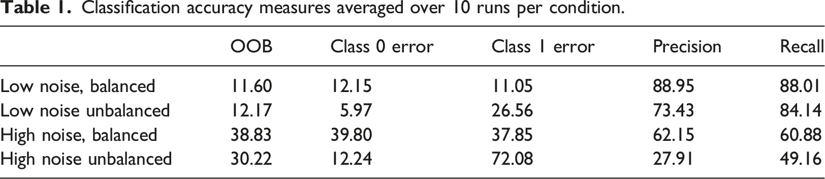
Table 1 shows that, as would be expected, the Random Forest performs well in the low noise and balanced sample condition. The OOB error rate increases slightly in the low noise unbalanced condition compared to the low noise balanced condition, but both are much lower than in the high noise conditions. However, looking at the class zero and class 1 error rates reveals an important difference between the balanced and unbalanced conditions. Class 0 error rates are lower in the unbalanced conditions than the balanced conditions. In the balanced conditions the class 0 and class 1 error rates are similar. In the unbalanced conditions however, the random forest is able to classify 0 s correctly (as there are more of them) but it has more difficulty classifying 1 s (which are rarer). The Class 1 error rate increases to 37.85% in the high noise balance condition but is almost double that at 72.08% in the high noise unbalanced condition. In other words, it classifies almost three quarters of the 1 s in the target variable incorrectly. Our unbalanced samples are not highly unbalanced (at a 70%:30% split or 2.33 to 1) compared say to Leevy et al.’s (2018) definition of high imbalance as a majority to minority ratio of between 100 to 1 and 10,000 to 1, yet we see a decline in classification accuracy compared to the balanced samples. Another way of looking at it is to say the class 1 error rate of the low noise unbalanced samples (26.56%) is more than double that of the low noise balanced samples (11.05%). In the high noise conditions the difference is even greater – the unbalanced sample error rate is almost three times as high as in the balanced samples. This would seem to suggest that the two effects reinforce each other.
Two-way ANOVA results.
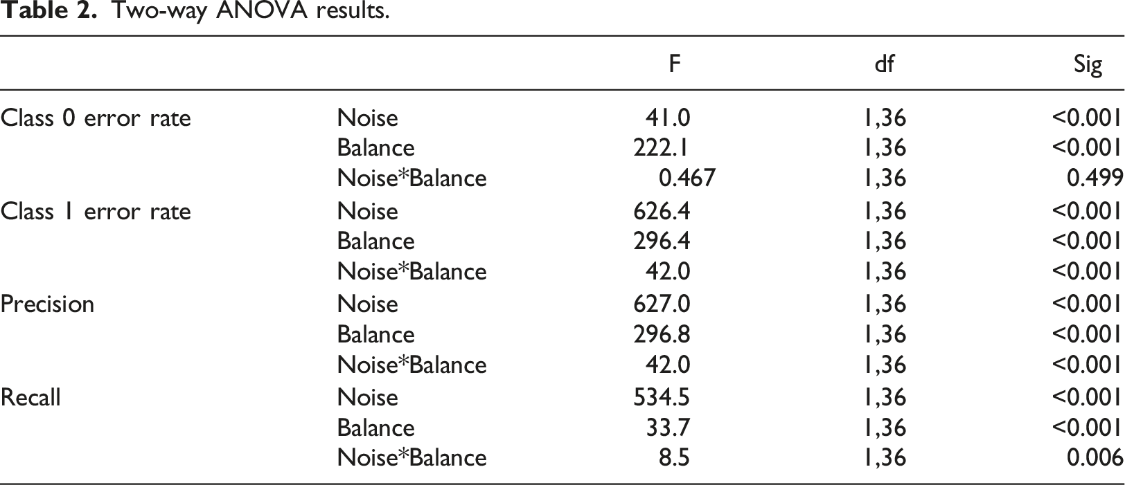
For the class 0 error rate, noise and sample imbalance show significant direct effects, but the interaction between them is not significant. Both noise and imbalance affect the classifier’s ability to correctly identify negative outcomes (i.e., 0 s). The results for class 1 error rate confirm what the results in Table 1 suggest. Both noise and sample imbalance significantly increase the class 1 error rate, but they do not do so independently. The interaction term is also significant suggesting that the effect on class 1 error rate is greater than the sum of the direct effects (similar results are seen for Precision as expected it is related by definition to class 1 error). Recall shows a similar pattern of results with significant direct effects and a significant interaction effect. Thus, it seems that the effects of these two influences on classifier accuracy do not operate independently.
Discussion
Machine learning methods, such as RF, are able to unlock insights from data which might not be achievable using traditional statistical methods, especially with the volume of data which is now available. They underpin for example recommendation systems and personalisation systems and work ‘behind the scenes’ in automated text/sentiment analysis. However, for all their abilities the results here demonstrate that, similar to human decision-makers being prone to inherent cognitive biases, RFs can be biased by the nature of the data they are presented with. Unfortunately, it seems that situations Market Researchers typically face, such as trying to identify the drivers of comparatively rare events and dealing with noisy data, are those which pose a challenge to the random forest algorithm. Moreover, the effects of sample imbalance and noise reinforce each other.
It is often the rarer cases which are of most interest, for example customers who will be high-value in the future, or customers who are likely to switch brands. Unfortunately, the results show that even a moderate imbalance between classes can have a significant impact on RF classification performance. The impact appears to be most significant for Class 1 errors. This is perhaps not surprising as it is the least represented class but is also worrying as it tends to be the class we are interested in. The impact of noise in the data on random forest classification accuracy is also significant. Moreover, the combined effects of noise and imbalance are significant for Class 1 classification performance (and recall and precision) but not for class 0. In other words, classification accuracy worsens when the algorithm is faced with data which is both noisy and unbalanced, compared to when dealing with data which is either noisy or unbalanced.
Of the two influences on accuracy, sample imbalance can be more readily observed making it easier to take actions to reduce its effects. Unfortunately, the same cannot be said for noise. Fortunately, the results suggest that addressing sample imbalance will improve classifier accuracy in high noise conditions. The results also suggest that the potential impact of noise should be considered when comparing classifier performance across different datasets – and in particular when comparing the performance of measures to mitigate the effects of sample imbalance.
The results suggest that both sample imbalance and noise mitigation methods should be used as checks for the robustness of random forest findings. Sample imbalance methods are arguably the easier to implement. Perhaps the simplest approaches involve under-sampling or over-sampling the data. The algorithm would be run twice: once on the full data set and once where the two classes are balanced and the results compared. Alternatively, methods such as SMOTE, ADASYN or cost-sensitive classifiers where there is a bigger penalty for misclassifying the rarest class in the data could be used (Das et al., 2018, provide a useful overview of possible approaches to sample imbalance). It is very encouraging to see methods for accommodating sample imbalance being employed in recent applications of RF in Market Research, for example in Ekinci and Güran’s (2022) study. This we argue should become routine practice. Similarly, researchers should consider comparing performance across different classifiers (e.g. Williams et al., 2023) to benchmark their findings.
Footnotes
Declaration of conflicting interests
The author(s) declared no potential conflicts of interest with respect to the research, authorship, and/or publication of this article.
Funding
The author(s) received no financial support for the research, authorship, and/or publication of this article.