
Abstract
Pendulum systems coupled with springs exhibit nonlinear and coupled dynamics that are difficult to model with purely analytical or numerical approaches. This study investigates a dual-spring pendulum using a hybrid framework that integrates Lagrangian mechanics, Runge–Kutta numerical integration, and physics-informed neural networks (PINNs). The equations of motion are derived via the Lagrangian method, and high-fidelity RK45 solutions are used to pre-train a deep neural network, which is subsequently refined through a physics-based loss function. Comparative simulations under multiple initial conditions demonstrate that the PINN surrogate model preserves phase space structure, achieves high accuracy, and shows strong generalization with errors on the order of 10−3. The findings highlight the effectiveness of combining deep learning with classical mechanics for modeling complex oscillatory systems, offering a pathway toward real-time prediction and control of nonlinear mechanical devices.
Introduction
Considered as models for understanding periodic motion, energy exchange, and the nature of conservative systems, pendulum systems have been fundamental in the evolution of classical mechanics. From Galileo’s early experiments to contemporary applications, the pendulum has fascinated researchers and teachers alike due to its analytical depth and broad applicability.1–3 Fundamentally, the pendulum consists of a mass hung under the effect of gravity from a light, inextensible cord. Especially at higher amplitudes when the restoring torque deviates from the linear approximation,4,5 this basic system provides great understanding of harmonic motion and nonlinear behavior.
When further pressures or limitations are applied, though, the physical pendulum develops into more intricate shapes. Variants include the torsional pendulum, spring-mass pendulum, and Wilberforce pendulum, which combine elements such as elasticity, rotational inertia, and coupling processes, thereby demanding sophisticated mathematical methods for study.6,7 In engineering, seismology, robotics, and biophysics—where dynamic models are often driven by nonlinear differential equations defying closed-form solutions—these systems find extensive use.
One such difficult arrangement results from coupling a pendulum to horizontal springs. Under this method, the pivot point of the pendulum is not fixed but rather attached to a large body limited by symmetrically placed linear springs. This setup introduces a dual source of restoring forces: gravitational torque and spring-induced tension. The resulting dynamics become inherently nonlinear and coupled, particularly when both the angular displacements and translational shifts of the base mass interact with each other. Analytical techniques, such as Lagrangian mechanics, offer a structured approach for deriving the equations of motion (EOMs) and understanding energy transfer within multi-degree-of-freedom systems. 8
Despite the elegance of classical mechanics, analytical methods often fall short when solving highly nonlinear or chaotic regimes, particularly in the presence of damping, forcing, or strong coupling effects. To overcome these challenges, researchers have turned to numerical and computational techniques. While conventional solvers like Runge–Kutta offer reliable time-domain solutions, they are limited in generalization and can suffer from numerical instabilities when simulating long-term behaviors or stiff systems9,10
In recent years, machine learning and neural network-based approaches have emerged as powerful alternatives for modeling dynamical systems. In particular, hybrid neural surrogate models, which combine data-driven learning with physics-informed regularization, offer enhanced stability, interpretability, and predictive power.11,12 These models are particularly effective in capturing both local and global dynamics without requiring manual tuning of equations or incurring excessive computational costs.
Linka et al. 13 applied machine learning to dynamical systems by combining neural networks with Bayesian inference and physics-informed modeling, creating a hybrid framework that enhances generalizability, accuracy, and robustness even with sparse data. Combining physics-informed machine learning (PIML) with recurrent neural architectures, such as neural oscillators, is a viable option for improving its generalization. As established by Kapoor et al., 14 this approach effectively captures long-term dependencies in PDE-governed systems, resulting in improved performance in extrapolation problems that extend beyond the domain of the training data.
Shannon et al. 15 proposed a physics-informed hybrid reservoir computing strategy to address the problem of surrogate modeling for nonlinear oscillator networks. Their approach, which combines an expert analytical model with a reservoir computer, exhibits greater fidelity and improved accuracy for short-term predictions, regardless of whether the expert model contains errors or is incomplete.
Qayyum and Abeer 16 investigated the use of physics-informed neural networks (PINNs) for solving the Kuramoto system of coupled differential equations. Their findings indicate that PINNs can efficiently solve these complex equations while also assessing the system’s synchronization capabilities. The experimental results demonstrate that PINNs are an effective tool for solving differential equations and analyzing the behavior of dynamical systems.
Chen et al. 17 presented a unique numerical technique for analyzing a fractal nonlinear oscillator that simulates a MEMS device by integrating a fractal complex transformation with the spreading residue harmonic balance method. Their method produced highly precise approximations for the system’s vibrations and frequencies, exceeding existing techniques such as the Runge–Kutta method in comparative analysis. The study also includes a sensitivity analysis to better understand the numerical behavior under different settings.
In this study, we propose a physics-informed neural network (PINN) framework to investigate the dynamics of a dual-spring pendulum system. The novelty of this work lies in integrating Lagrangian mechanics, numerical integration (RK45), and a PINN scheme. This combined strategy enables accurate simulation, preserves phase space, and facilitates efficient learning of complex mechanical behaviors under various initial conditions. The presented approach is not only computationally effective but also opens avenues for real-time modeling and control of coupled nonlinear oscillatory systems.
The model under investigation
The physical configuration under investigation is a pendulum of length (ℓ) with a lightweight bob of mass The model.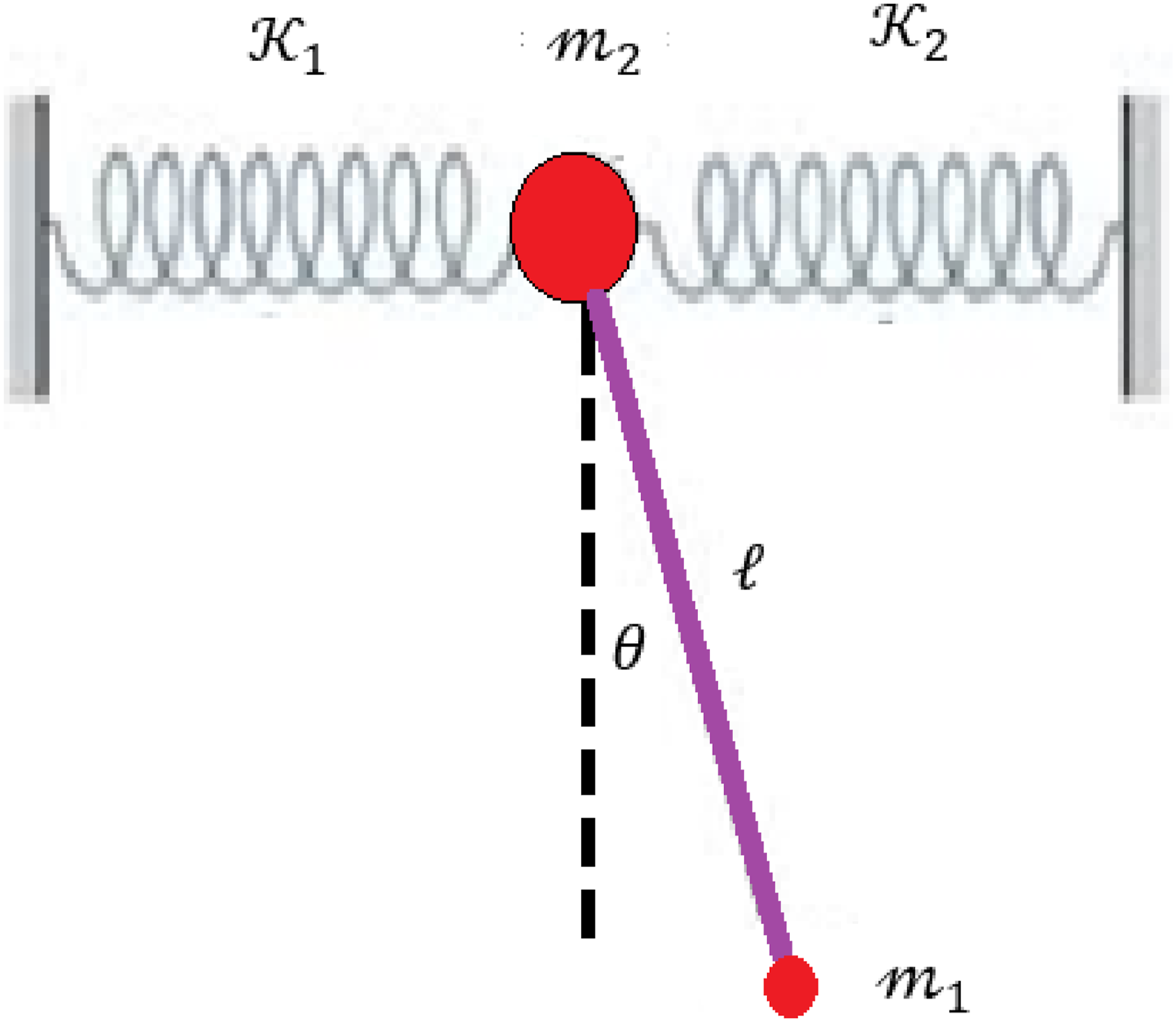
This model aims to infer the equations of motion governing the system while taking into account the elastic forces from the springs, the tension in the string, and the gravitational pull on the pendulum. This configuration offers a rich environment for examining the system’s dynamic behavior, particularly how the combined motion and resistance provided by the two springs influences the pendulum’s oscillations.
Here we aim to derive the Euler-Lagrange equations of motion (ELEs), commonly just referred to as the equations of motion (EOMs.). Primarily, these equations describe how a physical system evolves over time. Defining the classical Lagrangian

The kinetic energy

While the potential energy (

Substituting (2) and (3) into (1) yields:


Derivation of ELEs
Including equation (4) into the fundamental Lagrangian formula


Physics-informed neural network modeling of coupled nonlinear ODEs
In this paper, a physics-informed neural network (PINN) technique is used to model the dynamics of the system governed by second-order nonlinear ordinary differential equations (ODEs) which define the coupled evolution of coordinates
It is difficult to model nonlinear mechanical systems using second-order ordinary differential equations (ODEs) due to their stiffness, oscillatory nature, and sensitivity to initial conditions. Runge–Kutta integration and other traditional numerical techniques yield accurate solutions to single trajectories but lack generalization and differentiability across discrete time steps.
Designed to extract dynamics based on basic governing equations, physics-informed neural networks (PINNs) sometimes experience instability owing to nested autograd calls and must be carefully tuned of loss weights to prevent divergence. 11
Deep learning has gained significant traction in scientific and engineering domains due to its ability to capture intricate relationships across different data forms, all without requiring users to understand the system’s physical parameters. Despite its flexibility and effectiveness, challenges such as insufficient training data, limited explainability, and neglect of physical laws continue to pose significant issues. To tackle these issues, improved techniques have been developed, including deep learning guided by physical principles.11,12,18
Physics-informed neural networks (PINNs) can use prior knowledge through feature selection and model construction, as well as regularization. The outcome depends on the problem being solved and the type of neural network model employed. With the aid of specific domain data and established physical theories, PINNs are capable of making valid and interpretable representations in numerous scientific and engineering domains. 19 In contrast to traditional solvers like RK45, which provide high accuracy for well-defined systems but are limited to forward simulations with specified parameters, 20 PINNs have the ability to learn continuous and differentiable solutions across the entire domain and can efficiently handle noisy or sparse data. Unlike MS-DTM, which relies on truncated series expansions and may struggle to converge in highly nonlinear systems, 21 PINNs avoid truncation errors and adapt more effectively to complex or high-dimensional challenges without the need for linearization. As a result, PINNs are particularly beneficial for inverse problems, where data is utilized to deduce unknown parameters or absent physics, in addition to applications related to uncertainty quantification, control design, or modeling of partial differential equations (PDEs). 22 PINNs are a powerful resource in scientific machine learning, although they may not consistently achieve the pointwise accuracy of traditional solvers. This occurs because they can integrate governing equations straight into the loss function via automatic differentiation, ensuring strong adherence to physical constraints. 23
Methodology
Here, we describe a method for predicting the solution of a system of nonlinear second-order ordinary differential equations (ODEs) that determine the dynamics of a coupled mechanical system using PINNs. The approach provides continuous, differentiable solutions that comply with the governing physical rules by combining the interpretability and precision of physics-based modeling with the expressive power of deep learning.
Our methodology, which is depicted in the flowchart in Figure 2 below, provides a more thorough explanation of how to approximate solutions to DEs using a PINN. Flowchart showing the method used to simulate the model with a PINN.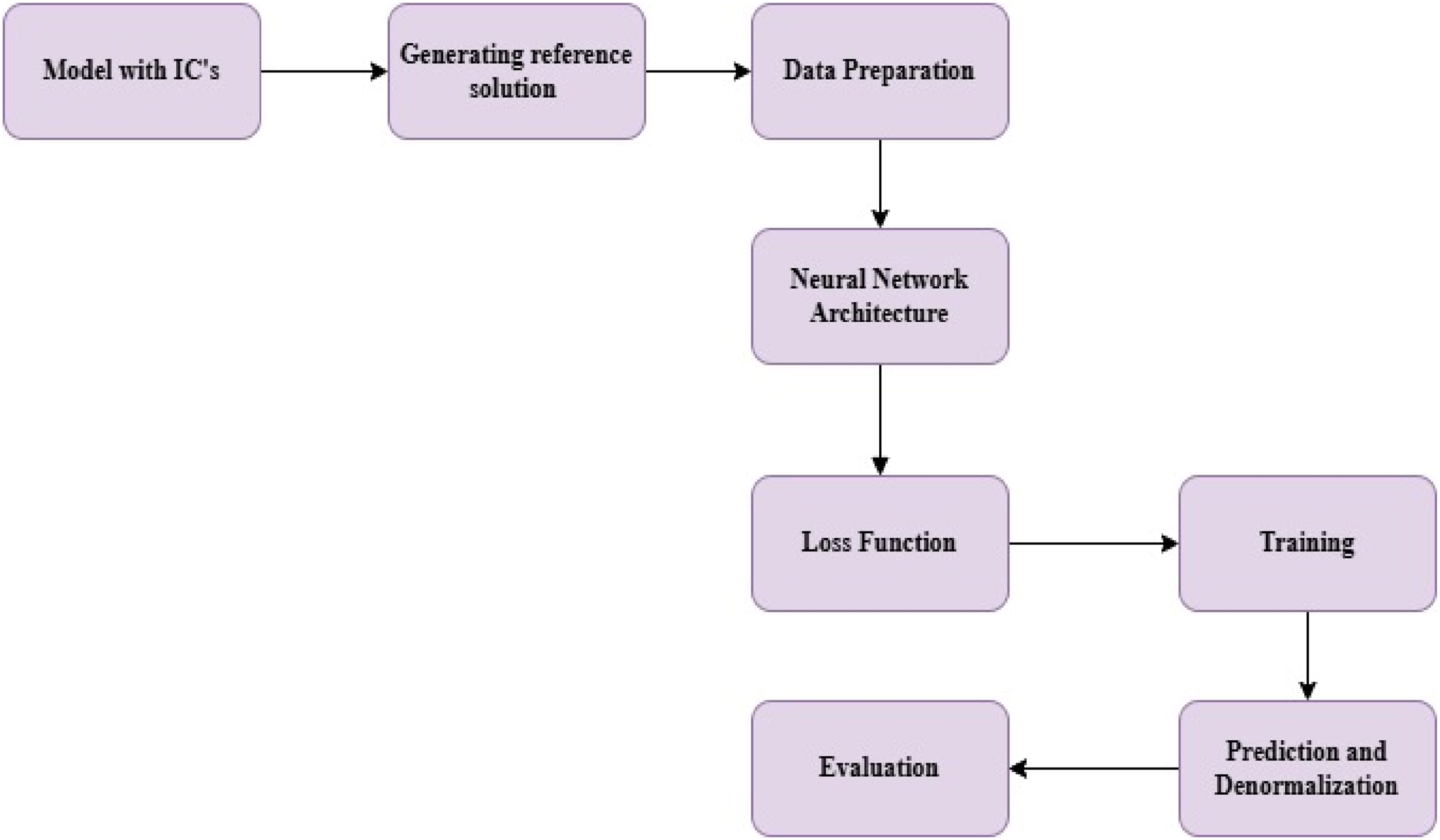
To further understand the proposed methodology, we’ll go over each step in the flowchart.
Generating reference solution
The governing system of ODEs is numerically integrated using the standard fourth-fifth order Runge–Kutta-Fehlberg method (RK45).
Let
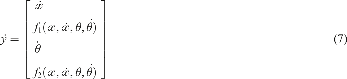
For the time span
Data preparation
The data preparation stage is a key step in training (PINN). It comprises developing a high-resolution reference solution through traditional numerical integration, standardizing all variables enhances the stability of training, and creating input-output pairs for supervised learning.
The PINN is trained using the mapping between time t and the vector:

Data normalization
Z-scores have been utilized to standardize input and target data, ensuring stability during neural network training:

Following training, predictions are denormalized and transformed to physical units.
Neural network architecture
In that phase, a deep neural network (DNN) is used as a surrogate model to approximate the solution of the system of ODEs. The architecture consists of a fully connected feedforward network with four hidden layers, each containing 256 neurons, which utilize the Tanh activation function to introduce nonlinearity. The input layer receives a single scalar—the normalized time t—and the output layer generates a 4-dimensional vector demonstrating the estimated state of the system at that moment
Loss function
The loss function in PINN plays an essential role for helping the neural network to learn each of the observed data and the basic physical rules that control the system. In this implementation, the total loss consists of two components:
Data loss: The mean square error (MSE)
This part ensures that the neural network output is approximately matched by the reference solution provided by RK45. It is used to minimize the difference between expected and true values of state variables during training. The mathematical formula of the MSE is ref 24:

Physics-informed loss
This part integrates the structure of the governing differential equations immediately into the training phase. It restricts any deviation from the anticipated physics by considering whether or not the predicted dynamics obey the ODEs at each time point. It is used to ensure that the learned solution adheres to fundamental physical rules, even in domains where no labeled data is provided. Let:

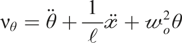
Then the physics loss is denoted by

We establish a weighted total of the two loss components in order to integrate the knowledge from both the physics and the observed data defined as:

Training
PINN implementation’s training process is developed in order to guarantee the model learns the system’s fundamental physics as well as the dynamics that exist. This process is a two-phase training approach in which the neural network learns to fit the reference data first, and then uses the physics-informed loss to refine its predictions. The first phase is Numerical Data Pre-training, where we adopt the RK45 reference solution (approximately 5000 epochs). The second phase is fine-tuning with physics Loss, where physics residuals are used to increase physical consistency and precision (5000–10,000 epochs of duration). We used the AdamW optimizer with a learning rate of 10−3 during pre-training, which was reduced to
The evaluation phase is the last and most important phase in the PINN process. It indicates how effectively the trained model captures the system’s dynamics, both statistically and qualitatively. This stage includes as follows: Comparing PINN estimations to the reference RK45 solution, presenting time series plots and phase portraits, and calculating error metrics (e.g., MAE and RMSE).
Results and discussion
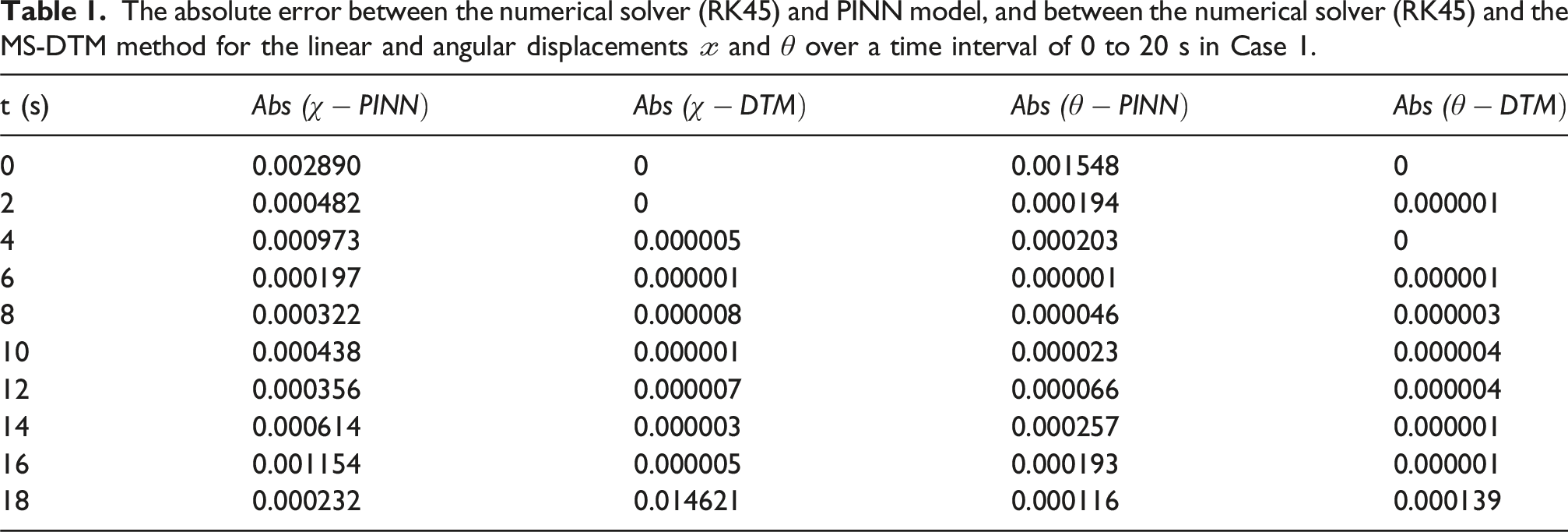
The absolute error between the numerical solver (RK45) and PINN model, and between the numerical solver (RK45) and the MS-DTM method for the linear and angular displacements
The absolute error between numerical solver (RK45) and PINN model, and between numerical solver (RK45) and MS-DTM method for the linear and angular displacements
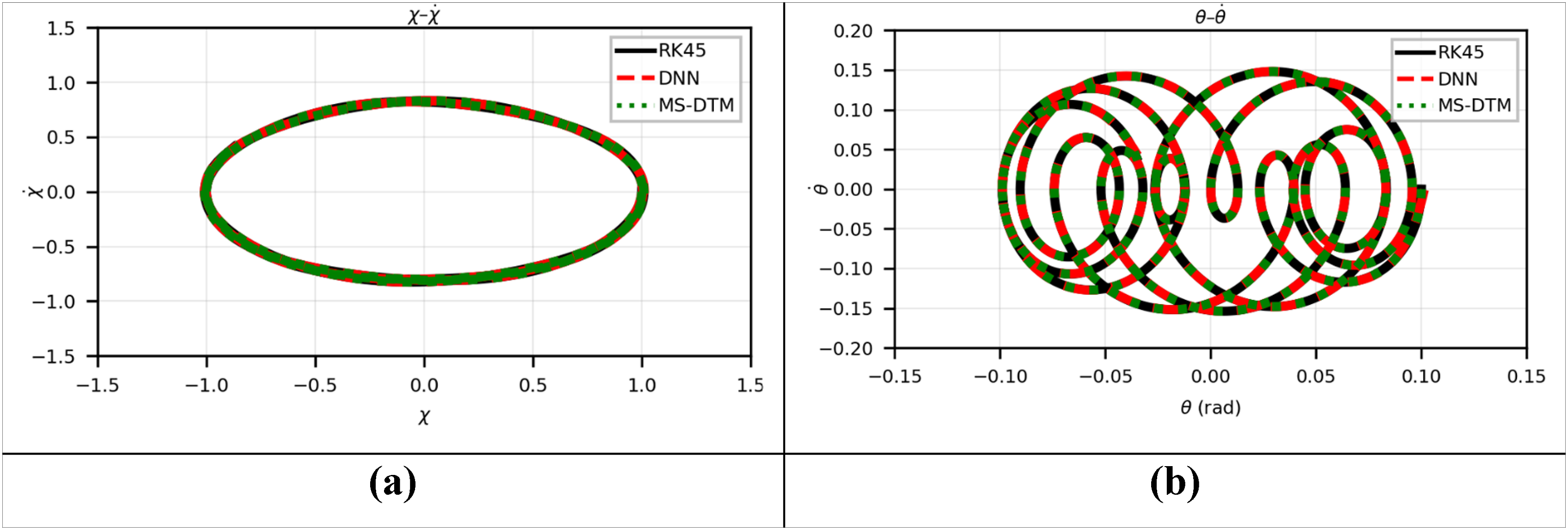
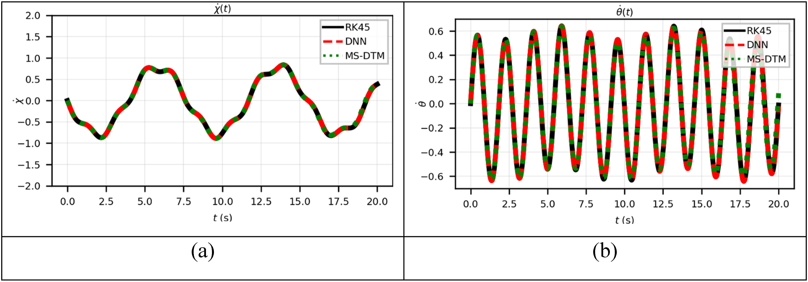
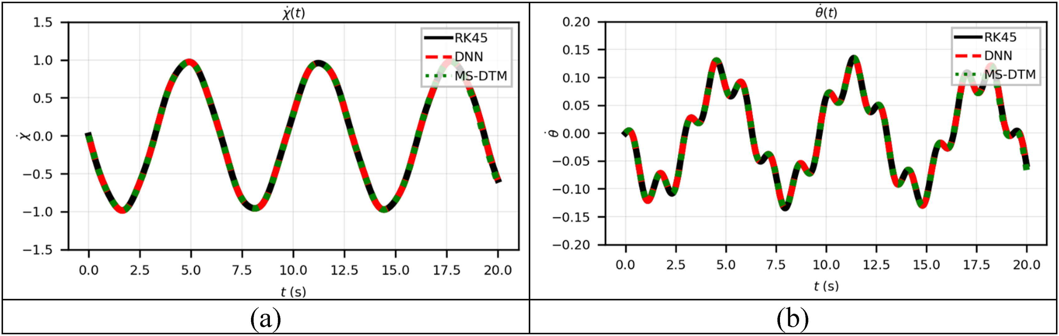
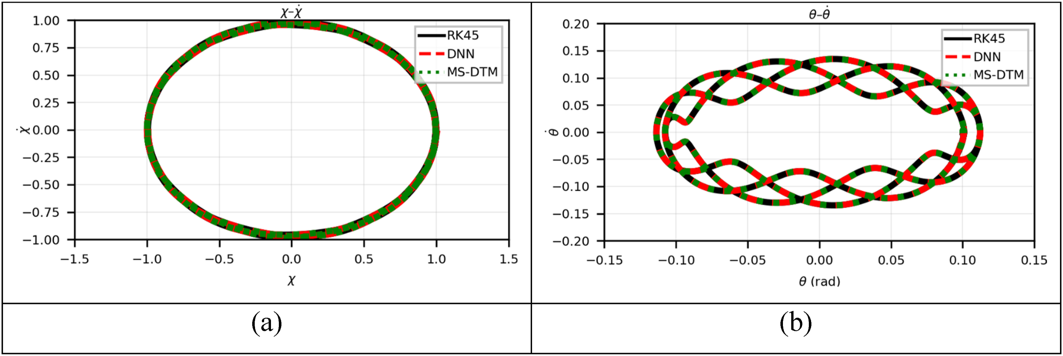
Case 1: Here the following initial conditions will be considered
Table 1 presents the numerical and PINN model results for the linear and angular displacements
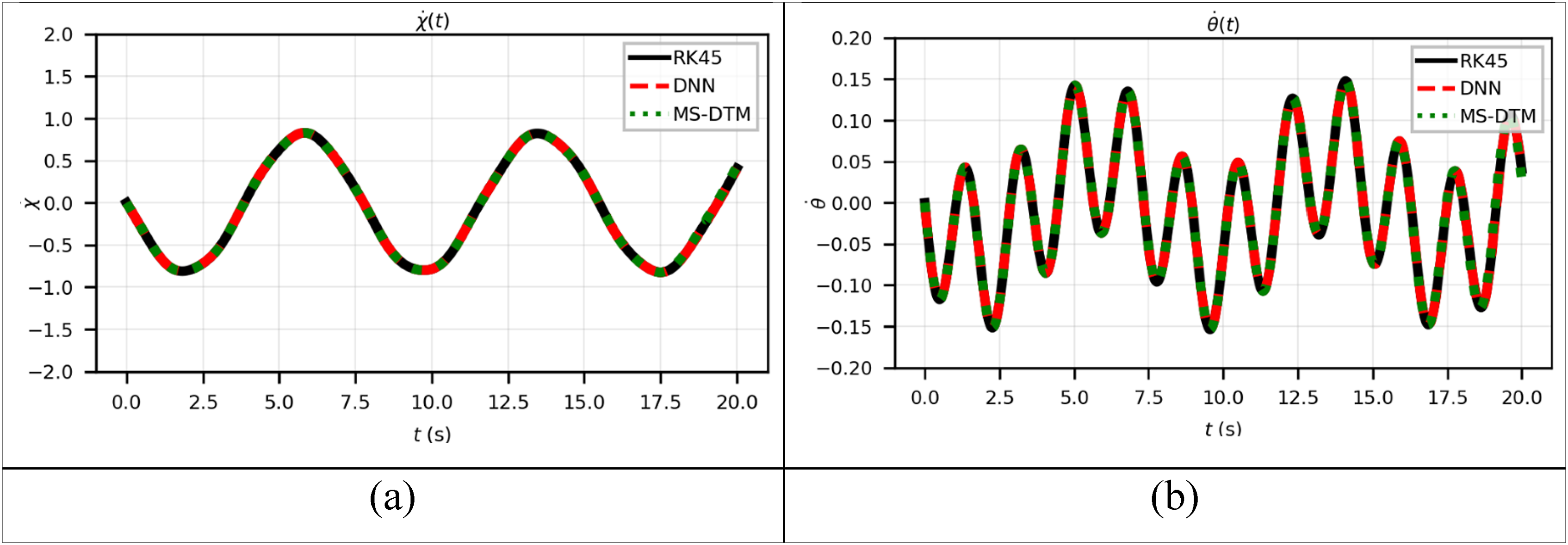
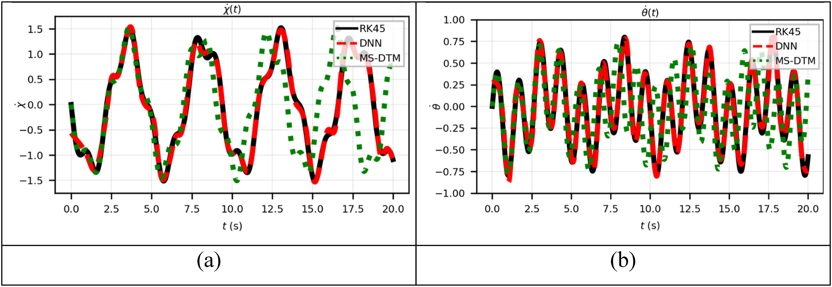
Case 1’s simulations show bounded and periodic motion, with linear and angular displacements (a) Plot of (a) Plot of (a) Phase portrait of 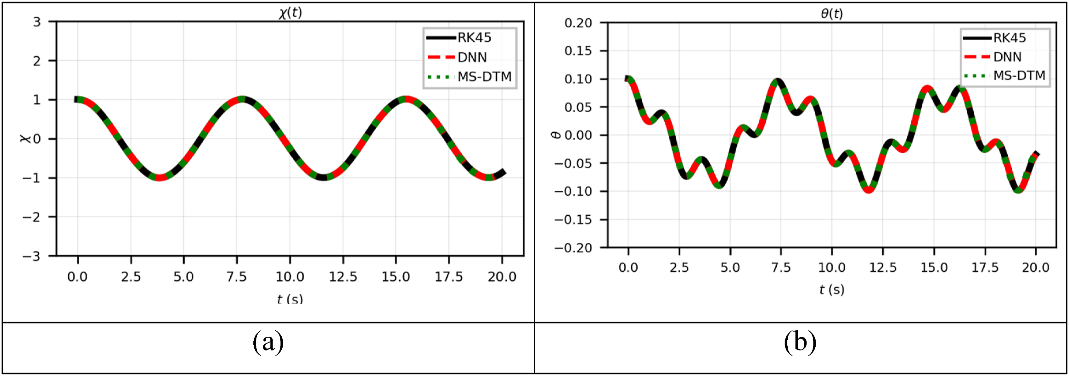
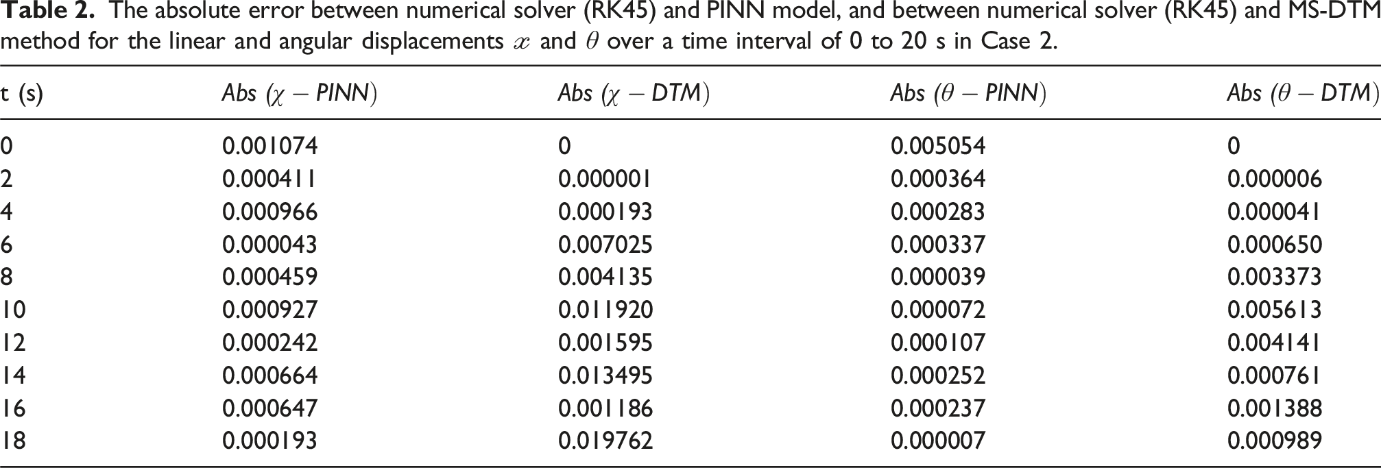
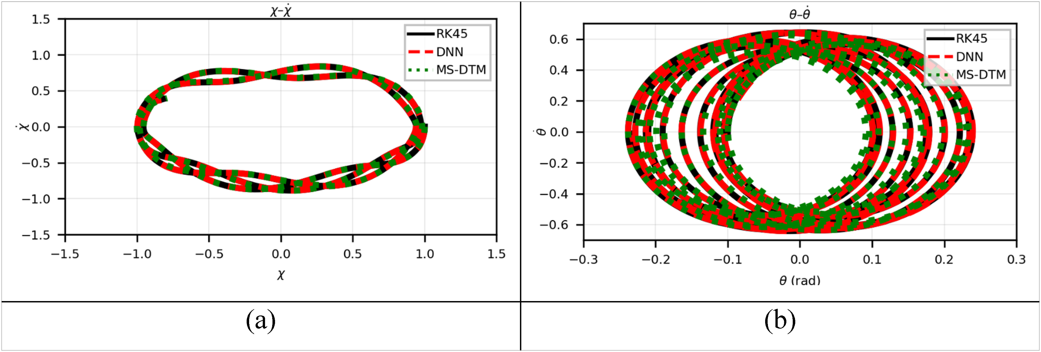
Case 2: Here the following initial conditions will be considered
Table 2 documents simulation results for Case 2, where a more asymmetric initial condition introduces greater energy into the system. Absolute errors in φ1 and φ2 are reported. Compared to Case 1, the surrogate model maintains good agreement with the numerical results, although amplitude discrepancies become slightly more pronounced due to the increased nonlinearity. The
Despite increased system energy and complexity, absolute errors in
A slightly different initial condition is used in Case 2, resulting in observable amplitude and frequency alterations. Figures 6 and 7 demonstrate that (a) Plot of (a) Plot of (a) Phase portrait of 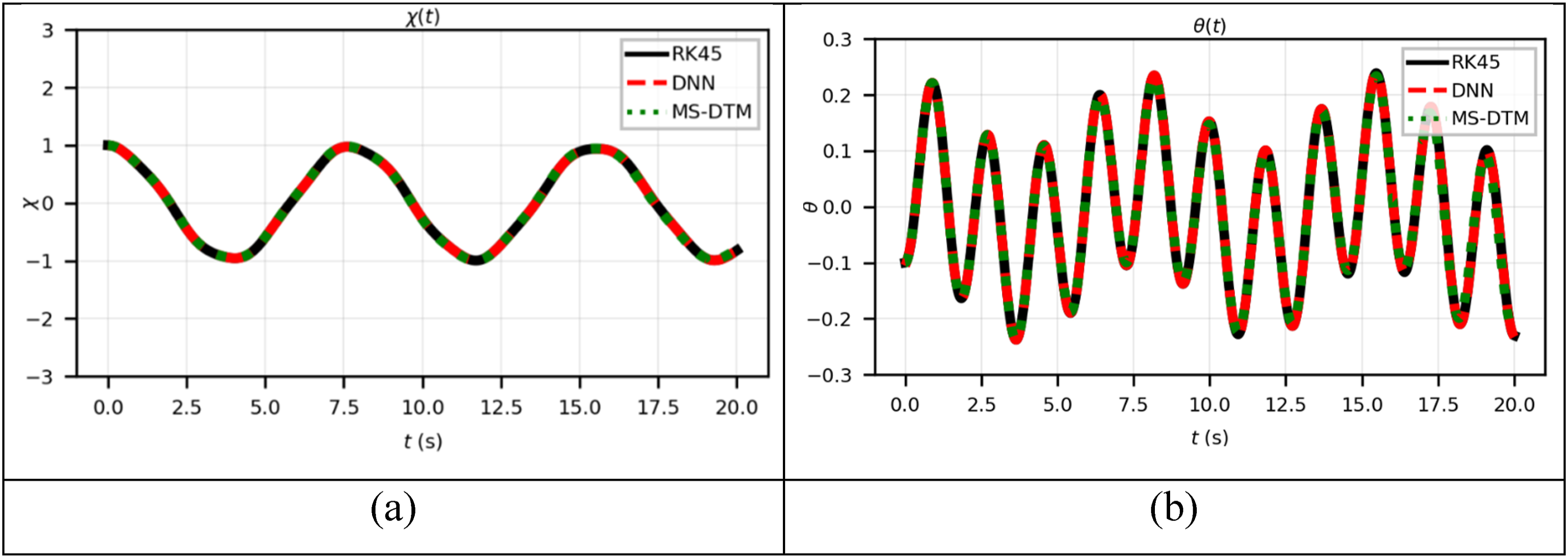
Case 3: Here the following initial conditions will be considered
The absolute error between numerical solver (RK45) and PINN model, and between numerical solver (RK45) and MS-DTM method for the linear and angular displacements
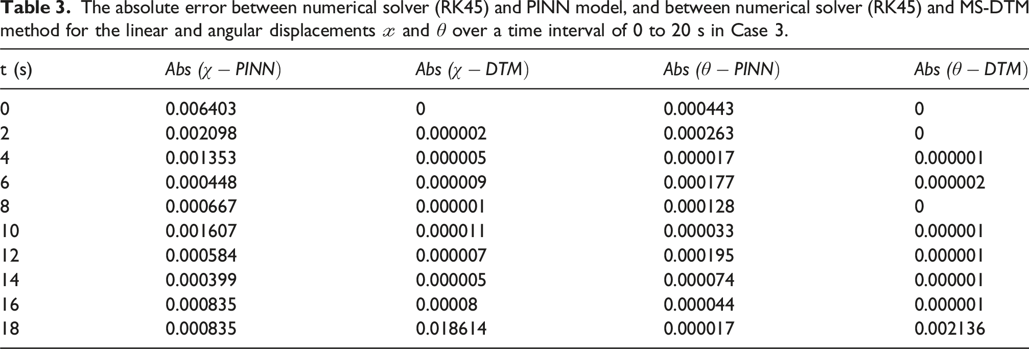
The absolute error between numerical solver (RK45) and PINN model, and between numerical solver (RK45) and MS-DTM method for the linear and angular displacements
The absolute error between numerical solver (RK45) and PINN model, and between numerical solver (RK45) and MS-DTM method the linear and angular displacements
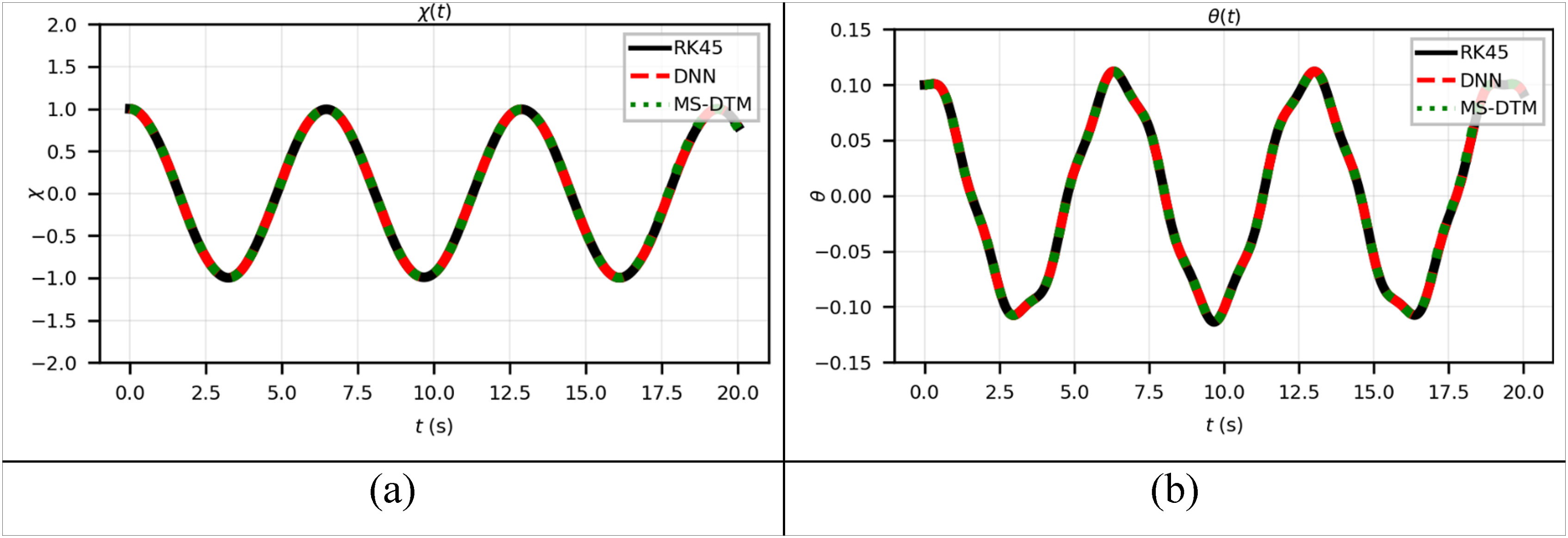
(a) Plot of
(a) Plot of
(a) Phase portrait of
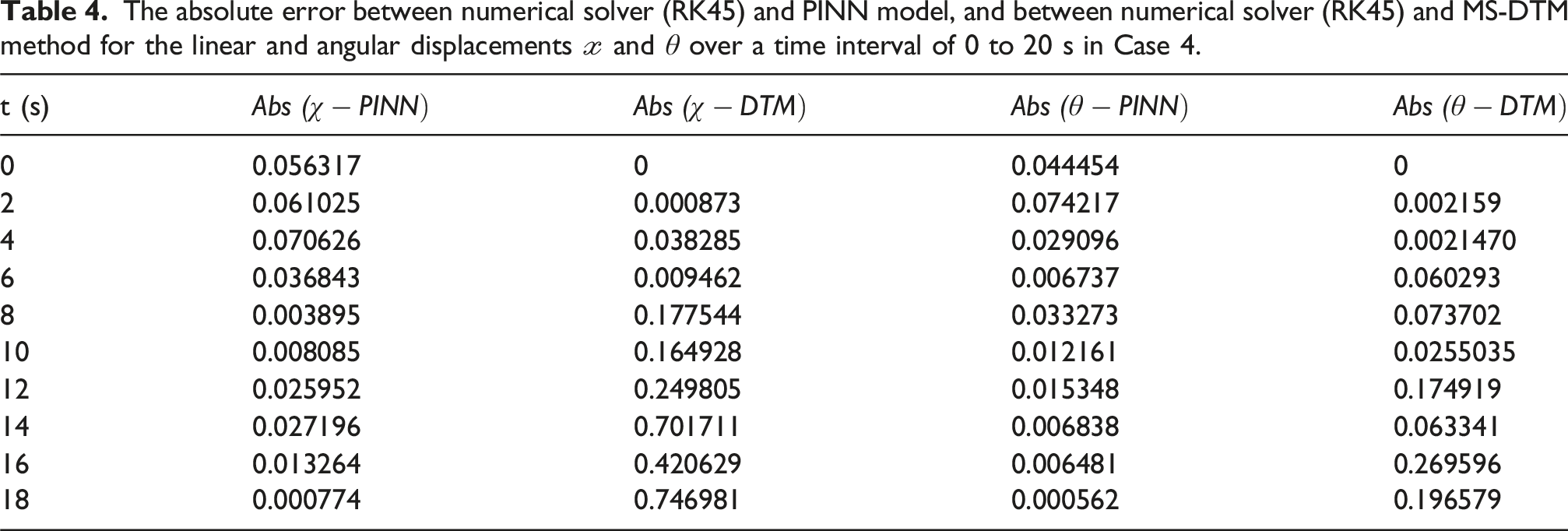
Case 4: Here the following initial conditions will be considered
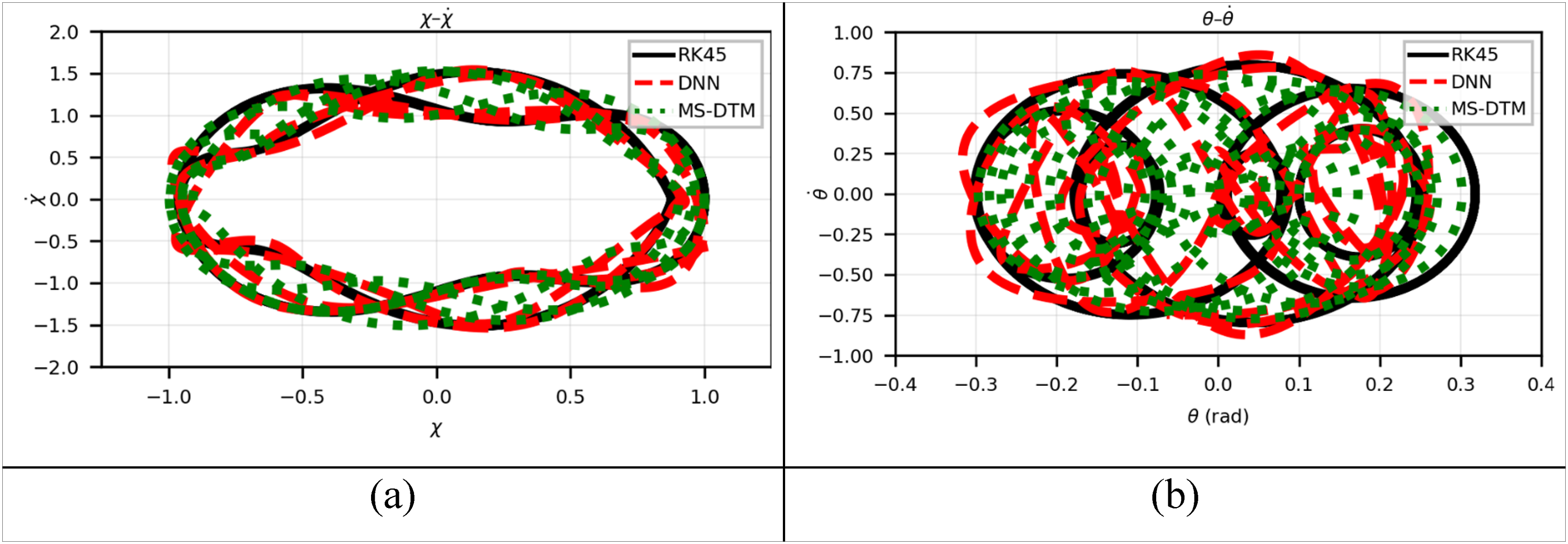
Furthermore, a higher-energy domain with significant initial excitation is investigated in Case 4. Figures 12 through 14 illustrate how the response becomes noticeably nonlinear, exhibiting irregular oscillation profiles and frequency shifts. The phase pictures diverge from classical structures and show out-of-phase interaction between (a) Plot of (a) Plot of (a) Phase portrait of 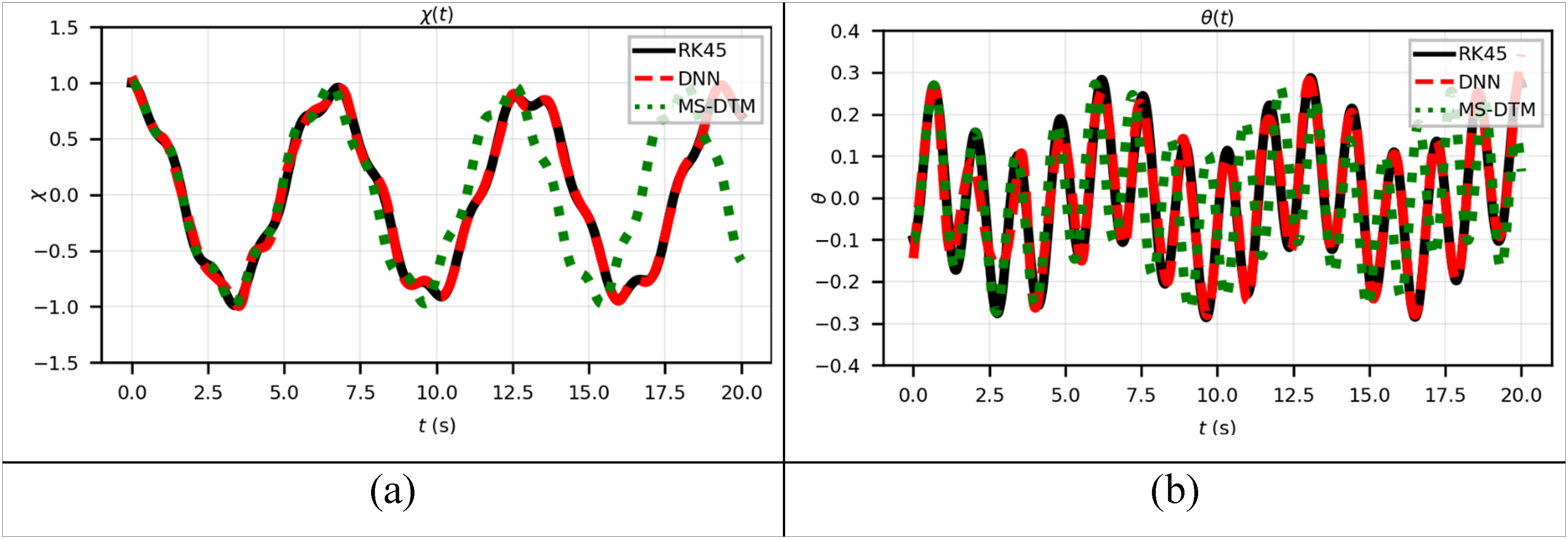
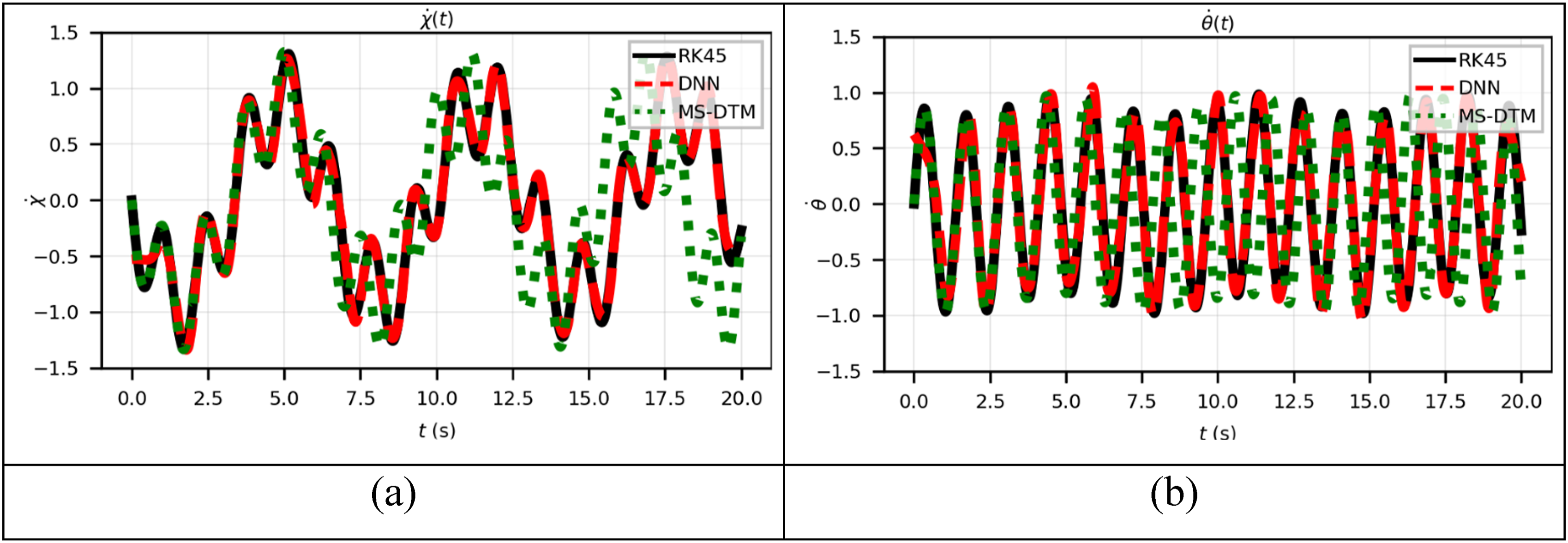
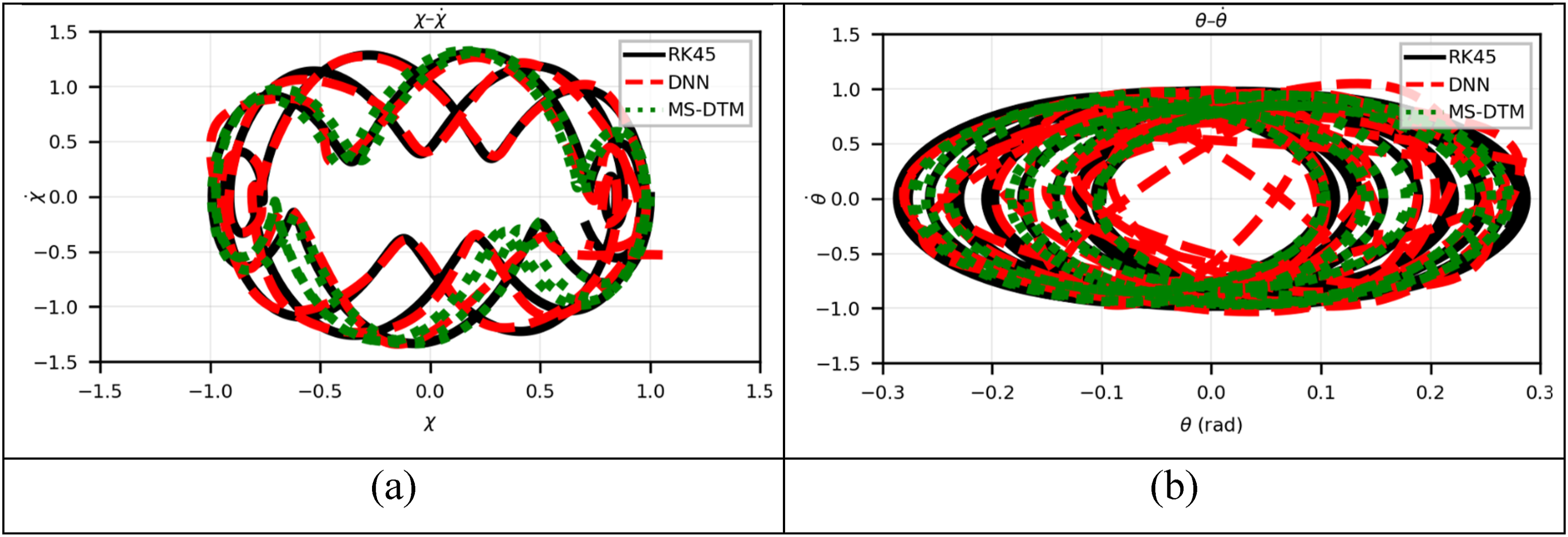
With great accuracy and generality across all situations, the PINN model accurately approximates the overall evolution of the dual-spring pendulum system. When compared to standard numerical solvers, the model confirms its applicability in modeling complex mechanical systems by retaining phase space structure, physical consistency, and long-term trajectory accuracy.
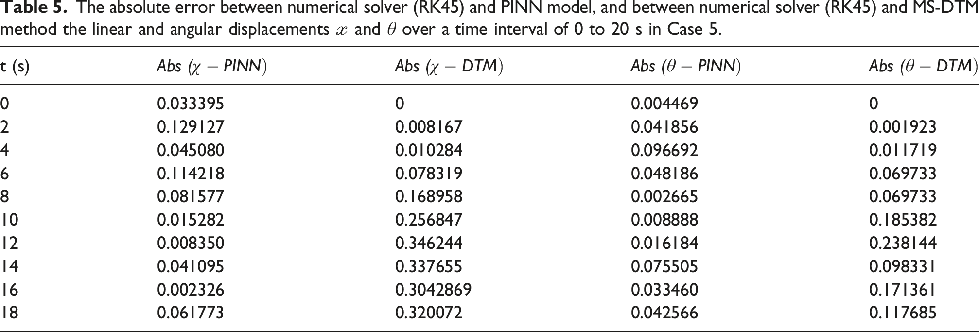
Case 5: Here the following initial conditions will be considered
Lastly, in Case 5, the dual-spring pendulum is subjected to a strong initial excitation, producing highly nonlinear and irregular oscillations, as shown in Figures 15 and 16. The time responses of (a) Plot of (a) Plot of (a) Phase portrait of 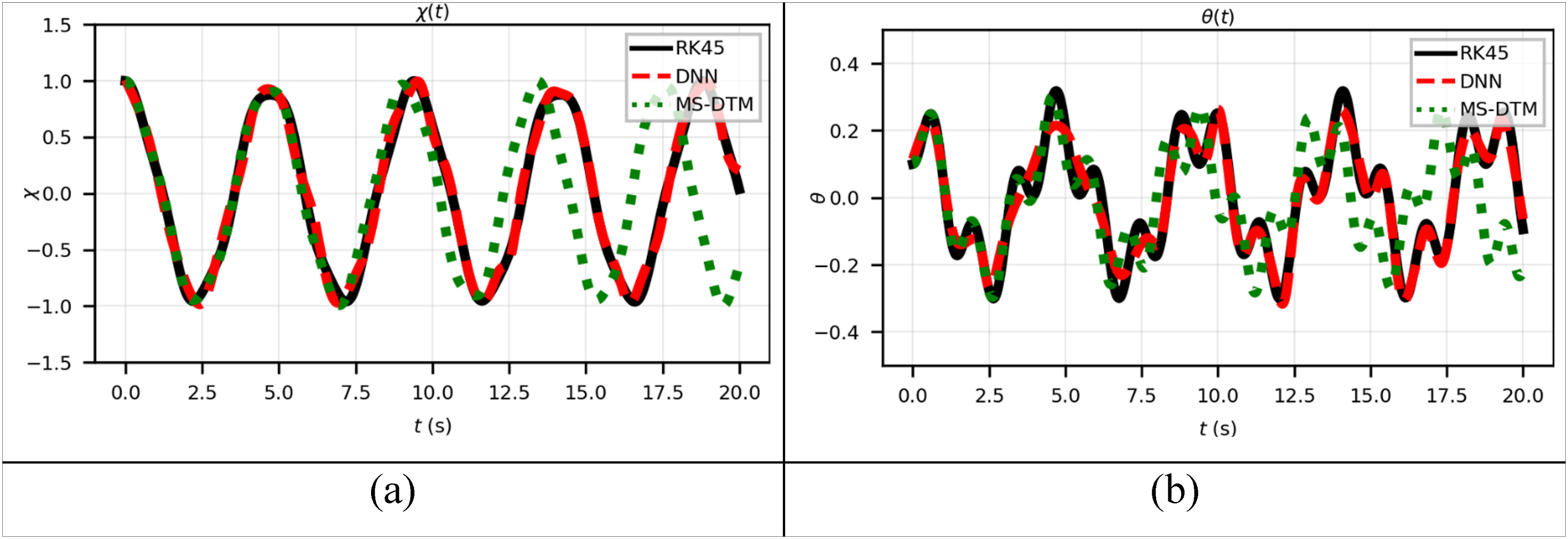
Conclusion
This study presented a comprehensive analysis of the dynamic behavior of a dual-spring pendulum system by integrating Lagrangian mechanics, numerical simulations, and physics-informed neural networks (PINNs). The results demonstrated that the surrogate model is capable of accurately reproducing both linear and nonlinear oscillatory responses, maintaining strong agreement with the reference RK45 solutions across a wide range of initial conditions. At low energy levels, the system exhibited nearly harmonic motion with bounded phase portraits, while higher-energy cases revealed frequency modulation, quasi-periodicity, and nonlinear mode coupling. Even under such complex regimes, the PINN framework preserved phase space structure and outperformed the MS-DTM method, ensuring reliable long-term predictions. These findings underscore the effectiveness of combining data-driven learning with physics-based constraints, providing an efficient and interpretable framework for modeling coupled nonlinear oscillators. Future extensions may incorporate damping, external forcing, or higher degrees-of-freedom, thereby broadening the applicability of the proposed approach to engineering and physical systems that require real-time prediction and control.
Looking ahead, a promising extension of this work is to study the fractional-order formulation of the dual-spring pendulum system. Fractional derivatives, which naturally incorporate memory and hereditary effects, provide a powerful framework for describing real-world mechanical and physical processes that are not fully captured by classical integer-order models. Exploring fractional dynamics could reveal new insights into energy dissipation, anomalous oscillations, and long-term stability of the system, while also testing the adaptability of PINNs to fractional differential equations. Such an approach would broaden the theoretical foundation of this research and enhance its applicability to complex physical and engineering problems.
Footnotes
Acknowledgments
The authors Raghad Eid, and Jihad Asad would like to thank Palestine Technical University – Kadoorie for supporting them during this research.
Funding
The authors received no financial support for the research, authorship, and/or publication of this article.
Declaration of conflicting interests
The authors declared no potential conflicts of interest with respect to the research, authorship, and/or publication of this article.