Sage Journals: Discover world-class research

Abstract

Machine learning (ML) methods are becoming more prominent in blast engineering applications, with their adaptability to new scenarios and rapid computation times providing key benefits when compared to empirical methods and physics-based approaches, respectively. However, ML approaches commonly used for blast analyses are regularly provided with inputs relating to domain-specific parameters, restricting their use beyond the initial problem set and reducing their generality. This article presents the ‘Direction-encoded Neural Network’ (DeNN); a novel way to structure an Artificial Neural Network (ANN) to predict blast loading in obstructed environments. Each point of interest (POI) is represented by the proximity to its surroundings and the shortest travel path of the blast wave in order to prime the network to learn the underlying physics of the problem. Furthermore, a bespoke wave reflection equation creates a zone of influence around each point so that obstacles are only captured in the network’s inputs if they would alter the path of the wave. It is shown that the DeNN can predict peak overpressures with mean absolute errors ∼5 kPa for unseen, complex domains of any shape or size, when compared to the results from physics-based numerical models with ∼30 times the solution time of the DeNN. The network is used to develop maps of likely human injury following detonation of a high explosive in an internal environment, with eardrum rupture levels being correctly predicted for over 93% of unseen test points. It is therefore highly suited for use in probabilistic, risk-based analyses which are currently impractical due to excessive computational cost.

Keywords

Artificial neural network machine learning human injury physics informed computation time

Introduction

Understanding how an explosion will impact its surroundings requires an understanding of how the blast wave travels and interacts with obstacles. In contrast to physical experiments, Finite Element (FE) and Computational Fluid Dynamics (CFD) numerical solvers allow for a physics-based approach to model these processes without being restricted by data capture limitations.

Primarily used as deterministic tools, these numerical models produce a single set of outputs from any number of monitoring locations in a given domain. However, it is argued by Netherton and Stewart (2016) that this does not account for the variability and uncertainty associated with explosive loading, including variable charge locations, compositions and atmospheric conditions. Therefore, focus should be placed on risk-based design, utilising probabilistic approaches and variable input combinations that provide a more robust assessment of the risk posed to a given target. Clearly, such analyses require significantly more computational resources than their deterministic counterparts.

This conclusion has sparked a number of recent studies to adopt probabilistic frameworks, including structural response assessments of masonry panels, bridge piers and sacrificial glazing subjected to blast loads (Seisson et al., 2020; Lv et al., 2022; Rebelo and Cismasiu, 2021). Whilst these assessments can be conducted with experimental results or parameter rich numerical models, Seisson et al. (2020) notes that the availability of a suitable single degree of freedom model for their study helped to drastically reduce computation times. Coupling this with blast loads being represented by triangular pressure profiles, the authors were able to evaluate 10,000 unique models to assess the influence of changing material properties on the failure probability of masonry panels.

The benefits of fast running engineering models (FREMs) are therefore clear when considering the need to simulate so many unique combinations of inputs in larger frameworks that help to develop robust understanding of the threat being posed. However, these models are not yet available for all applications that would benefit from a risk-based approach. Most notably, in the analysis of internal environments, studies by Gan et al. (2022) and Alterman et al. (2019) adopt physics-based numerical models to simulate the propagation of a blast wave throughout internal domains, leading to only 20 and 100 models being evaluated respectively. It was noted by Alterman et al. (2019) that the use of 100 CFD simulations was suitable for each threat scenario as fatality risk convergence was observed. A similar conclusion is made by Marks et al. (2021), where a comprehensive probabilistic analysis of a T-junction subjected to a vehicle-borne improvised explosive device (VBIED) is detailed. Still, in both of these studies, only a select number of charge sizes and locations are considered, and it cannot be known when risk convergence will be achieved. A suitable FREM would eliminate the chance of not observing convergence whilst also enabling an expanded range of threats to be analysed, with limited additional computation expense, to develop a more robust understanding of the risk.

An example tool that is commonly used when developing new rapid analysis methods is Artificial Neural Networks (ANNs). Comprised of a number of neurons and connections enabling information to be passed between a series of layers, in their simplest form, these networks learn from datasets of example input and output combinations to emulate the results of complex physical processes. When fully trained, they are able to generalise complex problems with multiple variables to generate new predictions for unseen inputs, provided that they are within the bounds of the inputs in the training data.

Multi-layer perceptrons (MLPs) are among the most common type of ANNs and have been shown to be successful in predicting values associated to various task-specific blast scenarios. Most notably work by Remennikov and Mendis (2006), Remennikov and Rose (2007) and Dennis et al. (2021) shows how relatively basic network structures can result in prediction-target correlations $(R_{t}^{2})$ over 0.99 for various blast parameters on city streets, behind blast barriers and in enclosed rooms, respectively.

Recent studies have demonstrated the advantages of using different network types and ML tools over the more commonly used MLP. For instance, 3-dimensional convolution neural networks, typically used in image processing, have been applied to predict peak pressure between buildings with relative errors of less than 7% when compared to equivalent numerical model outputs (Kang and Park, 2023). Similarly, transformer neural networks have shown relative errors of less than 3.5% and 14% for predictions of Boiling Liquid Expanding Vapour Explosions (BLEVEs) in free air and around rigid obstacles (Li et al., 2023a, 2023b). These adapted ANNs outperform MLPs when modelling the complexities associated with explosions and wave propagation, and a similar conclusion is reached by Zahedi and Golchin (2022) when using a gradient boosted decision tree to evaluate protruded structures. However, it is important to note that these conclusions require further exploration to assess more varied applications, data processing approaches, amounts of training data, and hyperparameter restrictions.

Artificial Neural Networks are therefore proven to be highly effective in predicting blast loads, but their application is often limited to very specific scenarios due to the nature of task-specific input features and training data. For example, in the study by Dennis et al. (2021) the authors developed an MLP that could predict peak specific impulse on a 2D plane for a charge size of 3–10 kg located within a specific rectangle of a 10 × 7 m domain with around 10% error. Inputs from outside of these ranges would rely on the network’s ability to extrapolate based on the relationships it derived during the training process. Yet, without the application of transfer learning, where a network is attached to additional inputs to effectively scale its output to suit another problem, neural networks cannot reliably predict outside of these ranges (Pannell et al., 2022a).

In addition, Figure 1 shows how the approach developed by Dennis et al. (2021) assigns inputs to the network for each prediction point relative to the user-defined origin of the domain. By providing the charge and point of interest (POI) location to the network, a prediction is made with details of the domain size and boundary conditions being embedded into the architecture of the ANN during the training process. A change in these conditions therefore renders the developed network unusable, with the user being required to develop a new tool or conduct additional CFD analysis if, for example, they wanted to evaluate the effect of a blast barrier on the output.

Figure 1.

Previously developed approach to blast wave analysis using artificial neural networks (Dennis et al., 2021). Reference to the prediction point and charge are made to a user-defined origin.

This paper introduces the ‘Direction-encoded neural network’ (DeNN), a novel application of ANNs that leverages the underling physics and utilises an input pattern representing the relevant domain geometry and charge location in relation to each individual prediction point. Hence, removing the need for information to be encoded in the tuned network parameters with little generality. As mentioned previously, various ML tools could provide the most accurate predictions for the obstructed environment scenarios discussed in this article. However, to show the importance of feature engineering compared to the approach taken by Dennis et al. (2021), an MLP is used. The novel developments that are discussed could be applied to any ML approach to explore the potential of improving the predictive performance further.

Throughout the remaining sections, the numerical solver, Viper::Blast, is experimentally validated for use in generating the training dataset before the DeNN is introduced, tested and applied to an assessment of human injury that aims to display its flexibility in use.

Numerical modelling

Introduction

The numerical solver Viper::Blast (herein referred to as Viper) is a CFD solver that is founded upon the theoretical framework established by Wada and Liou (1997) and Rose (2001), using the AUSMDV numerical scheme to solve the inviscid Euler equations. It has a wide range of applications in a number of recent studies including an air blast variability analysis, the evaluation of multiple simultaneously detonated charges and the evaluation of explosions at the opening of a mine (Marks et al., 2021; Zaghloul et al., 2021; Remennikov et al., 2022).

Detonations of explosives can be performed in Viper using the Jones–Wilkins–Lee (JWL) (Lee et al., 1968) or Ideal Gas (IG) methods. It is noted in the manual of the solver that the JWL approach is more suited to scenarios where the expansion of the detonation products needs to be more accurately replicated, such as in the near-field, or if blast-obstacle interaction close to the source is expected. Whereas, IG simulations require reduced computational effort making them more suited to solving far-field problems.¹

Viper also allows simulations to be conducted in 1D, 2D or 3D, with data mapping capabilities between each option. Remap files can be generated at termination of a model or when a gauge is triggered (records a non-ambient value) in the parent domain. This enables the Branching Algorithm to work seamlessly with the solver (Dennis et al., 2022), since repeat calculation steps are removed from the simulation process of a batch of similar models though informed data mapping that requires remap files to be generated at specified locations. However, for this study, remapping is used to simulate the initial detonation of each blast in 1D, with a small cell size, before mapping into a 3D domain that uses a coarser mesh to reduce computation time.

To identify a suitable solving method and cell sizes for both 1D and 3D phases, the following sections provide a mesh sensitivity study and mapping scale factor analysis. The former determines a suitable approach through comparisons to the Kingery and Bulmash (KB) method (Kingery and Bulmash, 1984), whereas the latter compares results from a 3D domain to experimental trails of PE4 hemispheres, using various charge sizes and stand-off distances.

All simulations in this article were performed using Viper version 1.20.6a on a computer that utilises a NVIDIA T1000 dedicated graphics card with a CUDA compute capability of 7.5, in addition to 16 GB of system RAM and an Intel Core i7-10700 processor.

Mesh sensitivity

A mesh sensitivity analysis has been performed to identify the cell size and solving method required to preserve the initial release of energy when simulating the detonation of an explosive in a 1D phase. This is achieved by observing convergence of the outputs from a series of gauges in a 1D Viper model with comparisons made to the KB method (Kingery and Bulmash, 1984).

PE4 is chosen as the explosive since experimental comparisons provided in the next section will use this compound. Similarly, hemispherical charges are modelled to enable continuity throughout the validation process. Both the JWL and IG solving methods are evaluated to output the incident peak overpressure and specific impulse at stand-off distances of 4 m and 8 m for a charge size of 250 g.

The built-in properties provided in Viper for PE4 are only suitable for the JWL solving approach. However, as discussed by Bogosian et al. (2016), C4 and PE4 are nominally identical, and so the C4 model can be used for IG simulations. Additionally, each charge is modelled as twice the hemispherical mass to account for how the 1D solver (spherically-symmetric) does not include a reflecting ground surface. Viper input parameters for this process are shown in Table 1.

Table 1.

Viper::Blast training model parameters.

	Parameter	Value	Unit
Generic	Pressure	101,325	Pa
	Temperature	288	K
	CFL: 1D	0.5
	CFL: 3D	0.4

PE4 (C4): IG	ρ ₀	1580	kg/m³
PE4 (C4): IG	E ₀	6.06E6	J/kg

PE4: JWL	ρ ₀	1576	kg/m³
	E ₀	8.698E6	J/kg
	A ₁	9.5929E11	Pa
	R ₁	5.616
	A ₂	4.914E9	Pa
	R ₂	1.804
	ω	0.136
	D _CJ	7929	m/s
	F_v__min	7929	m/s
	P _CJ	2.4E10	Pa

Figure 2 shows that as the cell size reduces, the peak pressure and specific impulse of both solving methods begin to converge on the KB predictions. Since the KB method uses semi-empirical equations derived from tests using TNT instead of PE4, an equivalency factor of 1.2 is used to convert the mass of PE4 to an equivalent mass of TNT when predicting these values (Rigby and Sielicki, 2014).

Figure 2.

Results from mesh sensitivity analysis and evaluation of IG and JWL detonation models for PE4.

At both stand-off distances, the peak overpressure output from Viper is within 10% of the KB output as the cell size approaches 0.005 m. However, specific impulse is routinely under predicted, in particular when using the IG simulation. Convergence of both methods occurs with a cell size of 0.002 m, providing around 20 cells across the charge radius.

Cell size in 3D

When mapping from 1D to 3D, an increased cell size is required to prevent prohibitively large computation times. However, cell sizes too large will result in rounding of the pressure traces leading to inaccurate estimates of the blast parameters.

In this section, Viper models featuring 250 g PE4 hemispherical charges are compared to experimental results obtained by Rigby et al. (2015) for the arrangement shown in Figure 3. A 1D phase is simulated to a stand-off of 2 m with a cell size of 0.002 m to provide ∼21 cells across the charge radius. This initial detonation is mapped into a series of 3D domains featuring differing cell sizes to identify a suitable increase.

Figure 3.

Experimental arrangement and gauge positions (Rigby et al., 2015).

Experimental peak values are taken from curves that were fit to the pressure traces of gauge 1 (G1) to negate the effects of sensor noise and variation. The blockwork wall that the gauge is mounted to is represented in Viper as a non-reflecting boundary.

As shown in Figure 4, for stand-off distances of 4 m and 8 m the computation time greatly increases as the cell size decreases below 0.016 m. There is also minimal improvement in the peak pressure and specific impulse comparisons below this point. The peak overpressure may be a function of the number of cells in the domain, however, there still appears to be a minimum cell size that should be provided to prevent a loss of resolution that reduces the peak readings. Here, this is identified to be 0.02 m. Conversely, the predictions of the peak specific impulse are consistent with all cell sizes, suggesting that it is the initial burst energy, handled in the 1D phase, that is more important to preserve for this parameter.

Figure 4.

PE4 validation with 250 g hemispherical charges and gauges placed at 4 m and 8 m stand-offs.

Far-field experimental validation

The previous two sections have shown that in order to preserve the peak overpressure and specific impulse of a simulation, the 1D cell size of the Viper models should provide at least 20 cells across the charge radius and that the 3D cell size should not exceed 20 mm. To verify these findings, and assess the ability of Viper to produce reliable pressure-time histories, three additional comparisons are made against existing experimental data.

Figure 5 shows the pressure-time and specific impulse-time histories for stand-off distances of 2, 4 and 6 m and charge sizes of 250 and 350 g. In all cases, IG Viper models have been simulated with 2 mm and 16 mm cells in the 1D and 3D phases, respectively. The time of arrival of the Viper traces were matched to the experimental records.

Figure 5.

PE4 overpressure-time histories for various PE4 hemispherical charge sizes and stand-offs. (a) 2m 250 g. (b) 4m 350 g. (c) 6m 350 g. Time scales are adjusted so that the arrival times of the Viper models match the experiments.

Agreement is generally good for all stand-off distances with suitably shaped traces and peak values. The secondary shock is not predicted accurately, however, this is a known drawback of CFD analyses (Rigby and Gitterman, 2016). Overall, Viper is shown to produce reliable results when adhering to the cell size requirements of the 1D and 3D simulation phases.

In the following section, the Direction-encoded ANN is introduced, trained and tested. The models used in each of these development stages will be simulated in accordance to the output of this mesh sensitivity and validation study.

The Direction-encoded Neural Network (DeNN)

Introduction

Considering the various mechanisms associated to how blast waves interact with obstacles, including channelling, clearing and reflection, it is clear that the cause of varied blast properties is linked to the path that the blast wave must take to reach a POI, rather than the shape and size of the domain or the entire topology. The DeNN’s input pattern is therefore informed by the underlying physical processes, and structured to include the shortest wave travel path and the influence of surrounding obstacles according to 16 directional ‘lasers’ on a 2D plane as shown in Figure 6.

Figure 6.

DeNN approach to blast wave analysis using artificial neural networks. Reference to the prediction point is made relative to the surroundings and the blast wave’s path.

Taking inspiration from robotic vacuum cleaners and how they navigate their surroundings, these lasers act as range finding tools that inform the ANN about the proximity of rigid surfaces around the POI. Robot vacuum cleaners use these distances to identify where they can go, where they cannot go and where needs to be cleaned (Chiu et al., 2009; Kang et al., 2014). However, here the obstruction distances are evaluated with a wave reflection equation that alters the magnitudes of each input relative to the wave travel distance, resulting in closer obstacles providing larger inputs (i.e. having a larger contribution to the signal that is processed through the network). Seeing as intersections with ambient boundaries are represented by an input of 0, this emulates the non-linear superposition of reflected blast waves and how this process increases with shock strength. Thus, physically informing the network that surfaces closer to the POI will lead to reflections that have a greater influence on the peak pressure.

The network is developed using 1 kg TNT, with the charge size being omitted from the input pattern. This allows other domains, featuring different masses or charge materials, to be compatible with the ANN by being scaled according to equivalency factors and Hopkinson–Cranz scaling laws (Cranz, 1926; Hopkinson, 1915). Additionally, the wave travel distance is calculated through shortest path analysis, where each domain is discretised into a network of nodes allowing the blast wave to be tracked from charge to prediction point. This process is also utilised by the Branching Algorithm (Dennis et al., 2022).

Input features

The feature selection process for developing the DeNN involved iterative trials of various methods that represented the POI surroundings in different ways. Each feature described in the following sections is inspired by the physical processes associated with wave propagation, helping to form a machine learning (ML) tool that understands wave interaction effects in a generalised way.

Rotating laser directions

The application of rotating laser directions results in direction 1 pointing towards the charge centre. The value of the input associated to this direction is restricted to the wave travel distance to ensure that obstacles behind the charge are not translated to the DeNN, thus having no impact on the predictions. Implementing rotating lasers is required to maintain consistent network predictions for points that are expected to have identical outputs. For example, a symmetrical domain featuring POIs behind blast panels on either side of the charge should provide the same input pattern to the DeNN. If the lasers had a fixed orientation, different input nodes would be activated (non-zero input) for each POI, likely leading to different predictions.

Superposition equation

To account for wave reflections and superposition effects, each directional input is calculated using equation (1) if a obstruction is identified by the laser. Otherwise the input magnitude is set to 0 for an ambient interaction.

Directional input = \max (Wave travel distance - Obstruction distance, 0)

(1)

where the wave travel distance is the shortest path between the charge and the POI, and the obstruction distance is equal to the distance each laser travels before encountering a rigid obstacle. An example is provided by Figure 7 to show that directional inputs 12 and 13 have an obstruction distance of 7.07 m, a wave travel distance of 9 m and a resulting directional input of 1.93.

Figure 7.

Example application of equation (1) showing directions 1, 4, 5, 8, 9, 12, 13 and 16 for clarity.

In theory, the polarity of inputs to an ANN does not affect its predictive performance as long as the network parameters are optimised through sufficient training steps and remain consistent throughout development and use. The weights and biases of the first layer of connections can be adjusted to account for positive or negative input values. However, the magnitudes of each input and their relationships do affect performance. Equation (1) enables larger or smaller interaction effects from obstacles that are closer or farther from the POI to be translated with correspondingly larger or smaller values relative to the shortest wave travel distance.

The superposition equation is inspired by how existing fast running methods utilise multiple charge superposition to model blast wave reflections, with a charge at an imaginary source behind a wall providing the wave that amplifies the predictions at rigid surfaces (Pope, 2011). In these applications, this has the effect of defining a ‘zone of influence’ around the POI such that any obstacle interactions outside of the zone are deemed to be insignificant for the peak pressure prediction, that is, acting like an ambient boundary with a 0 input. A similar concept is shown to apply to the design of continuous beams (Gallet et al., 2023).

Figure 8 provides the zones of influence for two example points in a domain. For point A, the close proximity to the charge results in a small zone of influence, showing how the blast wave will not be obstructed by the presence of obstacles outside of this region as it approaches the POI. The zone for point B is much larger since shortest wave travel path must wrap around the horizontal obstacle. The directional lasers must therefore consider obstacles that could contribute to wave coalescence along this path.

Figure 8.

Zones of influence examples showing the regions where directional inputs would be treated as ambient at stand-off distances greater than the wave travel distance in accordance to equation (1).

Multiple neural networks

When considering the peak pressure distribution through a domain featuring various obstacles, larger magnitudes of peak overpressure are often in positions where no shielding from obstacles is provided. These positions are dominated by free air blast waves that can be amplified by channelling or reflections from obstacles behind the POI, whereas POIs behind obstacles experience clearing and diffraction effects leading to reduced readings. Requiring a single neural network to learn about the processes associated with both of these regions may therefore needlessly restrict prediction accuracy. Since a distinction can be made by considering each POIs position relative to the charge, the DeNN model is applied as two separate ANNs with identical input-output structures. One network (ANN-1) is used for POIs with a direct line of sight to the charge, and the other (ANN-2) is used when an obstruction is present.

Although not done in this manuscript, separating the simple from the more complex settings in this way facilitates the implementation aspects of transfer learning. For example, ANN-1 could be replaced with simple empirical predictions, or different models to account for TNT equivalence (Grisaro et al., 2021; Pannell et al., 2022a).

Example input patterns

Figure 9 shows how some common input patterns are represented with the DeNN, with only 8 of the 16 directions included to benefit readability.

Figure 9.

Example directional inputs for various points, showing directions 1, 4, 5, 8, 9, 12, 13 and 16 for clarity. Thick black line in the directional rosette indicates direction 1.

Plot A features a wall behind the POI and so the inputs in the backwards direction are more similar in magnitude to the wave travel distance, in accordance to equation (1). The contrast with lower values in the forward positions helps the network to understand that blast wave reflection should be considered when forming the prediction. Next, plot B’s POI is shielded by a wall resulting in larger forward inputs and low backwards ones. Finally, plot C show how a POI between two rigid bodies leads to large input magnitudes in all side directions of the input pattern.

In each case, a distinct combination of directional inputs are activated, thus providing different routes for information to be passed through the DeNN’s connections when predictions are formed, ultimately allowing for differing wave processes to be represented.

Dataset development and training

Training dataset

A key part of developing a ML tool that can be useful in practice is related to the quality and quantity of training data points. To develop a suitable dataset to analyse the performance of the DeNN, 25 randomly generated Viper numerical models, shown in Figure 10, have been simulated. This aims to provide a range of unbiased blast scenarios that include obstacles positioned in a wide range of locations so that the networks can generalise from the training process and provide predictions with suitable accuracy regardless of the prediction domain.

Figure 10.

Randomly generated training models used to develop the DeNN.

The random generation process applied limits on the number of obstacles (0–5) and their size (0.01–5 m²), their shape (square/rectangle) and orientation (0° or 90° to the horizontal), and the size of the overall domain (10 × 10 m, 10 × 8 m, 8 × 10 m, 8 × 8 m). All other geometrical parameters were unrestricted.

The 1 kg TNT spherical charge was positioned at 1.5 m above a rigid reflecting ground surface in every domain with a grid of gauges also being specified at this height with regular spacing of 0.1 m. Gauges within 1.5 m of the charge were then removed as this 1.5 m sphere around the charge is a true free-air case. Standard rapid analysis methods, such as ConWep, can therefore be used if information about this region if required. Furthermore, peak overpressures are also expected to be far greater in this region than in any other part of the domain and so their removal reduces the range of values that need to be predicted by the ANNs. This will have the same impact as the specific impulse limit employed by Dennis et al. (2021), where performance was improved for predictions of lower magnitudes once the rare, especially large, values were omitted.

A potential issue with using a randomised training dataset is related to how each directional laser will be provided with a non-zero value a different number of times. The tuning of the weights and biases associated to each direction is likely to be inconsistent, resulting in symmetrically inaccurate predictions. To reduce the impact of this effect, the training dataset is mirrored so that each laser to the left of direction 1 is activated in the same number of input patterns as the opposite laser to the right of direction 1 (e.g., direction 6 opposes direction 7). Using this approach, the DeNN therefore has access to input patterns that relate to obstacles on both sides of direction 1 in equal quantities, whilst also remaining physically valid, during the training process. Overall, this methodology provides 354,554 unique data points.

The size and shape of the domains used in the training process have little effect on the ultimate performance of the DeNN due to how the inputs are derived with reference to the surroundings instead of the domain itself. It is more important to provide a wide range of target peak overpressures and a range of activated (non-zero) directional input combinations. In this case, the 25 models provide the magnitude ranges shown in Table 2. These form the allowable bounds of inputs associated to future scenarios requiring prediction. It should be noted that the low mean value associated to ANN-1’s directional inputs is caused by a large number of ambient (0 magnitude) inputs.

Table 2.

Training dataset variable statistics.

ANN num	Variable	Units	Min	Max	Mean	Std. deviation
1	Directions	m/kg^1/3	0	12.28	0.96	1.86
	Wave travel distance	m/kg^1/3	1.52	12.28	4.57	2.03
	Peak overpressure	kPa	7.99	672.34	66.30	55.38
2	Directions	m/kg^1/3	0	13.17	2.05	2.90
	Wave travel distance	m/kg^1/3	1.97	13.93	7.20	2.05
	Peak overpressure	kPa	4.72	171.89	19.31	11.01

At each gauge location, pressure histories are recorded by Viper. The peak reading is extracted and aligned with the directional input patterns and wave travel distances that are calculated using the discretised domain representation given by the 0.1 m gauge grid. The networks are trained by considering the inputs with a known target output from the validated solver. Details of the Viper models are given in a following section.

Testing models

In order to test the performance of the trained ANNs, two additional models have been simulated to enable a real world assessment of the predictive performance. These independent tests are not restricted by the aforementioned randomisation requirement and are developed with the aim of replicating some expected domain layouts that could be seen in practice. By assessing the performance for these unseen inputs, the impact that the randomised training dataset has on the generalisation capabilities can be observed.

Figure 11 provides the dimensions for both testing models, with all input parameters falling within the bounds of the training dataset shown previously in Table 2. T1 aims to test the network’s ability to predict the peak overpressure in a simple scenario with various blast panels, whereas T2 requires greater appreciation for more complex wave interaction effects, with channelling and shielding replicating a scenario more closely aligned to a cityscape layout, albeit a simple one. Both models include 1 kg TNT charges, positioned at 1.5 m above the rigid reflecting floor.

Figure 11.

Selected testing models to be used for unseen ANN performance assessment.

A key feature of both testing domains is that they do not share equal size or shape with any of the models used to form the training dataset. Seeing as the DeNN references the surroundings of each prediction point and not the domain itself, predictions can still be generated on a 0.1 m gauge grid, positioned 1.5 m above the rigid ground plane. It should be noted that it is possible for the user to change this predictive grid spacing in future use cases if required.

A large range of input patterns and corresponding outputs are generated for training, and only specific patterns will also feature in real world applications. In some cases, the accuracy may be better than expected, and in some it may be worse. For example, the average error of the network may be 10%, however, this could include a 1% average error for points being shielded, and a 30% error for those where channelling with have the largest impact on the peak parameter. By generating predictions for these specifically designed testing models, it will highlight these variations.

The schematic shown in Figure 12 presents the data splitting process used through training, with 4-fold cross validation and the two independent testing models. The final model, used to predict the testing data, is trained using all training data for the average number of steps required by the cross validation process.

Figure 12.

Representation of how data are split for K-fold cross validation during training, showing that this is independent of the two additional models that have been devised for testing the trained DeNN. Adapted from Pannell et al. (2022b).

Viper::Blast modelling

Each model in the training dataset will be simulated using the chosen numerical solver, Viper. Following its validation earlier in this article, this solver provides the functionality required to generate peak overpressure readings throughout each domain at the specified grid spacing.

Setup parameters are provided by Table 3 and in each case all boundaries are set to be ambient (transmit) aside from the rigid reflecting floor. The simulations utilise 1D–3D mapping with the 1D stage running until the blast wave has reached one cell away from this boundary at 1.499 m from the detonation point. Whilst the DeNN will predict for a 2D plane at 1.5 m elevation, it will be trained with data from a more comprehensive modelling process, carried out in 3D with a domain height of 2 m. To remove the potential influence of ambient boundary effects on the peak overpressures recorded by gauges at the boundaries, each boundary is extended by 0.5 m.

Table 3.

Viper::Blast training model parameters.

Solving method	Ideal gas
Charge size (kg)	1
Charge composition	TNT
Charge density (kg/m³)	1600
Charge energy (J/kg)	4.52 × 10⁶
Mapping	1D–3D
1D cell size (m)	0.001
1D CFL	0.5
3D cell size (m)	0.02
3D CFL	0.4
Ambient temperature (K)	288
Ambient pressure (Pa)	101,325
Termination time (s)	0.05

Network structure

With any ML application, there are a number of different hyperparameters that can be tuned to provide an optimal network structure for each unique application. For ANNs, this includes the number of hidden neurons, number of hidden layers, dropout rate and the optimiser learning rate. Conducting a grid-search to test every possible combination would be very time consuming and computationally expensive, and so for this study a range of setup variables, shown in Table 4, are fixed throughout the tuning process. Each parameter is matched to those used by Dennis et al. (2021), since this study showed that they are suitable for generating accurate predictions for a similar blast application.

Table 4.

Fixed network parameters.

Output activation function	Linear
Loss function	Mean squared error (MSE)
Training steps	500
Batch size	100
Regularisation	L2
Weight initialiser	Glorot Normal
Bias initialiser	Zeros
Cross validation folds	4

The ANNs are coded in the Python programming language using the Tensor Flow and Keras packages for ML. Training is allowed to continue for up to 500 steps unless the early stopping criteria is met. This being that there is no improvement in the validation loss (mean squared error) for 10 steps, where ‘no improvement’ includes loss variations of 1 kPa² or less. The network is only saved after each training step if it provides the best performing validation loss, replicating the process implemented by Bakalis et al. (2023). This ensures that if the training performance continues to improve despite a decline in validation performance, the weights and biases of the network are not saved. Thus, preventing overfitting and allowing for good generalisation with unseen inputs.

Four fold cross validation is utilised to ensure that the network performance is evaluated for the entire training dataset. This process involves splitting the dataset into four equal sections, with four separate networks being trained on a different 75/25 training/validation subset. Performance is reported as the mean average of all the folds so that bias in the validation data split is removed. Following cross validation, the final model is trained for the number of training steps equal to the average from all folds considering the early stopping criteria, using all the training data.

The KerasTuner is applied using the hyperband optimisation process to identify an optimal combination of the hyperparameters being trialled in this study (Li et al., 2018; O’Malley et al., 2019). Table 5 provides each variable with the associated sampling method or step size and the potential values. The ranges of each variable were reduced based on initial tests and in the case of hidden neurons and layers, limitations were applied to prevent overly long training times and overfitting due to excessive model complexity. Although this approach may limit the full potential of the model, it is not practical to explore all possible combinations of hyperparameters.

Table 5.

Tuned hyperparameter options, ranges and sampling methods.

Variable	Tuning range/options	Step size/sampling method
Hidden layers	2–4	1
Hidden neurons	500–1000	50
Activation function	ReLU, ELU, SELU	Random
Optimiser	AdaGrad, Adam	Random
Learning rate	0.001–0.1	Log
Dropout rate	0–0.2	Linear

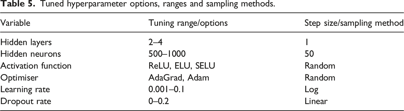
The AdaGrad (Adaptive Sub-gradient Descent) optimiser is provided as an option for training since the dataset features localised effects and wide variations in outputs (Duchi et al., 2011). Additionally, it was proved to work effectively for blast applications of ANNs by Dennis et al. (2021) due to how its variable learning rate results in common features having smaller impacts on the weight and bias updates whilst rare features have larger impacts (Hadgu et al., 2015). Similarly, Zahedi & Golchin (2022) notes that the Adam optimiser tends to perform well for most studies, providing a useful alternative.

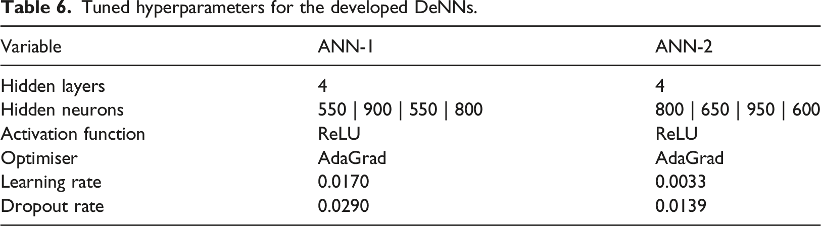
Tuned parameters are provided in Table 6 for ANN-1 and ANN-2.

Table 6.

Tuned hyperparameters for the developed DeNNs.

Variable	ANN-1	ANN-2
Hidden layers	4	4
Hidden neurons	550 \| 900 \| 550 \| 800	800 \| 650 \| 950 \| 600
Activation function	ReLU	ReLU
Optimiser	AdaGrad	AdaGrad
Learning rate	0.0170	0.0033
Dropout rate	0.0290	0.0139

Performance metrics

Comparisons between each network variation will be made using three metrics. The first is the Young’s Correlation Coefficient, calculated using equation (2).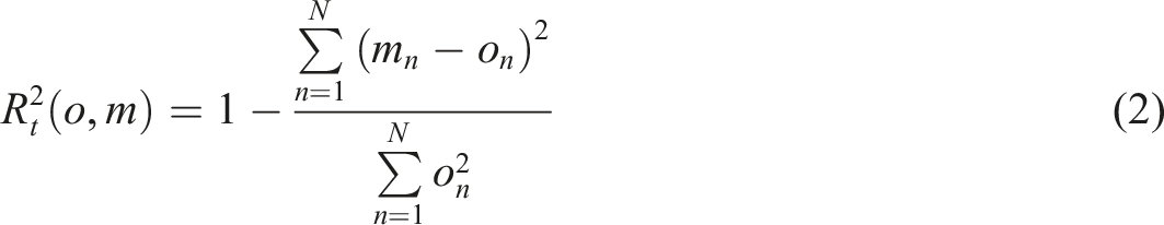

R_{t}^{2} (o, m) = 1 - \frac{\sum_{n = 1}^{N} {(m_{n} - o_{n})}^{2}}{\sum_{n = 1}^{N} o_{n}^{2}}

(2)

where

R_{t}^{2}

is the correlation coefficient, m_n is the predicted peak overpressure, o_n is the target peak overpressure and N is the total number of data points. An

R_{t}^{2}

of 1 shows that every prediction equalled every target, values close to 1 show high correlation between the two variables and close to 0 shows little correlation.

The Mean Absolute Error is also used, calculated using equation (3), to assess the average magnitude of error in the predictions using the associated units of kilo pascals.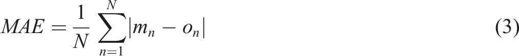

M A E = \frac{1}{N} \sum_{n = 1}^{N} | m_{n} - o_{n} |

(3)

Finally, the average percentage error is calculated using equation (4). This metric removes the influence of magnitude from the error assessments.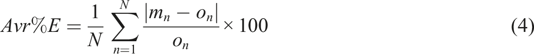

A v r % E = \frac{1}{N} \sum_{n = 1}^{N} \frac{| m_{n} - o_{n} |}{o_{n}} \times 100

(4)

Performance assessment

Training analysis

Mean performance statistics from the 4-fold cross validation technique are reported in Table 7 for the training and validation stages of both ANN-1 and ANN-2. It should be noted that each of the features and development methods detailed in the previous sections were trialled progressively, with improvements in validation performance being observed after each new feature was implemented. For brevity, details of each development stage have been omitted from this article, instead only placing a focus on the features used in the final network.

Table 7.

Mean performance metrics from 4-fold cross validation of the tuned, developed DeNN.

Development stage	ANN number	$R_{t}^{2}$	MAE (kPa)	Average error (%)
Training	1	0.9973	2.63	5.6
Training	2	0.9766	2.38	13.6
Validation	1	0.9967	2.74	5.6
Validation	2	0.9734	2.49	14.0

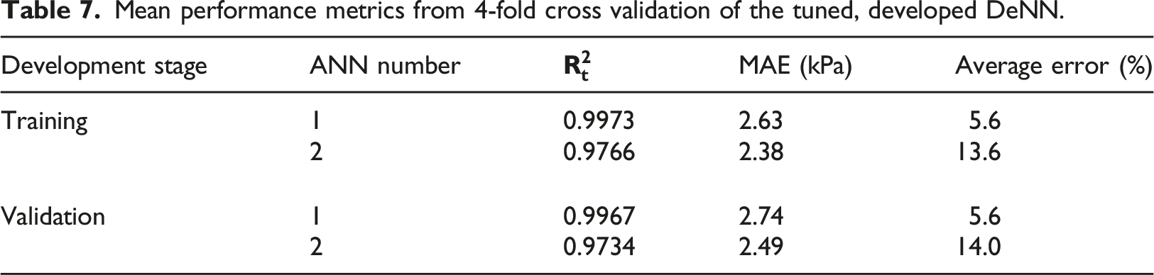
Considering points that are not used to iteratively update the weights and biases, the average error for points that are unobstructed (ANN-1) is 5.6%, corresponding to a MAE of 2.74 kPa. On the other hand, the error of obstructed points (ANN-2) is slightly higher at an average of 14.0%, yet this results in a similar MAE of 2.49 kPa (suggesting a higher propensity for lower magnitude pressure values for this network, as discussed previously). Correlation coefficients of around 0.997 for ANN-1 are comparable to those achieved by Remennikov and Rose (2007) for peak pressure predictions behind blast barriers using a bespoke network structure. However, ANN-2’s correlations around 0.975 suggest that future work should focus on this network’s ability to replicate the relevant wave coalescence effects, especially considering the average errors around 14% are also outside ‘typical’ variations for blast scenarios, being less than 10% (Rigby et al., 2014).

Despite this, there is minimal overfitting as the validation performance is only slightly worse than training in each metric. The dataset is shown to be generalised consistently with different groups of data being held out in four separate training processes.

An assessment of the variation in error from this training and validation process is displayed in Table 8. It shows that lower magnitudes are commonly predicted with higher errors compared to those with larger magnitudes, despite the dataset featuring more points in the lower overpressure ranges. ANN-2, used for predictions of obstructed points, handles a larger number of these lower magnitude targets, hence increasing its average error and decreasing the reported performance.

Table 8.

Variation of tuned network predictive performance during validation relative to the target peak overpressure magnitude.

Target overpressure range (kPa)	Number dataset points	Percentage of validation dataset points predicted within percentage error range (%)
Target overpressure range (kPa)	Number dataset points	E<5	5 ≤ E<10	10 ≤ E<30	E ≥ 30
P < 25	124,128	29.3	21.9	39.0	9.9
25 ≤ P < 50	113,342	51.8	23.5	22.9	1.8
50 ≤ P < 100	75,042	81.3	9.3	8.9	0.4
100 ≤ P < 200	31,090	88.7	7.3	3.7	0.3
200 ≤ P < 300	10,498	86.1	12.1	1.8	0.1
P ≥ 300	454	75.3	15.0	5.5	4.2

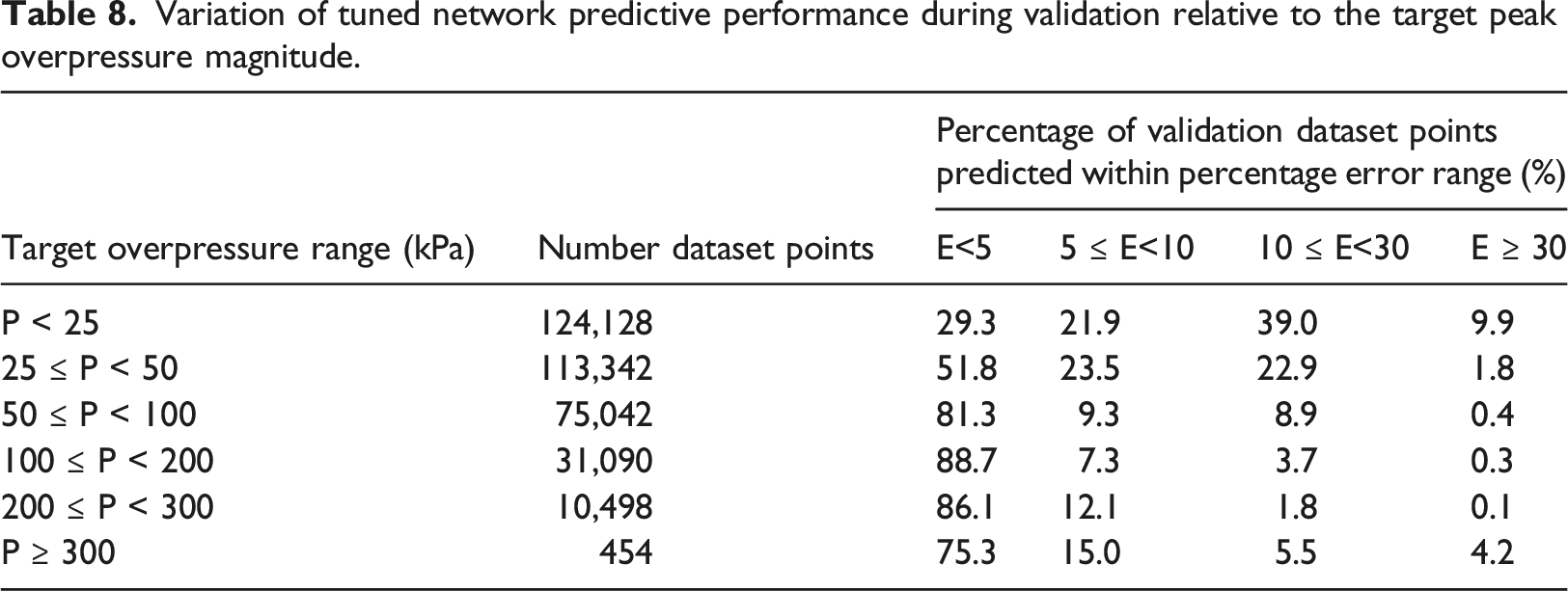
The table also shows how there are only 454 (0.13% of the dataset) targets over 300 kPa, corresponding to around 10% of points having errors over 10% in this overpressure range. The low number of input patterns associated to this range means that the DeNN does not update its weights and biases to suit predictions of this magnitude very often, restricting its ability to accurately account for the needed pressure amplification. However, for points between 50 kPa and 300 kPa, performance is generally very good with average errors of less than 5% for over 81% of the points in each these ranges. Furthermore, over the same targets, less than 0.5% of points are predicted with errors over 30% giving confidence that the DeNN can account for wave interaction effects appropriately.

Testing analysis

Performance metrics obtained when using the tuned and developed DeNN to predict both testing domains are provided in Table 9. There is a decrease in performance compared to the validation and training metrics, yet this is expected considering how the testing models were structured without the same restrictions that were applied to the randomised training dataset.

Table 9.

Performance metrics for both testing domains, simulated using the DeNN, compared to a Viper model.

Testing model	ANN number	$R_{t}^{2}$	MAE (kPa)	Average error (%)
1	1	0.9961	4.18	5.4
	2	0.8989	4.48	42.1
	Overall	0.9952	4.26	16.0
2	1	0.9971	3.90	7.1
	2	0.8070	6.83	57.6
	Overall	0.9938	4.86	23.6

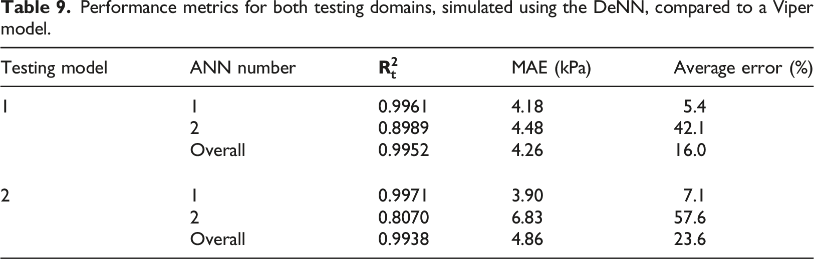
An average MAE around ∼4.5 kPa and correlation coefficients over 0.99 for both domains proves that the DeNN has been able to successfully use its training to generalise for unseen, and independent, inputs. However, average errors throughout both domains are over the 10% target, due to ANN-2 large error contribution of over 40% in both instances. As before, these errors are coupled with low absolute errors suggesting that the points being predicted by this network are of very low magnitude.

Figure 13 presents heat maps for T1, showing the Viper outputs, DeNN predictions and the resulting absolute errors. The wave superposition equation and rotating lasers are proved to work effectively since the DeNN achieves good symmetrical consistency and the magnitude of pressure amplification, caused by wave reflections in front of rigid obstacles, is replicated appropriately across the majority of each surface. As mentioned previously, absolute error is generally very low, aside from the regions where multiple surfaces are close to one another. Here, errors approach 80 kPa in highly localised regions, yet this does not prevent to DeNN from qualitatively representing the distribution of peak overpressure with high accuracy.

Figure 13.

T1 peak overpressure targets generated by Viper::Blast, predictions from the DeNN, and the resulting absolute errors. White regions are not predicted, either due to being within a rigid obstacle, or the 1.5 m exclusion zone.

Conversely, Figure 14, which shows heat maps T2, highlights that channelling is only partially considered. Errors are low where x = 10 and y = 3, but beyond this as x reaches 12, the amplification effects are not as accurate. Additionally, the shape of the high magnitude regions of the DeNN heat maps display some angularity, suggesting that use of 16 lasers contributes to slight local inconsistencies when obstacles are not captured in the input pattern correctly for adjacent points. Despite this, once again, the domain is qualitatively represented by the DeNN with good accuracy, indicating regions where pressure is reduced due to shielding and clearing, whilst amplifying the predictions in front of surfaces.

Figure 14.

T2 peak overpressure targets generated by Viper::Blast, predictions from the DeNN, and the resulting absolute errors. White regions are not predicted, either due to being within a rigid obstacle, or the 1.5 m exclusion zone.

Table 10 shows that the trends within the data are consistent from training to testing when assessing the variation in prediction errors. It is clear that the smaller overpressures are being predicted with the largest percentage errors, but lower absolute errors and that ANN-2 is responsible for the majority of the lower magnitude predictions. Future developments should therefore focus on this network’s ability to handle shielding and clearing effects that can lead to reductions in the peak overpressure when compared to a free air prediction. Targets in the range of 50–200 kPa are once again predicted with good accuracy since the percentage of points with less than 5% error is around 80%, and round 90% are predicted within the desired <10% bracket.

Table 10.

Variation of network predictive performance for both testing models relative to the target peak overpressure magnitude.

Testing models	Target over-pressure range (kPa)	Number dataset points	Percentage of points predicted within percentage error range (%)
Testing models	Target over-pressure range (kPa)	Number dataset points	E<5	5 ≤ E<10	10 ≤ E<30	E ≥ 30
1	P < 25	1560	10.4	9.7	24.7	55.1
	25 ≤ P < 50	1160	40.3	19.4	36.0	4.3
	50 ≤ P < 100	1773	74.3	13.2	11.4	1.0
	100 ≤ P < 200	1136	80.0	10.7	7.8	1.5
	P ≥ 200	310	85.5	14.5	0.0	0.0
2	P < 25	1925	7,7	9.6	19.3	63.4
	25 ≤ P < 50	1407	26.9	16.6	50.6	6.0
	50 ≤ P < 100	1906	77.9	11.4	10.4	0.3
	100 ≤ P < 200	972	88.4	7.1	4.5	0.0
	P ≥ 200	301	87.0	13.0	0.0	0.0

Overall, the achieved performance highlights that physics-informed structuring of the input data provided to ML tools can produce accurate, rapid analysis methods that can be applied to a range of domains. An appreciation for the specific application of the model being developed is essential for understanding how various features of the problem should be represented so that the ANNs can effectively learn from the process and replicate the complex interaction processes.

The next section will explore how this level of performance can be leveraged to allow the DeNN to be used for rapid human injury assessments in its current form.

Prediction of eardrum rupture

To highlight a potential use case for the DeNN, eardrum rupture is predicted according to the rupture levels given by Table 11. This information was compiled by Denny et al. (2021a), and has been used in assessments presented by Denny et al. (2021b, 2022).

Table 11.

Overpressure eardrum rupture limits taken from information presented by Denny et al. (2021a).

Rupture level	Overpressure (kPa)
Threshold	35
50% chance	103
100% chance	202

This criterion is chosen as it relies only on peak overpressure, the only parameter involved in the development of the DeNN so far. It is also the injury criteria that will indicate the regions where other injuries are likely to be experienced, since overpressures below 35 kPa will not cause injury from the blast wave itself.

As shown by Figure 15, the DeNN provides a very good qualitative representation of the various injury zones for T1 when compared to Viper. Only slight variations in output are observed as 95% of points are predicted in the correct rupture category. The remaining 5% are predicted with only one level of error. Regions of shielding are predicted with a ‘no rupture’ designation and transition zones (where clearing occurs) are predicted with a threshold rupture level as the overpressure begins to increase with reduced stand-off distance. The 50% and 100% chance regions are formed in the correct locations, in front of the rigid surfaces and directly around the charge.

Figure 15.

Eardrum rupture levels for T1 calculated by the DeNN and Viper. White regions are not predicted, either due to being within a rigid obstacle, or the 1.5 m exclusion zone.

Rupture predictions for T2 are shown in Figure 16. Here, 93% of points are predicted correctly by the DeNN and the remaining 7% are predicted with only one level of error. The aforementioned issue related to incorrectly amplifying pressure due to channelling as x = 10 and y = 11 is captured in the DeNN’s predictions, and some further inconsistencies are present between the two rigid obstacles to the left of the charge. However, again, the domain is qualitatively well represented.

Figure 16.

Eardrum rupture levels for T2 calculated by the DeNN and Viper. White regions are not predicted, either due to being within a rigid obstacle, or the 1.5 m exclusion zone.

This shows that the DeNN, unlike previous task-specific ML tools, could be used in probabilistic assessments where decisions need to be made rapidly regarding the structural layout of an area, or the regions to focus a response to an explosive event. Its flexibility, achieved using inputs that reference the surrounding and not the domain itself, allows for obstacles to be moved, added or removed, with predictions being generated in under 60 s for an entire domain. Compared to Viper, this allows for upwards of 30 unique layouts to be evaluated in the time that it would take to run a single numerical model from birth to termination.

There are, of course, other applications where the DeNN cannot be used in its current form, and a numerical model should be evaluated using Viper or similar solvers. These include if time varying outputs are required, if non-rectangular or frangible/non-rigid obstacles are present. Conversely, within the current capability of the DeNN, the elevation of the charge and output locations could be repositioned, and the predicted value could be changed to another blast wave parameter that is required by more robust human injury assessments. Although these alterations would require the generation of a new training dataset to train new networks.

Summary and conclusions

In summary, the DeNN is introduced as a novel approach to providing geometrical information to a ML tool, such that it can be used to produce predictions in domains of any shape and size. Unlike previous applications of ANNs in blast engineering that resulted in the development of bespoke tools without this level of generalisation, the DeNN removes the need to encode geometrical information into the network’s architecture when predicting peak overpressure by considering each point’s proximity to surrounding obstacles and the blast wave’s shortest travel distance.

Following a training process using data from 25 randomised domains, it is shown that the DeNN can accurately predict regions of pressure enhancements through reflection and coalescence in addition to shielding and clearing when testing two independent models, with differing structural arrangements. Overpressure distributions throughout both domains were formed in under 60 s, with mean absolute errors less than ∼5 kPa and correlation coefficients above 0.993. Translating this into eardrum rupture levels resulted in over 93% of points being correctly categorised with the remaining percentage only having one level of error.

The inability of other rapid analysis tools to represent complex domain geometries in a general sense limits their application to studies involving only simple geometries and wave interaction effects. Since this is not a limitation of the DeNN it is now feasible to conduct probabilistic assessments, where many domains, featuring various structural layouts, need to be simulated rapidly. Furthermore, the DeNN can be used to generate a prediction for a single point, or a series of points, instead of an entire domain, making it useful for when risk must be assessed at a specific region, such as congregation areas or egress/ingress points.

Since all comparison metrics from training and validation outperformed those obtained throughout testing, the independent testing domains are likely to have provided input patterns that were not common in the training dataset, thus requiring extensive interpolation. Consequently, use of a structured training dataset may improve consistency of predictions with unseen inputs. As probabilistic assessments commonly feature similar domain layouts, data could be taken from the batch to train a new DeNN that could replace the numerical solver part-way through the computation process.

There are still many opportunities for the predictive performance of the DeNN to be improved, however, this article has shown the importance of feature selection in ML models by highlighting that prior knowledge of blast engineering can help to form tools that are more suited to the problems faced in the associated field.

Footnotes

Declaration of conflicting interests

The author(s) declared no potential conflicts of interest with respect to the research, authorship, and/or publication of this article.

Funding

The author(s) disclosed receipt of the following financial support for the research, authorship, and/or publication of this article: Adam A Dennis gratefully acknowledges the financial support from the Engineering and Physical Sciences Research Council (EPSRC) Doctoral Training Partnership.

ORCID iDs

Adam A Dennis

Sam E Rigby

Notes

References

Alterman

Stewart

Netherton

(2019) Probabilistic assessment of airblast variability and fatality risk estimation for explosive blasts in confined building spaces. International Journal of Protective Structures 10(3): 306–329.

Bakalis

Valipour

Bentahar

, et al. (2023) Detonation cell size prediction based on artificial neural networks with chemical kinetics and thermodynamic parameters. Fuel Communications 14(December 2022): 100084.

Bogosian

Yokota

Rigby

(2016) TNT equivalence of C-4 and PE4: a review of traditional sources and recent data. In: Proceedings of the 24th Military Aspects of Blast and Shock, MABS, Halifax, Nova Scotia, Canada, 2016, pp. 19–23.

Chiu

M-C

Yeh

L-J

Lin

(2009) The design and application of a robotic vacuum cleaner. Journal of Information and Optimization Sciences 30(1): 39–62.

Cranz

(1926) Lehrbuch der Basllistik. Berlin, Germany: Springer.

Dennis

Pannell

Smyl

, et al. (2021) Prediction of blast loading in an internal environment using artificial neural networks. International Journal of Protective Structures 12(3): 287–314.

Dennis

Smyl

Stirling

, et al. (2022) A branching algorithm to reduce computational time of batch models: application for blast analyses. International Journal of Protective Structures.

Denny

Langdon

Rigby

, et al. (2022) A numerical investigation of blast-structure interaction effects on primary blast injury risk and the suitability of existing injury prediction methods. International Journal of Protective Structures.

Denny

Dickinson

Langdon

(2021a) Defining blast loading zones of relevance’ for primary blast injury research: a consensus of injury criteria for idealised explosive scenarios. Medical Engineering & Physics 93: 83–92.

10.

Denny

Dickinson

Langdon

(2021b) Guidelines to inform the generation of clinically relevant and realistic blast loading conditions for primary blast injury research. BMJ Military Health.

11.

Duchi

Hazan

Singer

(2011) Adaptive subgradient methods for online learning and stochastic optimization. Journal of Machine Learning Research 12: 2121–2159.

12.

Gallet

Liew

Hajirasouliha

, et al. (2023) Influence Zones of Continuous Beam Systems. Submitted for possible publication in Engineering Structures .

13.

Gan

Brewer

Pope

, et al. (2022) Probabilistic analysis of blast–obstacle interaction in a crowded internal environment. Probabilistic Engineering Mechanics 68: 103227.

14.

Grisaro

Edri

Rigby

(2021) TNT equivalency analysis of specific impulse distribution from close-in detonations. International Journal of Protective Structures 12(3): 315–330.

15.

Hadgu

Nigam

Diaz-Aviles

(2015) Large-scale learning with AdaGrad on Spark. In: 2015 IEEE International Conference on Big Data, Santa Clara, CA, USA, 29 October–1 November 2015, IEEE, 2, pp. 2828–2830.

16.

Hopkinson

(1915) British Ordnance Board Minutes, 13565.

17.

Kang

Park

(2023) Prediction of peak pressure by blast wave propagation between buildings using a conditional 3D convolutional neural network. IEEE Access 11: 26114–26124.

18.

Kang

Kim

Noh

, et al. (2014) A robust obstacle detection method for robotic vacuum cleaners. IEEE Transactions on Consumer Electronics 60(4): 587–595.

19.

Kingery

Bulmash

(1984) Airblast Parameters from TNT Spherical Air Burst and Hemispherical Surface Burst. ARBRL-TR-02555. Maryland, USA: US Army Ballistic Research Laboratory, Aberdeen Proving Ground.

20.

Lee

Hornig

Kury

(1968) Adiabatic Expansion of High Explosive Detonation Products. TID 4500-UCRL 50422., Technical report. CA, USA: University of California.

21.

Jamieson

DeSalvo

, et al. (2018) Hyperband: a novel bandit-based approach to hyperparameter optimization. Journal of Machine Learning Research 18: 1–52.

22.

Wang

, et al. (2023a) Prediction of BLEVE loads on structures using machine learning and CFD. Process Safety and Environmental Protection 171(February): 914–925.

23.

Wang

Shao

, et al. (2023b) A comparative study on the most effective machine learning model for blast loading prediction: from GBDT to Transformer. Engineering Structures 276(December 2022): 115310.

24.

Yan

, et al. (2022) Field test and probabilistic vulnerability assessment of a reinforced concrete bridge pier subjected to blast loads. Engineering Failure Analysis 143(PA): 106802.

25.

Marks

Stewart

Netherton

, et al. (2021) Airblast variability and fatality risks from a VBIED in a complex urban environment. Reliability Engineering & System Safety 209: 107459.

26.

Netherton

Stewart

(2016) Risk-based blast-load modelling: techniques, models and benefits. International Journal of Protective Structures 7(3): 430–451.

27.

O’Malley

Bursztein

Long

, et al. (2019) Kerastuner. https://github.com/keras-team/keras-tuner.

28.

Pannell

Rigby

Panoutsos

(2022a) Application of transfer learning for the prediction of blast impulse. International Journal of Protective Structures.

29.

Pannell

Rigby

Panoutsos

(2022b) Physics-informed regularisation procedure in neural networks: an application in blast protection engineering. International Journal of Protective Structures 13: 555–578.

30.

Pope

(2011) The development of a quick-running prediction tool for the assessment of human injury owing to terrorist attack within crowded metropolitan environments. Philosophical Transactions of the Royal Society of London. Series B, Biological Sciences 366(1562): 127–143.

31.

Rebelo

Cismasiu

(2021) Robustness assessment of a deterministically designed sacrificial cladding for structural protection. Engineering Structures 240(February): 112279.

32.

Remennikov

Gan

ECJ

Tan

, et al. (2022) Methodology for predicting explosion risk around underground coal mine openings towards developing exclusion zones. In: Proceedings of the 2022 Resource Operators Conference, University of Wollongong, 18-20 February 2019, pp. 126–138.

33.

Remennikov

Mendis

(2006) Prediction of airblast loads in complex environments using artificial neural networks. WIT Transactions on the Built Environment 87: 269–278.

34.

Remennikov

Rose

(2007) Predicting the effectiveness of blast wall barriers using neural networks. International Journal of Impact Engineering 34(12): 1907–1923.

35.

Rigby

Gitterman

(2016) Secondary shock delay measurements from explosive trials. In: Proceedings of the 24th Military Aspects of Blast and Shock, Halifax, Nova Scotia, Canada, 2016.

36.

Rigby

Knighton

Clarke

, et al. (2020) Reflected near-field blast pressure measurements using high speed video. Experimental Mechanics 60(7): 875–888.

37.

Rigby

Sielicki

(2014) An investigation of TNT equivalence of hemispherical PE4 charges. Engineering Transactions 62(4): 423–435.

38.

Rigby

Tyas

Fay

, et al. (2014) Validation of semi-empirical blast pressure predictions for far field explosions - is there inherent variability in blast wave parameters? In: 6th International Conference on Protection of Structures Against Hazards, Tianjin, China, October 2014.

39.

Rigby

Fay

Tyas

, et al. (2015) Angle of incidence effects on far-field positive and negative phase blast parameters. International Journal of Protective Structures 6(1): 23–42.

40.

Rose

(2001) An Approach to the Evaluation of Blast Loads on Finite and Semi-infinite Structures. PhD thesis: Engineering Systems Department: Cranfield University.

41.

Seisson

Lacaze

Rouquand

(2020) Uncertainty estimation of external blast effects using the monte-carlo method. WIT Transactions on the Built Environment 198: 81–92.

42.

Wada

Liou

(1997) An accurate and robust flux splitting scheme for shock and contact discontinuities. SIAM Journal on Scientific Computing 18(3): 633–657.

43.

Zaghloul

Remennikov

(2021) Enhancement of blast wave parameters due to shock focusing from multiple simultaneously detonated charges. International Journal of Protective Structures 12(4): 541–576.

44.

Zahedi

Golchin

(2022) Prediction of blast loading on protruded structures using machine learning methods. International Journal of Protective Structures.

The Direction-encoded Neural Network: A machine learning approach to rapidly predict blast loading in obstructed environments

Abstract

Keywords

Introduction

Numerical modelling

Introduction

Mesh sensitivity

Cell size in 3D

Far-field experimental validation

The Direction-encoded Neural Network (DeNN)

Introduction

Input features

Rotating laser directions

Superposition equation

Multiple neural networks

Example input patterns

Dataset development and training

Training dataset

Testing models

Viper::Blast modelling

Network structure

Performance metrics

Performance assessment

Training analysis

Testing analysis

Prediction of eardrum rupture

Summary and conclusions

Footnotes

Declaration of conflicting interests

Funding

ORCID iDs

Notes

References