Three control techniques for suppressing nonlinear vibrations in a 2-DOF dynamical system subjected to combined external and multi-parametric harmonic excitations with 1:1 internal resonance

Abstract

This article addresses the vibration control of a nonlinear two-pole rotor generator system through the application of three distinct control strategies. The equations of motion governing the system are formulated as a nonlinear two-degree-of-freedom model, subjected to a combination of external, linear parametric, and nonlinear parametric excitations. A closed-loop control system is then developed, incorporating the rotor model alongside the proposed control approaches, resulting in six coupled nonlinear differential equations. The proposed control strategies explored are Positive Position Feedback Control ( $PPFC$ ), Integral Resonant Control ( $IRC$ ), and the hybrid approach $PPFC$ + $IRC$ . Utilizing perturbation theory, an accurate analytical solution is derived for the closed-loop system. The bifurcation characteristics of the rotor model are examined, and the vibration reduction effectiveness of the proposed control methods is evaluated. The findings from the analytical investigations reveal that both $PPFC$ and the hybrid $PPFC+IRC$ not only fail to effectively mitigate the vibrations of the rotor under the combined excitations but may also destabilize the system at specific angular velocities. This instability manifests quasi-periodic or unbounded oscillations, which could have potentially destructive consequences. In contrast, the tuned $PPFC+IRC$ combination successfully suppresses the rotor vibrations, reducing them to near zero. However, a loss of tuning conditions in this approach can critically compromise the stability of the closed-loop system. While the $IRC$ strategy is less effective at vibration suppression compared to the tuned $PPFC+IRC$ , it is more robust against instability, simpler, and more reliable, making it the optimal control strategy for such systems. Finally, numerical simulations of all derived analytical results demonstrated the accuracy of the analytical solution despite the complexity of the introduced mathematical model.

Introduction

Nonlinear vibrations frequently occur in rotating machines due to factors like geometric nonlinearities, material properties, cracks, or external excitations. These vibrations can cause instability, accelerated wear, and even system failure, making it crucial to analyze their causes and behavior. Recognizing the contributors to nonlinear vibrations such as rotor imbalance, misalignment, and friction is key to ensuring accurate diagnosis and effective control. For decades, researchers worldwide have focused on identifying the sources of nonlinearities in rotating machinery and analyzing their effects on dynamic behavior. Nearly twenty years ago, Cveticanin ¹ explored the free vibrations of a simple Jeffcott rotor model incorporating cubic nonlinear restoring forces. The author applied the Krylov–Bogolubov technique to assess the rotor’s sensitivity to initial conditions. His findings indicated that the rotor may oscillate in a straight path if started with an initial deflection, while a nonzero initial velocity could result in oscillation along a circular path. Several studies have thoroughly analyzed rotor dynamics, focusing on nonlinear restoring forces and external excitations.^2–5 Adiletta et al. ² explored the impact of adjustable nonlinear stiffness on aperiodic oscillations in rotor models, demonstrating that changes in stiffness and excitation amplitudes could result in quasiperiodic behavior. Ishida and Inoue ³ investigated the internal resonance in a Jeffcott rotor model under gyroscopic effects, revealing complex resonance patterns and nearly periodic oscillations influenced by asymmetrical nonlinearity. Yabuno et al. ⁴ examined a horizontally mounted rotor system with cubic nonlinear restoring forces, reducing it to a 2-DOF model. Their study showed that small frequency differences between horizontal and vertical directions caused localized and nonlocalized vibrations depending on the eccentricity magnitude. Malgol et al. ⁵ later studied the role of hydrodynamic forces and gyroscopic effects on the Yabuno et al. model in Ref. 4, concluding that high-viscosity lubricants significantly dampen system vibrations. In Ref. 6, Malgol et al. investigated the linear continuous rotor model, concentrating on the system parameters that affect rotor resonance frequency. Their findings indicated that the resonance frequency of the rotor system increases with the mass ratio, radius of gyration, and end spring stiffness, while it decreases with the mass moment of inertia of the disc. The internal damping parameter was identified as the primary factor influencing system stability. Han et al. ⁷ examined the impact of an initial shaft bow on the dynamics of a nonlinear rotor, focusing on the interactions between nonlinearities arising from the fluid-film damper and cubic restoring forces. Their findings revealed that the initial shaft bow has a minimal effect on system dynamics for small rotor length-to-diameter ratios, while it significantly influences dynamics in cases of larger rotor length-to-diameter ratios. Lin et al. ⁸ and Chen et al. ⁹ studied the influences of the bearings' nonlinearities on the vibration behavior of both dual-disk and dual-rotor subjected to multi-frequency excitation. They reported that variations in system parameters can result in saddle-node and Hopf bifurcations, along with the emergence of multivalued solutions and symmetry-breaking effects. Saeed et al. ¹⁰ demonstrated the emergence of quasi-periodic and chaotic responses in a nonlinear rotor model with a transverse crack. Ghasabi et al.^11,12 studied the dynamic characteristics of micro-rotating shafts. Key findings reveal that the critical speed, amplitude, and limit cycle radius are significantly influenced by damping coefficients and the material length scale parameter. Increasing the length scale parameter decreases the limit cycle radius while increasing critical speed, with modified couple stress theory results converging toward classical theory as the length scale parameter decreases.

The impact of asymmetric stiffness on rotor dynamics has been thoroughly examined in the literature.^13–18 Whether intentionally introduced or arising from manufacturing defects, asymmetry in rotor stiffness represents a dangerous form of parametric excitation in the mathematical models that describe the dynamics of these systems. ¹³ Srinath et al. and Yi et al.^14–16 carried out a thorough examination of instability within rotor models featuring lumped parameters and continuous asymmetric stiffness. Through the application of Floquet and perturbation theories, they investigated the stability limits related to different system parameters. A key outcome indicates that greater damping leads to a decrease in the unstable parameter range, thereby improving the stability of the shaft’s operational range. Additionally, their findings showed that the flexibility of the bearings creates extra unstable regions, which are less significant in practical applications compared to those associated with rigid bearings. Furthermore, Bavi et al.^17,18 investigated the nonlinear vibrations of a thin-walled rotor with asymmetric stiffness under the influence of either eccentricity or gyroscopic effects.

To improve the stability of rotating machinery and extend its operational lifespan, passive, active, or a combination of both control strategies are employed to reduce the adverse effects of vibrations.^19–22 Passive methods, such as tuned mass dampers and vibration isolators,^23–26 focus on absorbing or redirecting energy, while active strategies like feedback and adaptive control actively counter vibrations by adjusting system parameters in real-time. Implementing active control for rotor vibrations requires specialized actuators with features like fast response, adaptability, contactless operation, and high reliability, where Active Magnetic Bearings (AMB) stand out as ideal candidates. Several configurations of AMB actuators have been investigated, with Ji et al.^27,28 being among the pioneers in examining the bifurcation behavior of four-pole and eight-pole AMB actuators with constant stiffness under $PD-$ controller. In Ref. 29, 30, advanced control strategies, including nonlinear $-PD$ and $PD+IRC$ , were developed to enhance bifurcation control in constant-stiffness eight-pole AMBs. Zhang et al.^31,32 focused on the vibrational dynamics of eight-pole AMBs with time-varying stiffness, revealing their intricate chaotic behavior. Furthermore, studies on sixteen-pole AMBs with both constant and time-varying stiffness determined that constant-stiffness AMBs offer superior dynamic stability.^33,34 AMBs have also been utilized as ideal actuators in various semi-active ³⁵ and active^36–38 control methods to mitigate undesirable rotor vibrations. Time delay is an inherent and unavoidable factor in active control systems.^39,40 Ghasabi et al. investigated the influence of loop delays on the performance of a $PD-$ controller employed to mitigate the resonant vibrations of continuous symmetric ⁴¹ and continuous asymmetric ⁴² rotor models. Their key findings showed that the rotor system may be subjected to Hopf bifurcation because of the existence of loop delays. Additionally, they reported that the stability margin related to loop delays is proportional to both the derivative and proportional control gains. The effect of time delay on the performance of $PPFC$ in controlling the resonant oscillations of both lumped parameter and continuous rotor models was explored by Saeed et al. ⁴³ and Ghasabi et al., ⁴⁴ respectively. The authors reported that although controller performance can be improved by increasing the control and/or feedback gains, the stability margin for loop delays is inversely proportional to both control and feedback gains. Ghasabi et al. ⁴⁵ also explored the performance of time-delayed saturation control in reducing the undesired vibrations of a continuous rotor model. They reported that the negative effects of time delay on closed-loop stability necessitate minimizing the delay as much as possible. Recently, Saeed et al. ⁴⁶ and Elashmawey et al. ⁴⁷ studied the effectiveness of both linear and nonlinear versions of the $IRC$ in mitigating lateral vibrations in a nonlinear rotor model influenced by simultaneous external and multiparametric excitations. Their research concluded that the linear $IRC$ was more effective in suppressing system oscillations compared to its nonlinear counterpart. However, the system’s maximum vibration amplitude was observed at perfect resonance conditions. Various numerical and analytical methods have been extensively employed to investigate nonlinear dynamical systems.^48–50 Among the analytical techniques, the homotopy perturbation method (HPM) and the multiple-scale perturbation method (MSM) stand out as powerful tools for addressing nonlinear oscillations. HPM, along with its subsequent advancements by Prof. He et al.,^51–55 including the variational iteration method and a simplified frequency formulation, integrates traditional perturbation techniques with the concept of homotopy from topology. This approach enables an iterative solution process without requiring small perturbation parameters, making it particularly effective for approximating solutions to a wide range of nonlinear oscillators and differential equations. Conversely, the multiple-scale perturbation method (MSM) ⁵⁶ is a classical perturbation technique that introduces multiple time scales to distinguish between fast and slow dynamics in weakly nonlinear systems. By systematically eliminating secular terms, MSM ensures long-term accuracy in approximate solutions, making it especially useful for analyzing resonance phenomena and amplitude-frequency relationships. This method is particularly advantageous for handling complex nonlinear dynamical systems involving mixed excitation modes and multiple degrees of freedom. While HPM provides a flexible and straightforward approach for solving nonlinear equations in the time domain, MSM excels in capturing intricate modulation effects and resonance behavior in the frequency domain, which aligns with the focus of this study.

In contrast to previous studies on vibration control of asymmetric rotor models subjected to simultaneous external, linear parametric, and nonlinear parametric excitations, Saeed et al. ⁴⁶ and Elashmawey et al. ⁴⁷ analyzed the effectiveness of both linear and nonlinear versions of IRC in mitigating lateral vibrations. Their findings indicated that both control approaches enhanced system damping, reduced nonlinear effects, and eliminated multistable solutions. However, while the linear IRC proved more effective in suppressing oscillations than its nonlinear counterpart, both strategies exhibited peak vibration amplitudes at perfect resonance conditions. Building on this, the present work introduces, for the first time, the PPFC and a combined PPFC + IRC strategy to evaluate their performance against the previously studied IRC approach.^46,47 A comprehensive mathematical model of the closed-loop control system was developed for each strategy, and perturbation methods were employed to analyze the system’s response under the three control configurations: PPFC, IRC, and PPFC + IRC. The derived analytical solutions provided insights into the controllers' ability to stabilize rotor motion and mitigate oscillations. The results reveal that both PPFC and IRC + PPFC, if not properly tuned, fail to effectively suppress vibrations or stabilize the system. However, when optimally tuned, the IRC + PPFC strategy significantly reduces vibrations to near zero, regardless of excitation forces or angular velocity. Nevertheless, improper tuning can critically compromise the stability of the closed-loop system. On the other hand, while the linear IRC strategy is less effective than the tuned IRC + PPFC in vibration suppression, it demonstrates greater robustness against instability, making it a more cost-effective and reliable alternative. Thus, the choice between IRC and IRC + PPFC depends on the desired trade-off between high-performance vibration suppression (offered by the IRC + PPFC, albeit with increased cost and complexity) and a more economical yet stable IRC controller.

Asymmetric two-pole rotor model and control system

Within this section, the mathematical model of the asymmetric two-pole rotor system, equipped with a magnetic actuator and the proposed control system, is developed. The dynamical equations governing the vibrations of the asymmetric two-rotor model, illustrated in Figure 1, are expressed as follows^46,47,57

$m\ddot{x}+c_1\dot{x}+F_x=m\hspace{0.17em}f{\omega }^2\hspace{0.17em}\cos \left(\omega t+\beta \right),$

(1.1)

$m\ddot{y}+c_2\dot{y}+F_y=m\hspace{0.17em}f{\omega }^2\hspace{0.17em}\sin \left(\omega t+\beta \right),$

(1.2)

where $x\left(t\right)$ and $y\left(t\right)$ is the lateral instantaneous displacement of the rotor center $C\left(x\left(t\right),y\left(t\right)\right)$ away from the origin $O$ of the inertial frame $XY$ , $m$ is the mass of the two-pole rotor, $c_1$ and $c_2$ are the linear damping, $f$ denotes the eccentricity, $\omega$ is the angular velocity, and $F_x$ and $F_y$ are the restoring forces in $X$ and $Y$ direction. To find an accurate mathematical model of $F_x$ and $F_y$ , let us assume the rotational reference frame $Z_1{Z}_2$ with angular velocity $\omega$ , where $\overrightarrow{O{Z}_1}$ direction refers to the low-stiffness direction while $\overrightarrow{O{Z}_2}$ direction is the high stiffness direction as shown in (1b). For the small displacements $z_1\left(t\right)$ and $z_2\left(t\right)$ in $\overrightarrow{O{Z}_1}$ and $\overrightarrow{O{Z}_2}$ directions, one can express the restoring forces $F_{Z_1}$ in $\overrightarrow{O{Z}_1}$ and $F_{Z_2}$ in $\overrightarrow{O{Z}_2}$ as follows ⁵⁷

$F_{Z_1}=-\left(k_1-\mathrm{\Delta }{k}_1\right)z_1-\left(k_2-\mathrm{\Delta }{k}_2\right)z_1^3,$

(2.1)

$F_{Z_2}=-\left(k_1+\mathrm{\Delta }{k}_1\right)z_2-\left(k_2+\mathrm{\Delta }{k}_2\right)z_2^3,$

(2.2)

where $k_1$ and $k_2$ are the linear and nonlinear stiffness coefficients of the two poles rotor, while $\mathrm{\Delta }{k}_1$ and $\mathrm{\Delta }{k}_2$ is linear and nonlinear stiffness differences due to the shat asymmetry.

Figure 1.

Asymmetric rotor model: (a) three-dimensional representation of two-pole rotor generator, and (b) schematic diagram of two-pole rotor generator cross-sectional area.

According to the geometry of Figure 1(b), the relation between $x\left(t\right),y\left(t\right),z_1\left(t\right),$ and $z_2\left(t\right)$ can be obtained as follows

$z_1=x\hspace{0.17em}\cos \left(\omega t\right)+y\hspace{0.17em}\sin \left(\omega t\right),$

(3.1)

$z_2=-x\hspace{0.17em}\sin \left(\omega t\right)+y\hspace{0.17em}\cos \left(\omega t\right),$

(3.2)

In addition, the relationship between $F_x,F_y,F_{Z_1},$ and $F_{Z_2}$ can be expressed such that

$F_x=F_{Z_1}\hspace{0.17em}\cos \left(\omega t\right)-F_{Z_2}\hspace{0.17em}\sin \left(\omega t\right),$

(4.1)

$F_y=F_{Z_1}\hspace{0.17em}\sin \left(\omega t\right)+F_{Z_2}\hspace{0.17em}\cos \left(\omega t\right),$

(4.2)

Substituting from equations (2.1)–(4.2) into equations (1.1) and (1.2), yields

$\begin{array}{l}m\ddot{x}+c_1\dot{x}-\left(k_1-\mathrm{\Delta }{k}_1\right)\left[x\hspace{0.17em}{\cos }^2\left(\omega t\right)+y\hspace{0.17em}\cos \left(\omega t\right)\sin \left(\omega t\right)\right]-\left(k_2-\mathrm{\Delta }{k}_2\right)[x^3\hspace{0.17em}{\cos }^4\left(\omega t\right)\\ +3x^{2}y\hspace{0.17em}{\cos }^3\left(\omega t\right)\sin \left(\omega t\right)+3x{y}^2\hspace{0.17em}{\cos }^2\left(\omega t\right){\sin }^2\left(\omega t\right)+y^3\hspace{0.17em}\cos \left(\omega t\right){\sin }^3\left(\omega t\right)]+\left(k_1+\mathrm{\Delta }{k}_1\right)[-x\hspace{0.17em}{\sin }^2\left(\omega t\right)\\ +y\hspace{0.17em}\cos \left(\omega t\right)\sin \left(\omega t\right)]+\left(k_2+\mathrm{\Delta }{k}_2\right)[-x^3\hspace{0.17em}{\sin }^4\left(\omega t\right)+3x^{2}y\hspace{0.17em}\cos \left(\omega t\right){\sin }^3\left(\omega t\right)-3x{y}^2\hspace{0.17em}{\cos }^2\left(\omega t\right){\sin }^2\left(\omega t\right)\\ +y^3\hspace{0.17em}{\cos }^3\left(\omega t\right)\sin \left(\omega t\right)]=m\hspace{0.17em}f{\omega }^2\hspace{0.17em}\cos \left(\omega t+\beta \right)+N_1,\end{array}$

(5.1)

$\begin{array}{l}m\ddot{y}+c_2\dot{y}-\left(k_1-\mathrm{\Delta }{k}_1\right)\left[x\hspace{0.17em}\cos \left(\omega t\right)\sin \left(\omega t\right)+y\hspace{0.17em}{\sin }^2\left(\omega t\right)\right]-\left(k_2-\mathrm{\Delta }{k}_2\right)[x^3\hspace{0.17em}{\cos }^3\left(\omega t\right)\sin \left(\omega t\right)\\ +3x^{2}y\hspace{0.17em}{\cos }^2\left(\omega t\right){\sin }^2\left(\omega t\right)+3x{y}^2\hspace{0.17em}\cos \left(\omega t\right){\sin }^3\left(\omega t\right)+y^3\hspace{0.17em}{\sin }^4\left(\omega t\right)]-\left(k_1+\mathrm{\Delta }{k}_1\right)[-x\hspace{0.17em}\cos \left(\omega t\right)\sin \left(\omega t\right)\\ +y\hspace{0.17em}{\cos }^2\left(\omega t\right))-\left(k_2+\mathrm{\Delta }{k}_2\right)([-x^3\hspace{0.17em}\cos \left(\omega t\right){\sin }^3\left(\omega t\right)+3x^{2}y\hspace{0.17em}{\cos }^2\left(\omega t\right){\sin }^2\left(\omega t\right)-3x{y}^2\hspace{0.17em}{\cos }^3\left(\omega t\right)\sin \left(\omega t\right)\\ +y^3\hspace{0.17em}{\cos }^4\left(\omega t\right)]=m\hspace{0.17em}f{\omega }^2\hspace{0.17em}\sin \left(\omega t+\beta \right)+N_2,\end{array}$

(5.2)

where $N_1$ and $N_2$ represent the net control forces proposed to be applied in $X$ and $Y$ directions, respectively, via a magnetic actuator as electromagnetic attraction forces, according to the proposed control technique to eliminate the rotor undesired oscillations. To mitigate the undesired lateral displacements $x\left(t\right)$ and $y\left(t\right)$ of the considered two-pole rotor model, three different control techniques have been introduced within the work utilizing four pole magnetic bearings as an actuator as shown in Figure 2. The physical interconnection between the rotor and the control system via two displacement sensors and a four-pole actuator has been illustrated in Figure 2(a), where the four poles produce the four forces $F_1,F_2,F_3$ , and $F_4$ that form a push-pull control mechanism to counteract the undesired oscillation of the rotor system $x\left(t\right)$ and $y\left(t\right)$ . The magnitudes of the electromagnetic forces $F_1,F_2,F_3$ , and $F_4$ are functions of the electrical currents flow in the electromagnetic poles as well as the airgap size between the rotor and the poles, accordingly the net control forces $N_1$ and $N_2$ in $X$ and $Y$ directions can be expressed as follows ⁵⁸

$N_1=F_1-F_2=\Phi \left[{\left(\frac{I_b-I_x}{h-x}\right)}^2-{\left(\frac{I_b+I_x}{h+x}\right)}^2\right],$

(6.1)

$N_2=F_3-F_4=\Phi \left[{\left(\frac{I_b-I_y}{h-y}\right)}^2-{\left(\frac{I_b+I_y}{h+y}\right)}^2\right],$

(6.2)

where $\mathit{\Phi }$ is an electromagnetic coupling constant, $h$ is the nominal airgap between the rotor and the poles, $I_b$ is constant current defined as bias current to energize the electrical coils, and $I_x$ and $I_y$ are the control current in $X$ and $Y$ directions.

Figure 2.

Asymmetric two-pole rotor model equipped with active controller and magnetic actuator: (a) Physical interconnections between rotor, controller, and actuator; and (b) control strategy flow chart.

The $PPFC,IRC,$ and the combination of both (i.e., $PPFC+IRC$ ) have been investigated for undesired vibration control of the system considered. Accordingly, the control currents $I_x$ and $I_y$ can be expressed as follows ⁵⁹

$I_x=-\left[k_{11}{u}_1\left(t\right)+k_{12}{v}_1\left(t\right)\right],$

(7.1)

$I_y=-\left[k_{21}{u}_2\left(t\right)+k_{22}{v}_2\left(t\right)\right],$

(7.2)

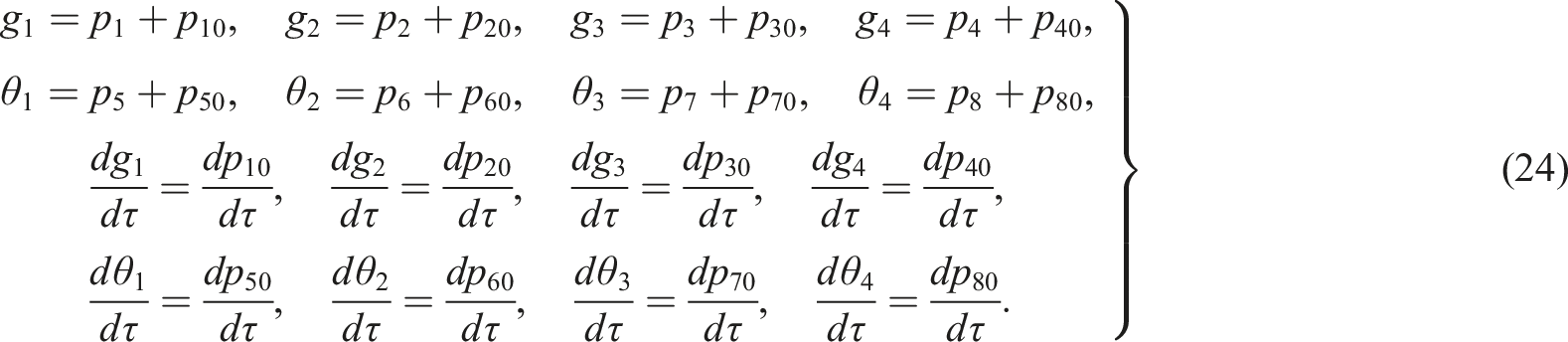
where $k_{11}{u}_1\left(t\right)$ and $k_{21}{u}_2\left(t\right)$ are control action of the $PPFC$ , while $k_{12}{v}_1\left(t\right)$ and $k_{22}{v}_2\left(t\right)$ denote the control action of the $IRC$ . The differential equations governing the dynamics of both the $PPFC$ and $IRC$ are given as follows

${\ddot{u}}_1+k_{31}{\dot{u}}_1+k_{32}{u}_1=k_{33}x,$

(8.1)

${\ddot{u}}_2+k_{41}{\dot{u}}_2+k_{42}{u}_2=k_{43}y,$

(8.2)

${\dot{v}}_1+k_{51}{v}_1=k_{52}x,$

(8.3)

${\dot{v}}_2+k_{61}{v}_2=k_{62}y.$

(8.4)

By inserting equations (7.1) and (7.2) into equations (6.1) and (6.2), then expanding the resulting equations utilizing the Maclaurin series up to the third-order approximation, yield

$\begin{array}{l}{N}_1=\frac{4\mathrm{\Phi }}{h^4}[h^3{I}_b{k}_{11}{u}_1+h^3{I}_b{k}_{12}{v}_1+h^2{I}_b^{2}x+2I_b^2{x}^3+3h{I}_b{k}_{11}{u}_1{x}^2+3h{I}_b{k}_{12}{v}_1{x}^2+h^2{k}_{11}^{2}x{u}_1^2\\ +2h^2{k}_{11}{k}_{12}{u}_1{v}_{1}x+h^2{k}_{12}^2{v}_1^{2}x],\end{array}$

(9.1)

$\begin{array}{l}{N}_2=\frac{4\mathrm{\Phi }}{h^4}[h^3{I}_b{k}_{21}{u}_2+h^3{I}_b{k}_{22}{v}_2+h^2{I}_b^{2}y+2I_b^2{y}^3+3h{I}_b{k}_{21}{u}_2{y}^2+3h{I}_b{k}_{22}{v}_2{y}^2+h^2{k}_{21}^{2}y{u}_2^2\\ +2h^2{k}_{21}{k}_{22}{u}_2{v}_{2}y+h^2{k}_{22}^2{v}_2^{2}y].\end{array}$

(9.2)

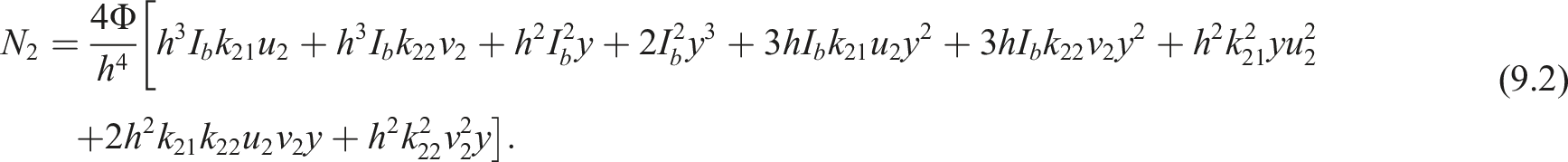
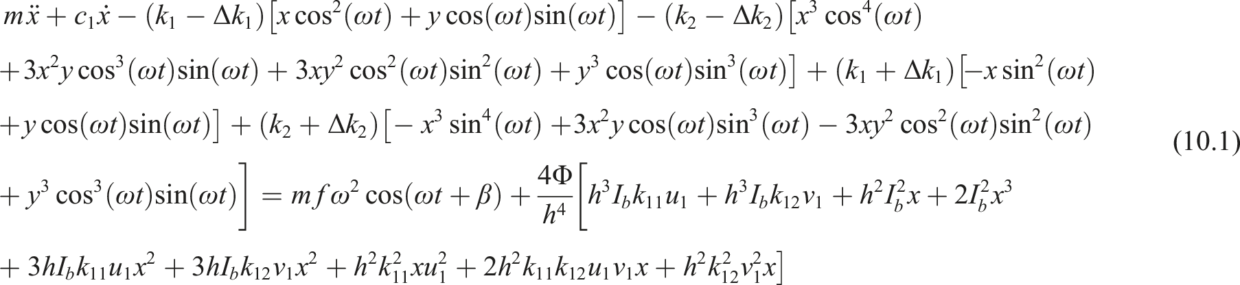
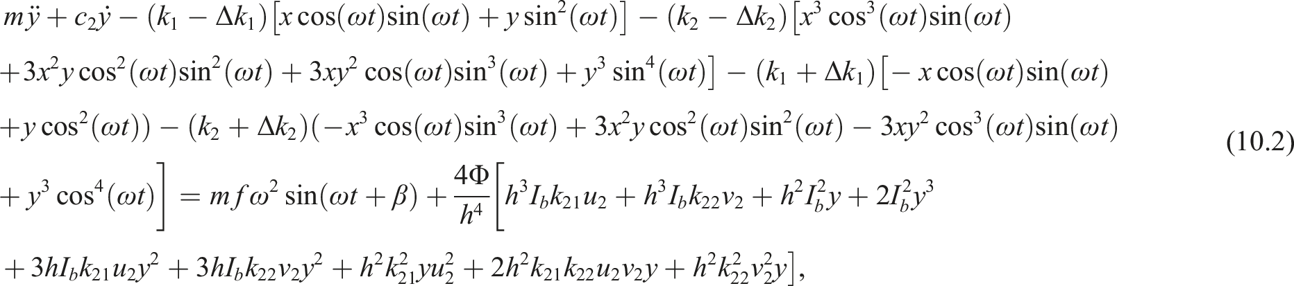
Substituting equations (9.1) and (9.2) into equations (5.1) and (5.2), we have from equations (5.1), (5.2), (8.1), (8.2), (8.3), and (8.4) the following closed-loop control system

$\begin{array}{l}m\ddot{x}+c_1\dot{x}-\left(k_1-\mathrm{\Delta }{k}_1\right)\left[x\hspace{0.17em}{\cos }^2\left(\omega t\right)+y\hspace{0.17em}\cos \left(\omega t\right)\sin \left(\omega t\right)\right]-\left(k_2-\mathrm{\Delta }{k}_2\right)[x^3\hspace{0.17em}{\cos }^4\left(\omega t\right)\\ +3x^{2}y\hspace{0.17em}{\cos }^3\left(\omega t\right)\sin \left(\omega t\right)+3x{y}^2\hspace{0.17em}{\cos }^2\left(\omega t\right){\sin }^2\left(\omega t\right)+y^3\hspace{0.17em}\cos \left(\omega t\right){\sin }^3\left(\omega t\right)]+\left(k_1+\mathrm{\Delta }{k}_1\right)[-x\hspace{0.17em}{\sin }^2\left(\omega t\right)\\ +y\hspace{0.17em}\cos \left(\omega t\right)\sin \left(\omega t\right)]+\left(k_2+\mathrm{\Delta }{k}_2\right)[-x^3\hspace{0.17em}{\sin }^4\left(\omega t\right)+3x^{2}y\hspace{0.17em}\cos \left(\omega t\right){\sin }^3\left(\omega t\right)-3x{y}^2\hspace{0.17em}{\cos }^2\left(\omega t\right){\sin }^2\left(\omega t\right)\\ +y^3\hspace{0.17em}{\cos }^3\left(\omega t\right)\sin \left(\omega t\right)]=m\hspace{0.17em}f{\omega }^2\hspace{0.17em}\cos \left(\omega t+\beta \right)+\frac{4\mathrm{\Phi }}{h^4}[h^3{I}_b{k}_{11}{u}_1+h^3{I}_b{k}_{12}{v}_1+h^2{I}_b^{2}x+2I_b^2{x}^3\\ +3h{I}_b{k}_{11}{u}_1{x}^2+3h{I}_b{k}_{12}{v}_1{x}^2+h^2{k}_{11}^{2}x{u}_1^2+2h^2{k}_{11}{k}_{12}{u}_1{v}_{1}x+h^2{k}_{12}^2{v}_1^{2}x]\end{array}$

(10.1)

$\begin{array}{l}m\ddot{y}+c_2\dot{y}-\left(k_1-\mathrm{\Delta }{k}_1\right)\left[x\hspace{0.17em}\cos \left(\omega t\right)\sin \left(\omega t\right)+y\hspace{0.17em}{\sin }^2\left(\omega t\right)\right]-\left(k_2-\mathrm{\Delta }{k}_2\right)[x^3\hspace{0.17em}{\cos }^3\left(\omega t\right)\sin \left(\omega t\right)\\ +3x^{2}y\hspace{0.17em}{\cos }^2\left(\omega t\right){\sin }^2\left(\omega t\right)+3x{y}^2\hspace{0.17em}\cos \left(\omega t\right){\sin }^3\left(\omega t\right)+y^3\hspace{0.17em}{\sin }^4\left(\omega t\right)]-\left(k_1+\mathrm{\Delta }{k}_1\right)[-x\hspace{0.17em}\cos \left(\omega t\right)\sin \left(\omega t\right)\\ +y\hspace{0.17em}{\cos }^2\left(\omega t\right))-\left(k_2+\mathrm{\Delta }{k}_2\right)(-x^3\hspace{0.17em}\cos \left(\omega t\right){\sin }^3\left(\omega t\right)+3x^{2}y\hspace{0.17em}{\cos }^2\left(\omega t\right){\sin }^2\left(\omega t\right)-3x{y}^2\hspace{0.17em}{\cos }^3\left(\omega t\right)\sin \left(\omega t\right)\\ +y^3\hspace{0.17em}{\cos }^4\left(\omega t\right)]=m\hspace{0.17em}f{\omega }^2\hspace{0.17em}\sin \left(\omega t+\beta \right)+\frac{4\mathrm{\Phi }}{h^4}[h^3{I}_b{k}_{21}{u}_2+h^3{I}_b{k}_{22}{v}_2+h^2{I}_b^{2}y+2I_b^2{y}^3\\ +3h{I}_b{k}_{21}{u}_2{y}^2+3h{I}_b{k}_{22}{v}_2{y}^2+h^2{k}_{21}^{2}y{u}_2^2+2h^2{k}_{21}{k}_{22}{u}_2{v}_{2}y+h^2{k}_{22}^2{v}_2^{2}y],\end{array}$

(10.2)

${\ddot{u}}_1+k_{31}{\dot{u}}_1+k_{32}{u}_1=k_{33}x,$

(10.3)

${\ddot{u}}_2+k_{41}{\dot{u}}_2+k_{42}{u}_2=k_{43}y,$

(10.4)

${\dot{v}}_1+k_{51}{v}_1=k_{52}x,$

(10.5)

${\dot{v}}_2+k_{61}{v}_2=k_{62}y.$

(10.6)

The engineering implementation of the proposed control process is illustrated in detail in Figure 2(b), where the figure shows the signals flow chart between the rotor and the controllers (i.e., $PPFC$ and $IRC$ ).

Dimensionless equations of motion, approximate solution, and stability analysis

Normalized equations of motion

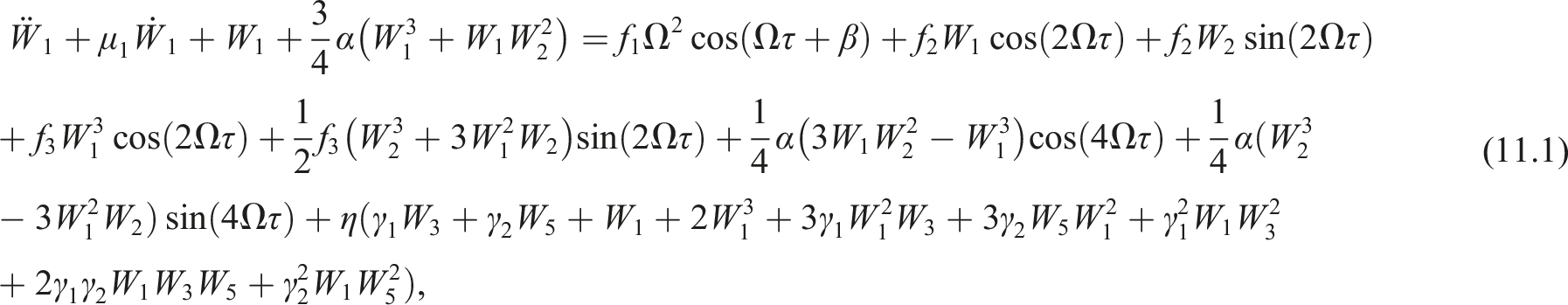
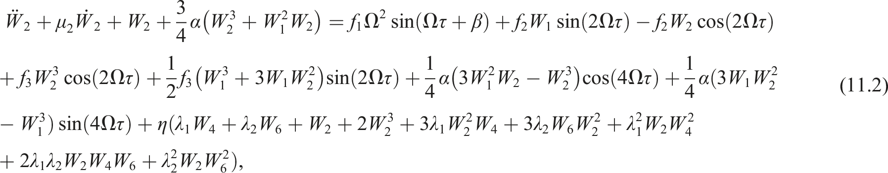
To generalize the derived mathematical model presented in equations (10.1)–(10.6), the system is nondimensionalized using the following dimensionless variables: $W_1=x/h,W_2=y/h,W_3=u_1/h,W_4=u_2/h,W_5=v_1/h$ , $W_6=v_2/h$ , $\tau ={\omega }_{n}t$ , where ${\omega }_n=\sqrt{k_1/m}$ represents the rotor’s natural frequency. Here, $W_1$ represents the relative dimensionless instantaneous oscillation of the rotor in the $X-$ direction, normalized by the air-gap size ( $h$ ) between the rotor and stator, while $W_2$ denotes the relative instantaneous oscillation of the rotor in the $Y-$ direction, also normalized by the air-gap size. The resulting dimensionless dynamical system is given as follows

$\begin{array}{l}{\ddot{W}}_1+{\mu }_1{\dot{W}}_1+W_1+\frac{3}{4}\alpha \left(W_1^3+W_1{W}_2^2\right)=f_1{\mathrm{\Omega }}^2\hspace{0.17em}\cos \left(\mathrm{\Omega }\tau +\beta \right)+f_2{W}_1\hspace{0.17em}\cos \left(2\mathrm{\Omega }\tau \right)+f_2{W}_2\hspace{0.17em}\sin \left(2\mathrm{\Omega }\tau \right)\\ +f_3{W}_1^3\hspace{0.17em}\cos \left(2\mathrm{\Omega }\tau \right)+\frac{1}{2}{f}_3\left(W_2^3+3W_1^2{W}_2\right)\sin \left(2\mathrm{\Omega }\tau \right)+\frac{1}{4}\alpha \left(3W_1{W}_2^2-W_1^3\right)\cos \left(4\mathrm{\Omega }\tau \right)+\frac{1}{4}\alpha (W_2^3\\ -3W_1^2{W}_2)\hspace{0.17em}\sin \left(4\mathrm{\Omega }\tau \right)+\eta ({\gamma }_1{W}_3+{\gamma }_2{W}_5+W_1+2W_1^3+3{\gamma }_1{W}_1^2{W}_3+3{\gamma }_2{W}_5{W}_1^2+{\gamma }_1^2{W}_1{W}_3^2\\ +2{\gamma }_1{\gamma }_2{W}_1{W}_3{W}_5+{\gamma }_2^2{W}_1{W}_5^2),\end{array}$

(11.1)

$\begin{array}{l}{\ddot{W}}_2+{\mu }_2{\dot{W}}_2+W_2+\frac{3}{4}\alpha \left(W_2^3+W_1^2{W}_2\right)=f_1{\mathrm{\Omega }}^2\hspace{0.17em}\sin \left(\mathrm{\Omega }\tau +\beta \right)+f_2{W}_1\hspace{0.17em}\sin \left(2\mathrm{\Omega }\tau \right)-f_2{W}_2\hspace{0.17em}\cos \left(2\mathrm{\Omega }\tau \right)\\ +f_3{W}_2^3\hspace{0.17em}\cos \left(2\mathrm{\Omega }\tau \right)+\frac{1}{2}{f}_3\left(W_1^3+3W_1{W}_2^2\right)\sin \left(2\mathrm{\Omega }\tau \right)+\frac{1}{4}\alpha \left(3W_1^2{W}_2-W_2^3\right)\cos \left(4\mathrm{\Omega }\tau \right)+\frac{1}{4}\alpha (3W_1{W}_2^2\\ -W_1^3)\hspace{0.17em}\sin \left(4\mathrm{\Omega }\tau \right)+\eta ({\lambda }_1{W}_4+{\lambda }_2{W}_6+W_2+2W_2^3+3{\lambda }_1{W}_2^2{W}_4+3{\lambda }_2{W}_6{W}_2^2+{\lambda }_1^2{W}_2{W}_4^2\\ +2{\lambda }_1{\lambda }_2{W}_2{W}_4{W}_6+{\lambda }_2^2{W}_2{W}_6^2),\end{array}$

(11.2)

${\ddot{W}}_3+{\mu }_3{\dot{W}}_3+{\omega }_1^2{W}_3={\zeta }_1{W}_1,$

(11.3)

${\ddot{W}}_4+{\mu }_4{\dot{W}}_4+{\omega }_2^2{W}_4={\zeta }_2{W}_2,$

(11.4)

${\dot{W}}_5+{\rho }_1{W}_5={\delta }_1{W}_1,$

(11.5)

${\dot{W}}_6+{\rho }_2{W}_6={\delta }_2{W}_2,$

(11.6)

where ${\mu }_1=c_1/\sqrt{k_{1}m},{\mu }_2=c_2/\sqrt{k_{1}m},{\mu }_3=k_{31}/\sqrt{k_{1}m},{\mu }_4=k_{41}/\sqrt{k_{1}m},\alpha =h^2{k}_2/k_1,f_1=f/h,f_2=\mathit{\Delta }{k}_1/k_1,f_3=h^2\mathit{\Delta }{k}_2/k_1,{\gamma }_1=h{k}_{11}/I_b,{\gamma }_2=h{k}_{12}/I_b,{\lambda }_1=h{k}_{21}/I_b,{\lambda }_2=h{k}_{22}/I_b,{\rho }_1=k_{51}/\sqrt{k_1/m},{\rho }_2=k_{61}/\sqrt{k_1/m},{\delta }_1=k_{52}/\sqrt{k_1/m},{\delta }_2=k_{62}/\sqrt{k_1/m},\eta =4\mathrm{\Phi }{I}_b^2/h{k}_1,{\zeta }_1=mh{k}_{33}/k_1,{\hspace{0.17em}\zeta }_2=mh{k}_{43}/k_1,{\omega }_1=\sqrt{m{k}_{32}/k_1},{\omega }_2=\sqrt{m{k}_{42}/k_1}$ , and $\mathrm{\Omega }=\frac{\omega }{{\omega }_n}$ . Accordingly, the variables $W_1\left(\tau \right)$ and $W_2\left(\tau \right)$ represent the dimensionless instantaneous vibration of the two-pole rotor model in $X$ and $Y$ directions, $W_3\left(\tau \right)$ and $W_4\left(\tau \right)$ denote the instantaneous displacement of the $PPFC$ , and $W_5\left(\tau \right)$ and $W_6\left(\tau \right)$ are the dimensionless displacements of the $IRC$ . In addition, ${\gamma }_1$ and ${\lambda }_1$ are the dimensionless control gain of the $PPFC$ , while ${\gamma }_2$ and ${\lambda }_2$ denote the control gains of the $IRC$ . To evaluate the efficiency of the $PPFC$ , $IRC$ , and $PPFC+IRC$ in suppressing the unwanted vibrations of the considered two-pole rotor model analytical solutions for the complicated control system model given by equations (11.1) to (11.6) is as given in the following section.

Multiple time-scale perturbation solution

Based on the complexity of the derived dimensionless mathematical model, the multiple time-scales perturbation technique ( $MSPT$ ) is applied to obtain an analytical solution for equations (11.1)–(11.6). Accordingly, let’s assume the solution of equations (11.1)–(11.6) as follows ⁵⁶

$W_n\left(\tau ,\epsilon \right)=W_{n0}\left(T_0,T_1\right)+\epsilon W_{n1}\left(T_0,T_1\right),n=1,2,3,4$

(12.1)

$W_n\left(\tau ,\epsilon \right)=\epsilon W_{n0}\left(T_0,T_1\right)+{\epsilon }^2{W}_{n1}\left(T_0,T_1\right),n=5,6,$

(12.2)

where $\epsilon$ is a book-keeping perturbation parameter, ${\hspace{0.17em}T}_0=\tau ,$ and ${\hspace{0.17em}T}_1=\epsilon \tau$ . In terms of ${\hspace{0.17em}T}_0$ and ${\hspace{0.17em}T}_1$ , the derivatives $\frac{d}{d\tau }$ and $\frac{d^2}{{d\tau }^2}$ can be expressed such that

$\frac{d}{d\tau }=D_0+\epsilon D_1,\frac{d^2}{d{\tau }^2}=D_0^2+2\epsilon D_0{D}_1,D_j=\frac{\partial }{\partial T_j},j=0,1$

(13)

$\begin{array}{l}{\mu }_1=\epsilon {\widehat{\mu }}_1,{\mu }_2=\epsilon {\widehat{\mu }}_2,{\mu }_3=\epsilon {\widehat{\mu }}_3,{\mu }_4=\epsilon {\widehat{\mu }}_4,\alpha =\epsilon \widehat{\alpha },\eta =\epsilon \widehat{\eta },{\gamma }_2={\epsilon }^{-1}{\widehat{\gamma }}_2,{\lambda }_2={\epsilon }^{-1}{\widehat{\lambda }}_2,\\ {\zeta }_1=\epsilon {\widehat{\zeta }}_1,{\zeta }_2=\epsilon {\widehat{\zeta }}_2,{\delta }_1=\epsilon {\widehat{\delta }}_1,{\delta }_2=\epsilon {\widehat{\delta }}_2,f_1=\epsilon {\widehat{f}}_1,f_2=\epsilon {\widehat{f}}_2,{\widehat{f}}_3=\epsilon {\widehat{f}}_3.\end{array}\}$

(14)

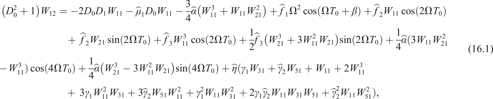
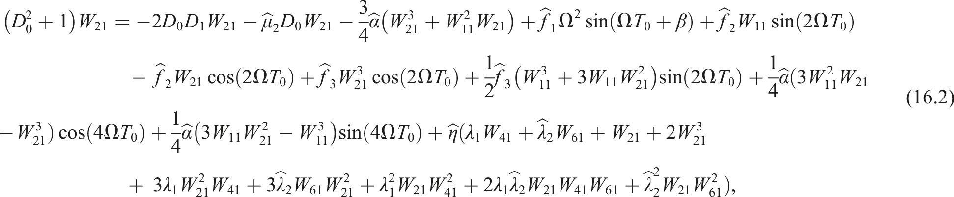
Inserting equations (12.1)–(14) into equations (11.1)–(11.6), then applying the multiple time-scales solution procedure, we have

O ( ${\mathrm{\epsilon }}^0$ )

$\left(D_0^2+1\right)W_{11}=0,$

(15.1)

$\left(D_0^2+1\right)W_{21}=0,$

(15.2)

$\left(D_0^2+{\omega }_1^2\right)W_{31}=0,$

(15.3)

$\left(D_0^2+{\omega }_2^2\right)W_{41}=0,$

(15.4)

O ( ${\mathrm{\epsilon }}^1$ )

$\begin{array}{l}\left(D_0^2+1\right)W_{12}=-2D_0{D}_1{W}_{11}-{\widehat{\mu }}_1{D}_0{W}_{11}-\frac{3}{4}\widehat{\alpha }\left(W_{11}^3+W_{11}{W}_{21}^2\right)+{\widehat{f}}_1{\mathrm{\Omega }}^2\hspace{0.17em}\cos \left(\mathrm{\Omega }{T}_0+\beta \right)+{\widehat{f}}_2{W}_{11}\hspace{0.17em}\cos \left(2\mathrm{\Omega }{T}_0\right)\\ +{\widehat{f}}_2{W}_{21}\hspace{0.17em}\sin \left(2\mathrm{\Omega }{T}_0\right)+{\widehat{f}}_3{W}_{11}^3\hspace{0.17em}\cos \left(2\mathrm{\Omega }{T}_0\right)+\frac{1}{2}{\widehat{f}}_3\left(W_{21}^3+3W_{11}^2{W}_{21}\right)\sin \left(2\mathrm{\Omega }{T}_0\right)+\frac{1}{4}\widehat{\alpha }(3W_{11}{W}_{21}^2\\ -W_{11}^3)\hspace{0.17em}\cos \left(4\mathrm{\Omega }{T}_0\right)+\frac{1}{4}\widehat{\alpha }\left(W_{21}^3-3W_{11}^2{W}_{21}\right)\sin \left(4\mathrm{\Omega }{T}_0\right)+\widehat{\eta }({\gamma }_1{W}_{31}+{\widehat{\gamma }}_2{W}_{51}+W_{11}+2W_{11}^3\\ +3{\gamma }_1{W}_{11}^2{W}_{31}+3{\widehat{\gamma }}_2{W}_{51}{W}_{11}^2+{\gamma }_1^2{W}_{11}{W}_{31}^2+2{\gamma }_1{\widehat{\gamma }}_2{W}_{11}{W}_{31}{W}_{51}+{\widehat{\gamma }}_2^2{W}_{11}{W}_{51}^2),\end{array}$

(16.1)

$\begin{array}{l}\left(D_0^2+1\right)W_{21}=-2D_0{D}_1{W}_{21}-{\widehat{\mu }}_2{D}_0{W}_{21}-\frac{3}{4}\widehat{\alpha }\left(W_{21}^3+W_{11}^2{W}_{21}\right)+{\widehat{f}}_1{\mathrm{\Omega }}^2\hspace{0.17em}\sin \left(\mathrm{\Omega }{T}_0+\beta \right)+{\widehat{f}}_2{W}_{11}\hspace{0.17em}\sin \left(2\mathrm{\Omega }{T}_0\right)\\ -{\widehat{f}}_2{W}_{21}\hspace{0.17em}\cos \left(2\mathrm{\Omega }{T}_0\right)+{\widehat{f}}_3{W}_{21}^3\hspace{0.17em}\cos \left(2\mathrm{\Omega }{T}_0\right)+\frac{1}{2}{\widehat{f}}_3\left(W_{11}^3+3W_{11}{W}_{21}^2\right)\sin \left(2\mathrm{\Omega }{T}_0\right)+\frac{1}{4}\widehat{\alpha }(3W_{11}^2{W}_{21}\\ -W_{21}^3)\hspace{0.17em}\cos \left(4\mathrm{\Omega }{T}_0\right)+\frac{1}{4}\widehat{\alpha }\left(3W_{11}{W}_{21}^2-W_{11}^3\right)\sin \left(4\mathrm{\Omega }{T}_0\right)+\widehat{\eta }({\lambda }_1{W}_{41}+{\widehat{\lambda }}_2{W}_{61}+W_{21}+2W_{21}^3\\ +3{\lambda }_1{W}_{21}^2{W}_{41}+3{\widehat{\lambda }}_2{W}_{61}{W}_{21}^2+{\lambda }_1^2{W}_{21}{W}_{41}^2+2{\lambda }_1{\widehat{\lambda }}_2{W}_{21}{W}_{41}{W}_{61}+{\widehat{\lambda }}_2^2{W}_{21}{W}_{61}^2),\end{array}$

(16.2)

$\left(D_0^2+{\omega }_1^2\right)W_{32}=-2D_0{D}_1{W}_{31}-{\widehat{\mu }}_3{\dot{W}}_{31}+{\widehat{\zeta }}_1{W}_{11},$

(16.3)

$\left(D_0^2+{\omega }_2^2\right)W_{42}=-2D_0{D}_1{W}_{41}-{\widehat{\mu }}_4{\dot{W}}_{41}+{\widehat{\zeta }}_2{W}_{21},$

(16.4)

$\left(D_0+{\rho }_1\right)W_{51}={\widehat{\delta }}_1{W}_{11},$

(16.5)

$\left(D_0+{\rho }_2\right)W_{61}={\widehat{\delta }}_2{W}_{21}.$

(16.6)

The solution of Equations (15.1)–(15.4), (16.5), and (16.6) can be as follows

$W_{11}\left(T_0,T_1\right)=A\left(T_1\right)e^{i{T}_0}+\overline{A}\left(T_1\right)e^{-i{T}_0},$

(17.1)

$W_{21}\left(T_0,T_1\right)=B\left(T_1\right)e^{i{T}_0}+\overline{B}\left(T_1\right)e^{-i{T}_0},$

(17.2)

$W_{31}\left(T_0,T_1\right)=C\left(T_1\right)e^{i{\omega }_1{T}_0}+\overline{C}\left(T_1\right)e^{-i{\omega }_1{T}_0},$

(17.3)

$W_{41}\left(T_0,T_1\right)=D\left(T_1\right)e^{i{\omega }_2{T}_0}+\overline{D}\left(T_1\right)e^{-i{\omega }_2{T}_0},$

(17.4)

$W_{51}\left(T_0,T_1\right)=\frac{\left({\rho }_1-i\right)}{\left({\rho }_1^2+1\right)}{\widehat{\delta }}_{1}A\left(T_1\right)e^{i{T}_0}+\frac{\left({\rho }_1+i\right)}{\left({\rho }_1^2+1\right)}{\widehat{\delta }}_1\overline{A}\left(T_1\right)e^{-i{T}_0},$

(17.5)

$W_{61}\left(T_0,T_1\right)=\frac{\left({\rho }_2-i\right)}{\left({\rho }_2^2+1\right)}{\widehat{\delta }}_{2}B\left(T_1\right)e^{i{T}_0}+\frac{\left({\rho }_2+i\right)}{\left({\rho }_2^2+1\right)}{\widehat{\delta }}_2\overline{B}\left(T_1\right)e^{-i{T}_0},$

(17.6)

where $i=\sqrt{-1}$ , $A\left(T_1\right)$ , $B\left(T_1\right)$ , $C\left(T_1\right)$ and $D\left(T_1\right)$ are unknown to be defined later. $\overline{A},$ $\overline{B}$ , $\overline{C}$ , and $\overline{D}$ are the conjugate of $A$ , $B$ , $C,$ and $D$ , respectively. To extract the solvability condition, let the parameters ${\sigma }_1$ , ${\sigma }_2$ and ${\hspace{0.17em}\sigma }_3$ describe the closeness of the rotational speed ( $\mathrm{\Omega }$ ) as well as $PPFC$ natural frequencies ( ${\omega }_1,{\omega }_2$ ) to the two-pole rotor model normalized natural frequency as follows

$\Omega =1+{\sigma }_1=1+\epsilon {\widehat{\sigma }}_1,{\omega }_1=1+{\sigma }_2=1+\epsilon {\widehat{\sigma }}_2,{\omega }_2=1+{\sigma }_3=1+\epsilon {\widehat{\sigma }}_3.$

(18)

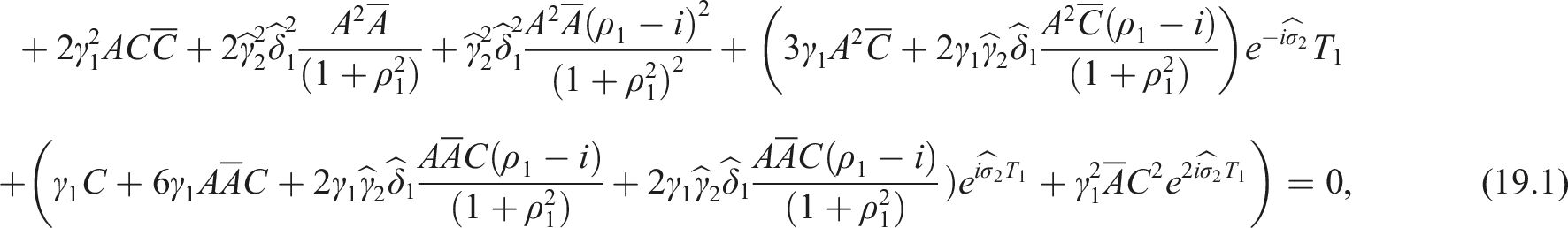
Now, inserting equations (17.1)–(18) into equations (16.1) to (16.4) one can obtain the solvability conditions as follows

$-2i{D}_{1}A-i{\widehat{\mu }}_{1}A-\frac{9}{4}\widehat{\alpha }{A}^2\overline{A}-\frac{3}{2}\widehat{\alpha }AB\overline{B}-\frac{3}{4}\widehat{\alpha }\overline{A}{B}^2+\frac{1}{2}{\widehat{f}}_1{\Omega }^2{e}^{i\left({\widehat{\sigma }}_1{T}_1+\beta \right)}+\frac{1}{2}{\widehat{f}}_2\overline{A}{e}^{2i{\widehat{\sigma }}_1{T}_1}-\frac{i}{2}{\widehat{f}}_2\overline{B}{e}^{2i{\widehat{\sigma }}_1{T}_1}$

$+\frac{3}{2}{\widehat{f}}_{3}A{\overline{A}}^2{e}^{2i{\widehat{\sigma }}_1{T}_1}+\frac{1}{2}{\widehat{f}}_3{A}^3{e}^{-2i{\widehat{\sigma }}_1{T}_1}-\frac{3i}{4}{\widehat{f}}_{3}B{\overline{B}}^2{e}^{2i{\widehat{\sigma }}_1{T}_1}+\frac{i}{4}{\widehat{f}}_3{B}^3{e}^{-2i{\widehat{\sigma }}_1{T}_1}-\frac{3i}{4}{\widehat{f}}_3{\overline{A}}^{2}B{e}^{2i{\widehat{\sigma }}_1{T}_1}$

$+\frac{3i}{4}{\widehat{f}}_3{A}^{2}B{e}^{-2i{\widehat{\sigma }}_1{T}_1}-\frac{3i}{2}{\widehat{f}}_{3}A\overline{A}\overline{B}{e}^{2i{\widehat{\sigma }}_1{T}_1}+\frac{3}{8}\widehat{\alpha }\overline{A}{\overline{B}}^2{e}^{4i{\widehat{\sigma }}_1{T}_1}-\frac{1}{8}\widehat{\alpha }{\overline{A}}^3{e}^{4i{\widehat{\sigma }}_1{T}_1}-\frac{i}{8}\widehat{\alpha }{\overline{B}}^3{e}^{4i{\widehat{\sigma }}_1{T}_1}$

$+\frac{3i}{8}\widehat{\alpha }\overline{B}{\overline{A}}^2{e}^{4i{\widehat{\sigma }}_1{T}_1}+\widehat{\eta }({\widehat{\gamma }}_2{\widehat{\delta }}_1\frac{A\left({\rho }_1-i\right)}{\left(1+{\rho }_1^2\right)}+A+6A^2\overline{A}+3{\widehat{\gamma }}_2{\widehat{\delta }}_1\frac{A^2\overline{A}\left({\rho }_1+i\right)}{\left(1+{\rho }_1^2\right)}+6{\widehat{\gamma }}_2{\widehat{\delta }}_1\frac{A^2\overline{A}\left({\rho }_1-i\right)}{\left(1+{\rho }_1^2\right)}$

$+2{\gamma }_1^{2}AC\overline{C}+2{\widehat{\gamma }}_2^2{\widehat{\delta }}_1^2\frac{A^2\overline{A}}{\left(1+{\rho }_1^2\right)}+{\widehat{\gamma }}_2^2{\widehat{\delta }}_1^2\frac{A^2\overline{A}{\left({\rho }_1-i\right)}^2}{{\left(1+{\rho }_1^2\right)}^2}+\left(3{\gamma }_1{A}^2\overline{C}+2{\gamma }_1{\widehat{\gamma }}_2{\widehat{\delta }}_1\frac{A^2\overline{C}\left({\rho }_1-i\right)}{\left(1+{\rho }_1^2\right)}\right)e^{-i{\widehat{\sigma }}_2{T}_1}+\left({\gamma }_{1}C+6{\gamma }_{1}A\overline{A}C+2{\gamma }_1{\widehat{\gamma }}_2{\widehat{\delta }}_1\frac{A\overline{A}C\left({\rho }_1-i\right)}{\left(1+{\rho }_1^2\right)}+2{\gamma }_1{\widehat{\gamma }}_2{\widehat{\delta }}_1\frac{A\overline{A}C\left({\rho }_1-i\right)}{\left(1+{\rho }_1^2\right)})e^{i{\widehat{\sigma }}_2{T}_1}+{\gamma }_1^2\overline{A}{C}^2{e}^{2i{\widehat{\sigma }}_2{T}_1}\right)=0,$

(19.1)

$-2i{D}_{1}B-i{\widehat{\mu }}_{2}B-\frac{9}{4}\widehat{\alpha }{B}^2\overline{B}-\frac{3}{2}\widehat{\alpha }A\overline{A}B-\frac{3}{4}\widehat{\alpha }\overline{B}{A}^2-\frac{i}{2}{\widehat{f}}_1{\Omega }^2{e}^{i\left({\widehat{\sigma }}_1{T}_1+\beta \right)}-\frac{i}{2}{\widehat{f}}_2\overline{A}{e}^{2i{\widehat{\sigma }}_1{T}_1}-\frac{1}{2}{\widehat{f}}_2\overline{B}{e}^{2i{\widehat{\sigma }}_1{T}_1}$

$+\frac{3}{2}{\widehat{f}}_{3}B{\overline{B}}^2{e}^{2i{\widehat{\sigma }}_1{T}_1}+\frac{1}{2}{\widehat{f}}_3{B}^3{e}^{-2i{\widehat{\sigma }}_1{T}_1}-\frac{3i}{4}{\widehat{f}}_{3}A{\overline{A}}^2{e}^{2i{\widehat{\sigma }}_1{T}_1}+\frac{i}{4}{\widehat{f}}_3{A}^3{e}^{-2i{\widehat{\sigma }}_1{T}_1}-\frac{3i}{4}{\widehat{f}}_3{\overline{B}}^{2}A{e}^{2i{\widehat{\sigma }}_1{T}_1}$

$+\frac{3i}{4}{\widehat{f}}_3{B}^{2}A{e}^{-2i{\widehat{\sigma }}_1{T}_1}-\frac{3i}{2}{\widehat{f}}_{3}B\overline{B}\overline{A}{e}^{2i{\widehat{\sigma }}_1{T}_1}+\frac{3}{8}\widehat{\alpha }\overline{B}{\overline{A}}^2{e}^{4i{\widehat{\sigma }}_1{T}_1}-\frac{1}{8}\widehat{\alpha }{\overline{B}}^3{e}^{4i{\widehat{\sigma }}_1{T}_1}+\frac{i}{8}\widehat{\alpha }{\overline{A}}^3{e}^{4i{\widehat{\sigma }}_1{T}_1}$

$-\frac{3i}{8}\widehat{\alpha }\overline{A}{\overline{B}}^2{e}^{4i\left(\Omega -1\right)\tau }+\widehat{\eta }({\widehat{\lambda }}_2{\widehat{\delta }}_2\frac{B\left({\rho }_2-i\right)}{\left(1+{\rho }_2^2\right)}+B+6B^2\overline{B}+3{\widehat{\lambda }}_2{\widehat{\delta }}_2\frac{B^2\overline{B}\left({\rho }_2+i\right)}{\left(1+{\rho }_2^2\right)}+6{\widehat{\lambda }}_2{\widehat{\delta }}_2\frac{B^2\overline{B}\left({\rho }_2-i\right)}{\left(1+{\rho }_2^2\right)}$

$+2{\lambda }_1^{2}BD\overline{D}+2{\widehat{\lambda }}_2^2{\widehat{\delta }}_2^2\frac{B^2\overline{B}}{\left(1+{\rho }_2^2\right)}+{\widehat{\lambda }}_2^2{\widehat{\delta }}_2^2\frac{B^2\overline{B}{\left({\rho }_2-i\right)}^2}{{\left(1+{\rho }_2^2\right)}^2}+\left(3{\lambda }_1{B}^2\overline{D}+2{\lambda }_1{\widehat{\lambda }}_2{\widehat{\delta }}_2\frac{B^2\overline{D}\left({\rho }_2-i\right)}{\left(1+{\rho }_2^2\right)}\right)e^{-i{\widehat{\sigma }}_3{T}_1}+\left({\lambda }_{1}D+6{\lambda }_{1}B\overline{B}D+2{\lambda }_1{\widehat{\lambda }}_2{\widehat{\delta }}_2\frac{B\overline{B}D\left({\rho }_2+i\right)}{\left(1+{\rho }_2^2\right)}+2{\lambda }_1{\widehat{\lambda }}_2{\widehat{\delta }}_2\frac{B\overline{B}D\left({\rho }_2-i\right)}{\left(1+{\rho }_2^2\right)})e^{i{\widehat{\sigma }}_3{T}_1}+{\lambda }_1^2\overline{B}{D}^2{e}^{2i{\widehat{\sigma }}_3{T}_1}\right)=0,$

(19.2)

$-2i{\omega }_1{D}_{1}C-i{\widehat{\mu }}_3{\omega }_{1}C+{\widehat{\zeta }}_{1}A{e}^{-i{\widehat{\sigma }}_2{T}_0}=0,$

(19.3)

$-2i{\omega }_2{D}_{1}D-i{\widehat{\mu }}_4{\omega }_{2}D+{\widehat{\zeta }}_{2}B{e}^{-i{\stackrel{̑}{\sigma }}_3{T}_0}=0.$

(19.4)

To extract the amplitude-phase equations of the considered closed-loop system, one can express the functions $A\left(T_1\right)$ , $B\left(T_1\right)$ , $C\left(T_1\right)$ and $D\left(T_1\right)$ in the polar form such that ⁵⁶

$A\left(T_1\right)=\frac{1}{2}{g}_1\left(T_1\right)e^{i{\phi }_1\left(T_1\right)},B\left(T_1\right)=\frac{1}{2}{g}_2\left(T_1\right)e^{i{\phi }_2\left(T_1\right)},C\left(T_1\right)=\frac{1}{2}{g}_3\left(T_1\right)e^{i{\phi }_3\left(T_1\right)},D\left(T_1\right)=\frac{1}{2}{g}_4\left(T_1\right)e^{i{\phi }_4\left(T_1\right)}.$

(20)

Inserting equation (20) into equations (19.1)–(19.4) with restoring the scaled parameters in equation (14) to the original form, yield the autonomous dynamical system

$\begin{array}{l}\frac{d{g}_1}{d\tau }=(-\frac{{\mu }_1}{2}-\frac{3\alpha }{32}{g}_2^2\hspace{0.17em}\sin (2{\theta }_2-2{\theta }_1)-\frac{f_2}{4}\sin (2{\theta }_1)-\frac{3\alpha }{64}{g}_2^2\hspace{0.17em}\sin (2{\theta }_2+2{\theta }_1))g_1-(\frac{f_3}{8}\sin (2{\theta }_1)\\ -\frac{\alpha }{64}\sin (4{\theta }_1))g_1^3-\frac{f_2}{4}{g}_2\hspace{0.17em}\cos ({\theta }_2+{\theta }_1)+(-\frac{3f_3}{32}\cos ({\theta }_2+{\theta }_1)+\frac{f_3}{32}\cos (3{\theta }_2-{\theta }_1)\\ -\frac{\alpha }{64}\cos ({\theta }_1+3{\theta }_2))g_2^3-(\frac{3f_3}{32}\cos ({\theta }_2-3{\theta }_1)+\frac{3f_3}{32}\cos ({\theta }_2+{\theta }_1)-\frac{3\alpha }{64}\cos ({\theta }_2+3{\theta }_1))g_1^2{g}_2\\ +\eta (-\frac{1}{2}{\gamma }_2{\delta }_1\frac{g_1}{(1+{\rho }_1^2)}+\frac{3}{8}{\gamma }_2{\delta }_1\frac{g_1^3}{(1+{\rho }_1^2)}-\frac{3}{4}{\gamma }_2{\delta }_1\frac{g_1^3}{(1+{\rho }_1^2)}-\frac{1}{4}{\gamma }_2^2{\delta }_1^2\frac{g_1^3{\rho }_1}{{(1+{\rho }_1^2)}^2}\\ +\frac{1}{8}{\gamma }_1^2{g}_1{g}_3^2\hspace{0.17em}\sin (2{\theta }_3-2{\theta }_1)+(\frac{1}{2}{\gamma }_1{g}_3+\frac{3}{4}{\gamma }_1{g}_1^2{g}_3+\frac{1}{4}{\gamma }_1{\gamma }_2{\delta }_1\frac{g_1^2{g}_3{\rho }_1}{(1+{\rho }_1^2)}+\frac{1}{4}{\gamma }_1{\gamma }_2{\delta }_1\frac{g_1^2{g}_3{\rho }_1}{(1+{\rho }_1^2)})\sin ({\theta }_3-{\theta }_1)\\ +(\frac{3}{8}{\gamma }_1{g}_1^2{g}_3+\frac{1}{4}{\gamma }_1{\gamma }_2{\delta }_1\frac{g_1^2{g}_3{\rho }_1}{(1+{\rho }_1^2)})\sin ({\theta }_1-{\theta }_3)+(-\frac{1}{4}{\gamma }_1{\gamma }_2{\delta }_1\frac{g_1^2{g}_3}{(1+{\rho }_1^2)})\cos ({\theta }_1-{\theta }_3))+\frac{f_1{\mathrm{\Omega }}^2}{2}\sin (\beta -{\theta }_1),\end{array}$

(21.1)

$\begin{array}{l}\frac{d{g}_2}{d\tau }=\left(-\frac{{\mu }_2}{2}-\frac{3\alpha }{32}{g}_1^2\hspace{0.17em}\sin \left(2{\theta }_1-2{\theta }_2\right)+\frac{f_2}{4}\sin \left(2{\theta }_2\right)-\frac{3\alpha }{64}{g}_1^2\hspace{0.17em}\sin \left(2{\theta }_2+2{\theta }_1\right)\right)g_2-(\frac{f_3}{8}\sin \left(2{\theta }_2\right)\\ -\frac{\alpha }{64}\sin \left(4{\theta }_2\right))g_2^3-\frac{f_2}{4}{g}_1\hspace{0.17em}\cos \left({\theta }_2+{\theta }_1\right)+(-\frac{3f_3}{32}\cos \left({\theta }_2+{\theta }_1\right)+\frac{f_3}{32}\cos \left(3{\theta }_1-{\theta }_2\right)\\ +\frac{\alpha }{64}\cos \left({\theta }_2+3{\theta }_1\right))g_1^3-\left(\frac{3f_3}{32}\cos \left({\theta }_1-3{\theta }_2\right)+\frac{3f_3}{32}\cos \left({\theta }_2+{\theta }_1\right)+\frac{3\alpha }{64}\cos \left({\theta }_1+3{\theta }_2\right)\right)g_1{g}_2^2\\ +\eta (-\frac{1}{2}{\lambda }_2{\delta }_2\frac{g_2}{\left(1+{\rho }_2^2\right)}+\frac{3}{8}{\lambda }_2{\delta }_2\frac{g_2^3}{\left(1+{\rho }_2^2\right)}-\frac{3}{4}{\lambda }_2{\delta }_2\frac{g_2^3}{\left(1+{\rho }_2^2\right)}-\frac{1}{4}{\lambda }_2^2{\delta }_2^2\frac{g_2^3{\rho }_2}{{\left(1+{\rho }_2^2\right)}^2}\\ +\frac{1}{8}{\lambda }_1^2{g}_2{g}_4^2\hspace{0.17em}\sin \left(2{\theta }_4-2{\theta }_2\right)+\left(\frac{1}{2}{\lambda }_1{g}_4+\frac{3}{4}{\lambda }_1{g}_2^2{g}_4+\frac{1}{4}{\lambda }_1{\lambda }_2{\delta }_2\frac{g_2^2{g}_4{\rho }_2}{\left(1+{\rho }_2^2\right)}+\frac{1}{4}{\lambda }_1{\lambda }_2{\delta }_2\frac{g_2^2{g}_4{\rho }_2}{\left(1+{\rho }_2^2\right)}\right)\sin \left({\theta }_4-{\theta }_2\right)\\ +\left(\frac{3}{8}{\lambda }_1{g}_2^2{g}_4+\frac{1}{4}{\lambda }_1{\lambda }_2{\delta }_2\frac{g_2^2{g}_4{\rho }_2}{\left(1+{\rho }_2^2\right)}\right)\sin \left({\theta }_2-{\theta }_4\right)+\left(-\frac{1}{4}{\lambda }_1{\lambda }_2{\delta }_2\frac{g_2^2{g}_4}{\left(1+{\rho }_2^2\right)}\right)\cos \left({\theta }_2-{\theta }_4\right))-\frac{f_1{\mathrm{\Omega }}^2}{2}\cos \left(\beta -{\theta }_2\right),\end{array}$

(21.2)

$\frac{d{g}_3}{d\tau }=\frac{-1}{2}{g}_3{\mu }_3+\frac{1}{2}\frac{g_1{\zeta }_1}{{\omega }_1}\sin \left({\theta }_1-{\theta }_3\right),$

(21.3)

$\frac{d{g}_4}{d\tau }=\frac{-1}{2}{g}_4{\mu }_4+\frac{1}{2}\frac{g_2{\zeta }_2}{{\omega }_2}\sin \left({\theta }_2-{\theta }_4\right),$

(21.4)

$\begin{array}{l}\frac{d{\theta }_1}{d\tau }=-{\sigma }_1+\left(\frac{9\alpha }{32}-\frac{f_3}{4}\cos \left(2{\theta }_1\right)+\frac{\alpha }{64}\cos \left(4{\theta }_1\right)\right)g_1^2+(\frac{3\alpha }{32}\cos \left(2{\theta }_2-2{\theta }_1\right)-\frac{3\alpha }{64}\cos \left(2{\theta }_2+2{\theta }_1\right)\\ +\frac{3\alpha }{16})g_2^2-\frac{f_2}{4}\cos \left(2{\theta }_1\right)+\frac{f_2}{4g_1}{g}_2\hspace{0.17em}\sin \left({\theta }_2+{\theta }_1\right)+(\frac{3f_3}{32g_1}\sin \left({\theta }_2+{\theta }_1\right)+\frac{f_3}{32g_1}\sin \left(3{\theta }_2-{\theta }_1\right)\\ +\frac{\alpha }{64g_1}\sin \left({\theta }_1+3{\theta }_2\right))g_2^3-\left(\frac{3f_3}{32}\sin \left({\theta }_2-3{\theta }_1\right)-\frac{9f_3}{32}\sin \left({\theta }_2+{\theta }_1\right)+\frac{3\alpha }{64}\sin \left({\theta }_2+3{\theta }_1\right)\right)g_1{g}_2\\ -\eta (\frac{1}{2}{\gamma }_2{\delta }_1\frac{{\rho }_1}{\left(1+{\rho }_1^2\right)}+\frac{1}{2}+\frac{3}{4}{g}_1^2+\frac{3}{8}{\gamma }_2{\delta }_1\frac{g_1^2{\rho }_1}{\left(1+{\rho }_1^2\right)}+\frac{3}{4}{\gamma }_2{\delta }_1\frac{g_1^2{\rho }_1}{\left(1+{\rho }_1^2\right)}+\frac{1}{4}{\gamma }_1^2{g}_3^2+\frac{1}{4}{\gamma }_2^2{\delta }_1^2\frac{g_1^2}{\left(1+{\rho }_1^2\right)}\\ +\frac{1}{8}{\gamma }_2^2{\delta }_1^2\frac{g_1^2\left({\rho }_1^2-1\right)}{{\left(1+{\rho }_1^2\right)}^2}+\frac{1}{8}{\gamma }_1^2{g}_3^2\hspace{0.17em}\cos \left(2{\theta }_3-2{\theta }_1\right)+(\frac{1}{2}{\gamma }_1\frac{g_3}{g_1}+\frac{3}{4}{\gamma }_1{g}_1{g}_3+\frac{1}{2}{\gamma }_1{\gamma }_2{\delta }_1\frac{g_1{g}_3{\rho }_1}{\left(1+{\rho }_1^2\right)})\cos \left({\theta }_3-{\theta }_1\right)\\ +(\frac{3}{8}{\gamma }_1{g}_1{g}_3+\frac{1}{4}{\gamma }_1{\gamma }_2{\delta }_1\frac{g_1{g}_3{\rho }_1}{\left(1+{\rho }_1^2\right)})\cos \left({\theta }_1-{\theta }_3\right)+\frac{1}{4}{\gamma }_1{\gamma }_2{\delta }_1\frac{g_1{g}_3}{\left(1+{\rho }_1^2\right)}\sin \left({\theta }_1-{\theta }_3\right)(-\frac{f_1{\mathrm{\Omega }}^2}{2g_1}\cos \left(\beta -{\theta }_1\right),\end{array}$

(21.5)

$\begin{array}{l}\frac{d{\theta }_2}{d\tau }=-{\sigma }_1+\left(\frac{9\alpha }{32}-\frac{f_3}{4}\cos \left(2{\theta }_2\right)+\frac{\alpha }{64}\cos \left(4{\theta }_2\right)\right)g_2^2+(\frac{3\alpha }{32}\cos \left(2{\theta }_1-2{\theta }_2\right)-\frac{3\alpha }{64}\cos \left(2{\theta }_2+2{\theta }_1\right)\\ +\frac{3\alpha }{16})g_1^2+\frac{f_2}{4g_2}{g}_1\hspace{0.17em}\sin \left({\theta }_2+{\theta }_1\right)+\frac{f_2}{4}\cos \left(2{\theta }_2\right)+(\frac{3f_3}{32g_2}\sin \left({\theta }_2+{\theta }_1\right)+\frac{f_3}{32g_2}\sin \left(3{\theta }_1-{\theta }_2\right)\\ -\frac{\alpha }{64g_2}\sin \left(3{\theta }_1+{\theta }_2\right))g_1^3-\left(\frac{3f_3}{32}\sin \left({\theta }_1-3{\theta }_2\right)-\frac{9f_3}{32}\sin \left({\theta }_2+{\theta }_1\right)-\frac{3\alpha }{64}\sin \left({\theta }_1+3{\theta }_2\right)\right)g_2{g}_1\\ -\eta (\frac{1}{2}{\lambda }_2{\delta }_2\frac{{\rho }_2}{\left(1+{\rho }_2^2\right)}+\frac{1}{2}+\frac{3}{4}{g}_2^2+\frac{3}{8}{\lambda }_2{\delta }_2\frac{g_2^2{\rho }_2}{\left(1+{\rho }_2^2\right)}+\frac{3}{4}{\lambda }_2{\delta }_2\frac{g_2^2{\rho }_2}{\left(1+{\rho }_2^2\right)}+\frac{1}{4}{\lambda }_1^2{g}_4^2+\frac{1}{4}{\lambda }_2^2{\delta }_2^2\frac{g_2^2}{\left(1+{\rho }_2^2\right)}\\ +\frac{1}{8}{\lambda }_2^2{\delta }_2^2\frac{g_2^2\left({\rho }_2^2-1\right)}{{\left(1+{\rho }_2^2\right)}^2}+\frac{1}{8}{\lambda }_1^2{g}_4^2\hspace{0.17em}\cos \left(2{\theta }_4-2{\theta }_2\right)+(\frac{1}{2}{\lambda }_1\frac{g_4}{g_2}+\frac{3}{4}{\lambda }_1{g}_2{g}_4+\frac{1}{2}{\lambda }_1{\lambda }_2{\delta }_2\frac{g_2{g}_4{\rho }_2}{\left(1+{\rho }_2^2\right)})\cos \left({\theta }_4-{\theta }_2\right)\\ +(\frac{3}{8}{\lambda }_1{g}_2{g}_4+\frac{1}{4}{\lambda }_1{\lambda }_2{\delta }_2\frac{g_2{g}_4{\rho }_2}{\left(1+{\rho }_2^2\right)})\cos \left({\theta }_2-{\theta }_4\right)+\frac{1}{4}{\lambda }_1{\lambda }_2{\delta }_2\frac{g_2{g}_4}{\left(1+{\rho }_2^2\right)}\sin \left({\theta }_2-{\theta }_4\right))-\frac{f_1{\mathrm{\Omega }}^2}{2g_2}\sin \left(\beta -{\theta }_2\right),\end{array}$

(21.6)

$\frac{d{\theta }_3}{d\tau }={\sigma }_2-{\sigma }_1-\frac{1}{2}\frac{{\zeta }_1{g}_1}{g_3{\omega }_1}\cos \left({\theta }_1-{\theta }_3\right),$

(21.7)

$\frac{d{\theta }_4}{d\tau }={\sigma }_3-{\sigma }_1-\frac{1}{2}\frac{{\zeta }_2{g}_2}{g_4{\omega }_2}\cos \left({\theta }_2-{\theta }_4\right),$

(21.8)

where ${\theta }_1={\phi }_1-\mathit{\Omega }\tau +\tau$ , ${\theta }_2={\phi }_2-\mathit{\Omega }\tau +\tau$ , ${\theta }_3={\phi }_3-\mathit{\Omega }\tau +\tau +{\sigma }_2\tau$ , and ${\theta }_4={\phi }_4-\mathit{\Omega }\tau +\tau +{\sigma }_3\tau$ . Substituting Equations (17.1)–(17.6), (18), and (20) into equations (12.1) and (12.2), yield the periodic solution of the closed-loop control system given by Equations (11.1)–(11.6) as follows

$W_1\left(\tau \right)=g_1\left(\tau \right)\cos \left(\mathrm{\Omega }\tau -{\theta }_1\left(\tau \right)\right),$

(22.1)

$W_2\left(\tau \right)=g_2\left(\tau \right)\cos \left(\mathrm{\Omega }\tau -{\theta }_2\left(\tau \right)\right),$

(22.2)

$W_3\left(\tau \right)=g_3\left(\tau \right)\cos \left(\mathrm{\Omega }\tau -\left({\theta }_1\left(\tau \right)+{\theta }_3\left(\tau \right)\right)\right),$

(22.3)

$W_4\left(\tau \right)=g_4\left(\tau \right)\cos \left(\mathrm{\Omega }\tau -\left({\theta }_2\left(\tau \right)+{\theta }_4\left(\tau \right)\right)\right),$

(22.4)

$W_5\left(\tau \right)=\frac{{\delta }_1{g}_1\left(\tau \right)}{\sqrt{{\rho }_1^2+1}}\left[{\rho }_1\hspace{0.17em}\cos \left(\mathrm{\Omega }\tau -{\theta }_1\left(\tau \right)\right)+\sin \left(\mathrm{\Omega }\tau -{\theta }_1\left(\tau \right)\right)\right]=g_5\left(\tau \right)\sin \left(\mathrm{\Omega }\tau -{\theta }_5\left(\tau \right)\right),$

(22.5)

$W_6\left(\tau \right)=\frac{{\delta }_2{g}_2\left(\tau \right)}{\sqrt{{\rho }_2^2+1}}\left[{\rho }_2\hspace{0.17em}\cos \left(\mathrm{\Omega }\tau -{\theta }_2\left(\tau \right)\right)+\sin \left(\mathrm{\Omega }\tau -{\theta }_2\left(\tau \right)\right)\right]=g_6\left(\tau \right)\sin \left(\mathrm{\Omega }\tau -{\theta }_6\left(\tau \right)\right),$

(22.6)

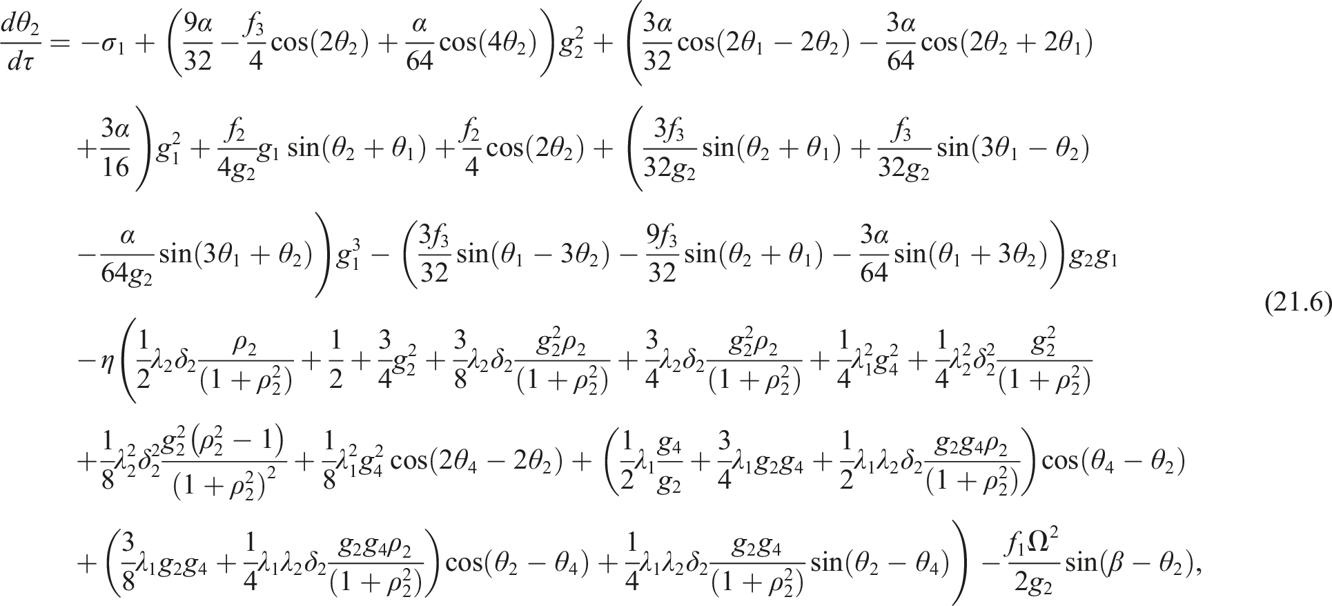
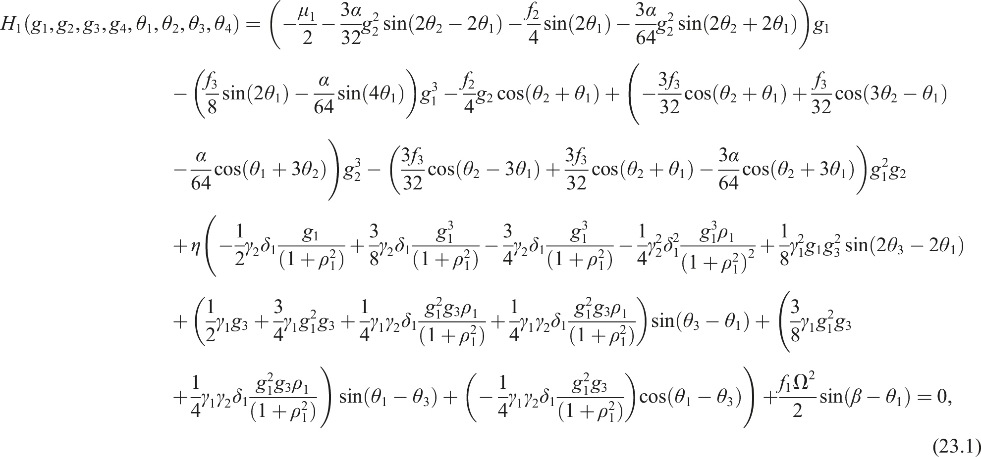
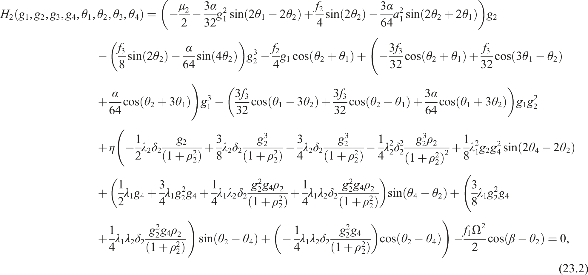
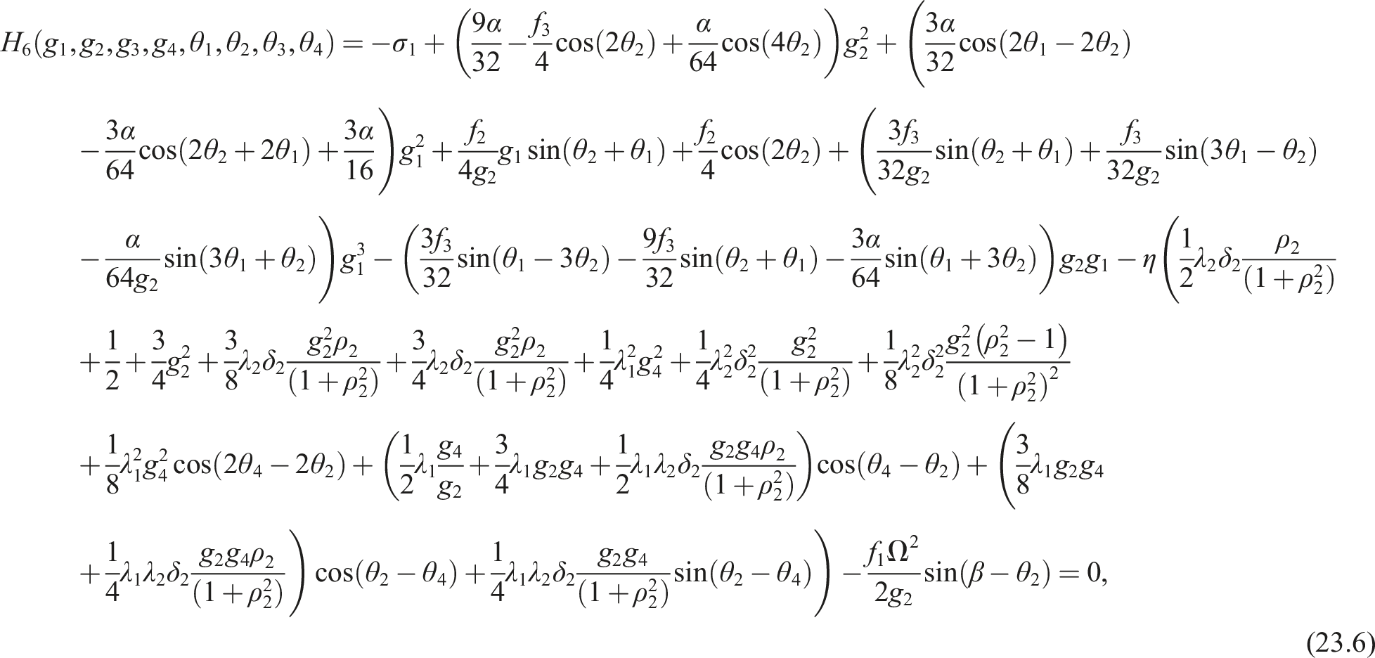
where $g_j\left(\tau \right),{\theta }_j\left(\tau \right),\left\{j=1,2,\dots ,6\right\}$ are the oscillation amplitudes and the phase angles of the two-pole rotor model, $PPFC$ , and $IRC$ , respectively. It is important to note that $g_j\left(\tau \right)$ and ${\theta }_j\left(\tau \right),\left\{j=1,2,3,4\right\}$ are governed by the autonomous nonlinear system given by equations (21.1)–(21.6). In addition, $g_j\left(\tau \right),{\theta }_j\left(\tau \right),\left\{j=5,4\right\}$ depend on $g_j\left(\tau \right)$ and ${\theta }_j\left(\tau \right),\left\{j=1,2\right\}$ such that $g_5={\delta }_1{g}_1/\sqrt{{\delta }_1^2+1},g_6={\delta }_2{g}_2/\sqrt{{\delta }_2^2+1},{\theta }_5={\theta }_1-{\tan }^{-1}\left({\rho }_1\right)$ , and ${\theta }_6={\theta }_2-{\tan }^{-1}\left({\rho }_2\right)$ . Therefore, by analyzing the dynamical system given equations (21.1)–(21.6), one can investigate the bifurcation behaviors of the system given by equations (11.1)–(11.6).

Steady-state solution and stability analysis

Based on equations (22.1)–(22.6), the steady-state periodic motion of the closed-loop dynamical system, described by equations (11.1)–(11.6), occur when the rate of change of the oscillation amplitudes ( $g_j\left(\tau \right)$ ) and corresponding phase angles $\left({\theta }_j\left(\tau \right)\right)$ is zero, where $j=1,2,\dots ,4$ . This means that ${dg}_j/d\tau =d{\theta }_j/d\tau =0,\left\{j=1,2,3,4\right\}$ . Inserting this condition into equations (22.1)–(22.6), yields

$\begin{array}{l}{H}_1\left(g_1,g_2,g_3,g_4,{\theta }_1,{\theta }_2,{\theta }_3,{\theta }_4\right)=\left(-\frac{{\mu }_1}{2}-\frac{3\alpha }{32}{g}_2^2\hspace{0.17em}\sin \left(2{\theta }_2-2{\theta }_1\right)-\frac{f_2}{4}\sin \left(2{\theta }_1\right)-\frac{3\alpha }{64}{g}_2^2\hspace{0.17em}\sin \left(2{\theta }_2+2{\theta }_1\right)\right)g_1\\ -(\frac{f_3}{8}\sin \left(2{\theta }_1\right)-\frac{\alpha }{64}\sin \left(4{\theta }_1\right))g_1^3-\frac{f_2}{4}{g}_2\hspace{0.17em}\cos \left({\theta }_2+{\theta }_1\right)+(-\frac{3f_3}{32}\cos \left({\theta }_2+{\theta }_1\right)+\frac{f_3}{32}\cos \left(3{\theta }_2-{\theta }_1\right)\\ -\frac{\alpha }{64}\cos \left({\theta }_1+3{\theta }_2\right))g_2^3-\left(\frac{3f_3}{32}\cos \left({\theta }_2-3{\theta }_1\right)+\frac{3f_3}{32}\cos \left({\theta }_2+{\theta }_1\right)-\frac{3\alpha }{64}\cos \left({\theta }_2+3{\theta }_1\right)\right)g_1^2{g}_2\\ +\eta (-\frac{1}{2}{\gamma }_2{\delta }_1\frac{g_1}{\left(1+{\rho }_1^2\right)}+\frac{3}{8}{\gamma }_2{\delta }_1\frac{g_1^3}{\left(1+{\rho }_1^2\right)}-\frac{3}{4}{\gamma }_2{\delta }_1\frac{g_1^3}{\left(1+{\rho }_1^2\right)}-\frac{1}{4}{\gamma }_2^2{\delta }_1^2\frac{g_1^3{\rho }_1}{{\left(1+{\rho }_1^2\right)}^2}+\frac{1}{8}{\gamma }_1^2{g}_1{g}_3^2\hspace{0.17em}\sin \left(2{\theta }_3-2{\theta }_1\right)\\ +(\frac{1}{2}{\gamma }_1{g}_3+\frac{3}{4}{\gamma }_1{g}_1^2{g}_3+\frac{1}{4}{\gamma }_1{\gamma }_2{\delta }_1\frac{g_1^2{g}_3{\rho }_1}{\left(1+{\rho }_1^2\right)}+\frac{1}{4}{\gamma }_1{\gamma }_2{\delta }_1\frac{g_1^2{g}_3{\rho }_1}{\left(1+{\rho }_1^2\right)})\sin \left({\theta }_3-{\theta }_1\right)+(\frac{3}{8}{\gamma }_1{g}_1^2{g}_3\\ +\frac{1}{4}{\gamma }_1{\gamma }_2{\delta }_1\frac{g_1^2{g}_3{\rho }_1}{\left(1+{\rho }_1^2\right)})\hspace{0.17em}\sin \left({\theta }_1-{\theta }_3\right)+\left(-\frac{1}{4}{\gamma }_1{\gamma }_2{\delta }_1\frac{g_1^2{g}_3}{\left(1+{\rho }_1^2\right)}\right)\cos \left({\theta }_1-{\theta }_3\right))+\frac{f_1{\mathrm{\Omega }}^2}{2}\sin \left(\beta -{\theta }_1\right)=0,\end{array}$

(23.1)

$\begin{array}{l}{H}_2\left(g_1,g_2,g_3,g_4,{\theta }_1,{\theta }_2,{\theta }_3,{\theta }_4\right)=\left(-\frac{{\mu }_2}{2}-\frac{3\alpha }{32}{g}_1^2\hspace{0.17em}\sin \left(2{\theta }_1-2{\theta }_2\right)+\frac{f_2}{4}\sin \left(2{\theta }_2\right)-\frac{3\alpha }{64}{a}_1^2\hspace{0.17em}\sin \left(2{\theta }_2+2{\theta }_1\right)\right)g_2\\ -(\frac{f_3}{8}\sin \left(2{\theta }_2\right)-\frac{\alpha }{64}\sin \left(4{\theta }_2\right))g_2^3-\frac{f_2}{4}{g}_1\hspace{0.17em}\cos \left({\theta }_2+{\theta }_1\right)+(-\frac{3f_3}{32}\cos \left({\theta }_2+{\theta }_1\right)+\frac{f_3}{32}\cos \left(3{\theta }_1-{\theta }_2\right)\\ +\frac{\alpha }{64}\cos \left({\theta }_2+3{\theta }_1\right))g_1^3-\left(\frac{3f_3}{32}\cos \left({\theta }_1-3{\theta }_2\right)+\frac{3f_3}{32}\cos \left({\theta }_2+{\theta }_1\right)+\frac{3\alpha }{64}\cos \left({\theta }_1+3{\theta }_2\right)\right)g_1{g}_2^2\\ +\eta (-\frac{1}{2}{\lambda }_2{\delta }_2\frac{g_2}{\left(1+{\rho }_2^2\right)}+\frac{3}{8}{\lambda }_2{\delta }_2\frac{g_2^3}{\left(1+{\rho }_2^2\right)}-\frac{3}{4}{\lambda }_2{\delta }_2\frac{g_2^3}{\left(1+{\rho }_2^2\right)}-\frac{1}{4}{\lambda }_2^2{\delta }_2^2\frac{g_2^3{\rho }_2}{{\left(1+{\rho }_2^2\right)}^2}+\frac{1}{8}{\lambda }_1^2{g}_2{g}_4^2\hspace{0.17em}\sin \left(2{\theta }_4-2{\theta }_2\right)\\ +(\frac{1}{2}{\lambda }_1{g}_4+\frac{3}{4}{\lambda }_1{g}_2^2{g}_4+\frac{1}{4}{\lambda }_1{\lambda }_2{\delta }_2\frac{g_2^2{g}_4{\rho }_2}{\left(1+{\rho }_2^2\right)}+\frac{1}{4}{\lambda }_1{\lambda }_2{\delta }_2\frac{g_2^2{g}_4{\rho }_2}{\left(1+{\rho }_2^2\right)})\sin \left({\theta }_4-{\theta }_2\right)+(\frac{3}{8}{\lambda }_1{g}_2^2{g}_4\\ +\frac{1}{4}{\lambda }_1{\lambda }_2{\delta }_2\frac{g_2^2{g}_4{\rho }_2}{\left(1+{\rho }_2^2\right)})\hspace{0.17em}\sin \left({\theta }_2-{\theta }_4\right)+\left(-\frac{1}{4}{\lambda }_1{\lambda }_2{\delta }_2\frac{g_2^2{g}_4}{\left(1+{\rho }_2^2\right)}\right)\cos \left({\theta }_2-{\theta }_4\right))-\frac{f_1{\mathrm{\Omega }}^2}{2}\cos \left(\beta -{\theta }_2\right)=0,\end{array}$

(23.2)

$H_3\left(g_1,g_2,g_3,g_4,{\theta }_1,{\theta }_2,{\theta }_3,{\theta }_4\right)=\left(\frac{-{\mu }_3}{2}\right)g_3+\left(\frac{{\zeta }_1}{2{\omega }_1}\sin \left({\theta }_1-{\theta }_3\right)\right)g_1=0,$

(23.3)

$H_4\left(g_1,g_2,g_3,g_4,{\theta }_1,{\theta }_2,{\theta }_3,{\theta }_4\right)=\left(\frac{-{\mu }_4}{2}\right)g_4+\left(\frac{{\zeta }_2}{2{\omega }_2}\sin \left({\theta }_2-{\theta }_4\right)\right)g_2=0,$

(23.4)

$\begin{array}{l}{H}_5\left(g_1,g_2,g_3,g_4,{\theta }_1,{\theta }_2,{\theta }_3,{\theta }_4\right)=-{\sigma }_1+\left(\frac{9\alpha }{32}-\frac{f_3}{4}\cos \left(2{\theta }_1\right)+\frac{\alpha }{64}\cos \left(4{\theta }_1\right)\right)g_1^2+(\frac{3\alpha }{32}\cos \left(2{\theta }_2-2{\theta }_1\right)\\ -\frac{3\alpha }{64}\cos \left(2{\theta }_2+2{\theta }_1\right)+\frac{3\alpha }{16})g_2^2-\frac{f_2}{4}\cos \left(2{\theta }_1\right)+\frac{f_2}{4g_1}{g}_2\hspace{0.17em}\sin \left({\theta }_2+{\theta }_1\right)+(\frac{3f_3}{32g_1}\sin \left({\theta }_2+{\theta }_1\right)+\frac{f_3}{32g_1}\sin \left(3{\theta }_2-{\theta }_1\right)\\ +\frac{\alpha }{64g_1}\sin \left({\theta }_1+3{\theta }_2\right))g_2^3-\left(\frac{3f_3}{32}\sin \left({\theta }_2-3{\theta }_1\right)-\frac{9f_3}{32}\sin \left({\theta }_2+{\theta }_1\right)+\frac{3\alpha }{64}\sin \left({\theta }_2+3{\theta }_1\right)\right)g_1{g}_2-\eta (\frac{1}{2}{\gamma }_2{\delta }_1\frac{{\rho }_1}{\left(1+{\rho }_1^2\right)}\\ +\frac{1}{2}+\frac{3}{4}{g}_1^2+\frac{3}{8}{\gamma }_2{\delta }_1\frac{g_1^2{\rho }_1}{\left(1+{\rho }_1^2\right)}+\frac{3}{4}{\gamma }_2{\delta }_1\frac{g_1^2{\rho }_1}{\left(1+{\rho }_1^2\right)}+\frac{1}{4}{\gamma }_1^2{g}_3^2+\frac{1}{4}{\gamma }_2^2{\delta }_1^2\frac{g_1^2}{\left(1+{\rho }_1^2\right)}+\frac{1}{8}{\gamma }_2^2{\delta }_1^2\frac{g_1^2\left({\rho }_1^2-1\right)}{{\left(1+{\rho }_1^2\right)}^2}\\ +\frac{1}{8}{\gamma }_1^2{g}_3^2\hspace{0.17em}\cos \left(2{\theta }_3-2{\theta }_1\right)+(\frac{1}{2}{\gamma }_1\frac{g_3}{g_1}+\frac{3}{4}{\gamma }_1{g}_1{g}_3+\frac{1}{2}{\gamma }_1{\gamma }_2{\delta }_1\frac{g_1{g}_3{\rho }_1}{\left(1+{\rho }_1^2\right)})\cos \left({\theta }_3-{\theta }_1\right)+(\frac{3}{8}{\gamma }_1{g}_1{g}_3\\ +\frac{1}{4}{\gamma }_1{\gamma }_2{\delta }_1\frac{g_1{g}_3{\rho }_1}{\left(1+{\rho }_1^2\right)})\hspace{0.17em}\cos \left({\theta }_1-{\theta }_3\right)+\frac{1}{4}{\gamma }_1{\gamma }_2{\delta }_1\frac{g_1{g}_3}{\left(1+{\rho }_1^2\right)}\sin \left({\theta }_1-{\theta }_3\right))-\frac{f_1{\mathrm{\Omega }}^2}{2g_1}\cos \left(\beta -{\theta }_1\right)=0,\end{array}$

(23.5)

$\begin{array}{l}{H}_6\left(g_1,g_2,g_3,g_4,{\theta }_1,{\theta }_2,{\theta }_3,{\theta }_4\right)=-{\sigma }_1+\left(\frac{9\alpha }{32}-\frac{f_3}{4}\cos \left(2{\theta }_2\right)+\frac{\alpha }{64}\cos \left(4{\theta }_2\right)\right)g_2^2+(\frac{3\alpha }{32}\cos \left(2{\theta }_1-2{\theta }_2\right)\\ -\frac{3\alpha }{64}\cos \left(2{\theta }_2+2{\theta }_1\right)+\frac{3\alpha }{16})g_1^2+\frac{f_2}{4g_2}{g}_1\hspace{0.17em}\sin \left({\theta }_2+{\theta }_1\right)+\frac{f_2}{4}\cos \left(2{\theta }_2\right)+(\frac{3f_3}{32g_2}\sin \left({\theta }_2+{\theta }_1\right)+\frac{f_3}{32g_2}\sin \left(3{\theta }_1-{\theta }_2\right)\\ -\frac{\alpha }{64g_2}\sin \left(3{\theta }_1+{\theta }_2\right))g_1^3-\left(\frac{3f_3}{32}\sin \left({\theta }_1-3{\theta }_2\right)-\frac{9f_3}{32}\sin \left({\theta }_2+{\theta }_1\right)-\frac{3\alpha }{64}\sin \left({\theta }_1+3{\theta }_2\right)\right)g_2{g}_1-\eta (\frac{1}{2}{\lambda }_2{\delta }_2\frac{{\rho }_2}{\left(1+{\rho }_2^2\right)}\\ +\frac{1}{2}+\frac{3}{4}{g}_2^2+\frac{3}{8}{\lambda }_2{\delta }_2\frac{g_2^2{\rho }_2}{\left(1+{\rho }_2^2\right)}+\frac{3}{4}{\lambda }_2{\delta }_2\frac{g_2^2{\rho }_2}{\left(1+{\rho }_2^2\right)}+\frac{1}{4}{\lambda }_1^2{g}_4^2+\frac{1}{4}{\lambda }_2^2{\delta }_2^2\frac{g_2^2}{\left(1+{\rho }_2^2\right)}+\frac{1}{8}{\lambda }_2^2{\delta }_2^2\frac{g_2^2\left({\rho }_2^2-1\right)}{{\left(1+{\rho }_2^2\right)}^2}\\ +\frac{1}{8}{\lambda }_1^2{g}_4^2\hspace{0.17em}\cos \left(2{\theta }_4-2{\theta }_2\right)+(\frac{1}{2}{\lambda }_1\frac{g_4}{g_2}+\frac{3}{4}{\lambda }_1{g}_2{g}_4+\frac{1}{2}{\lambda }_1{\lambda }_2{\delta }_2\frac{g_2{g}_4{\rho }_2}{\left(1+{\rho }_2^2\right)})\cos \left({\theta }_4-{\theta }_2\right)+(\frac{3}{8}{\lambda }_1{g}_2{g}_4\\ +\frac{1}{4}{\lambda }_1{\lambda }_2{\delta }_2\frac{g_2{g}_4{\rho }_2}{\left(1+{\rho }_2^2\right)})\hspace{0.17em}\cos \left({\theta }_2-{\theta }_4\right)+\frac{1}{4}{\lambda }_1{\lambda }_2{\delta }_2\frac{g_2{g}_4}{\left(1+{\rho }_2^2\right)}\sin \left({\theta }_2-{\theta }_4\right))-\frac{f_1{\mathrm{\Omega }}^2}{2g_2}\sin \left(\beta -{\theta }_2\right)=0,\end{array}$

(23.6)

$H_7\left(g_1,g_2,g_3,g_4,{\theta }_1,{\theta }_2,{\theta }_3,{\theta }_4\right)={\sigma }_2-{\sigma }_1-\left(\frac{{\zeta }_1}{2g_3{\omega }_1}\cos \left({\theta }_1-{\theta }_3\right)\right)g_1=0,$

(23.7)

$H_8\left(g_1,g_2,g_3,g_4,{\theta }_1,{\theta }_2,{\theta }_3,{\theta }_4\right)={\sigma }_3-{\sigma }_1-\left(\frac{{\zeta }_2}{2g_4{\omega }_2}\cos \left({\theta }_2-{\theta }_4\right)\right)g_2=0.$

(23.8)

By solving $H_j\left(g_1,g_2,g_{3\hspace{0.17em}},g_{4\hspace{0.17em}},{\theta }_1,{\theta }_2,{\theta }_3,{\theta }_4\hspace{0.17em}\right)=0,\left\{j=1,2,\dots ,8\right\}$ in terms of a specific parameter of the system (i.e., ${\sigma }_1,f_1,f_2,$ or $f_3$ ) as a bifurcation parameter with fixing the others constant, one can obtain the response curves shown in the following section. In addition, to explore the solution stability along the evolution of the bifurcation parameter, suppose the solution $H_j\left(g_1,g_2,g_{3\hspace{0.17em}},g_{4\hspace{0.17em}},{\theta }_1,{\theta }_2,{\theta }_3,{\theta }_4\hspace{0.17em}\right)=0,\left\{j=1,2,\dots ,8\right\}$ is $g_1=p_1,{g_2=p}_2,{g_3=p}_3,{g_4=p}_4,{\theta }_1=p_5,{\theta }_2=p_6,{\theta }_3=p_7,$ and ${\theta }_4=p_8$ . Also, let $p_{10},p_{20},p_{30}$ , $p_{40}$ , $p_{50}$ , $p_{60}$ , $p_{70}$ and $p_{80}$ are small infinitesimal increments in the solution $p_1,p_2,p_3,p_4,p_5,p_6,p_7,$ and $p_8$ such that the perturbed solution can be written as follows

$\begin{array}{c}{g}_1=p_1+p_{10},g_2=p_2+p_{20},g_3=p_3+p_{30},g_4=p_4+p_{40},\\ {\theta }_1=p_5+p_{50},{\theta }_2=p_6+p_{60},{\theta }_3=p_7+p_{70},{\theta }_4=p_8+p_{80},\\ \frac{d{g}_1}{d\tau }=\frac{d{p}_{10}}{d\tau },\frac{d{g}_2}{d\tau }=\frac{d{p}_{20}}{d\tau },\frac{d{g}_3}{d\tau }=\frac{d{p}_{30}}{d\tau },\frac{d{g}_4}{d\tau }=\frac{d{p}_{40}}{d\tau },\\ \frac{d{\theta }_1}{d\tau }=\frac{d{p}_{50}}{d\tau },\frac{d{\theta }_2}{d\tau }=\frac{d{p}_{60}}{d\tau },\frac{d{\theta }_3}{d\tau }=\frac{d{p}_{70}}{d\tau },\frac{d{\theta }_4}{d\tau }=\frac{d{p}_{80}}{d\tau }.\end{array}\}$

(24)

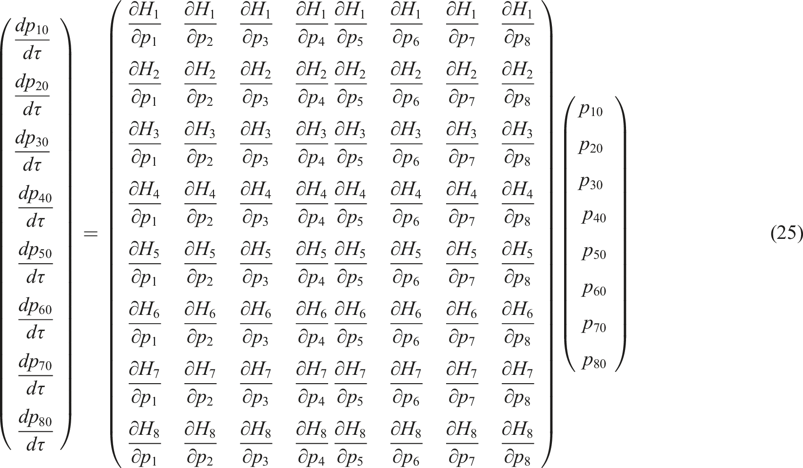
By inserting equation (24) into equations (23.1)–(23.8) with expanding for $p_{10},p_{20},p_{30}$ , $p_{40}$ , $p_{50}$ , $p_{60}$ , $p_{70}$ and $p_{80}$ keeping the linear terms only, yield the linear system ⁴⁸

$\left(\begin{array}{l}\frac{d{p}_{10}}{d\tau }\\ \frac{d{p}_{20}}{d\tau }\\ \frac{d{p}_{30}}{d\tau }\\ \begin{array}{l}\frac{d{p}_{40}}{d\tau }\\ \frac{d{p}_{50}}{d\tau }\\ \frac{d{p}_{60}}{d\tau }\\ \frac{d{p}_{70}}{d\tau }\\ \frac{d{p}_{80}}{d\tau }\end{array}\end{array}\right)=\left(\begin{array}{l}\begin{array}{llll}\frac{\partial H_1}{\partial p_1}& \frac{\partial H_1}{\partial p_2}& \frac{\partial H_1}{\partial p_3}& \frac{\partial H_1}{\partial p_4}\\ \frac{\partial H_2}{\partial p_1}& \frac{\partial H_2}{\partial p_2}& \frac{\partial H_2}{\partial p_3}& \frac{\partial H_2}{\partial p_4}\\ \frac{\partial H_3}{\partial p_1}& \frac{\partial H_3}{\partial p_2}& \frac{\partial H_3}{\partial p_3}& \frac{\partial H_3}{\partial p_4}\\ \frac{\partial H_4}{\partial p_1}& \frac{\partial H_4}{\partial p_2}& \frac{\partial H_4}{\partial p_3}& \frac{\partial H_4}{\partial p_4}\end{array}\begin{array}{llll}\frac{\partial H_1}{\partial p_5}& \frac{\partial H_1}{\partial p_6}& \frac{\partial H_1}{\partial p_7}& \frac{\partial H_1}{\partial p_8}\\ \frac{\partial H_2}{\partial p_5}& \frac{\partial H_2}{\partial p_6}& \frac{\partial H_2}{\partial p_7}& \frac{\partial H_2}{\partial p_8}\\ \frac{\partial H_3}{\partial p_5}& \frac{\partial H_3}{\partial p_6}& \frac{\partial H_3}{\partial p_7}& \frac{\partial H_3}{\partial p_8}\\ \frac{\partial H_4}{\partial p_5}& \frac{\partial H_4}{\partial p_6}& \frac{\partial H_4}{\partial p_7}& \frac{\partial H_4}{\partial p_8}\end{array}\\ \begin{array}{llll}\frac{\partial H_5}{\partial p_1}& \frac{\partial H_5}{\partial p_2}& \frac{\partial H_5}{\partial p_3}& \frac{\partial H_5}{\partial p_4}\\ \frac{\partial H_6}{\partial p_1}& \frac{\partial H_6}{\partial p_2}& \frac{\partial H_6}{\partial p_3}& \frac{\partial H_6}{\partial p_4}\\ \frac{\partial H_7}{\partial p_1}& \frac{\partial H_7}{\partial p_2}& \frac{\partial H_7}{\partial p_3}& \frac{\partial H_7}{\partial p_4}\\ \frac{\partial H_8}{\partial p_1}& \frac{\partial H_8}{\partial p_2}& \frac{\partial H_8}{\partial p_3}& \frac{\partial H_8}{\partial p_4}\end{array}\begin{array}{llll}\frac{\partial H_5}{\partial p_5}& \frac{\partial H_5}{\partial p_6}& \frac{\partial H_5}{\partial p_7}& \frac{\partial H_5}{\partial p_8}\\ \frac{\partial H_6}{\partial p_5}& \frac{\partial H_6}{\partial p_6}& \frac{\partial H_6}{\partial p_7}& \frac{\partial H_6}{\partial p_8}\\ \frac{\partial H_7}{\partial p_5}& \frac{\partial H_7}{\partial p_6}& \frac{\partial H_7}{\partial p_7}& \frac{\partial H_7}{\partial p_8}\\ \frac{\partial H_8}{\partial p_5}& \frac{\partial H_8}{\partial p_6}& \frac{\partial H_8}{\partial p_7}& \frac{\partial H_8}{\partial p_8}\end{array}\end{array}\right)\left(\begin{array}{l}{p}_{10}\\ p_{20}\\ p_{30}\\ \begin{array}{l}{p}_{40}\\ p_{50}\\ p_{60}\\ p_{70}\\ p_{80}\end{array}\end{array}\right)$

(25)

where $\partial H_j/\partial p_k,\left\{j=1,2\dots ,8;\hspace{0.17em}k=1,2,\dots ,8\right\}$ are the Jacobian matrix of the right-hand side of equations (23.1)–(23.8) about the equilibrium point $\left(p_1,p_2,p_3,p_4,p_5,p_6,p_7,p_8\right)$ . For this hyperbolic equilibrium point, the linear and nonlinear systems given by Equations (21.1)–(21.8) and (25) are topologically equivalent. ⁶⁰ Consequently, the solution stability of Equations (23.1)–(23.8), can be explored based on the eigenvalues of equation (25).

Response curves and numerical simulations

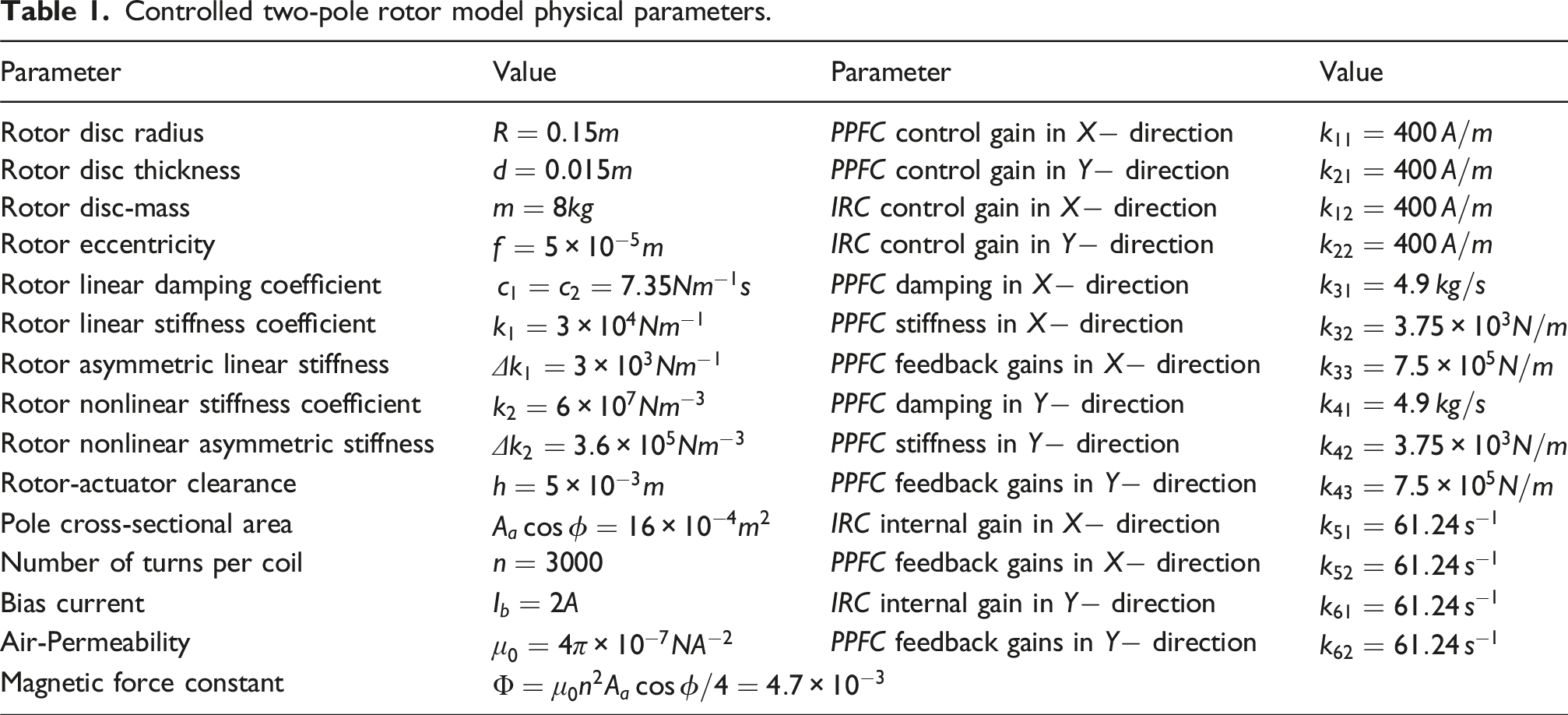
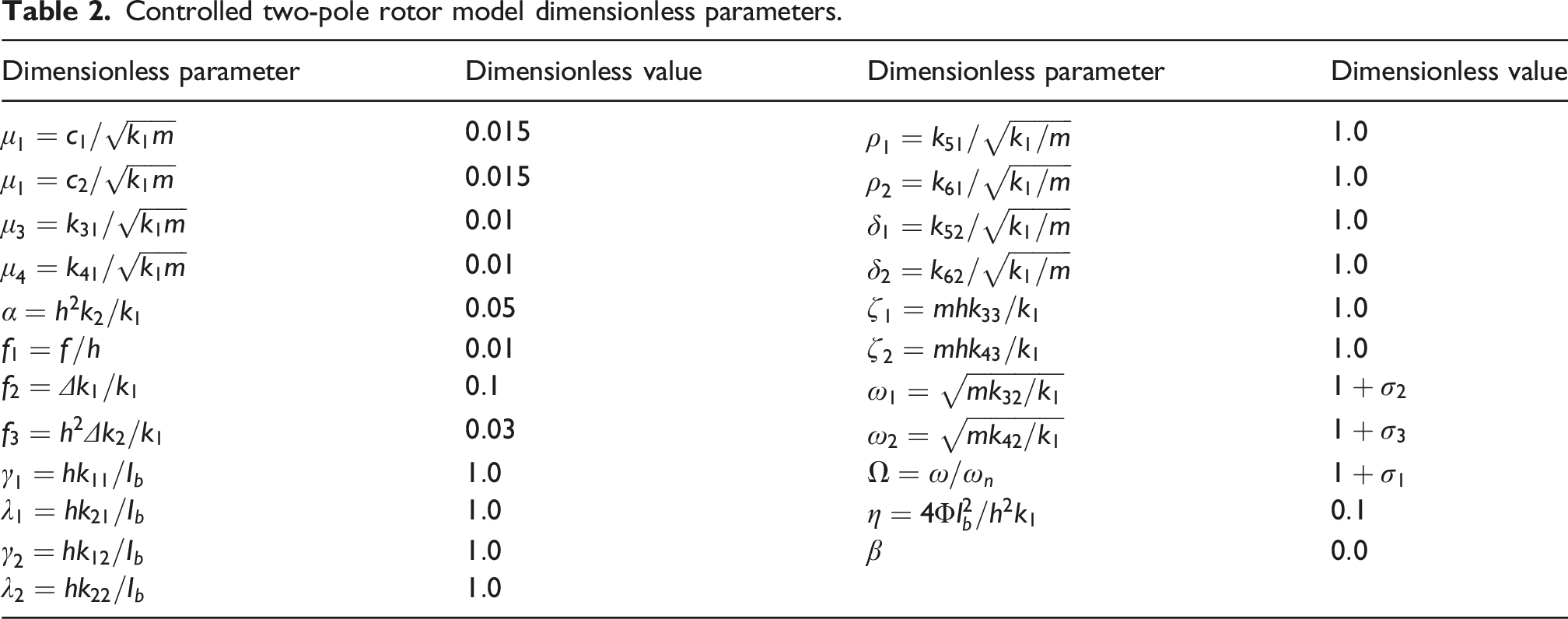
As the main goal of this work is to investigate the performance of three controllers in suppressing the undesired vibration of the considered two-pole rotor model, this section is organized such that the dynamics of the rotor model have been explored first when the three controllers are turned off. Then, the system dynamics under the $PPFC$ only (i.e., controller-1) have been investigated. After that, the rotor bifurcation behaviors under the $IRC$ only (i.e., controller-2) are studied. Subsequently, the performance of the combined controllers $PPFC+IRC$ (i.e., controller-3) on the two-pole rotor model oscillatory motion is examined. Finally, a comparison between the three introduced control methodologies has been made. Following the earlier analysis, the steady-state vibrational behaviors of the two-pole rotor model with the different control strategies given by equations (11.1)–(11.6), can be investigated utilizing Equation (23.1) –(23.8), and (25). The evolution of the steady-state oscillation amplitude $\left(g_j,j=1,2,\dots ,6\right)$ can be plotted against one of the system or control parameters (i.e., ${\sigma }_1,f_1,f_2,f_3,{\gamma }_1,{\gamma }_2,{\lambda }_1,{\lambda }_2,\dots etc$ ) as a main bifurcation coefficient, while fixing the other parameters constant. ⁶¹ At the same time, while plotting the bifurcation diagram branches, the solution stability of Equations (23.1)–(23.8) can be distinguished by exploring the eigenvalues of equation (25). To apply the proposed solution procedure, the actual physical parameters of a controlled two-pole rotor given by Equation (10.1)–(10.6), and the corresponding dimensionless system parameters of the normalized model given by Equation (11.1)–(11.6) as a case study are given in Tables 1 and 2, respectively. ⁴⁷

Table 1.

Controlled two-pole rotor model physical parameters.

Parameter	Value	Parameter	Value
Rotor disc radius	$R=0.15m$	$PPFC$ control gain in $X-$ direction	$k_{11}=400\hspace{0.17em}A/m$
Rotor disc thickness	$d=0.015m$	$PPFC$ control gain in $Y-$ direction	$k_{21}=400\hspace{0.17em}A/m$
Rotor disc-mass	$m=8kg$	$IRC$ control gain in $X-$ direction	$k_{12}=400\hspace{0.17em}A/m$
Rotor eccentricity	$f=5\times {10}^{-5}m$	$IRC$ control gain in $Y-$ direction	$k_{22}=400\hspace{0.17em}A/m$
Rotor linear damping coefficient	${\hspace{0.17em}c}_1=c_2=7.35{Nm}^{-1}s$	$PPFC$ damping in $X-$ direction	$k_{31}=4.9\hspace{0.17em}kg/s$
Rotor linear stiffness coefficient	$k_1=3\times {10}^4{Nm}^{-1}$	$PPFC$ stiffness in $X-$ direction	$k_{32}=3.75\times {10}^{3}N/m$
Rotor asymmetric linear stiffness	$\mathit{\Delta }{k}_1=3\times {10}^3{Nm}^{-1}$	$PPFC$ feedback gains in $X-$ direction	$k_{33}=7.5\times {10}^{5}N/m$
Rotor nonlinear stiffness coefficient	$k_2=6\times {10}^7{Nm}^{-3}$	$PPFC$ damping in $Y-$ direction	$k_{41}=4.9\hspace{0.17em}kg/s$
Rotor nonlinear asymmetric stiffness	${\mathit{\Delta }k}_2=3.6\times {10}^5{Nm}^{-3}$	$PPFC$ stiffness in $Y-$ direction	$k_{42}=3.75\times {10}^{3}N/m$
Rotor-actuator clearance	$h=5\times {10}^{-3}m$	$PPFC$ feedback gains in $Y-$ direction	$k_{43}=7.5\times {10}^{5}N/m$
Pole cross-sectional area	$A_a\hspace{0.17em}\cos \hspace{0.17em}\varphi =16\times {10}^{-4}{m}^2$	$IRC$ internal gain in $X-$ direction	$k_{51}=61.24\hspace{0.17em}{s}^{-1}$
Number of turns per coil	$n=3000$	$PPFC$ feedback gains in $X-$ direction	$k_{52}={61.24\hspace{0.17em}s}^{-1}$
Bias current	$I_b=2A$	$IRC$ internal gain in $Y-$ direction	$k_{61}=61.24\hspace{0.17em}{s}^{-1}$
Air-Permeability	${\mu }_0=4\pi \times {10}^{-7}{NA}^{-2}$	$PPFC$ feedback gains in $Y-$ direction	$k_{62}=61.24\hspace{0.17em}{s}^{-1}$
Magnetic force constant	$\mathrm{\Phi }={\mu }_0{n}^2{A}_a\hspace{0.17em}\cos \hspace{0.17em}\varphi /4=4.7\times {10}^{-3}$

Table 2.

Controlled two-pole rotor model dimensionless parameters.

Dimensionless parameter	Dimensionless value	Dimensionless parameter	Dimensionless value
${\mu }_1=c_1/\sqrt{k_{1}m}$	$0.015$	${\rho }_1=k_{51}/\sqrt{k_1/m}$	$1.0$
${\mu }_1=c_2/\sqrt{k_{1}m}$	$0.015$	${\rho }_2=k_{61}/\sqrt{k_1/m}$	$1.0$
${\mu }_3=k_{31}/\sqrt{k_{1}m}$	$0.01$	${\delta }_1=k_{52}/\sqrt{k_1/m}$	$1.0$
${\mu }_4=k_{41}/\sqrt{k_{1}m}$	$0.01$	${\delta }_2=k_{62}/\sqrt{k_1/m}$	$1.0$
$\alpha =h^2{k}_2/k_1$	$0.05$	${\zeta }_1=mh{k}_{33}/k_1$	$1.0$
$f_1=f/h$	$0.01$	${\zeta }_2=mh{k}_{43}/k_1$	$1.0$
$f_2=\mathit{\Delta }{k}_1/k_1$	$0.1$	${\omega }_1=\sqrt{m{k}_{32}/k_1}$	$1+{\sigma }_2$
$f_3=h^2\mathit{\Delta }{k}_2/k_1$	$0.03$	${\omega }_2=\sqrt{m{k}_{42}/k_1}$	$1+{\sigma }_3$
${\gamma }_1=h{k}_{11}/I_b$	$1.0$	$\mathrm{\Omega }=\omega /{\omega }_n$	$1+{\sigma }_1$
${\lambda }_1=h{k}_{21}/I_b$	$1.0$	$\eta =4\mathrm{\Phi }{I}_b^2/h^2{k}_1$	$0.1$
${\gamma }_2=h{k}_{12}/I_b$	$1.0$	$\beta$	$0.0$
${\lambda }_2=h{k}_{22}/I_b$	$1.0$

Uncontrolled two-pole rotor model

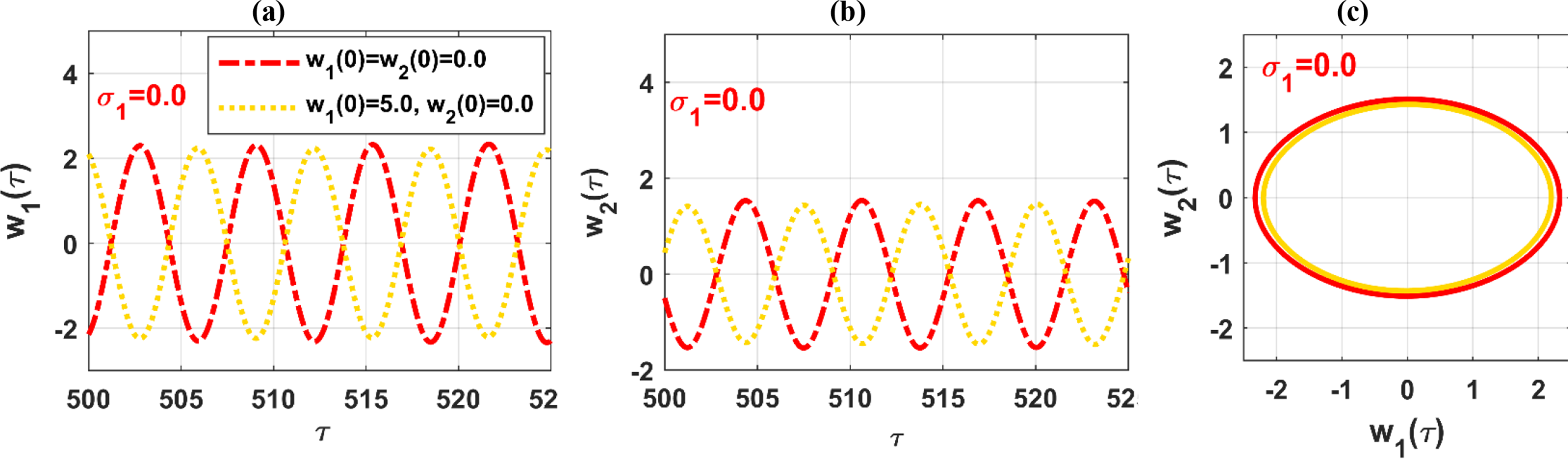
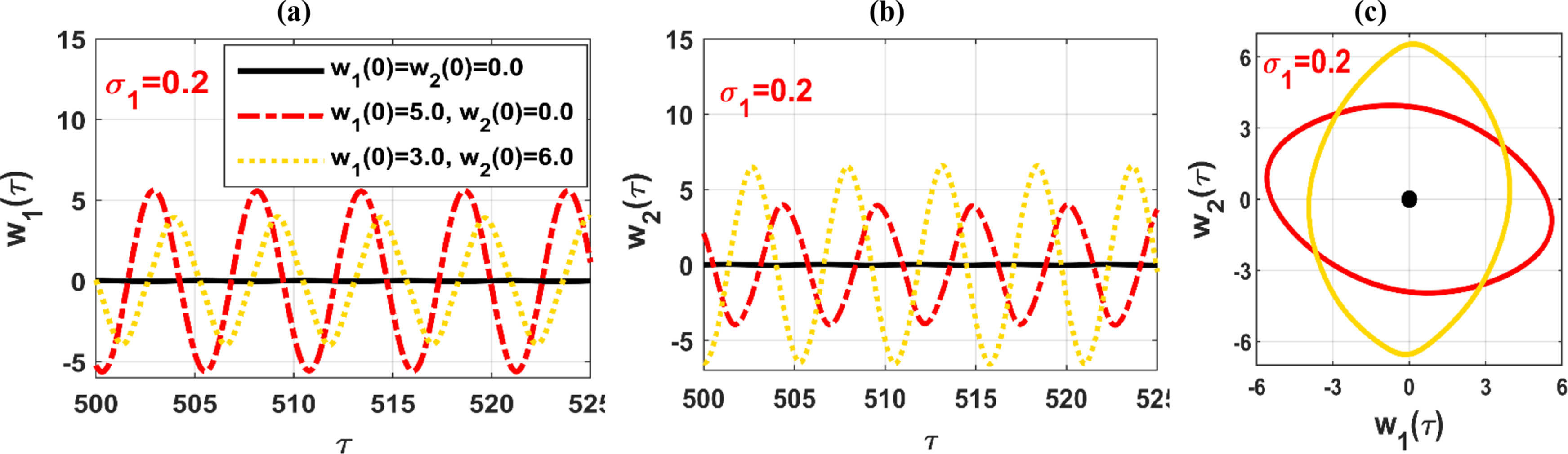
The dynamics of the considered two-pole rotor model are analyzed without control in this section by exploring the evolution of the oscillation amplitudes $g_1$ and $g_2$ under steady-state conditions with various rotor parameters. As the ${\sigma }_1$ parameter quantitatively determines the proximity of the two-pole rotor’s angular speed $\mathrm{\Omega }$ to its normalized natural frequency (i.e., $\mathrm{\Omega }=1+{\sigma }_1$ ), ${\sigma }_1$ is used as a bifurcation parameter to represent the rotor’s response near the primary resonance condition. In Figure 3, the evolution of $g_1$ and $g_2$ is explored against ${\sigma }_1$ when the rotor system is subjected to simultaneous external excitation (i.e., $f_1=0.01$ ), linear parametric excitation (i.e., $f_2=0.1$ ), and nonlinear parametric excitation (i.e., $f_3=0.03$ )). It is clear from the figure that complex motion bifurcation occurs in the two-pole rotor system near the primary resonance, where the system can exhibit monostable, bistable, or tri-stable periodic solutions depending on the angular speed. Additionally, the system may experience strong oscillation amplitudes, multi-stability, and jumping phenomena, leading to reduced efficiency and negative effects on both the rotor’s durability and reliability. To clarify the concept of a multi-stable periodic solution, examine Figure 3 around ${\sigma }_1=0.0$ . It can be observed that there are two stable solution branches (solid lines) that gradually merge into one as ${\sigma }_1$ increases, along with an unstable solution branch (dotted line). Mathematically, this indicates that the normalized dynamical system (11.1) and (11.2), when the controllers are decoupled (i.e., $\eta =0.0$ ), has two stable periodic solutions. The system responds with one of these solutions at a time depending on its initial state. To demonstrate the accuracy of Figure 3 when ${\sigma }_1=0.0$ , equations (11.1) and (11.2) were simulated numerically using the Runge–Kutta algorithm with two initial conditions: $w_1\left(0\right)=w_2\left(0\right)=0.0$ and $w_1\left(0\right)=0.5,w_2\left(0\right)=0.0$ , while keeping the initial velocities at zero. Figure 4 illustrates the existence of two periodic solutions with very similar oscillation amplitudes but with a ${\pi /2}^o$ phase difference, which agrees well with the bifurcation diagram in Figure 3. Furthermore, in Figure 3, it can be seen that the uncontrolled two-pole rotor model exhibits three simultaneous stable oscillation amplitudes when ${\sigma }_1=0.2$ . This implies that the normalized dynamical system (i.e., (11.1) and (11.2)) has three simultaneous stable periodic solutions when $\mathrm{\Omega }=1+0.2$ , with the rotor responding with one of these solutions depending on the initial conditions. To demonstrate this phenomenon, equations (11.1) and (11.2), with $\eta =0.0$ , were solved numerically, as shown in Figure 5, using three different initial positions: $w_1\left(0\right)=w_2\left(0\right)=0.0$ ; $w_1\left(0\right)=0.5,w_2\left(0\right)=0.0$ ; and $w_1\left(0\right)=3.0,w_2\left(0\right)=6.0$ , while keeping ${\dot{w}}_1\left(0\right)={\dot{w}}_2\left(0\right)=0.0$ . Figure 5 displays three stable periodic solutions with different amplitudes, which align accurately with the steady-state amplitudes $g_1$ and $g_2$ in Figure 3 when ${\sigma }_1=0.2$ .

Figure 3.

Evolution of $g_1$ and $g_2$ of the uncontrolled two-pole rotor model against ${\sigma }_1$ when $f_1=0.01,f_2=0.1,$ and $f_3=0.03$ .

Figure 4.

The existence of a bi-stable periodic solution of the uncontrolled two-pole rotor model when ${\sigma }_1=0.0$ (i.e., when $\mathrm{\Omega }=1.0$ ) according to the solutions bifurcation diagram in Figure 3.

Figure 5.

The existence of a tri-stable periodic solution of the uncontrolled two-pole rotor model when ${\sigma }_1=0.2$ (i.e., when $\mathrm{\Omega }=1.2$ ) according to the solutions bifurcation diagram in Figure 3.

To explore the rotor motion bifurcation in response to excitation force amplitudes, the evolution of $g_1$ and $g_2$ against $f_1,f_2,$ and $f_3$ are illustrated in Figures 6, 9, and 12, respectively, while keeping ${\sigma }_1=0.0$ . The evolution of $g_1$ and $g_2$ with increasing external excitation amplitude $f_1$ , using it as a bifurcation parameter while ${\sigma }_1=0.0,f_2=0.1,$ and $f_3=0.03$ , is depicted in Figure 6. The figure demonstrates the existence of a bistable solution for the two-pole rotor system as long as $f_1<0.06$ . However, increasing $f_1$ beyond $0.06$ results in a monotonic increase in monostable oscillations.

Figure 6.

Evolution of $g_1$ and $g_2$ of the uncontrolled two-pole rotor model against $f_1$ when ${\sigma }_1=0.0,f_2=0.1,$ and $f_3=0.03$ .

To numerically demonstrate the existence of bi-stability in the rotor system when $f_1<0.06$ , and the disappearance of this bi-stability, leading to monostable oscillations under strong external excitation (i.e., $f_1>0.06$ ), three basins of attraction in the $w_1\left(0\right)-w_2\left(0\right)$ plane, while fixing the velocities ${\dot{w}}_1\left(0\right)={\dot{w}}_2\left(0\right)=0.0$ , have been established by numerically integrating equations (11.1) and (11.2) for $f_1=0.03,0.05,$ and $0.1$ , as shown in Figures 7(a)–7(c), respectively. The red region refers to the basin of the high oscillation amplitude solution, while the yellow region indicates the basin of the low oscillation amplitude solution. By comparing Figures 6 and 7, one can infer the accurate correspondence between them, as the two-pole rotor model exhibits bi-stability when $f_1=0.03$ and $0.05$ (i.e., $f_1>0.06$ ), as shown in Figures 7(a) and 7(b). Additionally, Figure 7(c) shows the monostable basin of attraction of the two-pole rotor model when $f_1=0.1$ , which aligns accurately with the bifurcation diagram in Figure 6. In Figure 8, the steady-state time response of the two-pole rotor system has been simulated by integrating equations (11.1) and (11.2) when ${\sigma }_1=0.0,f_1=0.05,f_2=0.1,$ and $f_3=0.03$ , corresponding to Figure 7(b). Two initial conditions are selected: one within the red region (i.e., $w_1\left(0\right)=w_2\left(0\right)=0.0$ ) and the other within the yellow region (i.e., $w_1\left(0\right)=-2.0,w_2\left(0\right)=0.0$ ). The figure clearly shows that the system performs one of two periodic motions depending on the initial conditions, confirming the bi-stability.

Figure 7.

Basins of attraction of the uncontrolled two-pole rotor system solutions in $w_1\left(0\right)-w_2\left(0\right)$ space established according to Figure 6 when $f_1=0.03,0.05,$ and $0.1$ .

Figure 8.

The existence of a bi-stable periodic solution of the uncontrolled two-pole rotor model when $f_1=0.05,{\sigma }_1=0.0$ according to the solutions bifurcation diagram in Figure 6 and basins of attraction in Figure 7(b).

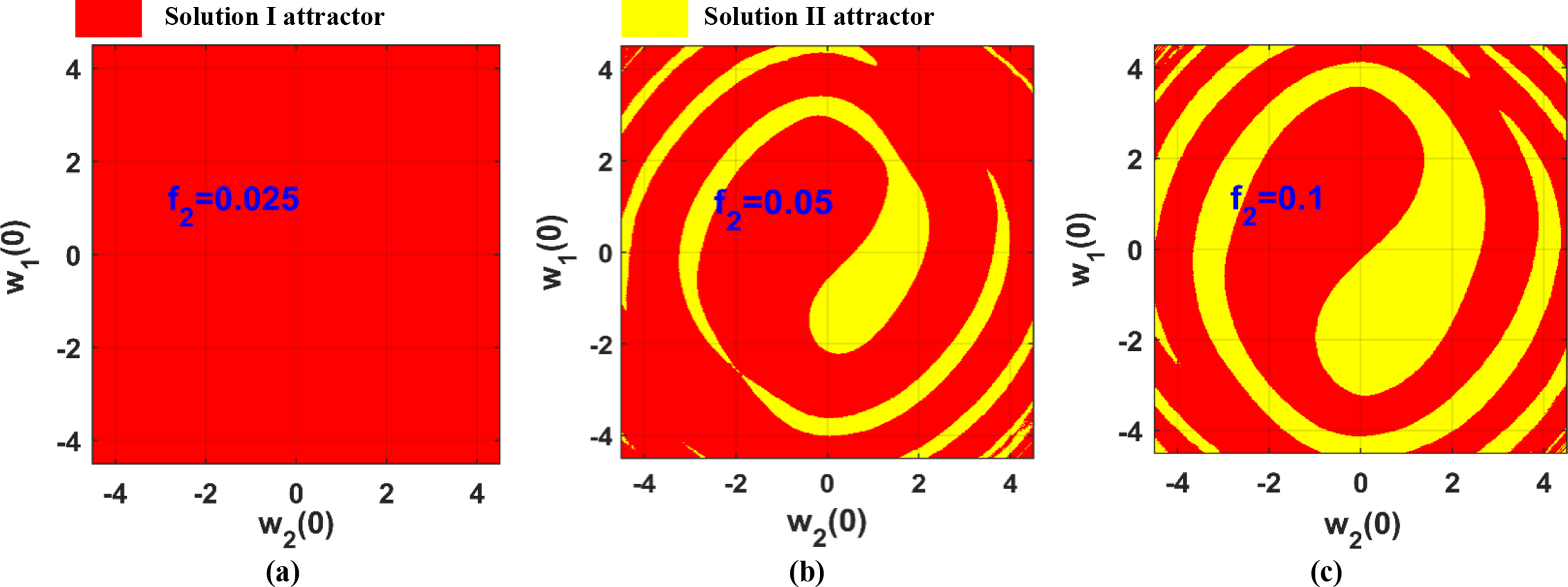
In Figure 9, the evolution of $g_1$ and $g_2$ against the linear parametric excitation force $f_2$ is explored while keeping ${\sigma }_1=0.0,f_1=0.01,$ and $f_3=0.03$ constant. The figure shows that the two-pole rotor system exhibits a monostable periodic solution as long as $f_2<0.04$ . However, increasing $f_2$ beyond $0.04$ results in a monotonic increase in the system’s vibration amplitudes, along with the emergence of bi-stability characteristics. To validate the accuracy of Figure 9, three basins of attraction are established in the $w_1\left(0\right)-w_2\left(0\right)$ space, with the rotor’s initial velocities set to zero (i.e., ${\dot{w}}_1\left(0\right)={\dot{w}}_2\left(0\right)=0.0$ ). This is done by numerically integrating equations (11.1) and (11.2) when $f_2=0.025,0.05,$ and $0.1$ , as shown in Figures 10(a)–10(c), respectively. Figure 10(a) demonstrates that the two-pole system has a single basin of attraction when $f_2=0.025$ , which aligns perfectly with Figure 9, where there is a single solution branch corresponding to a monostable periodic motion. Conversely, Figures 10(b) and 10(c) reveal the presence of two basins of attraction when $f_2=0.05$ and $0.1$ , respectively, which also agree with Figure 9, where two solution branches correspond to a bi-stable periodic motion of the two-pole rotor model at $f_2=0.05$ and $0.1$ . As illustrated in Figures 9 and 10(c), the steady-state time response of the rotor system has been simulated in Figure 11 by numerically solving equations (11.1) and (11.2) with $f_2=0.05$ . Two distinct initial conditions were considered: the first positioned within the red basin of attraction (i.e., $w_1\left(0\right)=w_2\left(0\right)=0.0$ ), and the second within the yellow basin (i.e., $w_1\left(0\right)=0.0,w_2\left(0\right)=2.0$ ). The results in Figure 11 indicate that the system follows one of two periodic motion states, contingent on the initial conditions, thereby confirming the presence of bi-stability. The evolution of $g_1$ and $g_2$ for the uncontrolled two-pole rotor model is plotted against the nonlinear parametric excitation amplitude $f_3$ , as shown in Figure 12. The figure reveals the presence of bistable periodic motion along the $f_3$ axis, where the rotor’s response depends on its initial conditions. Additionally, it is evident that both $g_1$ and $g_2$ exhibit a monotonic increase as $f_3$ grows.

Figure 9.

Evolution of $g_1$ and $g_2$ of the uncontrolled two-pole rotor model against $f_2$ when ${\sigma }_1=0.0,f_1=0.01,$ and $f_3=0.03$ .

Figure 10.

Basins of attraction of the uncontrolled two-pole rotor system solutions in $w_1\left(0\right)-w_2\left(0\right)$ space established according to Figure 9 when $f_2=0.025,0.05,$ and $0.1$ .

Figure 11.

The existence of a bi-stable periodic solution of the uncontrolled two-pole rotor model when $f_2=0.05,{\sigma }_1=0.0$ according to the solutions bifurcation diagram in Figure 9 and basins of attraction in Figure 10(b).

Figure 12.

Evolution of $g_1$ and $g_2$ of the uncontrolled two-pole rotor model against $f_3$ when ${\sigma }_1=0.0,f_1=0.01,$ and $f_2=0.1$ .

From the preceding analysis, it is clear that the asymmetric two-pole rotor model is prone to multi-stability and large-amplitude oscillations, both of which can significantly compromise the system’s efficiency, durability, and reliability. Consequently, the main objective of this work is to propose a streamlined and effective control strategy aimed at eliminating the unwanted bifurcations highlighted in Figures 3–12 and mitigating the oscillation amplitudes of $g_1$ and $g_2$ . To achieve this, the performance of three control methods $—PPFC,IRC,$ and a combined $PPFC+IRC$ approach $—$ has been thoroughly examined, leading to the identification of the optimal control strategy for suppressing undesired behaviors and stabilizing the system.

Rotor dynamics under controller-1: PPFC

This is the first time the $PPFC$ has been applied to mitigate the nonlinear oscillations of a system subjected to simultaneous external ( $f_1$ ), linear parametric ( $f_2$ ), and nonlinear parameter ( $f_3$ ) excitations. When the $PPFC$ is integrated solely into the two-pole system, the control current described by equations (7.1) and (7.2) simplifies to $I_x=-k_{11}{u}_1\left(t\right)$ and $I_y=-k_{21}{u}_2\left(t\right)$ , where $k_{12}=k_{22}=0.0$ . Additionally, the normalized equations governing the two-pole system’s dynamics, along with the $PPFC$ , reduce to Eqs. (11.1)–(11.4), with the dimensionless control gains for the $PPFC$ defined as ${\gamma }_1=h{k}_{11}/I_b$ and ${\lambda }_1=h{k}_{21}/I_b$ . In this subsection, the evolution of the rotor and $PPFC$ oscillation amplitudes (i.e., $g_1,g_2,g_3,$ and $g_4$ ) is analyzed in terms of the control gains ${\gamma }_1$ and ${\lambda }_1$ by solving the algebraic system given in Equations (23.1)–(23.8).

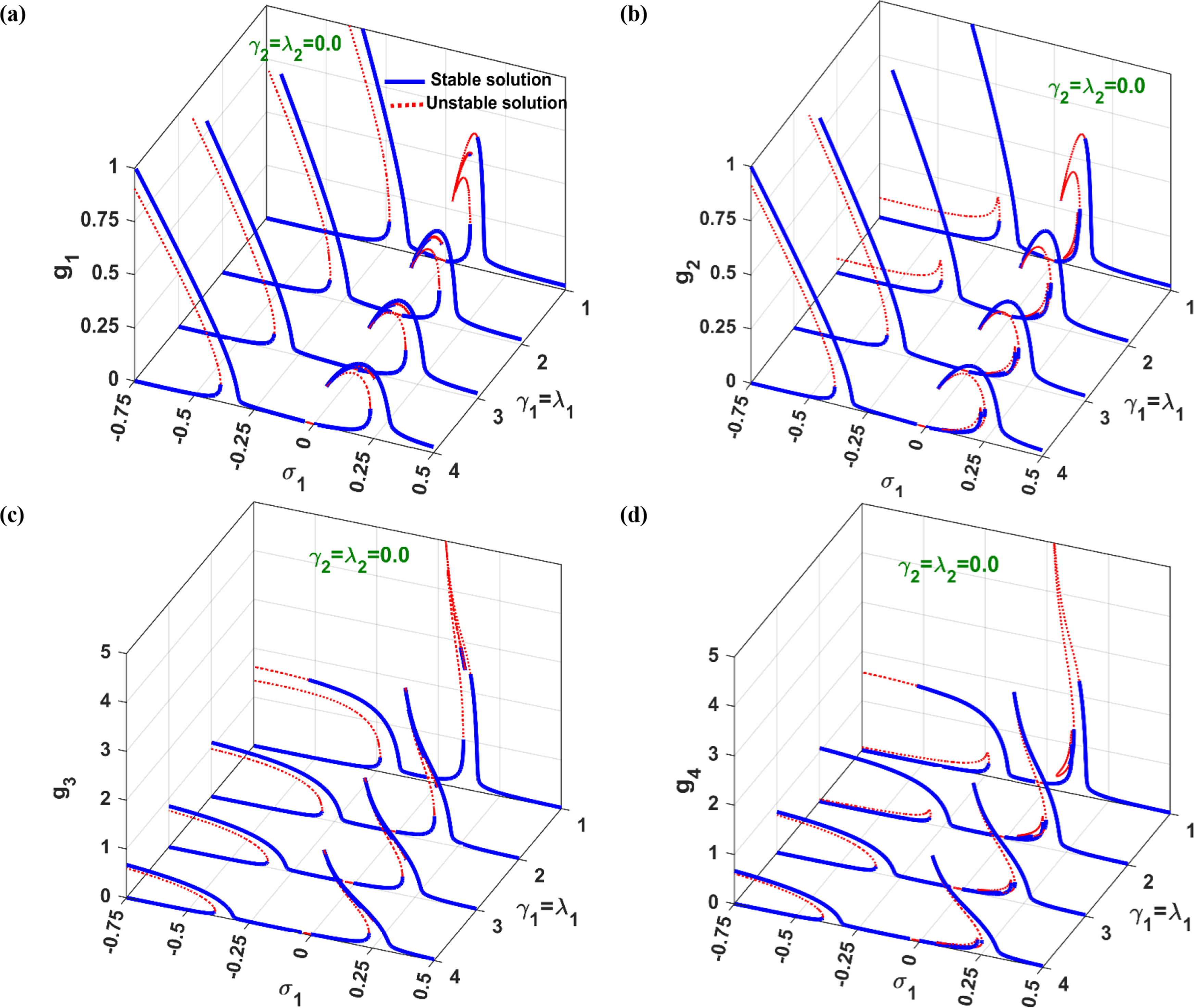
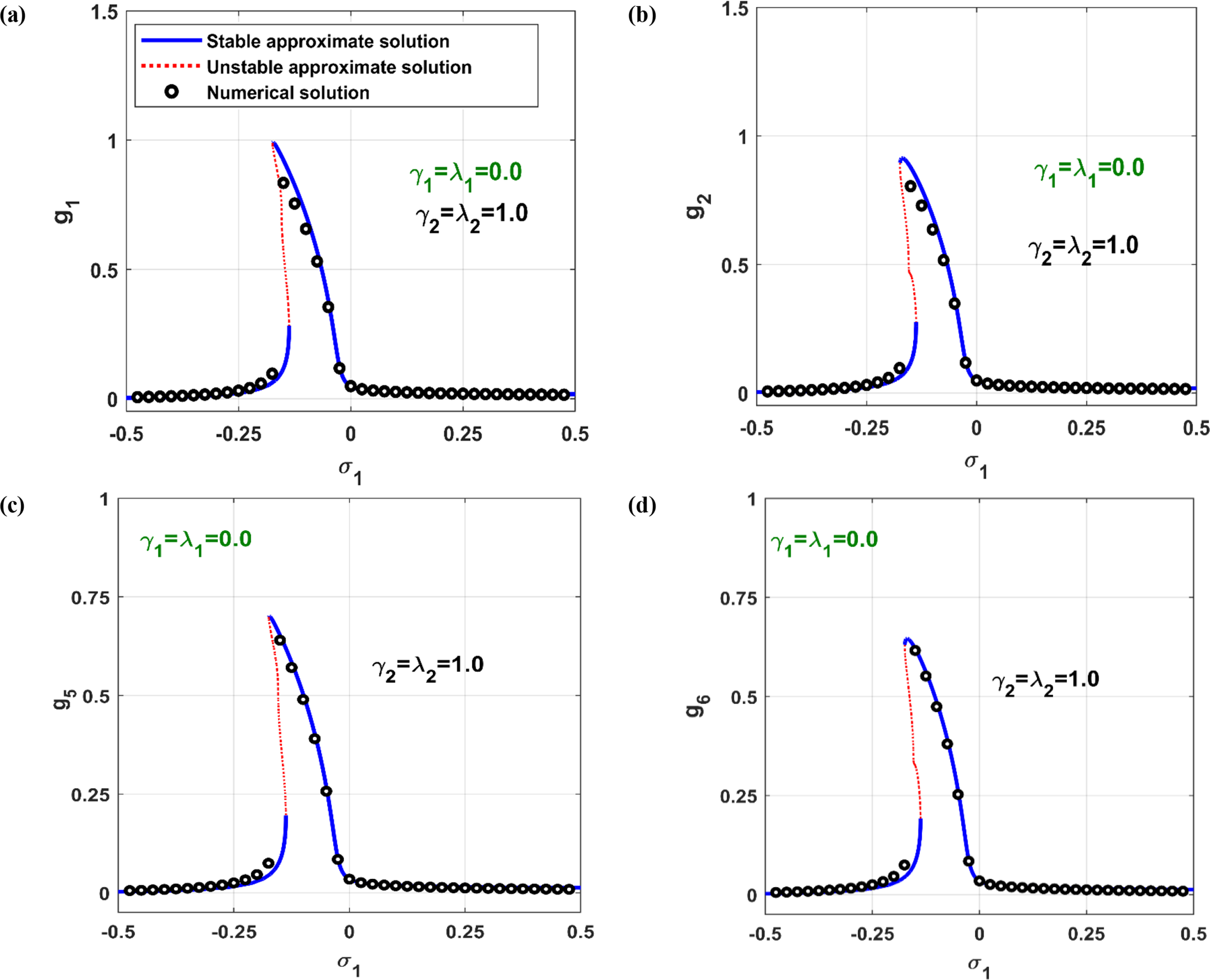
The steady-state amplitudes of both the two-pole system (i.e., $g_1$ and $g_2$ ) and the coupled $PPFC$ ((i.e., $g_3$ and $g_4$ ) as functions of ${\sigma }_1$ are illustrated in Figure 13. Comparing Figures 13(a) and 13(b) with Figure 3 reveals that coupling the $PPFC$ to the system effectively suppresses rotor oscillations at the primary resonance condition (i.e., when ${\sigma }_1=0.0$ ). However, the two-pole system may still experience strong oscillations when the angular velocity $\mathrm{\Omega }$ is either higher or lower than the system’s natural frequency due to the appearance of two resonant peaks on either side of ${\sigma }_1=0.0$ . A closer examination of Figures 13(a) and 13(b) also indicates the presence of unstable motion in the controlled two-pole rotor system within the angular speed intervals $-0.065\le {\sigma }_1\le -0.015$ and $0.1\le {\sigma }_1\le 0.128$ . This suggests that while the $PPFC$ successfully suppresses resonant vibrations at ${\sigma }_1=0.0$ , it may destabilize the rotor’s motion at other angular velocities.

Figure 13.

Evolution of $g_1,$ $g_2,g_3$ , and $g_4$ of the two-pole rotor model and the coupled $PPFC$ (i.e., controller-1) against ${\sigma }_1$ when ${\gamma }_1={\lambda }_1=1.0$ , and ${\gamma }_2={\lambda }_2=0.0$ .

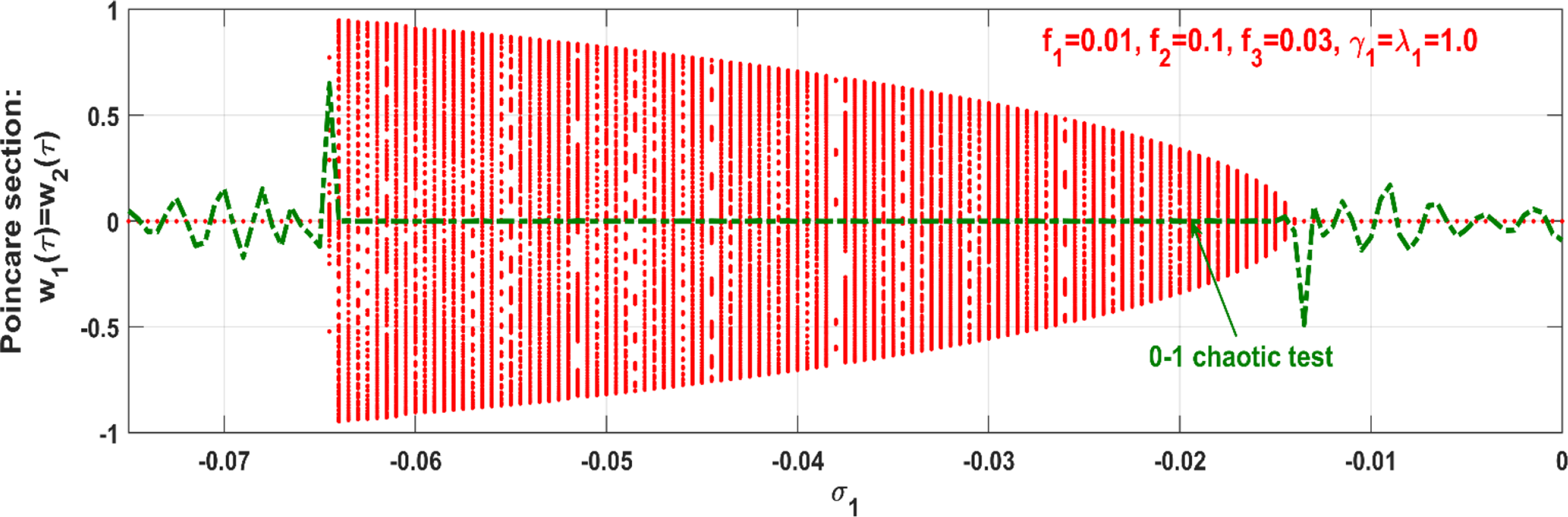
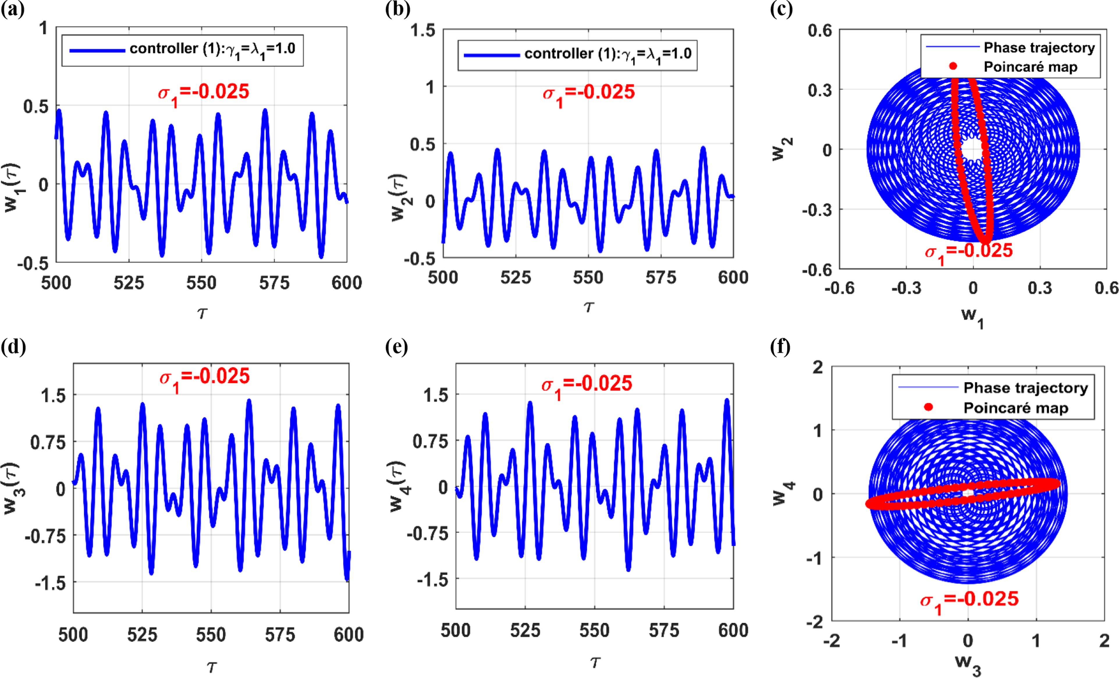
The angular velocity interval $-0.065\le {\sigma }_1\le -0.015$ , identified analytically in the close-up views of Figures 13(a) and 13(b), indicates that the rotor may exhibit unstable periodic motion. To further investigate this, a bifurcation diagram was established by numerically integrating equations (11.1)–(11.4). The Poincaré section on the plane $w_1\left(\tau \right)=w_2\left(\tau \right)$ was plotted against $\mathrm{\Omega }=1+{\sigma }_1$ over the interval $-0.075\le {\sigma }_1\le 0.0$ , as shown in Figure 14. Additionally, the $0–1$ chaos test was conducted for the system’s steady-state oscillations across this interval.^62,63 The figure demonstrates that the two-pole rotor system, under the influence of the $PPFC$ , transitions from periodic to quasiperiodic motion in the angular speed range $\mathrm{\Omega }=1+{\sigma }_1,-0.065\le {\sigma }_1\le -0.015$ , which closely aligns with the analytical results in Figure 13.

Figure 14.

Bifurcation diagram of the two-pole rotor model under $PPFC$ established according to Figure 13 on the interval $-0.075\le {\sigma }_1\le 0$ .

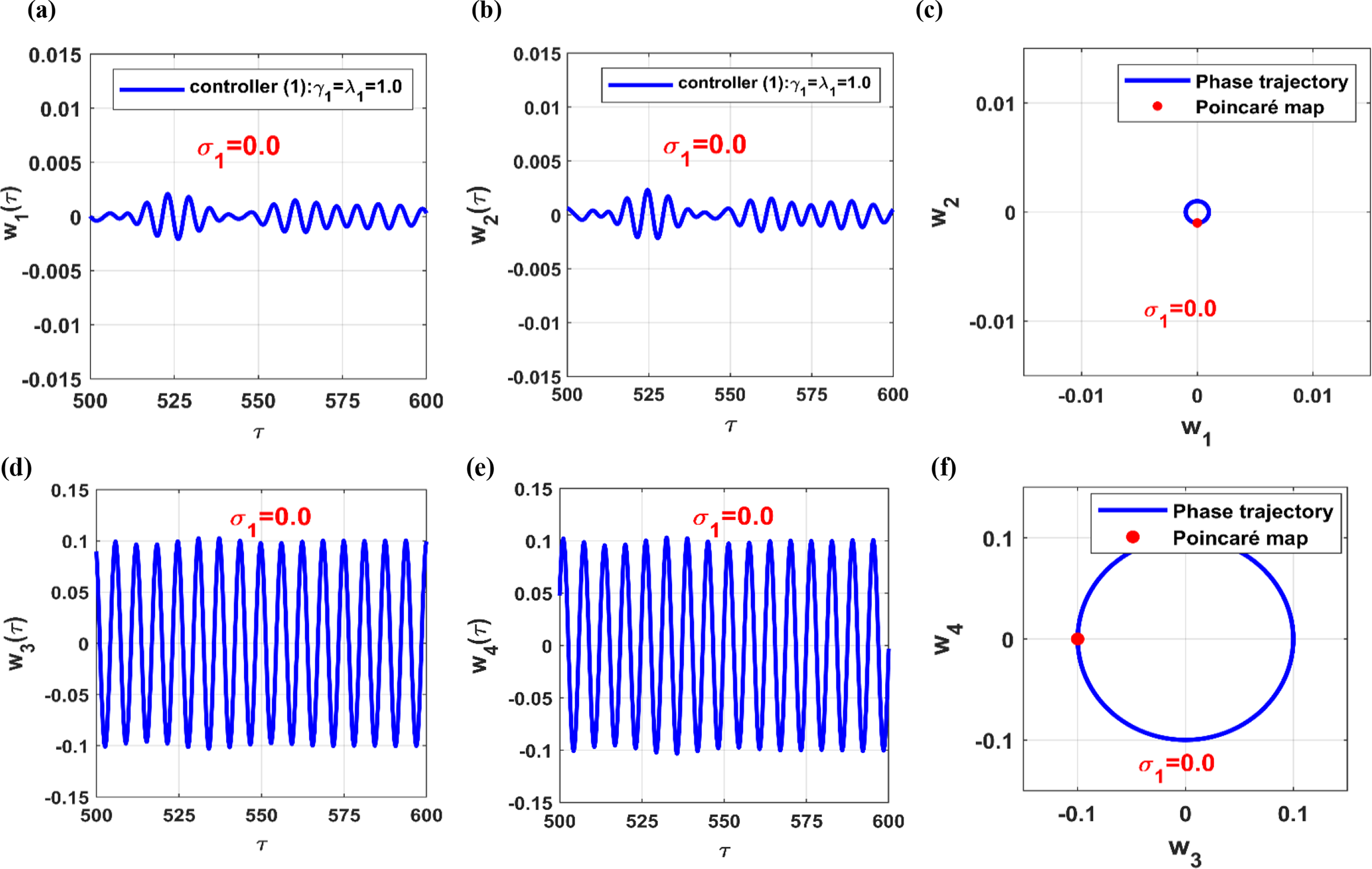
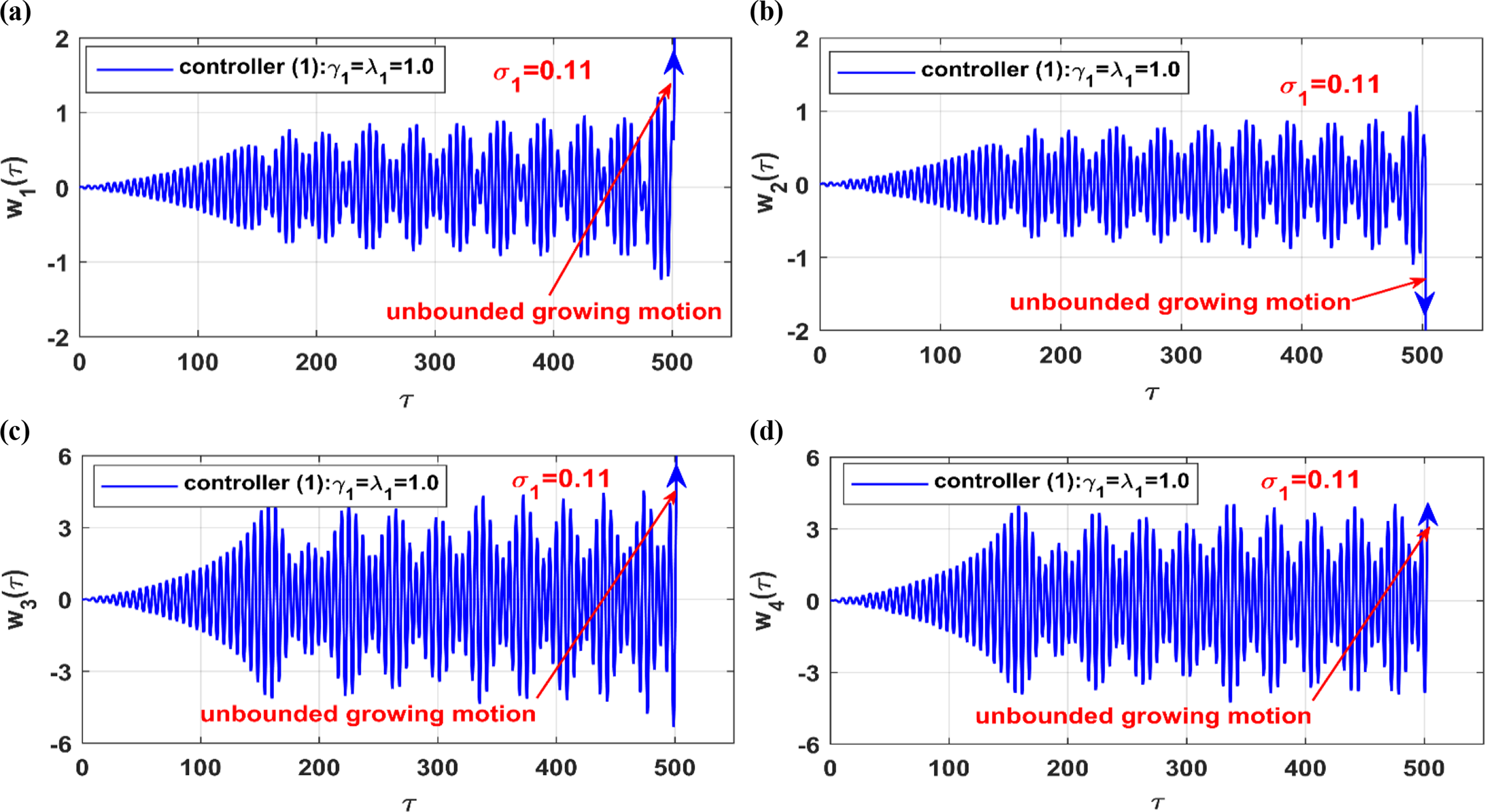
To further visualize the temporal oscillation amplitudes of both the two-pole system and the coupled $PPFC$ in the stable and unstable regions reported in Figures 13 and 14, equations (11.1)–(11.4) were numerically simulated for ${\sigma }_1=-0.025$ (an unstable point in Figures 13 and 14) and ${\sigma }_1=0.0$ (a stable point). Figures 15 and 16 present the results: Figure 15 shows quasiperiodic oscillations at ${\sigma }_1=-0.025$ , while Figure 16 demonstrates small-amplitude periodic motion at ${\sigma }_1=0.0$ . In Figure 17, the temporal oscillations of the two-pole system and the $PPFC$ at ${\sigma }_1=0.11$ (an unstable point in Figure 13) are simulated, revealing growing unbounded oscillations, which confirm the instability of the closed-loop system at $\mathrm{\Omega }=1+0.11$ . Based on Figures 13–17, it can be concluded that the analytical solution in Figure 13 and the numerical simulations in Figure 14–17 are in strong agreement. However, while coupling the $PPFC$ to the two-pole system effectively eliminates resonant vibrations (i.e., at ${\sigma }_1=0.0$ ), it introduces destabilizing effects, leading to either quasiperiodic or unbounded vibrations in the closed-loop system at certain angular velocities.

Figure 15.

Quasiperiodic oscillation of the two-pole rotor model and the coupled $PPFC$ according to the bifurcation diagram in Figure 14 when ${\sigma }_1=-0.025$ .

Figure 16.

Periodic oscillation of the two-pole rotor model and the coupled $PPFC$ according to the bifurcation diagram in Figure 14 when ${\sigma }_1=0.0$ .

Figure 17.

Unbounded growing oscillation of the two-pole rotor model and the coupled $PPFC$ according to the bifurcation diagram in Figure 13 when ${\sigma }_1=0.11$ .

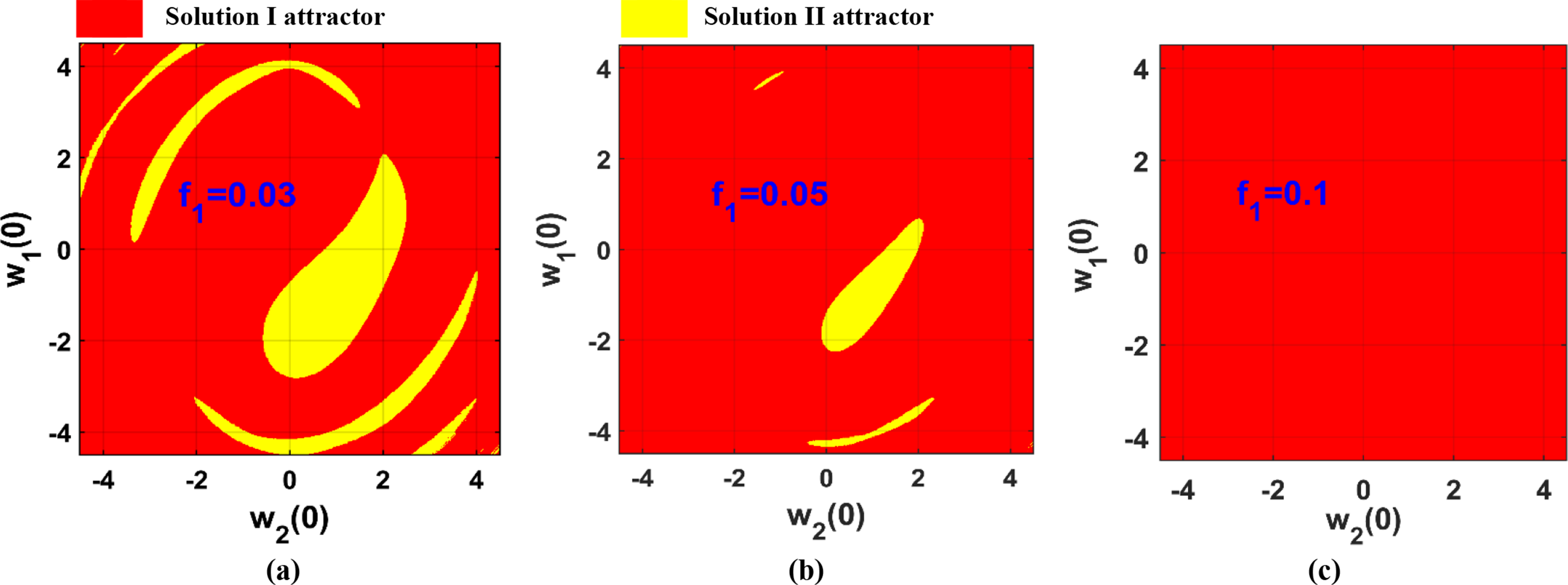
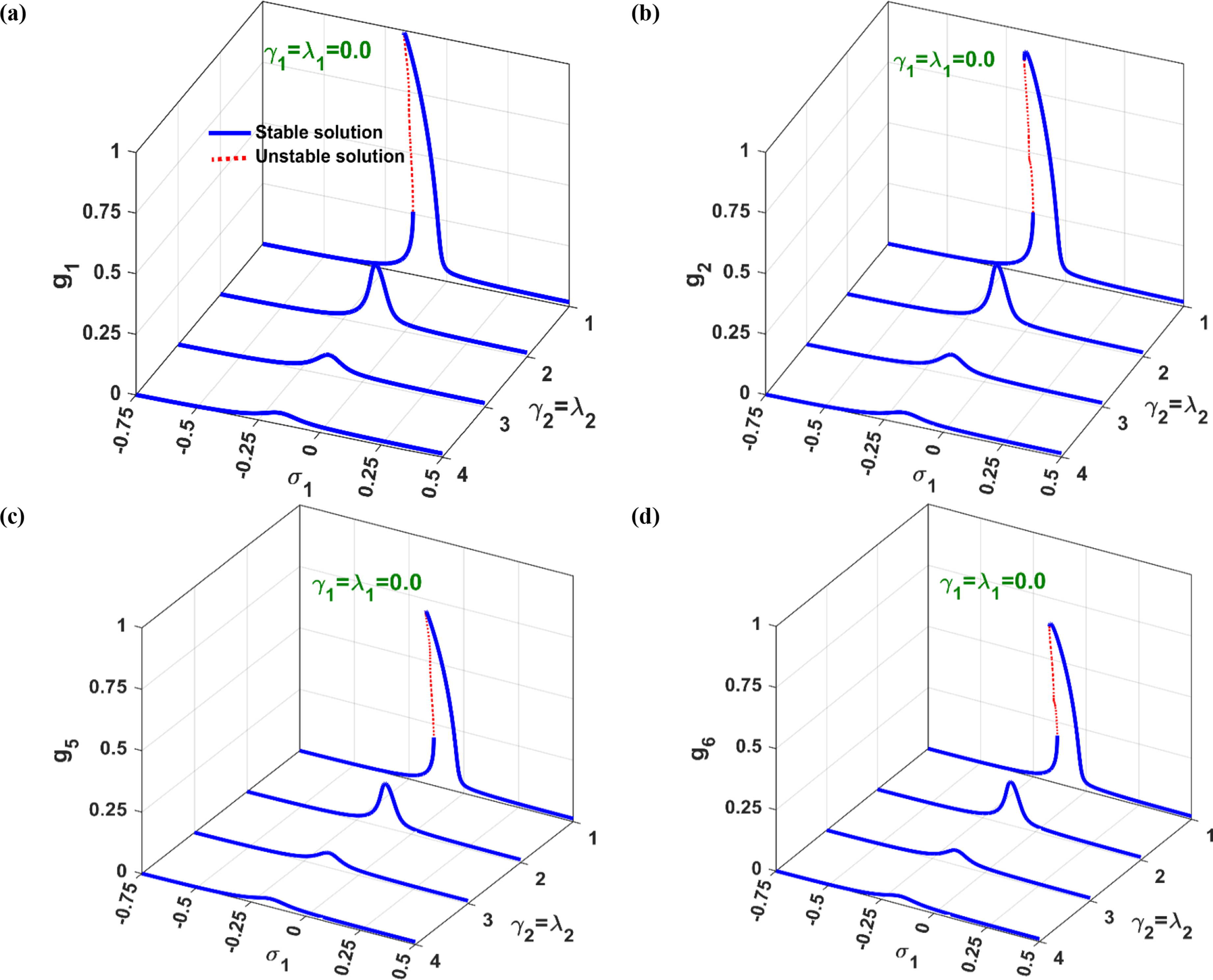
In Figure 18, the evolution of $g_1$ , $g_2$ , $g_3,$ and $g_4$ is plotted against ${\sigma }_1$ for four different values of the $PPFC$ control gain ( ${\gamma }_1={\lambda }_1=1.0,2.0,3.0,$ and $4.0$ ). The figure shows that increasing the gain widens the angular speed range around ${\sigma }_1=0.0$ where the rotor experiences small vibration amplitudes. However, increasing ${\gamma }_1={\lambda }_1$ from $1.0$ in Figure 13 to $4.0$ in Figure 18 does not stabilize the system within the interval $-0.065\le {\sigma }_1\le -0.015$ as reported in Figure 13. From the results presented in Figure 13–18, it can be concluded that the $PPFC$ fails to suppress the multistability behavior of the system. In fact, it may destabilize the stable motion of the uncontrolled model close to the resonant condition.

Figure 18.

Evolution of $g_1,$ $g_2,g_3$ , and $g_4$ of the two-pole rotor model and the coupled $PPFC$ (i.e., controller-1) against ${\sigma }_1$ when ${\gamma }_1={\lambda }_1=1.0,2.0,3.0,$ $4.0$ , and ${\gamma }_2={\lambda }_2=0.0$ .

Rotor dynamics under controller-2: IRC

In this subsection, the bifurcation characteristics of the two-pole system subjected to simultaneous external ( $f_1$ ), linear parametric ( $f_2$ ), and nonlinear parameter ( $f_3$ ) excitations are explored under the action of the $IRC$ only. Coupling the $IRC$ to the system means that the control currents, given by equations (7.1) and (7.2), are reduced to $I_x=-k_{12}{v}_1\left(t\right)$ and $I_y=-k_{22}{v}_2\left(t\right)$ , while $k_{11}=k_{21}=0.0$ . Additionally, the normalized equations governing the system dynamics, with the $IRC$ , reduce to equations (11.1), (11.2), (11.5), and (11.6), where the dimensionless control gains for the $IRC$ are ${\gamma }_2=h{k}_{12}/I_b$ and ${\lambda }_2=h{k}_{22}/I_b$ . Accordingly, the evolution of the system’s and $IR{C}^{\prime }s$ oscillation amplitudes (i.e., $g_1,g_2,g_5,$ and $g_6$ ) is investigated in terms of the control gains ${\gamma }_2$ and ${\lambda }_2$ .

In Figure 19, the evolution of $g_1,{\hspace{0.17em}g}_2,g_5,$ and $g_6$ is plotted against ${\sigma }_1$ with the normalized $IRC$ control gains set to ${\gamma }_2={\lambda }_2=1.0$ . The figure clearly shows that integrating the $IRC$ into the two-pole system significantly improves the complex bifurcation characteristics of the uncontrolled model shown in Figure 3. Tri-stability characteristics and the existence of isolated solution branches are eliminated. Furthermore, a comparison of Figures 13 and 19 reveals that the $IRC$ is more effective than the $PPFC$ for the same control signal gains (i.e., ${\gamma }_1={\lambda }_1={\gamma }_2={\lambda }_2=1.0$ ). The rotor motion remains stable along the ${\sigma }_1$ axis, regardless of angular velocity, as shown in Figure 19, whereas the response curve in Figure 13 is more complex. Moreover, the $IRC$ introduces only one resonant peak near ${\sigma }_1=0.0$ , attributed to its damping effect, compared to the $PPFC$ .

Figure 19.

Evolution of $g_1,$ $g_2,g_5$ , and $g_6$ of the two-pole rotor model and the coupled $IRC$ (i.e., controller-2) against ${\sigma }_1$ when ${\gamma }_1={\lambda }_1=0.0$ , and ${\gamma }_2={\lambda }_2=1.0$ .

Figure 20 visualizes the evolution of $g_1,{\hspace{0.17em}g}_2,g_5,$ and $g_6$ against ${\sigma }_1$ under four different $IRC$ control gains ${\gamma }_2={\lambda }_2$ . The figure demonstrates that the resonant peaks of both the controlled two-pole rotor system and the coupled $IRC$ decrease monotonically with increasing control gain ${\gamma }_2={\lambda }_2$ . The bi-stable solution observed in Figure 19 at ${\gamma }_2={\lambda }_2=1.0$ disappears when the $IRC$ gain is increased to ${\gamma }_2={\lambda }_2=2.0$ . Additionally, the figure shows that not only can the complex bifurcation characteristics reported in Figure 3 be controlled using the $IRC$ control gains, but also that system vibrations can be reduced to very small levels at higher control gains (i.e., ${\gamma }_2={\lambda }_2=4.0$ ). By comparing the steady-state oscillatory behavior of the controlled two-pole rotor system under both the $PPFC$ and $IRC$ , as shown in Figures 18 and 20, one can infer the superiority of the $IRC$ in stabilizing the system and mitigating undesired oscillations compared to the $PPFC$ .

Figure 20.

Evolution of $g_1,$ $g_2,g_5$ , and $g_6$ of the two-pole rotor model and the coupled $IRC$ (i.e., controller-2) against ${\sigma }_1$ when ${\gamma }_1={\lambda }_1=0.0$ , and ${\gamma }_2={\lambda }_2=1.0,2.0,3.0,$ $4.0$ .

Rotor dynamics under controller-3: PPFC + IRC

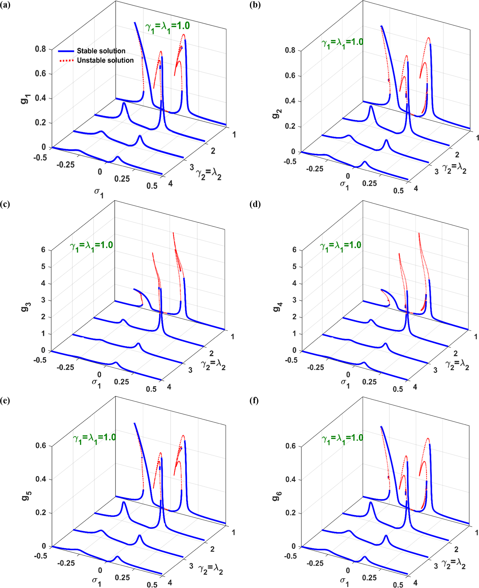
It is well known that the primary function of the $PPFC$ is to establish an energy bridge between the controlled system and the coupled controller, allowing the excess vibrational energy in the system to be transferred to the $PPFC$ through this bridge. In contrast, the vibration control mechanism of the $IRC$ involves controlling the magnitude of the system’s linear damping via the feedback and control gains of the $IRC$ ⁴³ . In this subsection, the bifurcation behavior of the two-pole rotor model, controlled by the $PPFC+IRC$ and subjected to simultaneous external ( $f_1$ ), linear parametric ( $f_2$ ), and nonlinear parameter ( $f_3$ ) excitations, is explored, as shown in Figure 21. Integrating the $PPFC+IRC$ into the two-pole rotor model involves applying the full control current given by equations (7.1) and (7.2), such that $I_x=-k_{11}{u}_1\left(t\right)-k_{12}{v}_1\left(t\right)$ and $I_y=-k_{21}{u}_2\left(t\right)-k_{22}{v}_2\left(t\right)$ , where the corresponding dimensionless control gains $k_{11},k_{12},k_{21}$ , and $k_{22}$ are defined as ${\gamma }_1=h{k}_{11}/I_b,{\gamma }_2=h{k}_{12}/I_b,{\lambda }_1=h{k}_{21}/I_b,$ and ${\lambda }_2=h{k}_{22}/I_b$ . Additionally, the coupled normalized equations governing the dynamics of the rotor, $PPFC,$ and $IRC$ are given by equations (11.1)–(11.6).

Figure 21.

Evolution of $g_1,$ $g_2,g_3,g_4,g_5$ , and $g_6$ of the two-pole rotor model and the coupled $IRC+PPFC$ (i.e., controller-3) against ${\sigma }_1$ when ${\gamma }_1={\lambda }_1=1.0$ and ${\gamma }_2={\lambda }_2=1.0,2.0,3.0,4.0$ .

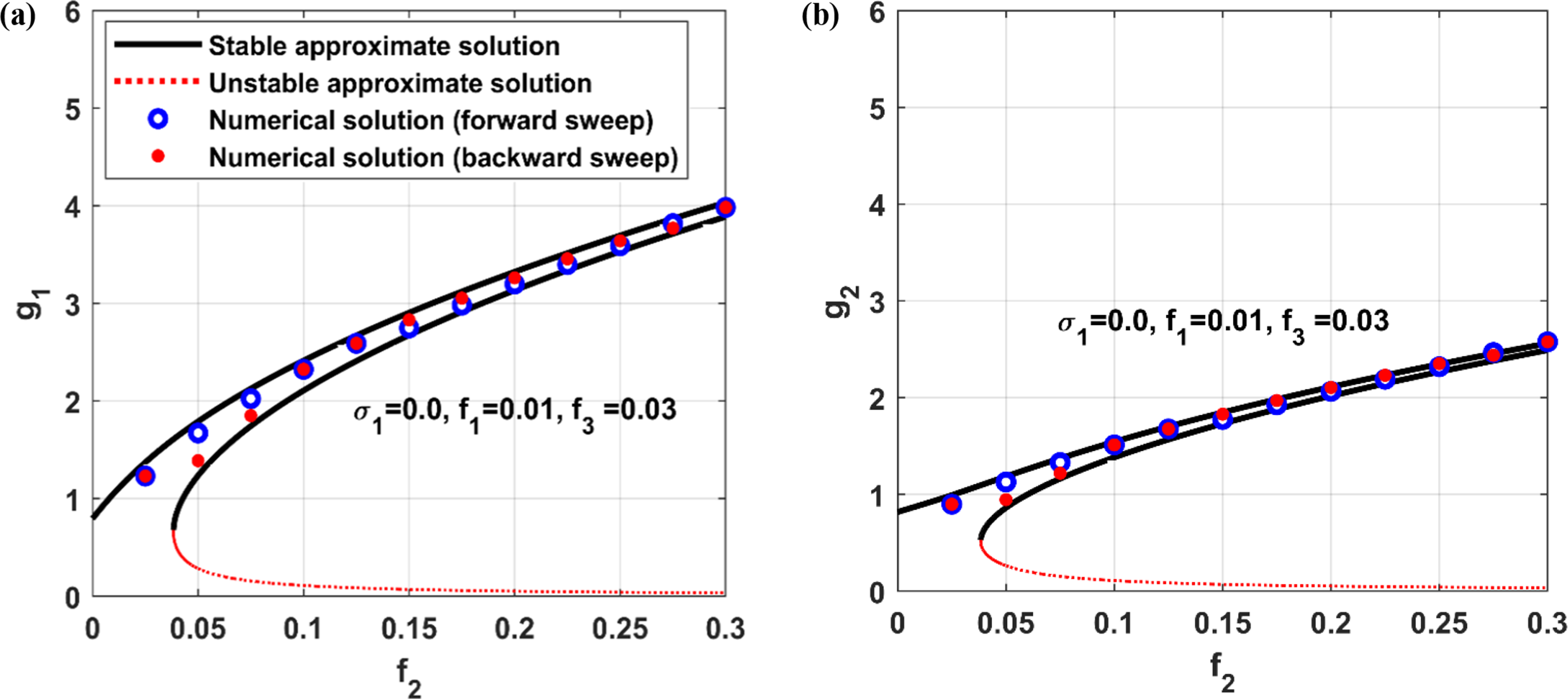
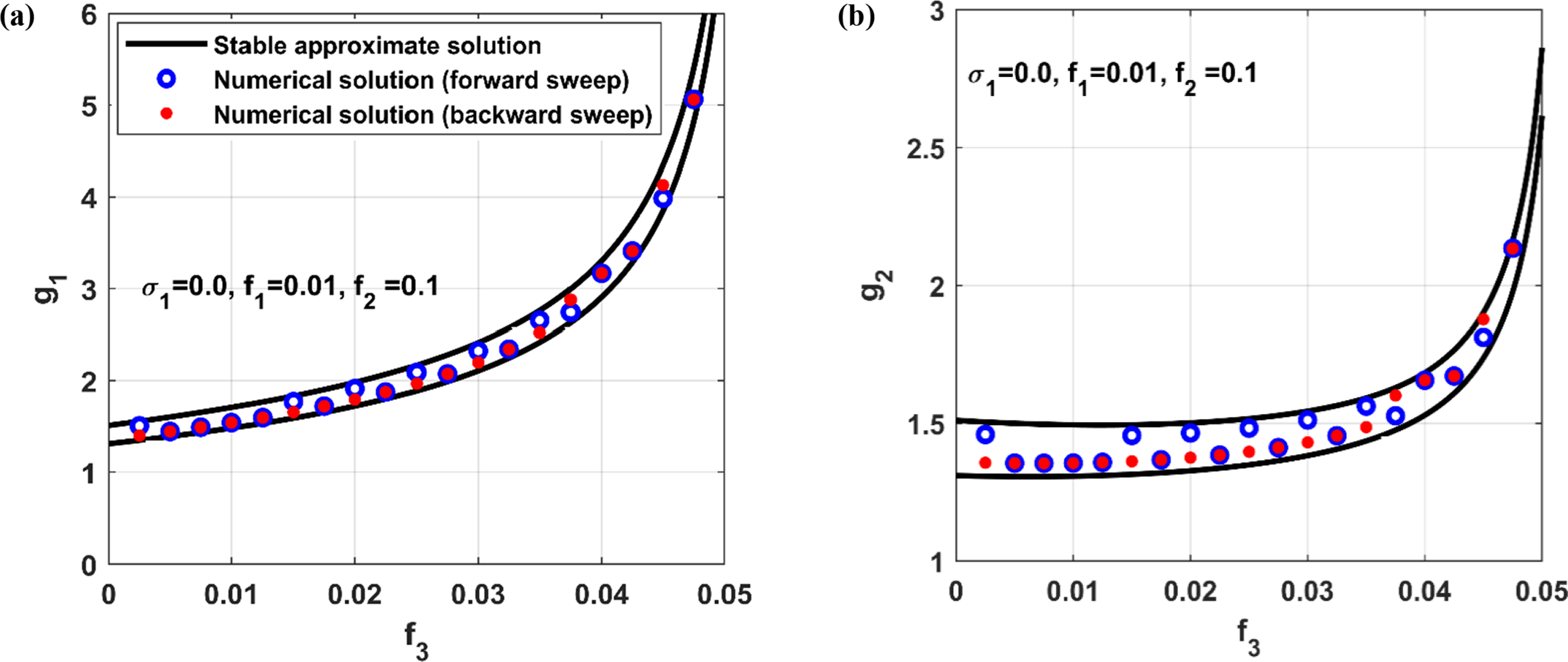
To explore the steady-state evolution of the rotor, $PPFC$ , and $IRC$ vibration amplitudes $g_1,{\hspace{0.17em}g}_2,g_3,g_4,{\hspace{0.17em}g}_5,$ and $g_6$ , the nonlinear system described by equations (23.1)–(23.8) must be solved, taking into account the definition $g_5={\delta }_1{g}_1/\sqrt{{\delta }_1^2+1}$ and $g_6={\delta }_2{g}_2/\sqrt{{\delta }_2^2+1}$ , as defined below equation (22.6). Figure 21 presents the evolution of $g_1,{\hspace{0.17em}g}_2,g_3,g_4,{\hspace{0.17em}g}_5,$ and $g_6$ against ${\sigma }_1$ with ${\gamma }_1={\lambda }_1=1.0$ for ${\gamma }_2={\lambda }_2=1.0,2.0,3.0,$ and $4.0$ . Comparing Figure 21 with Figure 13, it is evident that increasing the control gain ${\gamma }_2={\lambda }_2$ from $1.0$ to $4.0$ , while keeping ${\gamma }_1={\lambda }_1=1.0$ , improves the vibration reduction performance of the $PPFC+IRC$ (controller-3) and stabilizes the previously unstable solution reported in Figure 13.

Vibration suppression performance of controller-2 against controller-3

In this subsection, we evaluate the performance of controller-2 ( $IRC$ ) against controller-3 ( $PPFC+IRC$ ) under varying intensities of external, linear parametric, and nonlinear parametric excitations. The objective is to identify the optimal control approach for systems exposed to combined excitation forces, ensuring enhanced stability and reduced oscillation amplitudes. By contrast, Controller-1 ( $PPFC$ ) is ineffective in mitigating unwanted oscillations or stabilizing the system dynamics when exposed to simultaneous external and multi-parametric periodic excitations, it is excluded from further comparison.

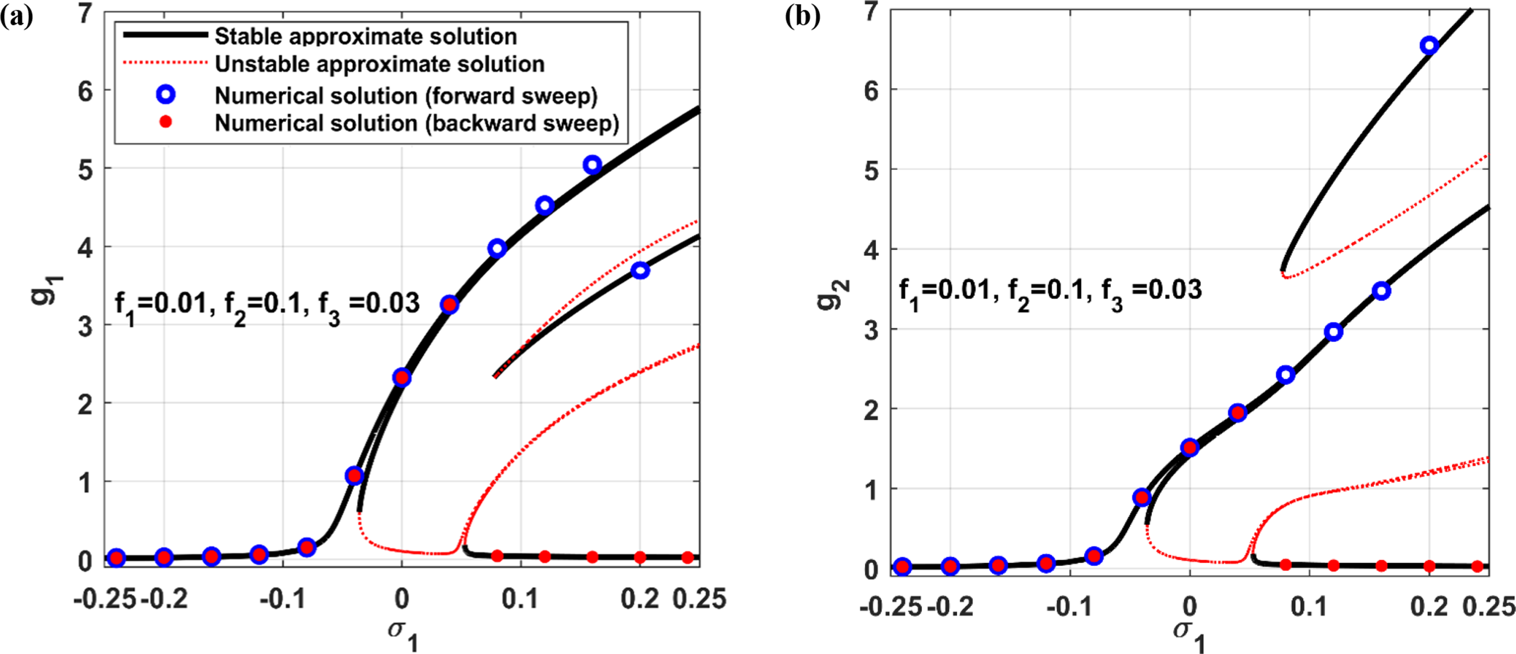
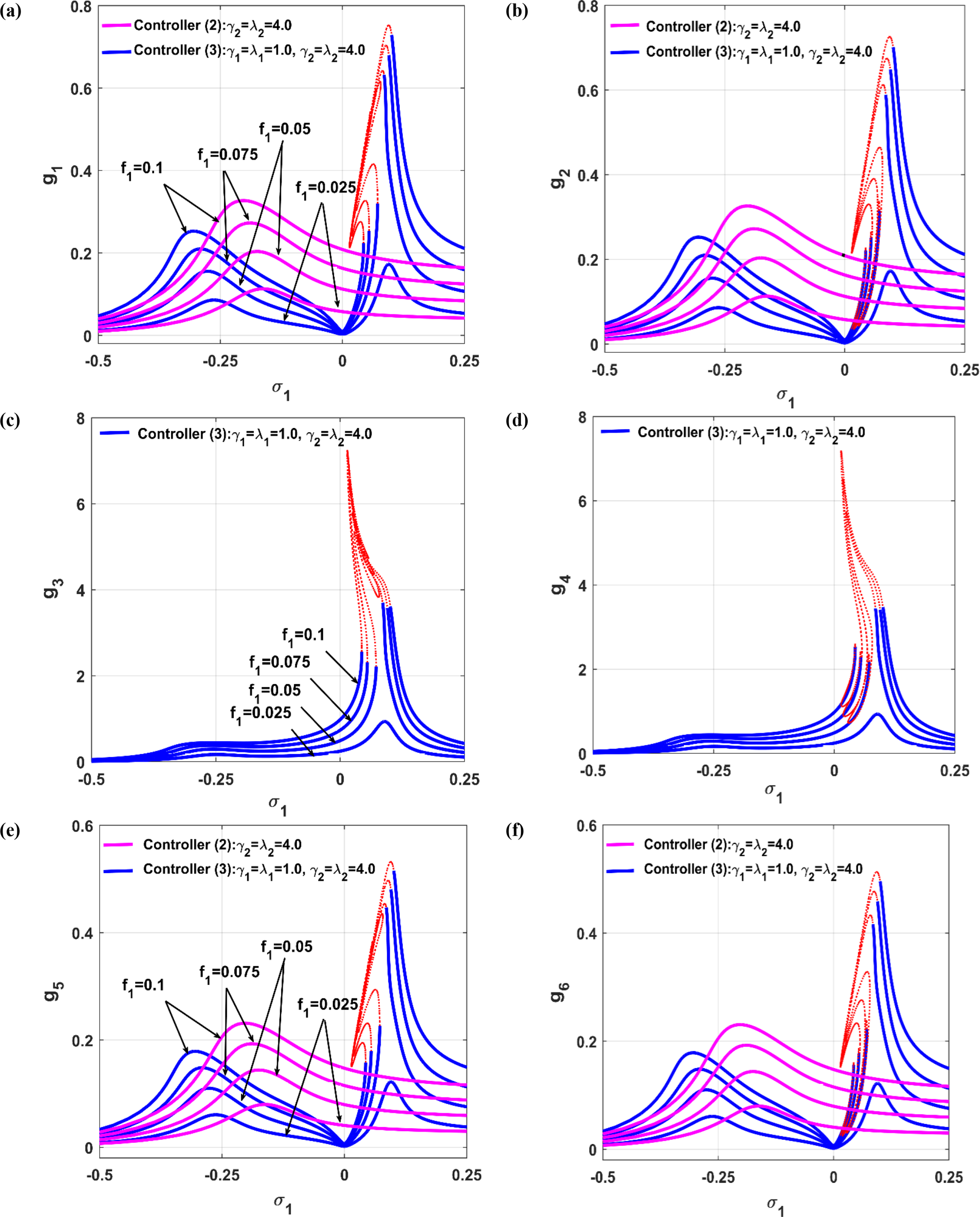
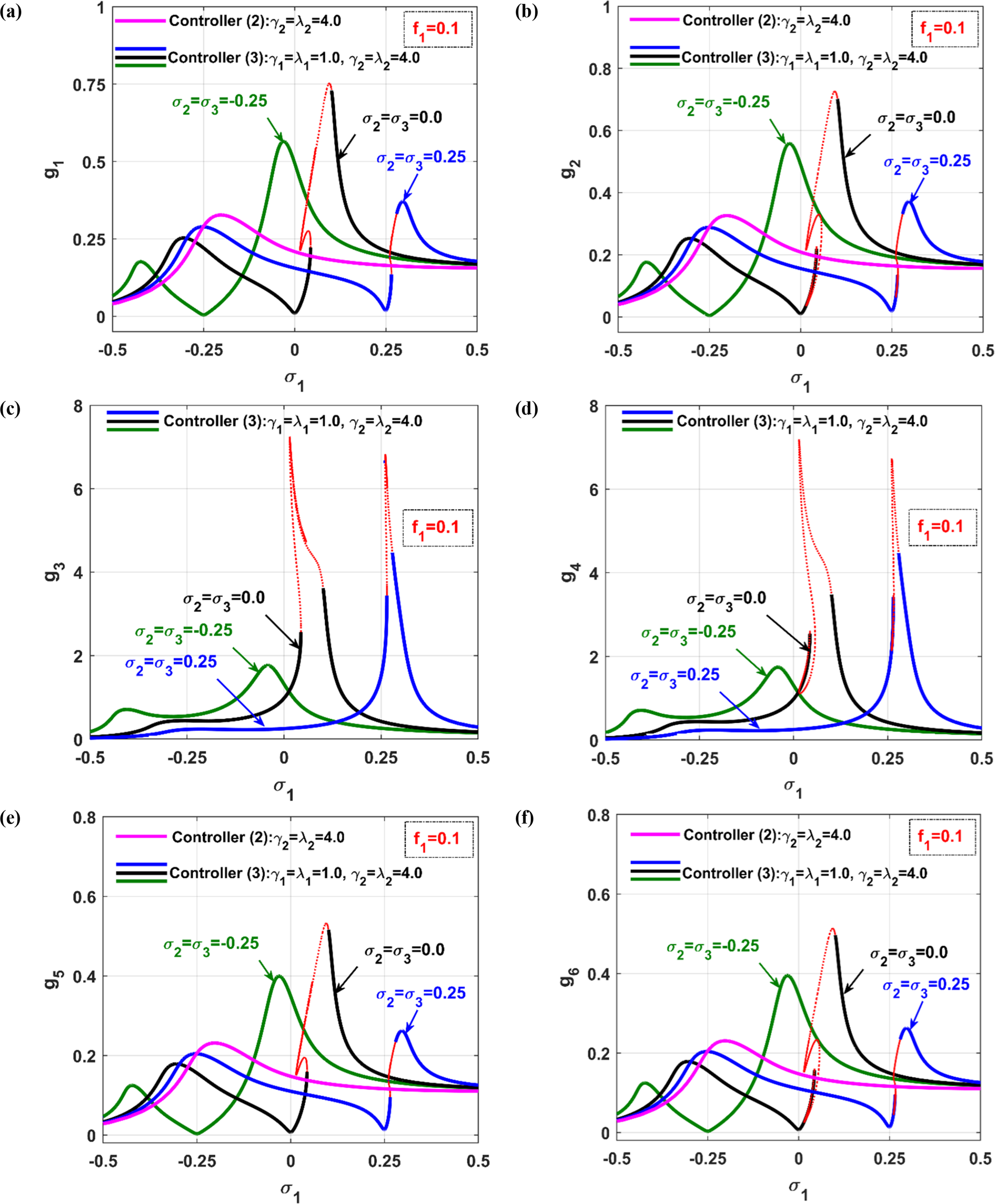
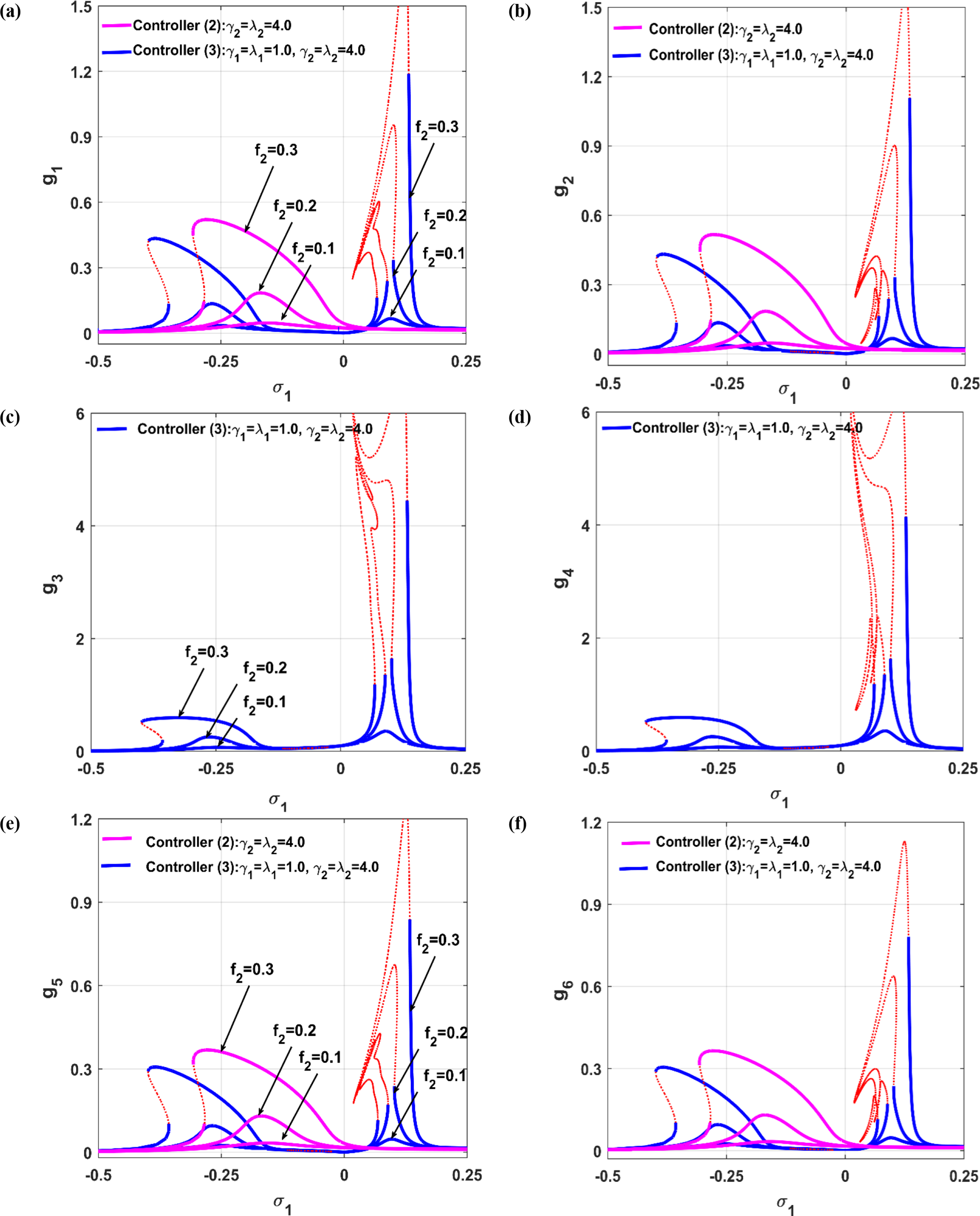
The control gains in the following analysis are set to ${\gamma }_1={\lambda }_1=1.0$ and ${\gamma }_2={\lambda }_2=4.0$ . In Figure 22, the evolution of $g_1,{\hspace{0.17em}g}_2,g_3,g_4,{\hspace{0.17em}g}_5,$ and $g_6$ is plotted against ${\sigma }_1$ under the action of both controller-2 and controller-3 at four different magnitudes of the external excitation force $f_1$ , while the other forces are kept constant at $f_2=0.1$ and $f_3=0.03$ . The figure indicates that the rotor vibration amplitudes $g_1$ and $g_2$ generally increase monotonically with $f_1$ in both cases of controller-2 and controller-3. However, the two-pole rotor response under controller-2 remains almost stable and linear, regardless of both the angular velocity and the external excitation force, which is not the case under controller-3. Under controller-3, the two-pole system may exhibit unstable behavior when ${\sigma }_1>0.0$ (i.e., when the angular velocity is higher than the first critical speed). However, the most significant result regarding controller-3 is its ability to maintain rotor oscillation close to zero in perfect resonance conditions (i.e., when ${\sigma }_1=0.0$ ) regardless of the magnitude of $f_1$ .

Figure 22.

Evolution of $g_1$ and $g_2$ under controller-2 and controller-3 at different levels of the external excitation force $f_1$ , while the parametric forces are fixed at $f_2=0.1$ and $f_3=0.03$ .

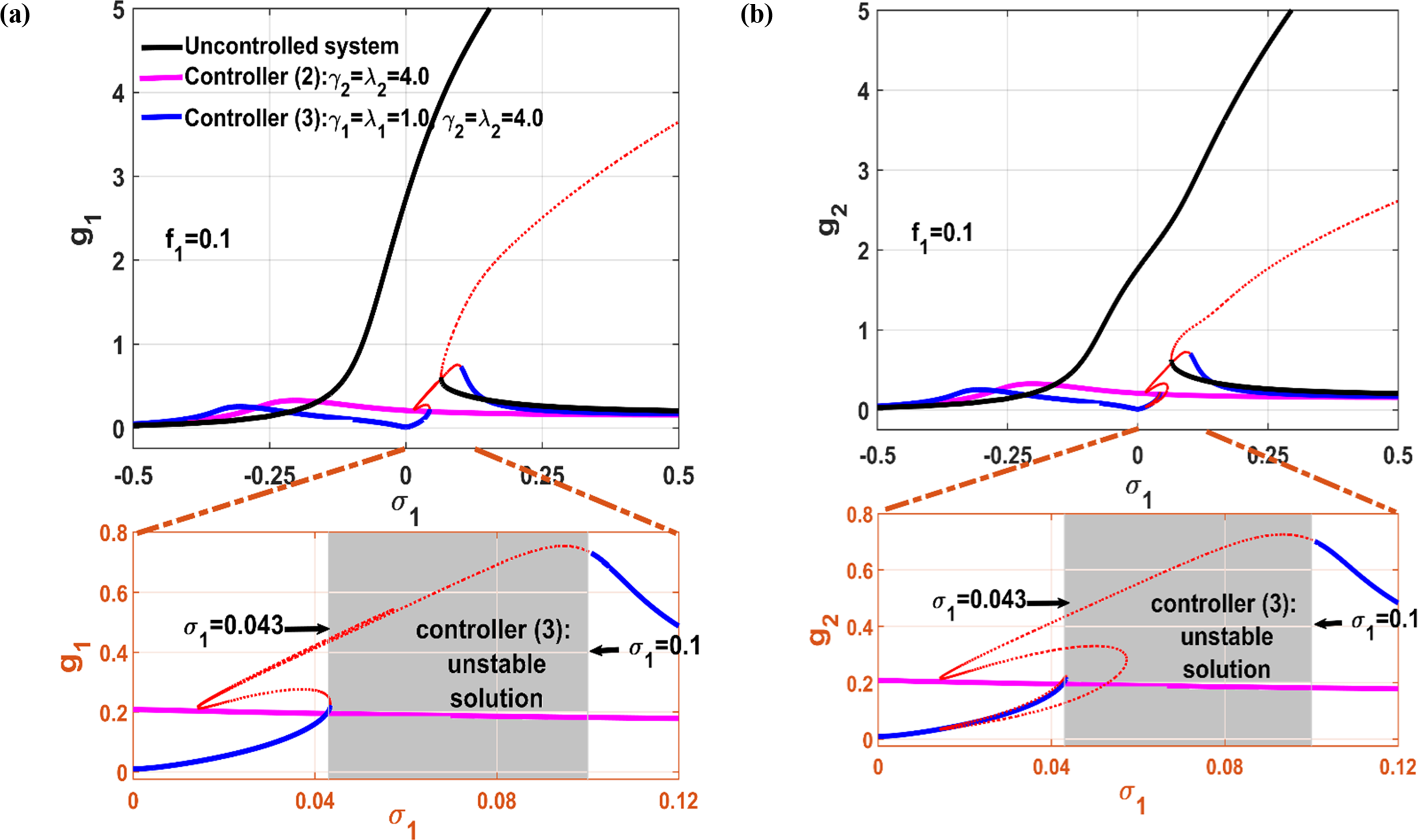
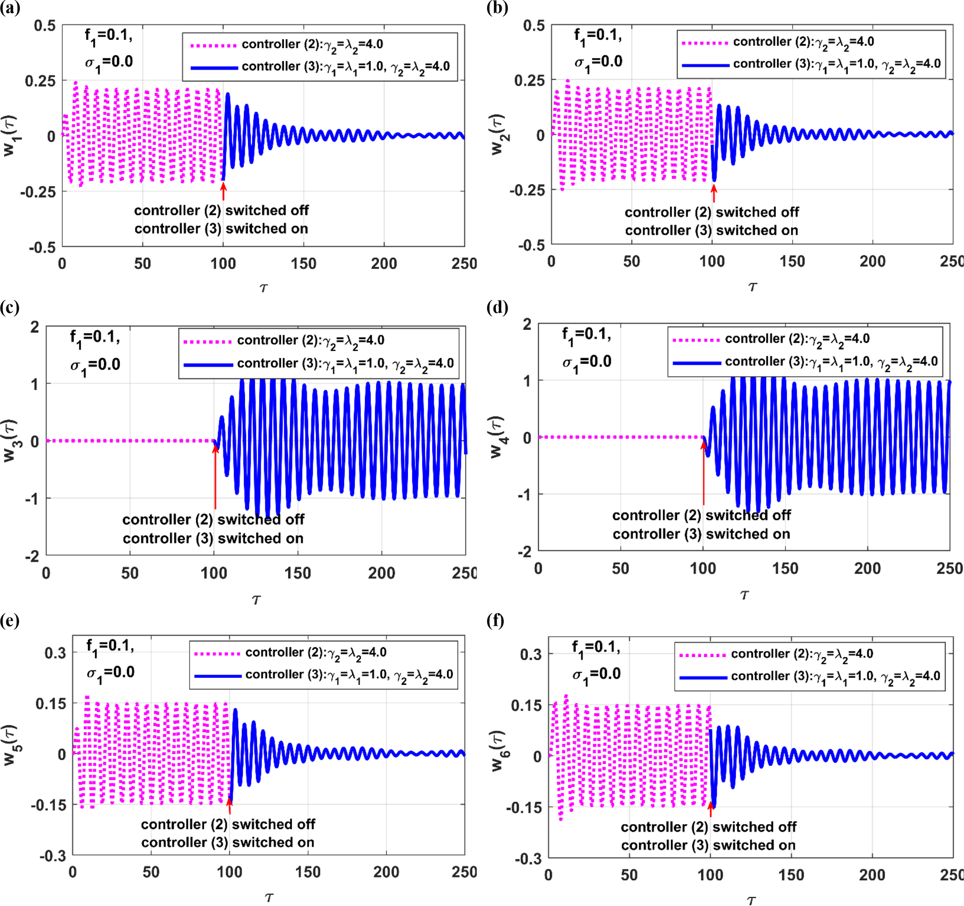
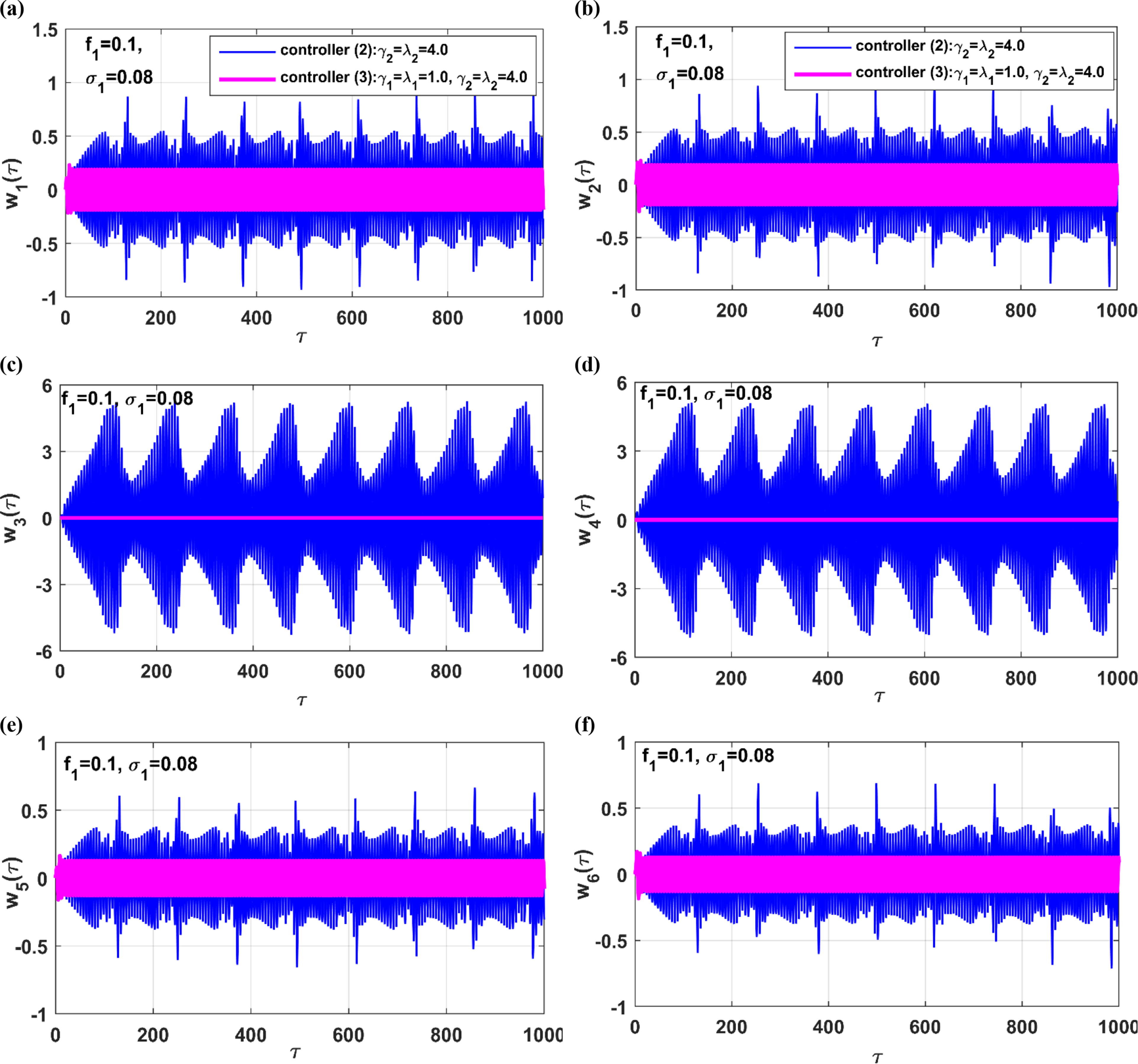
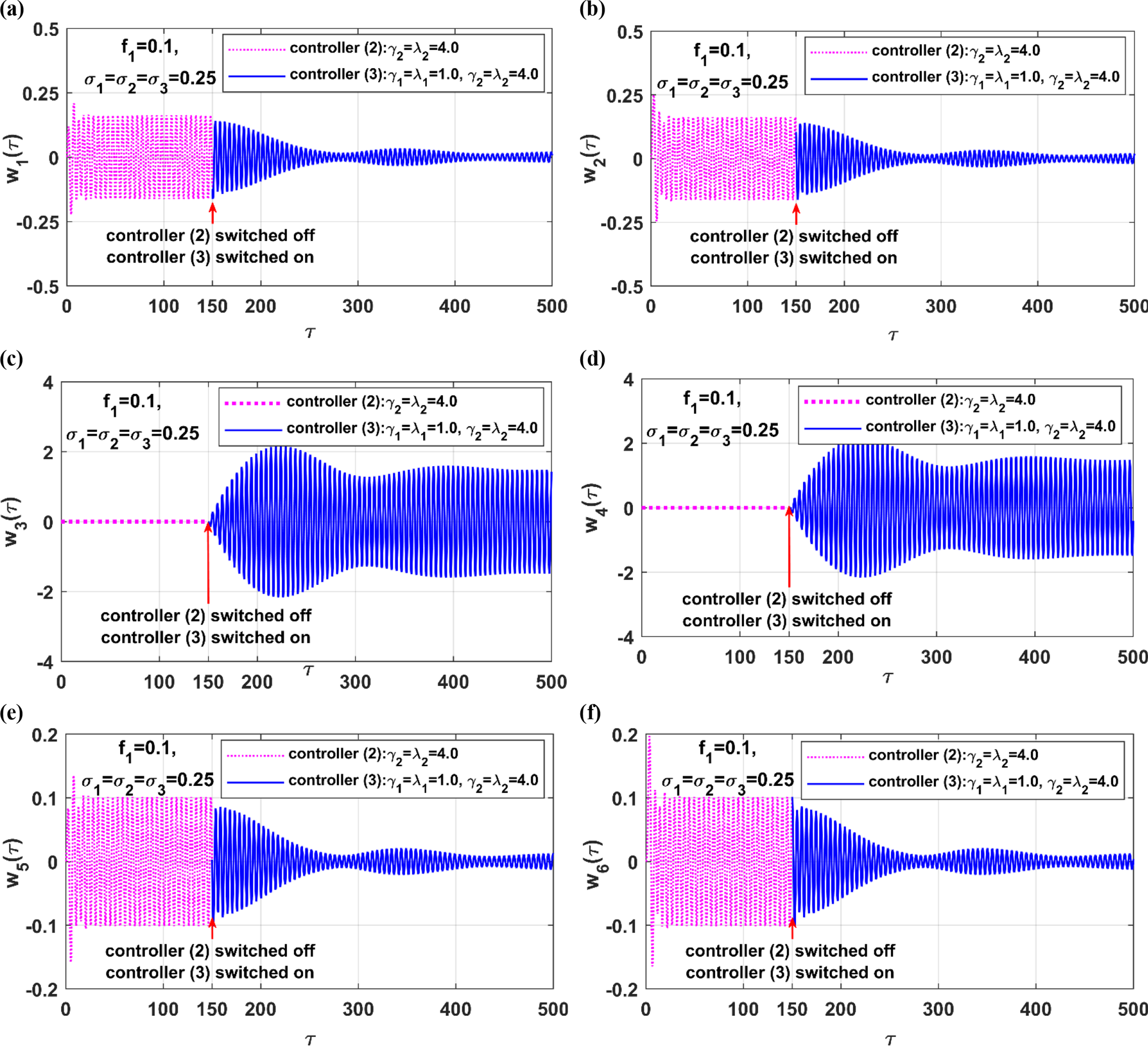
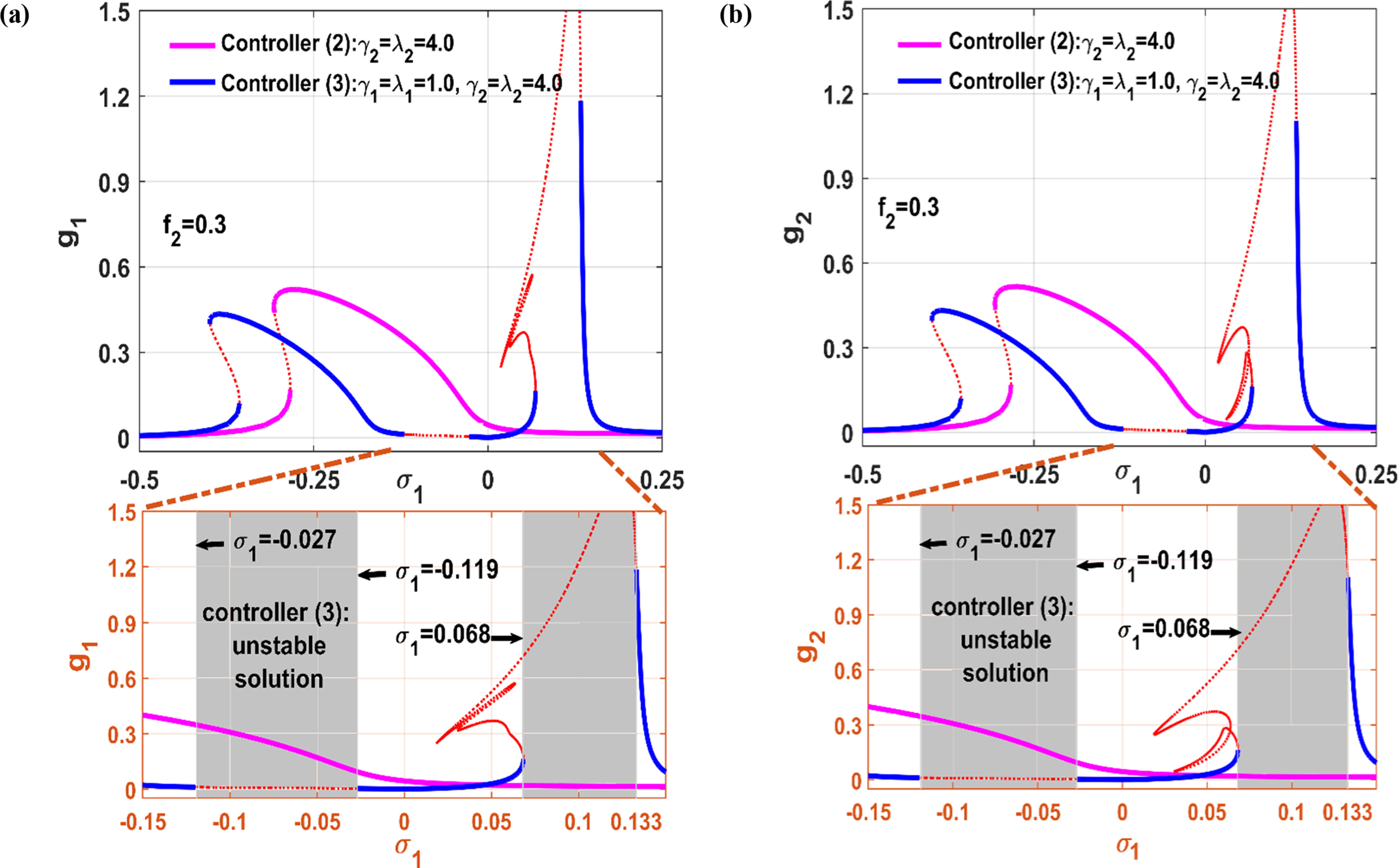
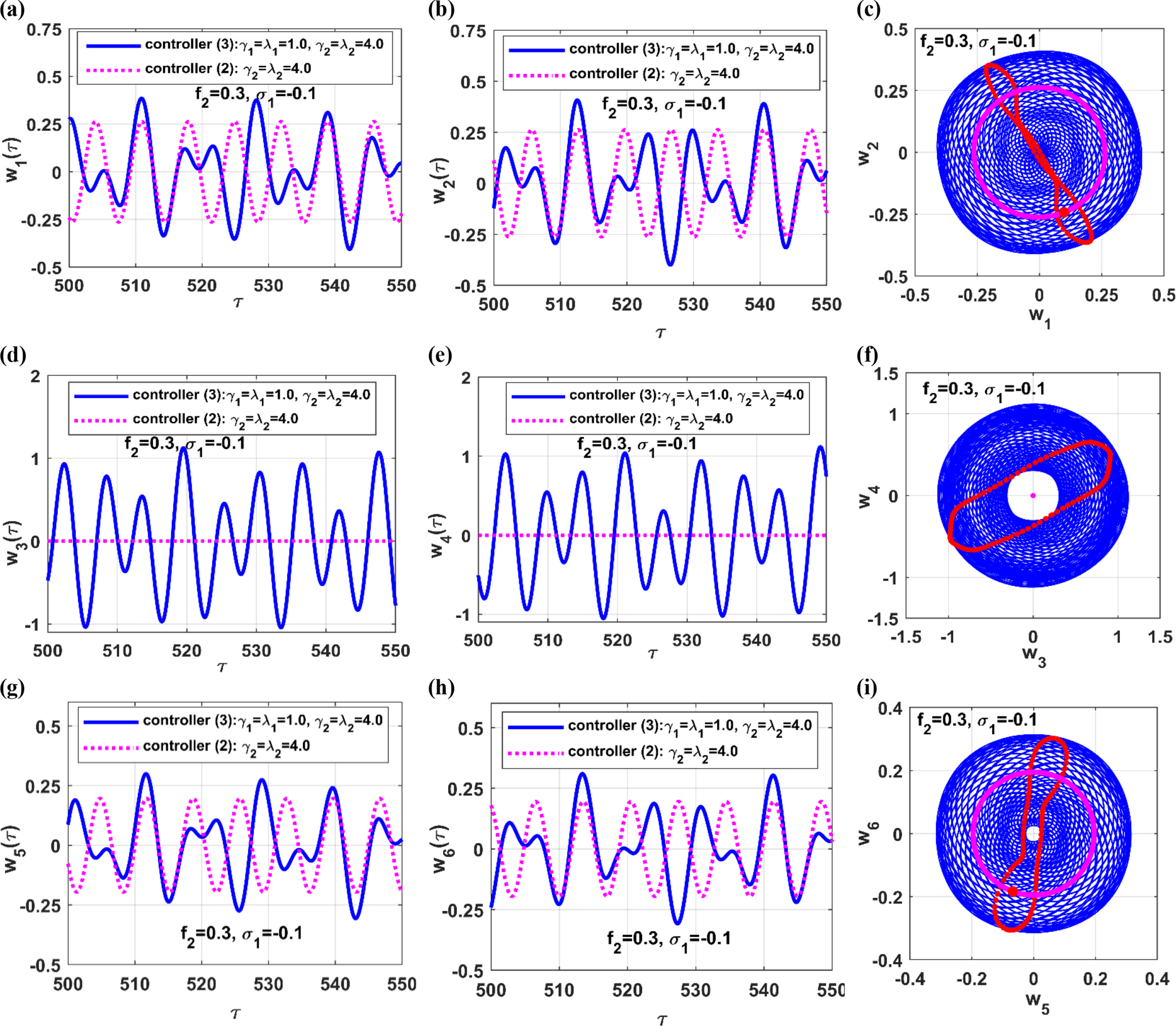
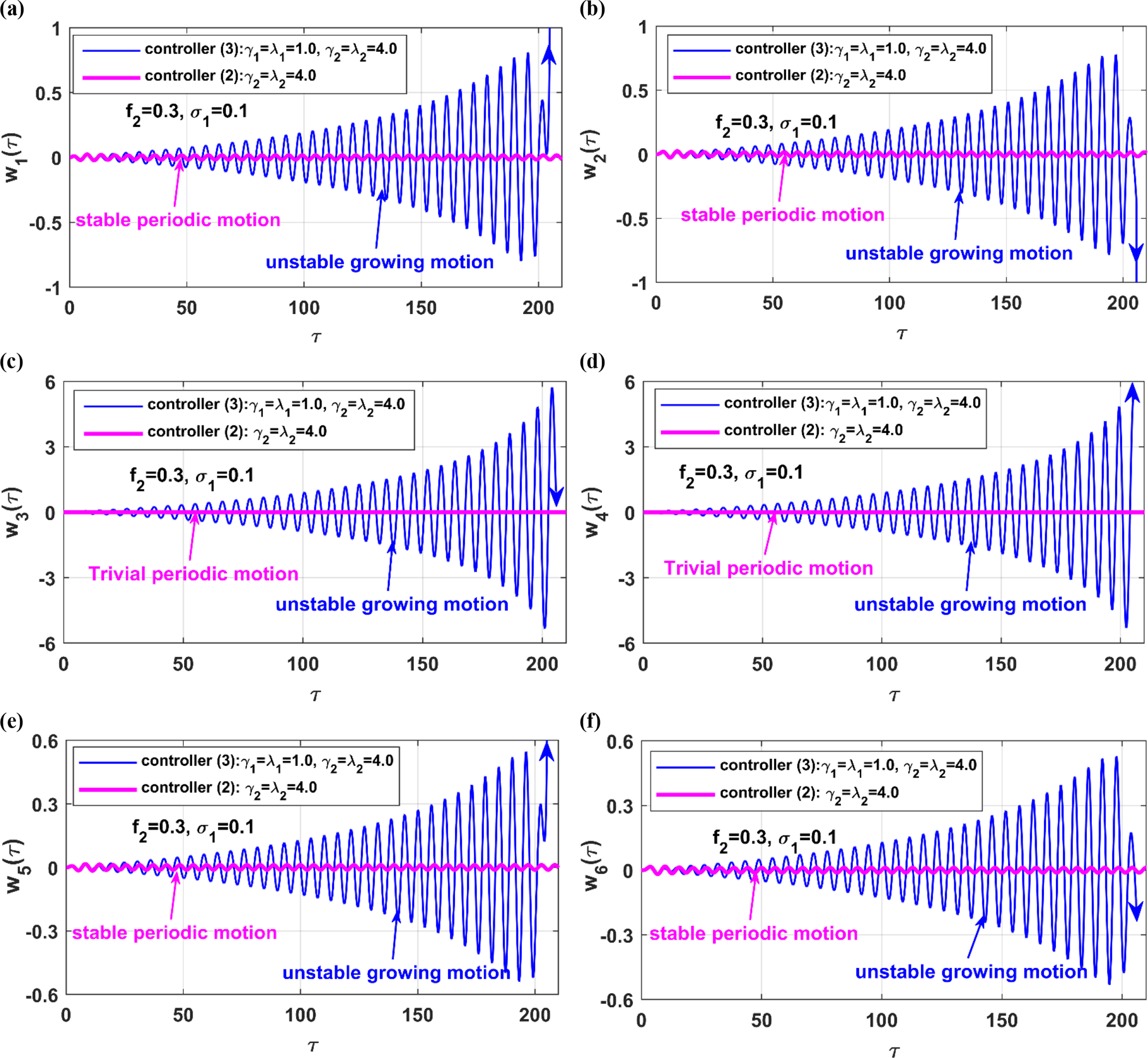
To demonstrate these phenomena numerically, a closer view of Figure 22, focusing on $g_1$ and $g_2$ when $f_1=0.1$ , is depicted in Figure 23. By examining the figure, one can first observe that the oscillation amplitudes $g_1$ and $g_2$ are nearly zero under the action of controller-3 when ${\sigma }_1=0.0$ (i.e., $\mathrm{\Omega }=1\leftarrow$ normalized natural frequency). However, they have a significant magnitude under the action of controller-2. The second observation is that the two-pole system may lose stability under controller-3 over the interval 0 ${0.043<\sigma }_1<0.1$ , while the system remains stable under controller-2. To verify the first observation from Figure 23, equations (11.1)–(11.6), were numerically integrated with $f_1=0.1,f_2=0.1,f_3=0.03,$ $\mathrm{\Omega }=1.0+{\sigma }_1$ , and ${\sigma }_1=0.0$ , under the action of controller-2 over the normalized time interval $0\le \tau \le 100$ . At $\tau =100$ , controller-2 is switched off, and controller-3 is activated over the time interval $100<\tau <250$ , as shown in Figure 24. The figure illustrates the elimination of system oscillations, bringing them close to zero as soon as controller-3 is activated at $\tau =100$ , which aligns with the behavior observed in Figure 23 at ${\sigma }_1=0.0$ . To confirm the instability of controller-3 over the interval ${0.043<\sigma }_1<0.1$ , as reported in Figure 23, equations (11.1)–(11.6) were numerically integrated with ${\sigma }_1=0.08$ under the action of both controller-2 and controller-3 over the time interval $0\le \tau \le 1000$ , as illustrated in Figure 25. The figure clearly shows quasi-periodic oscillations of the two-pole system when coupled to controller-3, while it exhibits periodic motion under controller-2.

Figure 23.

A closer view of Figures 22(a) and 22(b) when $f_1=0.1$ .

Figure 24.

Instantaneous temporal oscillations of the two-pole rotor model under controllers (2) and (3), based on the bifurcation diagram in Figure 23, with ${\sigma }_1=0.0$ : controller-2 is active and controller-3 is inactive during the time interval $0\le \tau <100$ , while controller-3 is active and controller-2 is deactivated during the time interval $100\le \tau <250$ .

Figure 25.

Instantaneous temporal oscillations of the two-pole rotor model under controller-2 and 3, based on the bifurcation diagram in Figure 23, with ${\sigma }_1=0.08$ : stable oscillations occur under controller-2, while quasiperiodic oscillations are observed under controller-3.

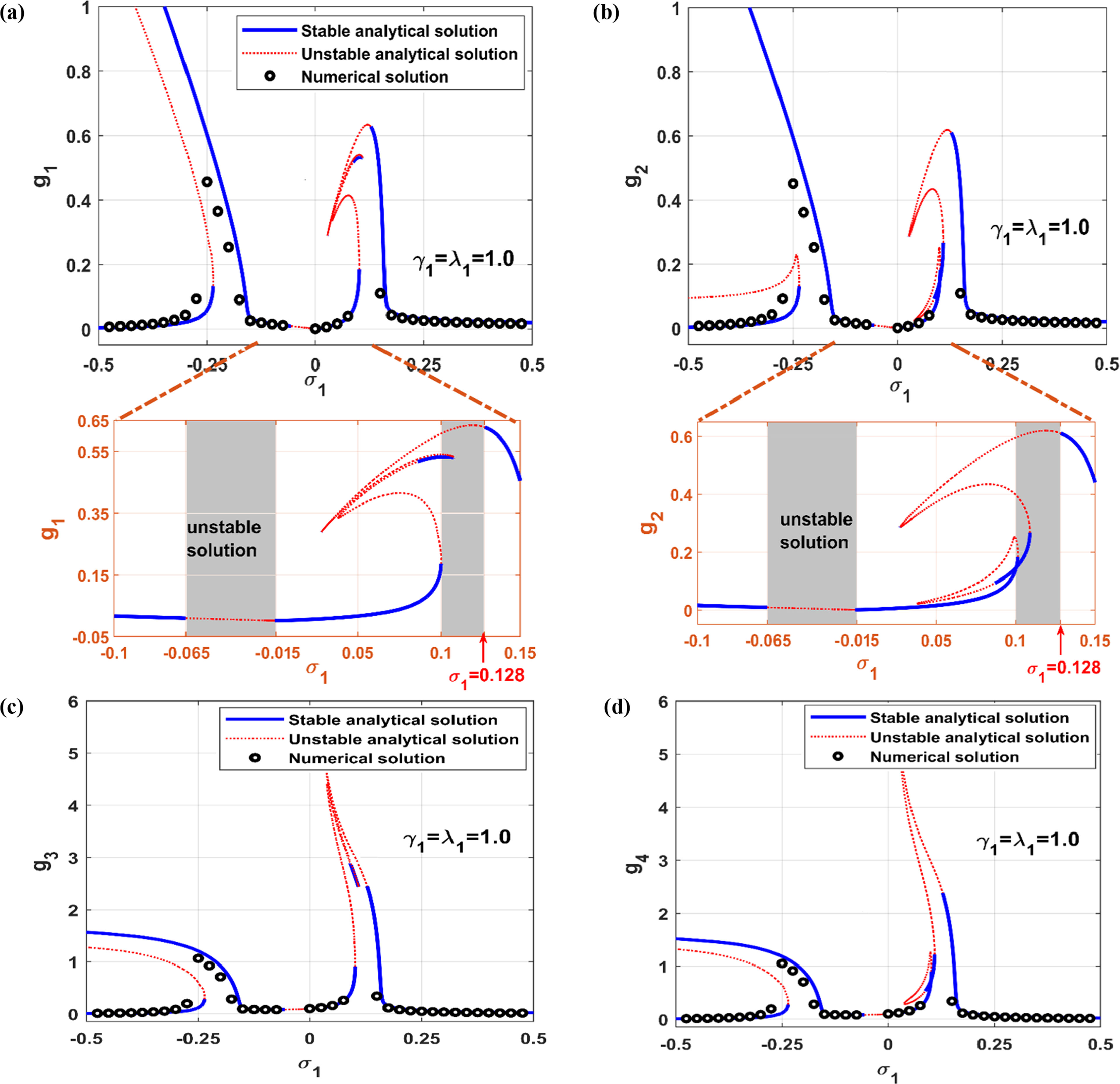
The tuned $PPFC$ was first discussed by Saeed et al. ⁴⁶ They demonstrated that tuning the $PPF{C}^{\prime }s$ natural frequency to match the excitation frequency of the vibratory system results in a complete transfer of energy from the vibratory system to the $PPFC$ , ultimately eliminating undesired vibrations in the targeted system. Accordingly, the evolution of $g_1$ and $g_2$ under the action of both controller-2 and the tuned controller-3 is illustrated in Figure 26. Tuning controller-3 involves setting ${\omega }_1$ and ${\omega }_2$ equal to the system’s angular velocity $\mathrm{\Omega }$ , which is mathematically achieved based on equation (18) when ${\sigma }_1={\sigma }_2={\sigma }_3$ . In Figure 26, the evolution of $g_1,{\hspace{0.17em}g}_2,g_3,g_4,{\hspace{0.17em}g}_5,$ and $g_6$ is plotted against ${\sigma }_1$ under the action of controller-2 and controller-3 when ${\sigma }_2={\sigma }_3=-0.25,0,$ $0.25$ , while $f_1=f_2=0.1$ and $f_3=0.03$ . It is clear from Figure 26 that $g_1=g_2\cong 0.0$ as long as ${\sigma }_1={\sigma }_2={\sigma }_3$ (i.e., $g_1=g_2\cong 0.0$ as long as ${\omega }_1={\omega }_2=\mathrm{\Omega }$ ) under controller-3. Thus, one can infer that tuning the natural frequencies ${\omega }_1$ and ${\omega }_2$ to match the rotor’s angular speed ensures the elimination of system vibrations. However, losing this tuning condition may risk the closed-loop system’s stability, potentially leading to destructive consequences.

Figure 26.

Evolution of $g_1$ and $g_2$ under controller-2 and tuned-controller-3 at different values of the detuning parameters ${\sigma }_2={\sigma }_3$ when $f_1=f_2=0.1$ and $f_3=0.03$ .

On the other hand, controller-2 cannot reduce rotor vibrations to zero due to the impossibility of achieving the tuning phenomenon. Still, it performs well along the ${\sigma }_1$ axis while ensuring closed-loop system stability. To demonstrate the accuracy of the analytical results in Figure 26, equations (11.1)–(11.6) were numerically integrated with $f_1=f_2=0.1,f_3=0.03,$ $\mathrm{\Omega }=1.0+{\sigma }_1$ , and ${\sigma }_1=0.25$ under controller-2 over the time interval $0\le \tau \le 150$ . At $\tau =150$ , controller-2 is switched off, and the tuned controller-3 (i.e., ${\sigma }_2={\sigma }_3={\sigma }_1=0.25$ ) is activated over the interval 1 $150<\tau \le 500$ , as shown in Figure 27. The figure demonstrates the elimination of system oscillations, bringing them close to zero as soon as controller-3 is activated at $\tau =150$ , which aligns with Figure 26 at ${\sigma }_1=0.25$ . In Figure 28, the evolution of $g_1,{\hspace{0.17em}g}_2,g_3,g_4,{\hspace{0.17em}g}_5,$ and $g_6$ is plotted against ${\sigma }_1$ under the influence of both controller-2 and controller-3 at three different levels of the linear parametric excitation force $f_2$ , while the other forces are held constant with $f_1=0.01$ and $f_3=0.03$ . The figure shows that the rotor’s vibration amplitudes $g_1$ and $g_2$ generally increase monotonically with $f_2$ in both cases. However, under controller-2, the two-pole rotor response remains largely stable and quasi-linear, regardless of the angular velocity or external excitation force. This behavior contrasts with controller-3, where the system may become unstable when the angular velocity deviates from the rotor’s normalized natural frequency (i.e., on both sides of ${\sigma }_1=0.0$ ). The key finding regarding controller-3 is its ability to maintain rotor oscillations near zero at perfect resonance (i.e., ${\sigma }_1=0.0$ ), regardless of the value of $f_2$ .

Figure 27.

Instantaneous temporal oscillations of the two-pole rotor model, based on the bifurcation diagram in Figure 26, with ${\sigma }_1={\sigma }_2={\sigma }_3=0.25$ : controller-2 is active and controller-3 is inactive during the time interval $0\le \tau <150$ , while controller-3 is active and controller-2 is inactive during the time interval $150\le \tau <500$ .

Figure 28.

Evolution of $g_1$ and $g_2$ under controller-2 and 3 at different levels of the linear parametric force $f_2$ , while $f_1=0.01$ and $f_3=0.03$ .

To demonstrate rotor instability under the action of controller-3 on both sides of ${\sigma }_1=0.0$ , a closer view of Figure 28 for $g_1$ and $g_2$ at $f_2=0.3$ is depicted in Figure 29. By examining Figure 29, one can observe that the two-pole rotor may lose stability under controller-3 over the intervals $-{0.027<\sigma }_1<-0.119$ and ${0.068<\sigma }_1<0.113$ , while the system remains stable under controller-2. To simulate the unstable response of the two-pole system under controller-3 versus the stable response under controller-2 along the angular speed intervals $-{0.027<\sigma }_1<-0.119$ and ${0.068<\sigma }_1<0.113$ as reported in Figure 29, equations (11.1)–(11.6) were simulated numerically corresponding to Figure 29 when ${\sigma }_1=-0.1$ (i.e., within $-{0.027<\sigma }_1<-0.119$ ) and ${\sigma }_1=0.1$ (i.e., within ${0.068<\sigma }_1<0.113$ ), as shown in Figures 30 and 31, respectively. The two figures demonstrate the small amplitude stable periodic oscillations of the rotor system under controller-2, whether ${\sigma }_1=-0.1$ or 0.1. Conversely, under controller-3, the two-pole system exhibits an unstable quasiperiodic response when ${\sigma }_1=-0.1$ and unbounded, destructive growing oscillations when ${\sigma }_1=0.1$ . By comparing the numerical simulations shown in Figures 30 and 31 with $g_1$ and $g_2$ bifurcation diagrams illustrated in Figure 29, one can confirm the excellent correspondence between the analytical and numerical solutions of equations (11.1)–(11.6).

Figure 29.

A closer view of Figures 28(a) and 28(b) when $f_2=0.3$ .

Figure 30.

Instantaneous temporal oscillations of the two-pole rotor model under controller-2 and 3, based on the bifurcation diagram in Figure 29, with ${\sigma }_1=-0.1$ : stable oscillations occur under controller-2, while quasiperiodic oscillations are observed under controller-3.

Figure 31.

Instantaneous temporal oscillations of the two-pole rotor model under controllers-2 and 3, based on the bifurcation diagram in Figure 29, with ${\sigma }_1=0.1$ : stable oscillations occur under controller-2, while growing unbounded oscillations are observed under controller-3.

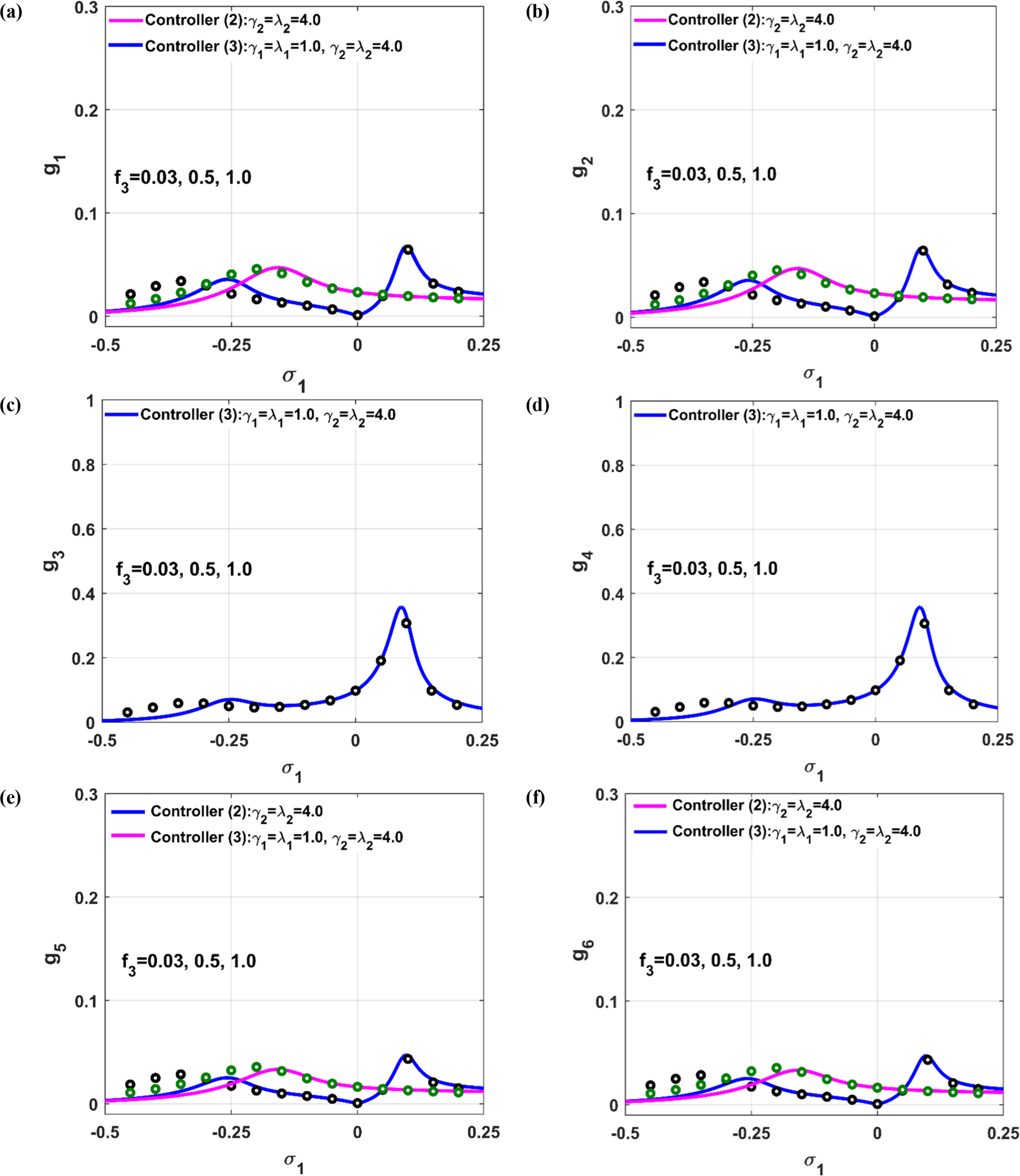
The evolution of $g_1,{\hspace{0.17em}g}_2,g_3,g_4,{\hspace{0.17em}g}_5,$ and $g_6$ is plotted against ${\sigma }_1$ under the influence of both controller-2 and controller-3 at three different levels of the nonlinear parametric excitation force $f_3$ , while the other forces are held constant at $f_1=0.01$ and $f_2=0.1$ , as shown in Figure 32. The figure demonstrates the insensitivity of the vibration amplitudes $g_1$ and $g_2$ of the system under the action of either controller-2 or controller-3. Additionally, the vibration reduction efficiency of both controllers remains competitive under the influence of the nonlinear parametric excitation force $f_3$ alone.

Figure 32.

Evolution of $g_1,{\hspace{0.17em}g}_2,g_3,g_4,{\hspace{0.17em}g}_5,$ and $g_6$ under controller-2 and controller-3 at different levels of the nonlinear parametric force $f_3$ , while $f_1=0.01$ and $f_2=0.1$ .

Dynamics of the uncontrolled versus controlled system

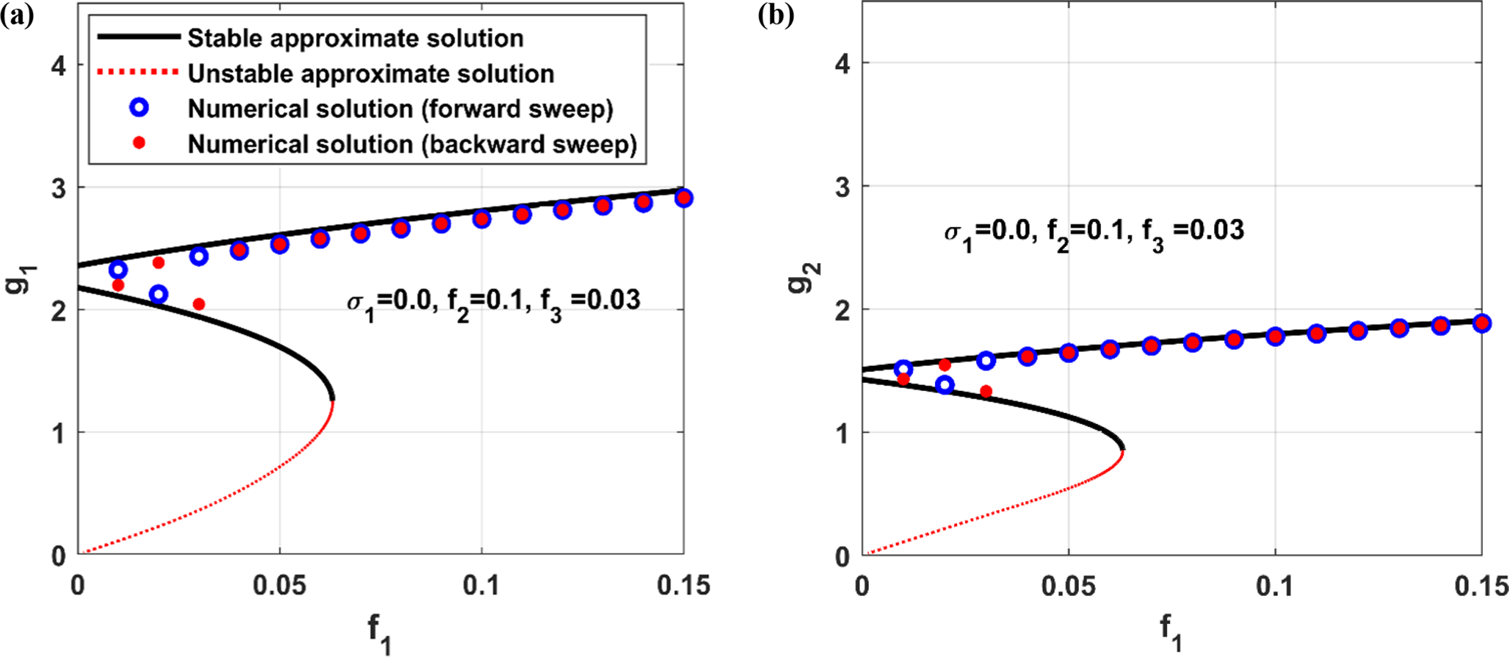
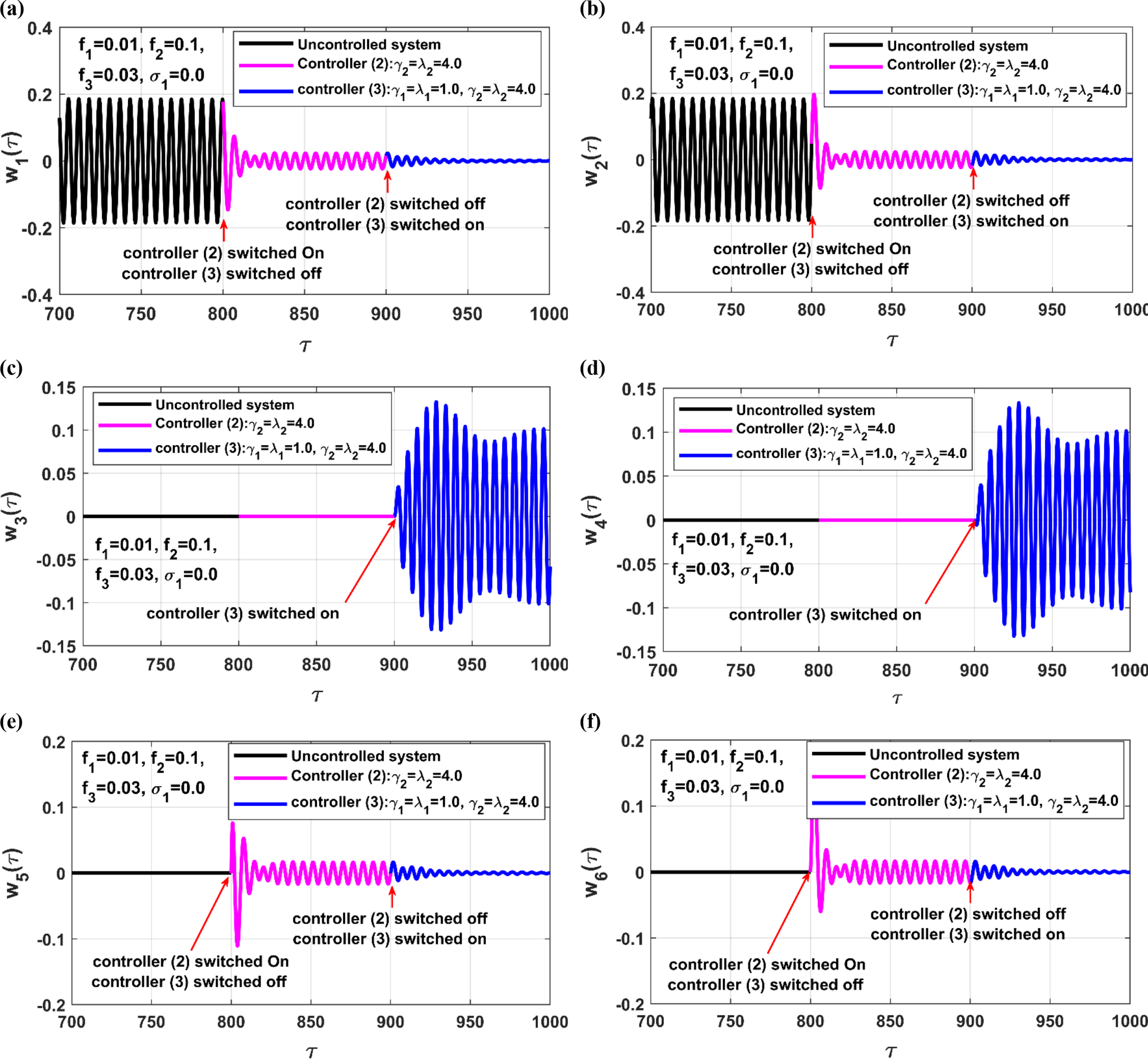
The evolution of the rotor oscillation amplitudes $g_1$ and $g_2$ against ${\sigma }_1$ is compared in Figure 33 under three conditions: before control, with Controller-2 ( ${\lambda }_2={\gamma }_2=4.0$ ), and with Controller-3 ( ${{\lambda }_1={\gamma }_1=1.0,\lambda }_2={\gamma }_2=4.0$ ) when $f_1=0.01,f_2=0.1$ and $f_3=0.03$ . It is evident from the figure that both controllers demonstrate high efficiency in suppressing resonance vibrations and mitigating the dominance of nonlinear forces. This forces the rotor to respond with a monostable solution, exhibiting a very small oscillation amplitude even under resonant conditions. Furthermore, the figure clearly illustrates the accuracy and correspondence between the analytical solutions (given by equations (23.1)–(23.8)) and the numerical simulation results, which are represented as small circles obtained by solving equations (11.1)–(11.6) using the Runge–Kutta algorithm. Additionally, the temporal oscillations of the system and controllers, both before and after control, are presented in Figure 34, corresponding to Figure 33 for ${\sigma }_1=0.0$ . This figure is generated by numerically solving equations (11.1)–(11.6) with $f_1=0.01,f_2=0.1$ and $f_3=0.03$ , and $\mathrm{\Omega }={\omega }_1={\omega }_2=1$ (i.e., ${\sigma }_1={\sigma }_2={\sigma }_3=0.0$ ) under zero initial conditions. The system is simulated without control over the time interval $0\le \tau \le 800$ . Controller-2 is activated at $\tau =800$ and remains active until $\tau =900$ . At $\tau =900$ , Controller-2 is deactivated, and Controller-3 is activated until $\tau =1000$ . The figure demonstrates strong agreement and interdependence between the analytical and numerical results.

Figure 33.

Evolution of $g_1$ and $g_2$ without control, under controller-2, and controller-3 for $f_1=0.01$ , $f_2=0.1$ , and $f=0.03$ .

Figure 34.

Instantaneous temporal oscillations of the two-pole rotor model, based on the bifurcation diagram in Figure 33, with ${\sigma }_1={\sigma }_2={\sigma }_3=0.0$ : uncontrolled system during the time interval $700\le \tau <800$ , controller-2 is active and controller-3 is inactive during the time interval $800\le \tau <900$ , while controller-3 is active and controller-2 is inactive during the time interval $900\le \tau <1000$ .

Conclusions

Vibration control of a nonlinear two-pole rotor generator system has been tackled within this article utilizing three different control strategies for the first time. The system’s equations of motion are formulated as a nonlinear two-degree-of-freedom model subjected to simultaneous external, linear parametric, and nonlinear parametric excitations. A closed-loop control system is then developed, consisting of the rotor model and the proposed control strategies, leading to six coupled nonlinear differential equations—two pairs of second-order equations and one pair of first-order equations. The three control strategies considered are $PPFC$ , $IRC$ , and a hybrid $PPFC+IRC$ approach. Using perturbation theory, an accurate analytical solution is derived for the complex closed-loop model. The following key insights and conclusions are drawn from the analysis and discussion:

(1) Despite the complexity of the closed-loop control system’s mathematical model, all analytical results align well with numerical simulations, demonstrating the accuracy of the provided solutions.

(2) Although $PPFC$ has proven effective in eliminating resonant vibrations in many harmonically excited nonlinear systems, it fails to control the asymmetric two-pole rotor due to the presence of both linear and nonlinear parametric excitations.

(3) Coupling $PPFC$ alone with the two-pole rotor via a magnetic actuator not only fails to reduce the system’s vibration but also risks destabilizing rotor motion, particularly when the angular velocity is significantly above or below the natural frequency. This can lead to quasiperiodic or unbounded oscillations, potentially causing destructive outcomes for the system.

(4) Despite its simplicity, $IRC$ successfully stabilizes the two-pole rotor vibrations under simultaneous external, linear parametric, and nonlinear parametric harmonic excitations. This forces the system to behave like a linear one, with maximum oscillations occurring at perfect resonance.

(5) While the hybrid $PPFC+IRC$ strategy offers higher performance in eliminating resonant vibrations, it can destabilize the rotor, particularly at angular velocities exceeding the first critical speed.

(6) The tuned $PPFC+IRC$ configuration is the most efficient in eliminating vibrations in the two-pole rotor model under simultaneous external, linear, and nonlinear parametric excitations. However, losing the tuning conditions not only reduces its vibration suppression efficiency but also risks destabilizing the entire closed-loop system, potentially leading to severe consequences.

(7) Ultimately, $PPFC$ is not a viable control option for this application, while $IRC$ stands out as a simpler and more stable alternative. Though the tuned $PPFC+IRC$ demonstrates superior vibration suppression, it is more complex to analyze and design compared to the reliable and straightforward $IRC$ strategy.

Future work could extend the current study by incorporating the effects of time-varying system parameters, such as temperature- and humidity-induced variations in material properties. Accounting for these factors would require modeling the system as a time-dependent dynamical system and exploring alternative control strategies, such as adaptive or AI-driven control, in comparison to the conventional methods employed in this study. This extension would enhance the robustness and practical applicability of the proposed control approach for real-world rotating machinery operating under varying environmental conditions.