On oscillation modes and basins of attraction of a harmonically excited 2-DOF cart model oscillating over an inclined surface under 1:1 internal resonance

Abstract

The nonlinear dynamics of a 2-DOF cart model system oscillating over an inclined surface are explored in this work. The considered structure consists of two subsystems: Cart-1, which acts as the primary system and is modeled as a hard-spring Duffing oscillator subjected to near-resonant harmonic excitation, and Cart-2, another Duffing oscillator with either a hard or soft spring, supported by Cart-1 and oscillating over its surface at an inclination angle $\theta$ relative to the horizontal direction. Using the Lagrange formulation, the mathematical model of the entire system is derived, and the corresponding normalized equations of motion are obtained. Utilizing multiple time-scale techniques, the autonomous slow-flow dynamical system governing the modulated amplitudes and phases of the 2-DOF cart model is extracted. By applying the continuation algorithm, the evolution of oscillation amplitudes as functions of the excitation force and frequency is analyzed, revealing various response curves. In terms of Poincaré return maps, bifurcation diagrams, basins of attraction, the $0–1$ chaos test, and stability charts, all established response curves are validated numerically. The analysis reveals that the studied system exhibits six oscillation modes, depending on both the excitation force and frequency. These modes include monostable, bistable, and tristable periodic solutions, period-n solution, a mono-quasiperiodic solution, and the coexistence of monostable periodic and mono-quasiperiodic solutions. Furthermore, it is found that Cart-2 functions as an effective vibration absorber under linear coupling with Cart-1. However, softening nonlinear stiffness coupling between the two carts induces unbounded oscillations, which could ultimately compromise the structural integrity of the coupled subsystems. This study contributes to the fields of passive vibration control and transportation system safety and stability, offering valuable insights for the design and optimization of coupled oscillatory systems with varying orientations in diverse engineering applications.

Introduction

In most mechanical systems, vibrations are inevitable and often pose significant challenges. These oscillations are commonly seen as undesirable and potentially damaging, exerting stress on components, causing wear, fatigue, and even cracks in critical parts like shafts, gears, or brake disks, ultimately leading to system failure. Such forces reduce the lifespan of machines and structures and impair system efficiency and functionality. For instance, wing oscillations in aircraft can reduce aerodynamic performance, while in rotating machinery or civil structures, vibrations threaten safety and stability, making vibration control vital in mechanical engineering.^1,2 Yet, vibrations are not solely harmful but also they can serve as diagnostic signals. Machines act as both sources and receivers of vibration, and analyzing these signals through frequency response and spectrum analysis enables early fault detection and enhances reliability. ³ Moreover, vibrations generate side effects like heat and noise, degrading performance and creating discomfort for people nearby. These effects can harm human health and the environment, especially in continuously operating systems. Noise pollution and overheating not only reduce comfort but also accelerate material degradation. The interplay of these factors highlights the importance of effectively minimizing vibrations. Proper vibration management extends equipment life and enhances efficiency, safety, and user comfort in a variety of applications.^4,5

Vibration control strategies are broadly categorized into passive, active, semi-active, and hybrid approaches. Passive control relies on materials or structures like dampers, isolators, and absorbers that dissipate vibration energy without external power. These methods, often using viscoelastic materials, are simple and cost-effective but may underperform when vibration conditions vary significantly. ⁶ Active control employs sensors, actuators, and controllers to detect and counteract vibrations in real-time, offering high adaptability and performance across diverse conditions.^7–13 However, these systems require external power and can be complex and costly to implement.^14–16 Semi-active control combines elements of both passive and active systems. Instead of injecting energy, it adjusts passive properties like stiffness or damping in response to operating conditions, offering improved adaptability with lower power demands than active systems. ¹⁷ Hybrid control blends passive, active, and/or semi-active methods to maximize the strengths of each. For example, passive components may address low-frequency disturbances while active elements target high-frequency or time-varying vibrations. Although highly effective, hybrid systems are the most complex to design and implement.^18,19 Simplicity and reliability make passive vibration absorbers popular. The Tuned Mass Damper (TMD), with a mass, spring, and damper on the main frame, is very effective. It absorbs and dissipates vibration energy to stabilize and limit motion. TMDs are selected to match vibration frequencies and work with the structure’s intrinsic modes to inhibit oscillations. The TMD can lower overall vibration levels and increase structural stability because of this interaction, which is called modal coupling. This is particularly helpful in large buildings, bridges, and mechanical systems that are prone to oscillations. Vibration absorbers were first introduced in the late 19th century to reduce ship rolling, with the earliest method proposed by Watts in 1883. In the 1930s, Den Hartog developed a systematic design approach for TMDs, paving the way for their use across various sectors. TMDs are now widely applied in civil structures and mechanical systems. For instance, Taylor ²⁰ studied their role in improving the performance of radial aircraft engines by eliminating crankshaft torsional vibrations. Keye et al. ²¹ further enhanced their application in turboprop aircraft using variable eigenfrequency designs. Setareh and Hanson ²² demonstrated their effectiveness in controlling vibrations in balconies and stands, while Newland ²³ applied them to the London Millennium Bridge to reduce wind-induced motion. Casalotti et al. ²⁴ advanced their use by integrating hysteretic dampers in suspension bridges. Habib and Kerschen ²⁵ contributed to nonlinear vibration absorber designs like the Nonlinear Energy Sink (NES) and Nonlinear Tuned Vibration Absorber (NTVA), which are better suited for systems exhibiting nonlinear behavior. Lu et al. ²⁶ reviewed nonlinear dissipative devices that broaden the operational frequency range of vibration absorbers. Detroux et al. ²⁷ analyzed the performance and robustness of NTVAs under various conditions. To overcome the limitations of passive systems, Cao et al. ²⁸ proposed Active Mass Dampers (AMDs), which can adapt to changing conditions using feedback control. Paknejad et al. ²⁹ further developed hybrid solutions, such as electromagnetic shunt dampers, combining passive and active mechanisms for enhanced efficiency and adaptability.

Resonance is a fundamental phenomenon in dynamic systems, occurring when the frequency of external excitation aligns with a system’s natural frequency, resulting in large oscillation amplitudes. In Duffing-type systems, resonance can produce both advantageous and destabilizing outcomes, making its understanding and control crucial for ensuring system stability, efficiency, and durability. Various studies have explored the dynamic behavior of Duffing pendulum systems to better comprehend the nature of resonance and its effects. ³⁰ Warminski and Kecik ³¹ investigated instabilities near the primary parametric resonance in a coupled damped pendulum system, offering important insights into its dynamic response. Warminski ³² examined a two-degree-of-freedom system exhibiting both regular and chaotic vibration modes due to self-excitation. Kecik and Warminski^33,34 expanded on these findings by studying a Duffing-based auto-parametric system under external excitation. Kecik and Mitura ³⁵ highlighted the dual role of a pendulum-tuned mass damper in vibration suppression and energy harvesting. Brzeski et al. ³⁶ further examined the stability and bifurcation characteristics of a pendulum suspended on a forced Duffing oscillator. These investigations collectively contribute to a deeper understanding of how resonance impacts nonlinear systems and inform strategies for vibration control and energy optimization.

Over the past few decades, numerous approximate analytical techniques have been developed to investigate the complex dynamics of nonlinear systems. Among these, two prominent methods have emerged: the multiple time-scale perturbation method (MTS) and the homotopy perturbation technique (HPT), both of which have proven highly effective in analyzing nonlinear oscillatory behavior. The MTS ³⁷ is a classical analytical technique that introduces multiple time scales to separate the fast and slow dynamics characteristic of weakly nonlinear systems. By systematically eliminating secular terms, MTS ensures that the resulting solutions remain accurate over long time intervals. This capability makes it particularly suitable for capturing resonance phenomena and amplitude-frequency interactions. Its structured framework is especially advantageous for analyzing complex systems with multiple degrees-of-freedom and mixed excitation modes,^38–41 providing deep insight into frequency-domain modulation and long-term dynamical behavior. In contrast, the HPT was originally introduced and subsequently enhanced by Prof. He and collaborators^42–44 through extensions such as the variational iteration method, ⁴⁵ frequency-based formulations, ⁴⁶ and the Enhanced HPT.^47–49 Unlike traditional perturbation methods, HPT does not require small parameters, allowing for the construction of approximate solutions through a straightforward iterative process. This makes it a powerful and flexible tool for addressing a wide range of nonlinear dynamical systems. While HPT excels in time-domain analysis due to its simplicity and adaptability, MTS offers superior capabilities in capturing frequency-domain characteristics, which are the primary focus of the present study.

In this work, the nonlinear dynamics of 2-DOF cart systems with special orientations are explored. The system under consideration consists of a primary cart (Cart-1) oscillating in the horizontal direction, modeled as a damped Duffing oscillator with cubic hard-spring nonlinearity and subjected to harmonic excitation. Cart-2, on the other hand, is modeled as another Duffing oscillator with cubic hard or soft-spring nonlinearity and is positioned to oscillate over Cart-1, which is inclined at an angle $\theta$ relative to the horizontal direction. The mathematical model of the coupled system is derived, and the corresponding normalized equations of motion are obtained. Analytical investigations are conducted using perturbation techniques, complemented by numerical simulations, including Poincaré return maps, bifurcation diagrams, basins of attraction, the 0–1 chaos test, and stability charts. Based on the introduced analysis, various complex oscillation modes of the coupled 2-DOF cart system are uncovered, including monostable, bistable, and tristable periodic solutions, as well as period-n, quasiperiodic, and coexisting oscillatory states. It is also demonstrated that Cart-2 can effectively act as a nonlinear vibration absorber when coupled linearly with Cart-1, significantly mitigating oscillations. Additionally, it is found that introducing a softening nonlinear coupling between the carts leads to unbounded responses, posing potential risks to structural safety. These findings may offer valuable insights for the design and stability assessment of nonlinear passive absorbers in mechanically coupled systems with inclined geometries.

Finaly, the rest of the paper is organized as follows: First, the formulation of the mathematical model and the derivation of the normalized equations of motion are presented. This is followed by an outlines the asymptotic analysis using the method of multiple time scales, leading to the establishment of the slow-flow equations. Next, the analytical and numerical results are discussed in detail. Subsequently, the enhanced homotopy perturbation technique is introduced, and its results are compared with those obtained from the multiple time-scale method. Finally, the paper concludes with a summary of the main findings.

System modeling and normalized equation of motion

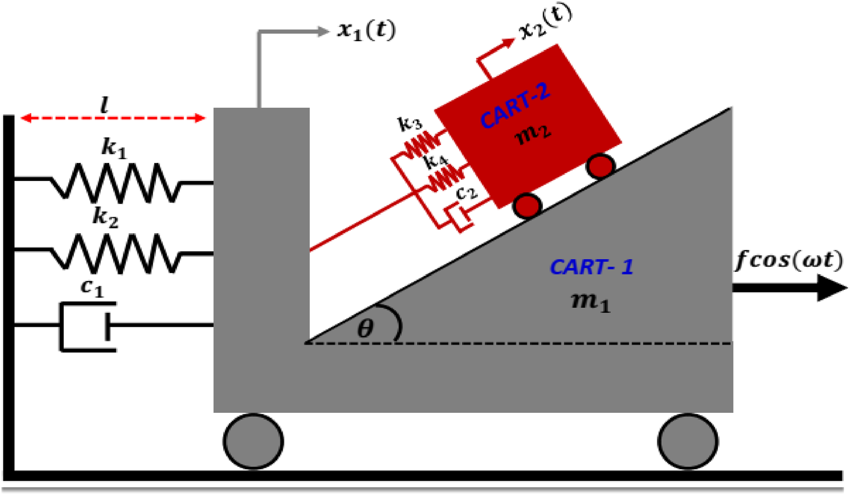
The considered 2-DOF dynamical model consists of a primary system (Cart-1) with a mass $m_1$ , coupled to a dynamic vibration absorber (Cart-2) with a mass $m_2$ , as illustrated in Figure 1. Cart-1 is connected to a fixed frame through a linear spring with a stiffness coefficient $k_1$ , a nonlinear spring with a stiffness coefficient $k_2$ , and a linear damper with a viscous damping coefficient $c_1$ . Cart-2 is connected to Cart-1 via both linear and nonlinear springs with stiffness coefficients $k_3$ and $k_4$ , respectively, as well as a linear damper with a damping coefficient $c_2$ . Cart-2 is designed to oscillate over the inclined surface of Cart-1, which forms an angle $\theta$ with the horizontal axis. The generalized coordinate system is defined by $x_1\left(t\right)$ and $x_2\left(t\right)$ , where $x_1\left(t\right)$ represents the instantaneous displacement of Cart-1 about its static equilibrium point in the horizontal direction, and $x_2\left(t\right)$ represents the instantaneous displacement of Cart-2 about its static equilibrium point along the inclined direction. Under an external harmonic excitation force $f\hspace{0.17em}\cos \left(\omega t\right)$ applied to Cart-1, the kinetic energy ( $T$ ) and potential energy ( $V$ ) of the 2-DOF system can be expressed as follows:

$T=\frac{1}{2}{m}_1{\dot{x}}_1^2+\frac{1}{2}{m}_2\left({\dot{x}}_1^2+{\dot{x}}_2^2+2\dot{x_1}\dot{x_2}\cos \left(\theta \right)\right)$

(1)

$V=\frac{1}{2}\left(k_1{x}_1^2+k_3{x}_2^2\right)+\frac{1}{4}\left(k_2{x}_1^4+k_4{x}_2^4\right)$

(2)

Figure 1.

Schematic diagram of the primary system (Cart-1) coupled with the absorber (Cart-2).

According to equations (1) and (2), the Lagrangian function ( $L$ ) can be expressed such that:

$L=T-V=\frac{1}{2}{m}_1{\dot{x}}_1^2+\frac{1}{2}{m}_2\left({\dot{x}}_1^2+{\dot{x}}_2^2+2{\dot{x}}_1{\dot{x}}_2\hspace{0.17em}\cos \left(\theta \right)\right)-\frac{1}{2}\left(k_1{x}_1^2+k_3{x}_2^2\right)-\frac{1}{4}\left(k_2{x}_1^4+k_4{x}_2^4\right)$

(3)

Following the Lagrange’s formulation, the system equations of motion can be established as follows:

$\frac{d}{dt}\left(\frac{\partial L}{\partial {\dot{x}}_1}\right)-\left(\frac{\partial L}{\partial x_1}\right)=-c_1{\dot{x}}_1+f\hspace{0.17em}\cos \left(\omega t\right)$

(4)

$\frac{d}{dt}\left(\frac{\partial L}{\partial {\dot{x}}_2}\right)-\left(\frac{\partial L}{\partial x_2}\right)=-c_2{\dot{x}}_2$

(5)

Inserting equation (3) into equations (4) and (5) yields

$\left(m_1+m_2\right){\ddot{x}}_1+m_2\hspace{0.17em}\cos \left(\theta \right){\ddot{x}}_2+k_1{x}_1+k_2{x}_1^3=-c_1{\dot{x}}_1+f\hspace{0.17em}\cos \left(\omega t\right)$

(6a)

$m_2{\ddot{x}}_2+m_2\hspace{0.17em}\cos \left(\theta \right){\ddot{x}}_1+k_3{x}_2+k_4{x}_2^3=-c_2{\dot{x}}_2$

(6b)

By introducing the dimensionless parameters $y_1=x_1/l,y_2=x_2/l,\tau ={\omega }_{n}t,M_R=m_2/m_1$ , and ${\omega }_n=\sqrt{k_1/m_1\left(1+M_R\hspace{0.17em}{\sin }^2\left(\theta \right)\right)},$ into equations (6a) and (6b) yield the following dimensionless equations of motion:

$\frac{d^2{y}_1}{d{\tau }^2}+\frac{{\mu }_1}{\sqrt{1+M_R\hspace{0.17em}{\sin }^2\left(\theta \right)}}\frac{d{y}_1}{d\tau }+{\omega }_1^2{y}_1+{\alpha }_1{y}_1^3-{\gamma }_1\frac{d{y}_2}{d\tau }-{\beta }_1{y}_2-{\beta }_2{y}_2^3=F\hspace{0.17em}\cos \left(\Omega \tau \right)$

(7a)

$\frac{d^2{y}_2}{d{\tau }^2}+\frac{\left(1+M_R\right){\mu }_2}{M_R\sqrt{1+M_R\hspace{0.17em}{\sin }^2\left(\theta \right)}}\frac{d{y}_2}{d\tau }+{\omega }_2^2{y}_2+\left(1+\frac{1}{M_R}\right){\alpha }_2{y}_2^3-{\gamma }_2\frac{d{y}_1}{d\tau }-{\beta }_3{y}_1-{\beta }_4{y}_1^3=-F\hspace{0.17em}\cos \left(\theta \right)\cos \left(\Omega \tau \right)$

(7b)

where $l$ represents the distance between Cart-1 and the vertical fixed frame at the static equilibrium position, as shown in Figure 1, ${\omega }_1=1.0,{\omega }_2=\sqrt{k_3\left(M_R+1\right)/k_1{M}_R},{\mu }_1=c_1/\sqrt{k_1{m}_1},{\mu }_2=c_2/\sqrt{k_1{m}_1},{\alpha }_1=l^2{k}_2/k_1,{\alpha }_2=l^2{k}_4/k_1,{\gamma }_1={\mu }_2\hspace{0.17em}\mathit{cos}\left(\theta \right)/\sqrt{\left(1+M_R\hspace{0.17em}{\sin }^2\left(\theta \right)\right)},{\gamma }_2={\mu }_1\hspace{0.17em}\mathit{cos}\left(\theta \right)/\sqrt{\left(1+M_R\hspace{0.17em}{\sin }^2\left(\theta \right)\right)},{\beta }_1=k_3\hspace{0.17em}\mathit{cos}\left(\theta \right)/k_1,{\beta }_2=\mathit{cos}\left(\theta \right){\alpha }_2,{\beta }_3=\mathit{cos}\left(\theta \right),{\beta }_4={\alpha }_1\hspace{0.17em}\mathit{cos}\left(\theta \right),F=f/l{k}_1,$ and $\mathrm{\Omega }=\omega /\hspace{0.17em}{\omega }_n$ . To ensure ${\omega }_2$ is always equal to ${\omega }_1=1.0$ for investigating the system’s bifurcation under 1:1 internal resonance condition, let $k_3/k_1=M_R/\left(M_R+1\right)$ . Consequently, ${\beta }_1$ can be expressed as ${\beta }_1=M_R\hspace{0.17em}\mathit{cos}\left(\theta \right)/\left(1+M_R\right)$ .

Asymptotic investigation

To analyze the bifurcation behavior of the normalized nonlinear dynamical system described by equations (7a) and (7b), an analytical solution is sought using the multiple time-scale perturbation technique, as outlined below ³⁷ :

$y_1\left(\tau ,\epsilon \right)=y_{10}\left(T_0,T_1\right)+\epsilon y_{11}\left(T_0,T_1\right)+O\left({\epsilon }^2\right)$

(8a)

$y_2\left(\tau ,\epsilon \right)=y_{20}\left(T_0,T_1\right)+\epsilon y_{21}\left(T_0,T_1\right)+O\left({\epsilon }^2\right)$

(8b)

where $T_0=\tau$ , $T_1=\epsilon \tau$ , and $\epsilon$ is a bookkeeping perturbation parameter. ³⁷ The normalized time derivatives $d/d\tau$ and $d^2/d{\tau }^2$ in equations (7a) and (7b) can be expressed in terms of $T_0$ and $T_1$ as follows:

$\frac{d}{d\tau }=D_0+\epsilon D_1,\frac{d^2}{d{\tau }^2}=D_0^2+2\epsilon D_0{D}_1,D_j=\frac{\partial }{\partial T_j},j=0,1$

(9)

To apply the solution procedure, equations (7a) and (7b) parameters are rescaled such that:

$\begin{array}{l}{\mu }_1=\epsilon {\widehat{\mu }}_1,{\mu }_2=\epsilon {\widehat{\mu }}_2,{\alpha }_1=\epsilon {\widehat{\alpha }}_1,{\alpha }_2=\epsilon {\widehat{\alpha }}_2,{\gamma }_1=\epsilon {\widehat{\gamma }}_1,{\gamma }_2=\epsilon {\widehat{\gamma }}_2,\\ {\beta }_1=\epsilon {\widehat{\beta }}_1,{\beta }_2=\epsilon {\widehat{\beta }}_2,{\beta }_3=\epsilon {\widehat{\beta }}_3,{\beta }_4=\epsilon {\widehat{\beta }}_4,F=\epsilon \widehat{F}.\end{array}\}$

(10)

By substituting equation (8a) through (10) into equations (7a) and (7b) equating the coefficients of like powers of $\epsilon$ , we obtain:

O ( ${\epsilon }^0$ )

$\left(D_0^2+{\omega }_1^2\right)y_{10}=0$

(11a)

$\left(D_0^2+{\omega }_2^2\right)y_{20}=0$

(11b)

O ( ${\epsilon }^1$ )

$\left(D_0^2+{\omega }_1^2\right)y_{11}=-2D_0{D}_1{y}_{10}-\frac{{\widehat{\mu }}_1}{\sqrt{1+M_R\hspace{0.17em}{\sin }^2\left(\theta \right)}}{D}_0{y}_{10}-{\widehat{\alpha }}_1{y}_{10}^3+{\widehat{\gamma }}_1{D}_0{y}_{20}+{\widehat{\beta }}_1{y}_{20}+{\widehat{\beta }}_2{y}_{20}^3+\widehat{F}\cos \left(\Omega T_0\right)$

(12a)

$\left(D_0^2+{\omega }_2^2\right)y_{21}=-2D_0{D}_1{y}_{20}-\frac{\left(1+M_R\right){\widehat{\mu }}_2}{M_R\sqrt{1+M_R\hspace{0.17em}{\sin }^2\left(\theta \right)}}{D}_0{y}_{20}-\left(1+\frac{1}{M_R}\right){\widehat{\alpha }}_2{y}_{20}^3+{\widehat{\gamma }}_2{D}_0{y}_{10}+{\widehat{\beta }}_3{y}_{10}+{\widehat{\beta }}_4{y}_{10}^3-\widehat{F}\cos \left(\theta \right)\cos \left(\Omega T_0\right)$

(12b)

The solution of equations (11a) and (11b), can be expressed as follows:

$y_{10}\left(T_0,T_1\right)=A\left(T_1\right)e^{i{\omega }_1{T}_0}+\overline{A}\left(T_1\right)e^{-i{\omega }_1{T}_0}$

(13a)

$y_{20}\left(T_0,T_1\right)=B\left(T_1\right)e^{i{\omega }_2{T}_0}+\overline{B}\left(T_1\right)e^{-i{\omega }_2{T}_0}$

(13b)

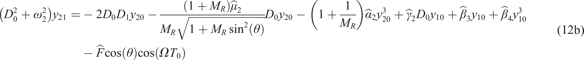
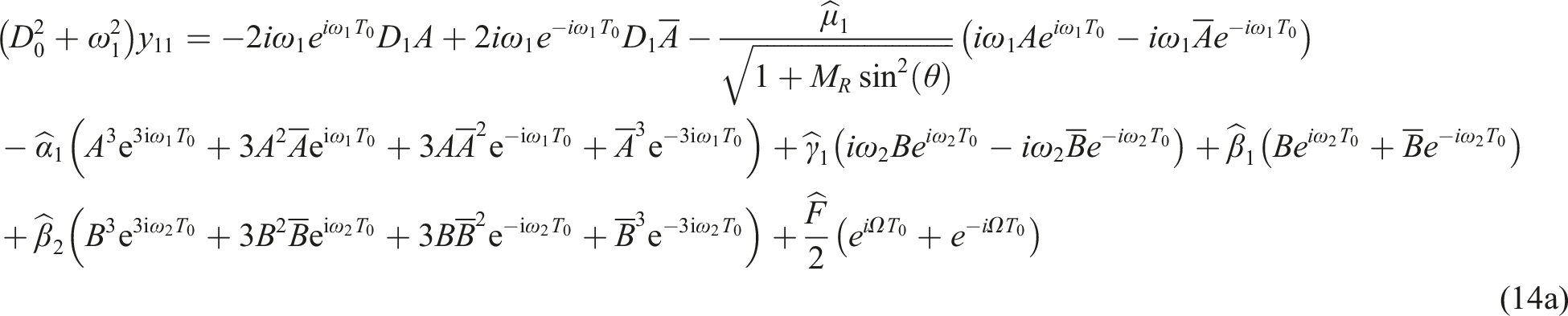
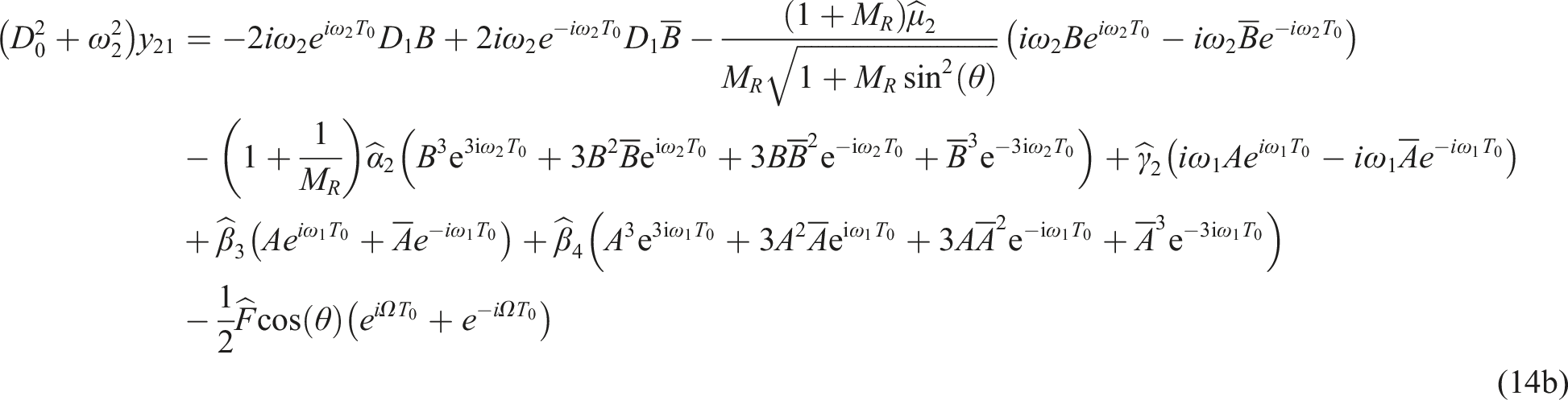
where $A\left(T_1\right)$ and $B\left(T_1\right)$ are unknown functions of ${\hspace{0.17em}T}_1$ and will be determined later. Now, by inserting equations (13a) and (13b) into equations (12a) and (12b) yield:

$\left(D_0^2+{\omega }_1^2\right)y_{11}=-2i{\omega }_1{e}^{i{\omega }_1{T}_0}{D}_{1}A+2i{\omega }_1{e}^{-i{\omega }_1{T}_0}{D}_1\overline{A}-\frac{{\widehat{\mu }}_1}{\sqrt{1+M_R\hspace{0.17em}{\sin }^2\left(\theta \right)}}\left(i{\omega }_{1}A{e}^{i{\omega }_1{T}_0}-i{\omega }_1\overline{A}{e}^{-i{\omega }_1{T}_0}\right)-{\widehat{\alpha }}_1\left(A^3{\mathrm{e}}^{3\mathrm{i}{\omega }_1{T}_0}+3A^2\overline{A}{\mathrm{e}}^{\mathrm{i}{\omega }_1{T}_0}+3A{\overline{A}}^2{\mathrm{e}}^{-\mathrm{i}{\omega }_1{T}_0}+{\overline{A}}^3{\mathrm{e}}^{-3\mathrm{i}{\omega }_1{T}_0}\right)+{\widehat{\gamma }}_1\left(i{\omega }_{2}B{e}^{i{\omega }_2{T}_0}-i{\omega }_2\overline{B}{e}^{-i{\omega }_2{T}_0}\right)+{\widehat{\beta }}_1\left(B{e}^{i{\omega }_2{T}_0}+\overline{B}{e}^{-i{\omega }_2{T}_0}\right)+{\widehat{\beta }}_2\left(B^3{\mathrm{e}}^{3\mathrm{i}{\omega }_2{T}_0}+3B^2\overline{B}{\mathrm{e}}^{\mathrm{i}{\omega }_2{T}_0}+3B{\overline{B}}^2{\mathrm{e}}^{-\mathrm{i}{\omega }_2{T}_0}+{\overline{B}}^3{\mathrm{e}}^{-3\mathrm{i}{\omega }_2{T}_0}\right)+\frac{\widehat{F}}{2}\left(e^{i\Omega T_0}+e^{-i\Omega T_0}\right)$

(14a)

$\left(D_0^2+{\omega }_2^2\right)y_{21}=-2i{\omega }_2{e}^{i{\omega }_2{T}_0}{D}_{1}B+2i{\omega }_2{e}^{-i{\omega }_2{T}_0}{D}_1\overline{B}-\frac{\left(1+M_R\right){\widehat{\mu }}_2}{M_R\sqrt{1+M_R\hspace{0.17em}{\sin }^2\left(\theta \right)}}\left(i{\omega }_{2}B{e}^{i{\omega }_2{T}_0}-i{\omega }_2\overline{B}{e}^{-i{\omega }_2{T}_0}\right)-\left(1+\frac{1}{M_R}\right){\widehat{\alpha }}_2\left(B^3{\mathrm{e}}^{3\mathrm{i}{\omega }_2{T}_0}+3B^2\overline{B}{\mathrm{e}}^{\mathrm{i}{\omega }_2{T}_0}+3B{\overline{B}}^2{\mathrm{e}}^{-\mathrm{i}{\omega }_2{T}_0}+{\overline{B}}^3{\mathrm{e}}^{-3\mathrm{i}{\omega }_2{T}_0}\right)+{\widehat{\gamma }}_2\left(i{\omega }_{1}A{e}^{i{\omega }_1{T}_0}-i{\omega }_1\overline{A}{e}^{-i{\omega }_1{T}_0}\right)+{\widehat{\beta }}_3\left(A{e}^{i{\omega }_1{T}_0}+\overline{A}{e}^{-i{\omega }_1{T}_0}\right)+{\widehat{\beta }}_4\left(A^3{\mathrm{e}}^{3\mathrm{i}{\omega }_1{T}_0}+3A^2\overline{A}{\mathrm{e}}^{\mathrm{i}{\omega }_1{T}_0}+3A{\overline{A}}^2{\mathrm{e}}^{-\mathrm{i}{\omega }_1{T}_0}+{\overline{A}}^3{\mathrm{e}}^{-3\mathrm{i}{\omega }_1{T}_0}\right)-\frac{1}{2}\widehat{F}\cos \left(\theta \right)\left(e^{i\Omega T_0}+e^{-i\Omega T_0}\right)$

(14b)

To identify the secular terms in equations (14a) and (14b), the resonance condition arises when $\mathrm{\Omega }\cong {\omega }_1$ (i.e., primary resonance) and/or ${\mathrm{\omega }}_2\cong {\omega }_1$ (1:1 internal resonance). To quantify the proximity of $\mathrm{\Omega }$ and ${\mathrm{\omega }}_2$ to ${\omega }_1$ , we introduce the new parameters ${\sigma }_1$ and ${\sigma }_2$ as follows:

$\Omega ={\omega }_1+{\sigma }_1={\omega }_1+\epsilon {\widehat{\sigma }}_1,{\sigma }_2=\epsilon {\widehat{\sigma }}_2={\omega }_2-{\omega }_1$

(15)

By inserting equation (15) into equations (14a) and (14b), we have

$\left(D_0^2+{\omega }_1^2\right)y_{11}=\left(-2i{\omega }_1{D}_{1}A-\frac{i{\omega }_1{\widehat{\mu }}_1}{\sqrt{1+M_R\hspace{0.17em}{\sin }^2\left(\theta \right)}}A-3{\widehat{\alpha }}_1{A}^2\overline{A}+i{\omega }_2{\widehat{\gamma }}_{1}B{e}^{i{\widehat{\sigma }}_2{T}_1}+{\widehat{\beta }}_{1}B{e}^{i{\widehat{\sigma }}_2{T}_1}+3{\widehat{\beta }}_2{B}^2\overline{B}{\mathrm{e}}^{i{\widehat{\sigma }}_2{T}_1}+\frac{1}{2}\widehat{F}{e}^{i{\widehat{\sigma }}_1{T}_1}\right)e^{i{\omega }_1{T}_0}+N.S.T+c.c$

(16a)

$\left(D_0^2+{\omega }_2^2\right)y_{21}=\left(-2i{\omega }_2{D}_{1}B-\frac{i{\omega }_2\left(1+M_R\right){\widehat{\mu }}_2}{M_R\sqrt{1+M_R\hspace{0.17em}{\sin }^2\left(\theta \right)}}B-3\left(1+\frac{1}{M_R}\right){\widehat{\alpha }}_2{B}^2\overline{B}+i{\omega }_1{\widehat{\gamma }}_{2}A{e}^{-i{\widehat{\sigma }}_2{T}_1}+{\widehat{\beta }}_{3}A{e}^{-i{\widehat{\sigma }}_2{T}_1}+3{\widehat{\beta }}_4{A}^2\overline{A}{e}^{-i{\widehat{\sigma }}_2{T}_1}-\frac{1}{2}\widehat{F}\cos \left(\theta \right)e^{i\left({\widehat{\sigma }}_1-{\widehat{\sigma }}_2\right)T_1}\right)e^{i{\omega }_2{T}_0}+N.S.T+c.c$

(16b)

where $N.S.T$ stands for the nonsecular term and $c.c$ denotes the complex conjugate. The solvability condition of equations (16a) and (16b) can be expressed as follows:

$-2i{\omega }_1{D}_{1}A-\frac{i{\omega }_1{\widehat{\mu }}_1}{\sqrt{1+M_R\hspace{0.17em}{\sin }^2\left(\theta \right)}}A-3{\widehat{\alpha }}_1{A}^2\overline{A}+i{\omega }_2{\widehat{\gamma }}_{1}B{e}^{i{\widehat{\sigma }}_2{T}_1}+{\widehat{\beta }}_{1}B{e}^{i{\widehat{\sigma }}_2{T}_1}+3{\widehat{\beta }}_2{B}^2\overline{B}{\mathrm{e}}^{i{\widehat{\sigma }}_2{T}_1}+\frac{1}{2}\widehat{F}{e}^{i{\widehat{\sigma }}_1{T}_1}=0$

(17a)

$-2i{\omega }_2{D}_{1}B-\frac{i{\omega }_2\left(1+M_R\right){\widehat{\mu }}_2}{M_R\sqrt{1+M_R\hspace{0.17em}{\sin }^2\left(\theta \right)}}B-3\left(1+\frac{1}{M_R}\right){\widehat{\alpha }}_2{B}^2\overline{B}+i{\omega }_1{\widehat{\gamma }}_{2}A{e}^{-i{\widehat{\sigma }}_2{T}_1}+{\widehat{\beta }}_{3}A{e}^{-i{\widehat{\sigma }}_2{T}_1}+3{\widehat{\beta }}_4{A}^2\overline{A}{e}^{-i{\widehat{\sigma }}_2{T}_1}-\frac{1}{2}\widehat{F}\cos \left(\theta \right)e^{i\left({\widehat{\sigma }}_1-{\widehat{\sigma }}_2\right)T_1}=0$

(17b)

From equation (9), we can write

$D_{1}A=\frac{d}{d{T}_1}A=\frac{d}{\epsilon d\tau }A,D_{1}B=\frac{d}{d{T}_1}B=\frac{d}{\epsilon d\tau }B$

(18)

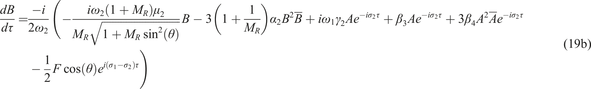
Inserting equation (18) into equations (17a) and (17b) with restoring the system parameters to nonscaled form (i.e., ${\widehat{\mu }}_1={\mu }_1/\epsilon ,{\widehat{\mu }}_2={\mu }_2/\epsilon ,{\widehat{\alpha }}_1={\alpha }_1/\epsilon ,{\widehat{\alpha }}_2={\alpha }_2/\epsilon ,{\widehat{\gamma }}_1={\gamma }_1/\epsilon ,{\widehat{\gamma }}_2={\gamma }_2/\epsilon ,{\beta }_1={\beta }_1/\epsilon ,{\widehat{\beta }}_2={\beta }_2/\epsilon ,{\beta }_3={\beta }_3/\epsilon ,{\widehat{\beta }}_4={\beta }_4/\epsilon ,{\widehat{\sigma }}_1={\sigma }_1/\epsilon ,{\widehat{\sigma }}_2={\sigma }_2/\epsilon ,\widehat{F}=F/\epsilon$ ) yields:

$\frac{dA}{d\tau }=\frac{-i}{2{\omega }_1}\left(-\frac{i{\omega }_1{\mu }_1}{\sqrt{1+M_R\hspace{0.17em}{\sin }^2\left(\theta \right)}}A-3{\alpha }_1{A}^2\overline{A}+i{\omega }_2{\gamma }_{1}B{e}^{i{\sigma }_2\tau }+{\beta }_{1}B{e}^{i{\sigma }_2\tau }+3{\beta }_2{B}^2\overline{B}{\mathrm{e}}^{i{\sigma }_2\tau }+\frac{1}{2}F{e}^{i{\sigma }_1\tau }\right)$

(19a)

$\frac{dB}{d\tau }=\frac{-i}{2{\omega }_2}\left(-\frac{i{\omega }_2\left(1+M_R\right){\mu }_2}{M_R\sqrt{1+M_R\hspace{0.17em}{\sin }^2\left(\theta \right)}}B-3\left(1+\frac{1}{M_R}\right){\alpha }_2{B}^2\overline{B}+i{\omega }_1{\gamma }_{2}A{e}^{-i{\sigma }_2\tau }+{\beta }_{3}A{e}^{-i{\sigma }_2\tau }+3{\beta }_4{A}^2\overline{A}{e}^{-i{\sigma }_2\tau }-\frac{1}{2}F\hspace{0.17em}\cos \left(\theta \right)e^{i\left({\sigma }_1-{\sigma }_2\right)\tau }\right)$

(19b)

To analyze equations (19a) and (19b), it is possible to rewrite the two functions $A$ and $B$ in their polar forms as follows ³⁷ :

$A\left(\tau \right)=\frac{1}{2}{a}_1\left(\tau \right)e^{i{\theta }_1\left(\tau \right)}\Rightarrow \hspace{1em}\frac{dA}{d\tau }=\frac{1}{2}\frac{d{a}_1}{d\tau }{e}^{i{\theta }_1}+i\frac{1}{2}{a}_1\frac{d{\theta }_1}{d\tau }{e}^{i{\theta }_1}$

(20a)

$B\left(\tau \right)=\frac{1}{2}{a}_2\left(\tau \right)e^{i{\theta }_2\left(\tau \right)}\Rightarrow \hspace{1em}\frac{dB}{d\tau }=\frac{1}{2}\frac{d{a}_2}{d\tau }{e}^{i{\theta }_2}+i\frac{1}{2}{a}_2\frac{d{\theta }_2}{d\tau }{e}^{i{\theta }_2}$

(20b)

where $a_1$ and $a_2$ are the vibration amplitudes of Cart-1 and Cart-2, respectively; ${\theta }_1$ and ${\theta }_2$ are the phases of Cart-1 and Cart-2 motions. Substituting equations (20a) and (20b) into equations (19a) and (19b) we get:

$i\frac{d{a}_1}{d\tau }+a_1\frac{d{\phi }_1}{d\tau }=a_1{\sigma }_1-\frac{1}{2}\frac{i{\mu }_1}{\sqrt{1+M_R\hspace{0.17em}{\sin }^2\left(\theta \right)}}{a}_1-\frac{3}{8{\omega }_1}{\alpha }_1{a}_1^3+\frac{1}{2{\omega }_1}i{\omega }_2{\gamma }_1{a}_2{e}^{i{\phi }_2}+\frac{1}{2{\omega }_1}{\beta }_1{a}_2{e}^{i{\phi }_2}+\frac{3}{8{\omega }_1}{\beta }_2{a}_2^3{e}^{i{\phi }_2}+\frac{1}{2{\omega }_1}F{e}^{i{\phi }_1}$

(21a)

$\begin{array}{l}i\frac{d{a}_2}{d\tau }-a_2\frac{d}{d\tau }\left({\phi }_2-{\phi }_1\right)=a_2\left({\sigma }_1-{\sigma }_2\right)-\frac{i\left(1+M_R\right){\mu }_2}{2M_R\sqrt{1+M_R\hspace{0.17em}{\sin }^2\left(\theta \right)}}{a}_2-\frac{3}{8{\omega }_2}\left(1+\frac{1}{M_R}\right){\alpha }_2{a}_2^3\\ +\frac{1}{2{\omega }_2}i{\omega }_1{\gamma }_2{a}_1{e}^{-i{\phi }_2}+\frac{1}{2{\omega }_2}{\beta }_3{a}_1{e}^{-i{\phi }_2}+\frac{3}{8{\omega }_2}{\beta }_4{a}_1^3{e}^{-i{\phi }_2}-\frac{1}{2{\omega }_2}F\hspace{0.17em}\cos \left(\theta \right)e^{i\left({\phi }_1-{\phi }_2\right)}\end{array}$

(21b)

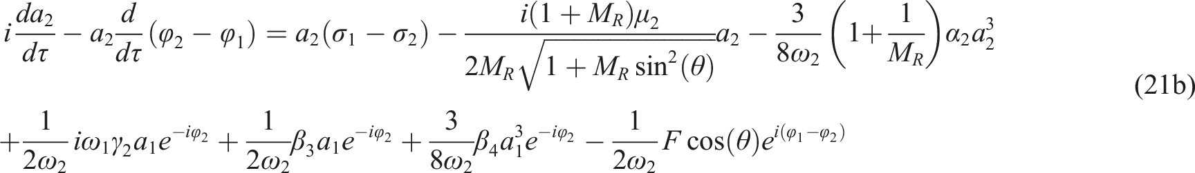
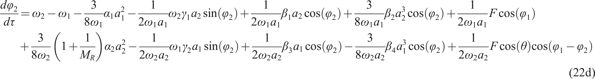
where ${\phi }_1={\sigma }_1\tau -{\theta }_1$ and ${\phi }_2={\sigma }_2\tau -{\theta }_1+{\theta }_2$ . Separating the real and imaginary parts of equations (21a) and (21b) with eliminating ${\sigma }_1$ and ${\sigma }_2$ yields:

$\frac{d{a}_1}{d\tau }=-\frac{{\mu }_1}{2\sqrt{1+M_R\hspace{0.17em}{\sin }^2\left(\theta \right)}}{a}_1+\frac{1}{2{\omega }_1}{\omega }_2{\gamma }_1{a}_2\hspace{0.17em}\cos \left({\phi }_2\right)+\frac{1}{2{\omega }_1}{\beta }_1{a}_2\hspace{0.17em}\sin \left({\phi }_2\right)+\frac{3}{8{\omega }_1}{\beta }_2{a}_2^3\hspace{0.17em}\sin \left({\phi }_2\right)+\frac{1}{2{\omega }_1}F\hspace{0.17em}\sin \left({\phi }_1\right)$

(22a)

$\frac{d{a}_2}{d\tau }=-\frac{\left(1+M_R\right){\mu }_2}{2M_R\sqrt{1+M_R\hspace{0.17em}{\sin }^2\left(\theta \right)}}{a}_2+\frac{1}{2{\omega }_2}{\omega }_1{\gamma }_2{a}_1\hspace{0.17em}\cos \left({\phi }_2\right)-\frac{1}{2{\omega }_2}{\beta }_3{a}_1\hspace{0.17em}\sin \left({\phi }_2\right)-\frac{3}{8{\omega }_2}{\beta }_4{a}_1^3\hspace{0.17em}\sin \left({\phi }_2\right)-\frac{1}{2{\omega }_2}F\hspace{0.17em}\cos \left(\theta \right)\sin \left({\phi }_1-{\phi }_2\right)$

(22b)

$\frac{d{\phi }_1}{d\tau }=\Omega -{\omega }_1-\frac{3}{8{\omega }_1}{\alpha }_1{a}_1^2-\frac{1}{2{\omega }_1{a}_1}{\omega }_2{\gamma }_1{a}_2\hspace{0.17em}\sin \left({\phi }_2\right)+\frac{1}{2{\omega }_1{a}_1}{\beta }_1{a}_2\hspace{0.17em}\cos \left({\phi }_2\right)+\frac{3}{8{\omega }_1{a}_1}{\beta }_2{a}_2^3\hspace{0.17em}\cos \left({\phi }_2\right)+\frac{1}{2{\omega }_1{a}_1}F\hspace{0.17em}\cos \left({\phi }_1\right)$

(22c)

$\frac{d{\phi }_2}{d\tau }={\omega }_2-{\omega }_1-\frac{3}{8{\omega }_1}{\alpha }_1{a}_1^2-\frac{1}{2{\omega }_1{a}_1}{\omega }_2{\gamma }_1{a}_2\hspace{0.17em}\sin \left({\phi }_2\right)+\frac{1}{2{\omega }_1{a}_1}{\beta }_1{a}_2\hspace{0.17em}\cos \left({\phi }_2\right)+\frac{3}{8{\omega }_1{a}_1}{\beta }_2{a}_2^3\hspace{0.17em}\cos \left({\phi }_2\right)+\frac{1}{2{\omega }_1{a}_1}F\hspace{0.17em}\cos \left({\phi }_1\right)+\frac{3}{8{\omega }_2}\left(1+\frac{1}{M_R}\right){\alpha }_2{a}_2^2-\frac{1}{2{\omega }_2{a}_2}{\omega }_1{\gamma }_2{a}_1\hspace{0.17em}\sin \left({\phi }_2\right)+\frac{1}{2{\omega }_2{a}_2}{\beta }_3{a}_1\hspace{0.17em}\cos \left({\phi }_2\right)-\frac{3}{8{\omega }_2{a}_2}{\beta }_4{a}_1^3\hspace{0.17em}\cos \left({\phi }_2\right)+\frac{1}{2{\omega }_2{a}_2}F\hspace{0.17em}\cos \left(\theta \right)\cos \left({\phi }_1-{\phi }_2\right)$

(22d)

Now, by substituting equations (13a), (13b), (20a), and (20b) into equations (8a) and (8b) and , we have

$y_1\left(\tau \right)=a_1\left(\tau \right)\cos \left({\omega }_1\tau +{\theta }_1\left(\tau \right)\right)=a_1\left(\tau \right)\cos \left(\Omega \tau -{\phi }_1\left(\tau \right)\right)$

(23a)

$y_2\left(\tau \right)=a_2\left(\tau \right)\cos \left({\omega }_2\tau +{\theta }_2\left(\tau \right)\right)=a_2\left(\tau \right)\cos \left(\Omega \tau -{\phi }_1\left(\tau \right)+{\phi }_2\left(\tau \right)\right)$

(23b)

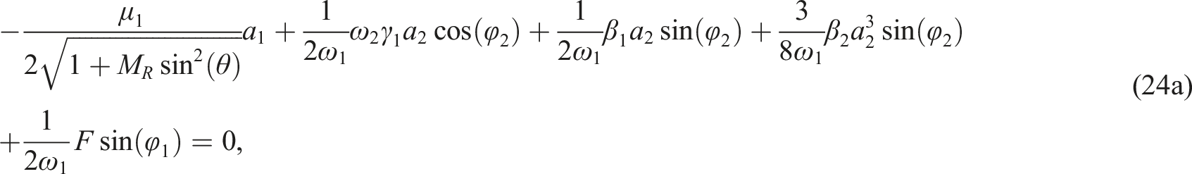
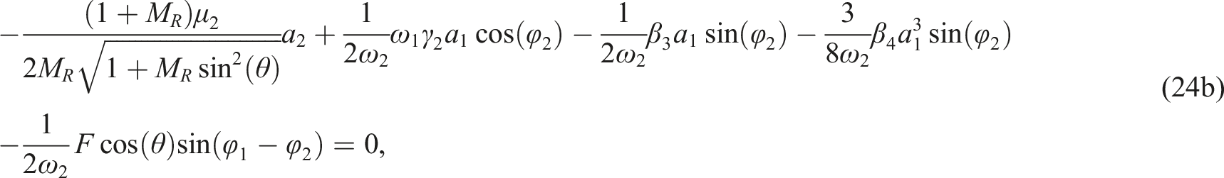
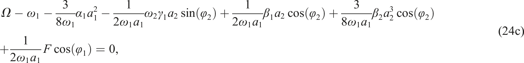
Based on equations (23a) and (23b) and , $a_1\left(\tau \right)$ and $a_2\left(\tau \right)$ represent the oscillation amplitudes of Cart-1 and Cart-2, respectively, while ${\phi }_1\left(\tau \right)$ and ${\phi }_2\left(\tau \right)$ denote the phases of the two subsystems’ motions. These time-varying functions ( $a_1\left(\tau \right),a_2\left(\tau \right),{\phi }_1\left(\tau \right)$ , and ${\phi }_2\left(\tau \right)$ ) are governed by the nonlinear autonomous dynamical system described in equations (22a)–(22d). The steady-state oscillation amplitudes and the corresponding phases of the two-cart model can be determined by analyzing the following nonlinear algebraic system, which corresponds to equations (22a)–(22d) under the condition $d{a}_1/d\tau =d{a}_2/d\tau =d{\phi }_1/d\tau =d{\phi }_2/d\tau =0$ , such that:

$\begin{array}{l}-\frac{{\mu }_1}{2\sqrt{1+M_R\hspace{0.17em}{\sin }^2\left(\theta \right)}}{a}_1+\frac{1}{2{\omega }_1}{\omega }_2{\gamma }_1{a}_2\hspace{0.17em}\cos \left({\phi }_2\right)+\frac{1}{2{\omega }_1}{\beta }_1{a}_2\hspace{0.17em}\sin \left({\phi }_2\right)+\frac{3}{8{\omega }_1}{\beta }_2{a}_2^3\hspace{0.17em}\sin \left({\phi }_2\right)\\ +\frac{1}{2{\omega }_1}F\hspace{0.17em}\sin \left({\phi }_1\right)=0,\end{array}$

(24a)

$\begin{array}{l}-\frac{\left(1+M_R\right){\mu }_2}{2M_R\sqrt{1+M_R\hspace{0.17em}{\sin }^2\left(\theta \right)}}{a}_2+\frac{1}{2{\omega }_2}{\omega }_1{\gamma }_2{a}_1\hspace{0.17em}\cos \left({\phi }_2\right)-\frac{1}{2{\omega }_2}{\beta }_3{a}_1\hspace{0.17em}\sin \left({\phi }_2\right)-\frac{3}{8{\omega }_2}{\beta }_4{a}_1^3\hspace{0.17em}\sin \left({\phi }_2\right)\\ -\frac{1}{2{\omega }_2}F\hspace{0.17em}\cos \left(\theta \right)\sin \left({\phi }_1-{\phi }_2\right)=0,\end{array}$

(24b)

$\begin{array}{l}\Omega -{\omega }_1-\frac{3}{8{\omega }_1}{\alpha }_1{a}_1^2-\frac{1}{2{\omega }_1{a}_1}{\omega }_2{\gamma }_1{a}_2\hspace{0.17em}\sin \left({\phi }_2\right)+\frac{1}{2{\omega }_1{a}_1}{\beta }_1{a}_2\hspace{0.17em}\cos \left({\phi }_2\right)+\frac{3}{8{\omega }_1{a}_1}{\beta }_2{a}_2^3\hspace{0.17em}\cos \left({\phi }_2\right)\\ +\frac{1}{2{\omega }_1{a}_1}F\hspace{0.17em}\cos \left({\phi }_1\right)=0,\end{array}$

(24c)

$\begin{array}{l}{\omega }_2-{\omega }_1-\frac{3}{8{\omega }_1}{\alpha }_1{a}_1^2-\frac{1}{2{\omega }_1{a}_1}{\omega }_2{\gamma }_1{a}_2\hspace{0.17em}\sin \left({\phi }_2\right)+\frac{1}{2{\omega }_1{a}_1}{\beta }_1{a}_2\hspace{0.17em}\cos \left({\phi }_2\right)+\frac{3}{8{\omega }_1{a}_1}{\beta }_2{a}_2^3\hspace{0.17em}\cos \left({\phi }_2\right)\\ +\frac{1}{2{\omega }_1{a}_1}F\hspace{0.17em}\cos \left({\phi }_1\right)+\frac{3}{8{\omega }_2}\left(1+\frac{1}{M_R}\right){\alpha }_2{a}_2^2-\frac{1}{2{\omega }_2{a}_2}{\omega }_1{\gamma }_2{a}_1\hspace{0.17em}\sin \left({\phi }_2\right)+\frac{1}{2{\omega }_2{a}_2}{\beta }_3{a}_1\hspace{0.17em}\cos \left({\phi }_2\right)\\ -\frac{3}{8{\omega }_2{a}_2}{\beta }_4{a}_1^3\hspace{0.17em}\cos \left({\phi }_2\right)+\frac{1}{2{\omega }_2{a}_2}F\hspace{0.17em}\cos \left(\theta \right)\cos \left({\phi }_1-{\phi }_2\right)=0.\end{array}$

(24d)

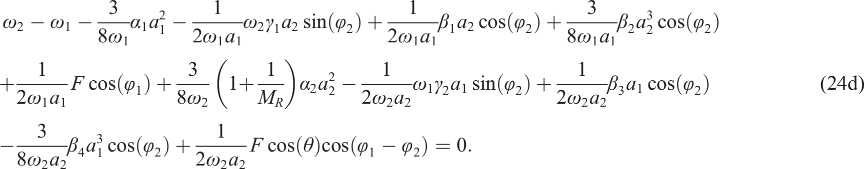
Solving equations (24a)–(24d) for $a_1,a_2,{\phi }_1,$ and ${\phi }_2$ in terms of the excitation frequency ( $\mathrm{\Omega }$ ) or excitation force amplitude ( $F$ ), while keeping other system parameters constant, yields the bifurcation diagrams. The stability of the solutions to equations (24a)–(24d) can be assessed by examining the eigenvalues of the linearized dynamical system derived from equations (23a) and (23b) and . Assuming the solution of equations (24a)–(24d) is given by $a_{10},a_{20},{\phi }_{10}$ , and ${\phi }_{20}$ , and introducing small perturbations $a_{11},a_{21},{\phi }_{11},$ and ${\phi }_{21}$ around this solution, we can mathematically express these assumptions as follows ⁵⁰ :

$\begin{array}{l}{a}_1=a_{11}+a_{10},a_2=a_{21}+a_{20},{\phi }_1={\phi }_{11}+{\phi }_{10},{\phi }_2={\phi }_{21}+{\phi }_{20}\hspace{0.17em}\Rightarrow \\ d{a}_1/d\tau =d{a}_{11}/d\tau ,d{a}_2/d\tau =d{a}_{21}/d\tau ,d{\phi }_1/d\tau =d{\phi }_{11}/d\tau ,d{\phi }_2/d\tau =d{\phi }_{21}/d\tau \end{array}\}$

(25)

Inserting equation (25) into equations (24a)–(24d), and expanding the equations for the small infinitesimals $a_{11},a_{21},{\phi }_{11},$ and ${\phi }_{21}$ , while retaining only the linear terms, yields the following linear dynamical system:

$\left(\begin{array}{l}d{a}_{11}/d\tau \\ d{\phi }_{11}/d\tau \\ d{a}_{21}/d\tau \\ d{\phi }_{21}/d\tau \end{array}\right)=\left(\begin{array}{llll}{G}_{11}& G_{12}& G_{13}& G_{14}\\ G_{21}& G_{22}& G_{23}& G_{24}\\ G_{31}& G_{32}& G_{33}& G_{34}\\ G_{41}& G_{42}& G_{43}& G_{44}\end{array}\right)\left(\begin{array}{l}{a}_{11}\\ {\phi }_{11}\\ a_{21}\\ {\phi }_{21}\end{array}\right)$

(26)

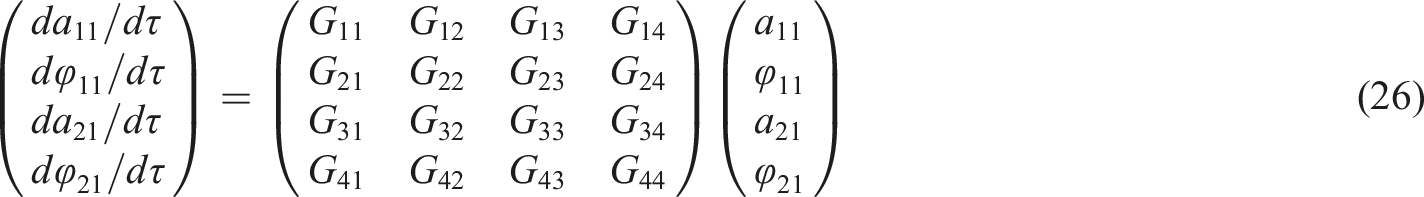
where the coefficients of the matrix in equation (26) are given in Appendix I. The eigenvalues of the above linear system can be obtained as follows:

$\left|\begin{array}{llll}{G}_{11}-\mathrm{\Delta }& G_{12}\hspace{0.17em}& G_{13}\hspace{0.17em}& G_{14}\hspace{0.17em}\\ G_{21}\hspace{0.17em}& G_{22}-\mathrm{\Delta }& G_{23}\hspace{0.17em}& G_{24}\hspace{0.17em}\\ G_{31}\hspace{0.17em}& G_{32}\hspace{0.17em}& G_{33}-\mathrm{\Delta }& G_{34}\hspace{0.17em}\\ G_{41}\hspace{0.17em}& G_{42}\hspace{0.17em}& G_{43}\hspace{0.17em}& G_{44}-\mathrm{\Delta }\end{array}\right|=0$

(27)

where $\mathrm{\Delta }$ denotes the eigenvalues. By expanding the above determinant, we have

${\mathrm{\Delta }}^4+{\rho }_1{\mathrm{\Delta }}^3+{\rho }_2{\mathrm{\Delta }}^2+{\rho }_3\mathrm{\Delta }+{\rho }_4=0$

(28)

where ${\rho }_1,{\rho }_2,{\rho }_3,$ and ${\rho }_4$ are given in Appendix II. Based on the Routh-Hurwitz criterion, the necessary and sufficient conditions for the solution of equations (24a) to (24d) to be asymptotically stable are:

${\rho }_1>0,{\rho }_1{\rho }_2-{\rho }_3>0,{\rho }_3\hspace{0.17em}\left({\rho }_1{\rho }_2-{\rho }_3\right)-{\rho }_1^2{\rho }_4>0,{\rho }_4>0$

(29)

Results and discussions

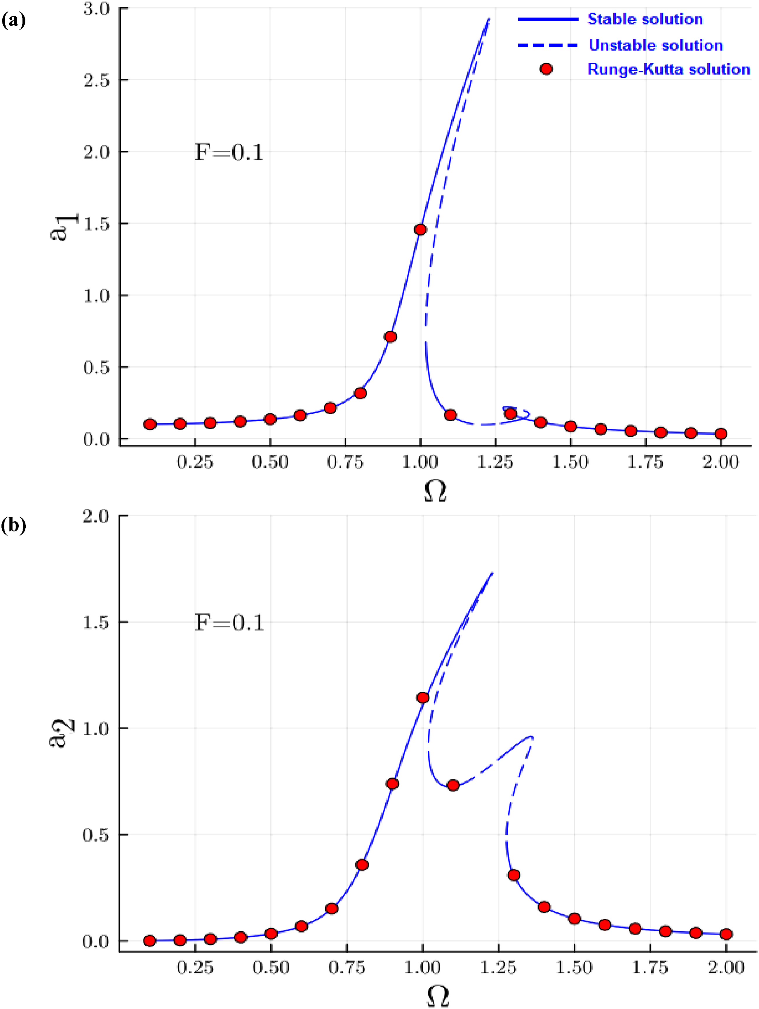
Based on the analytical investigation presented earlier, the approximate analytical solution of the normalized mathematical model for the 2-DOF cart system, governed by equations (7a) and (7b), is expressed by equations (23a) and (23b) and . The steady-state oscillation amplitudes ( $a_1$ and $a_2$ ) and phases ( ${\phi }_1$ and ${\phi }_2$ ) can be determined by solving the nonlinear algebraic system represented by equations (24a)–(24d). By numerically solving equations (24a)–(24d) for $a_1,a_2,{\phi }_1$ , and ${\phi }_2$ in terms of $\mathrm{\Omega }$ , while keeping other parameters fixed, using the Newton-Raphson continuation algorithm, ⁵¹ various bifurcation diagrams can be generated, such as those shown in Figures 2, 5, and 7. In these diagrams, stable solutions are depicted as solid lines, while unstable solutions are represented by dashed lines. Unless otherwise specified, the parameters of the normalized 2-DOF cart model are selected as follows: $F=0.1,{\omega }_1={\omega }_2=1.0,{\mu }_1=0.025,{\mu }_2=0.01,{\alpha }_1={\alpha }_2=0.1,M_R=0.1,$ and $\theta =\pi /4$ .

Figure 2.

2-DOF cart model oscillation amplitudes against $\mathrm{\Omega }$ when $F=0.1$ : solid line refers to stable periodic solution, dashed line denotes unstable periodic solution, and red circles are a numerical simulation.

Figure 2 illustrates the evolution of the oscillation amplitudes ( $a_1$ and $a_2$ ) of the 2-DOF cart model system as a function of the excitation frequency ( $\mathrm{\Omega }$ ) for $F=0.1$ . The figure highlights nonlocalized oscillations and the nonlinear interaction between the two-cart systems at $\mathrm{\Omega }={\omega }_1={\omega }_2=1.0$ , as well as the localized oscillation of Cart-2 at $\mathrm{\Omega }\cong 1.3$ . Additionally, the figure reveals the existence of various oscillation modes in the coupled system, such as monostable, bistable, and the coexistence of stable and quasiperiodic oscillations, depending on the excitation frequency. The red circles in Figure 2 represent the numerical solution of the normalized equations of motion. This solution is obtained by numerically solving equations (7a) and (7b) using the Runge-Kutta-based MATLAB algorithm ODE45. The steady-state oscillation amplitudes of $y_1\left(\tau \right)$ and $y_2\left(\tau \right)$ are plotted as red circles while incrementally increasing the excitation frequency from $\mathrm{\Omega }=0.1$ to $\mathrm{\Omega }=2.0$ with a constant step size $\mathrm{\Delta }\Omega =0.1$ . Comparing the analytical solution (solid and dashed lines) obtained by solving equations (24a)–(24d) to the numerical Runge-Kutta solution demonstrates the excellent correspondence between the two approaches, ultimately confirming the accuracy of the derived steady-state approximate solution given by equations (23a)–(24d).

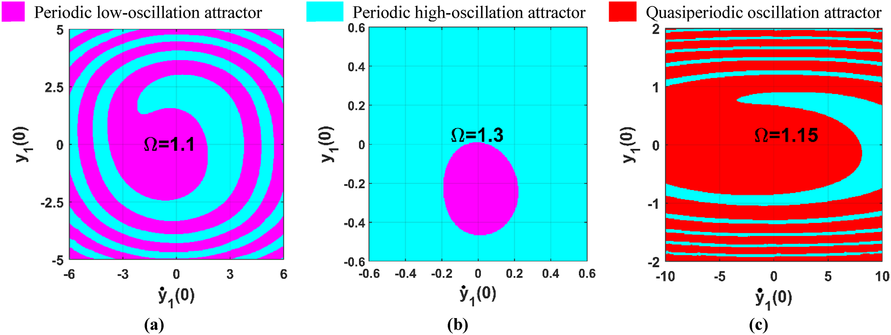
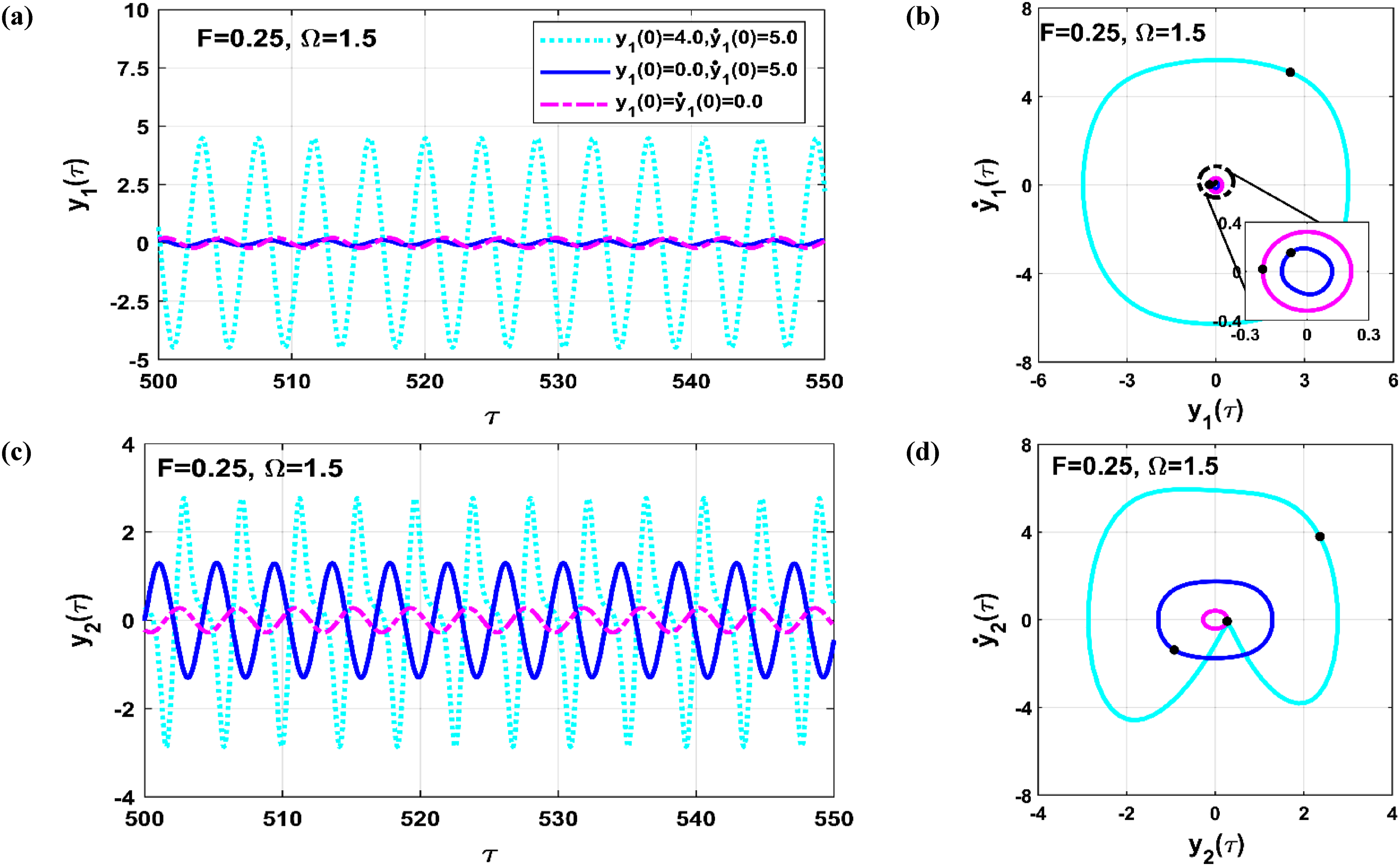
To numerically demonstrate the existence of various oscillation modes, including bistable oscillations and the coexistence of stable periodic and quasiperiodic oscillation modes in the 2-DOF cart system, the basin of attraction is established in the $y_1\left(0\right)-{\dot{y}}_1\left(0\right)$ space for three different values of $\mathrm{\Omega }$ , selected based on Figure 2. This is achieved by numerically solving equations (7a) and (7b), as illustrated in Figure 3. Figures 3(a) and 3(b) depict the system’s basin of attraction for $\mathrm{\Omega }=1.1$ and $\mathrm{\Omega }=1.3$ , respectively, while Figure 3c presents the basin of attraction for $\mathrm{\Omega }=1.15$ . In these plots, the magenta regions represent low-oscillation periodic attractors, the turquoise regions denote high-oscillation periodic attractors, and the red regions correspond to quasiperiodic attractors. From these results, it can be inferred that the 2-DOF cart model exhibits bistable oscillation modes for $\mathrm{\Omega }=1.1$ and $\mathrm{\Omega }=1.3$ . For $\mathrm{\Omega }=1.15$ , the system demonstrates the coexistence of stable periodic and quasiperiodic oscillation modes, with the specific attractor determined by the initial conditions within the magenta, turquoise, or red basins.

Figure 3.

Basins of attraction of the 2-DOF cart model in $y_1\left(0\right)-{\dot{y}}_1\left(0\right)$ space when $y_2\left(0\right)={\dot{y}}_2\left(0\right)=0.0$ , obtained corresponding to Figure 2 when: (a) $\mathrm{\Omega }=1.1$ , (b) $\mathrm{\Omega }=1.3$ , and (c) $\mathrm{\Omega }=1.15$ .

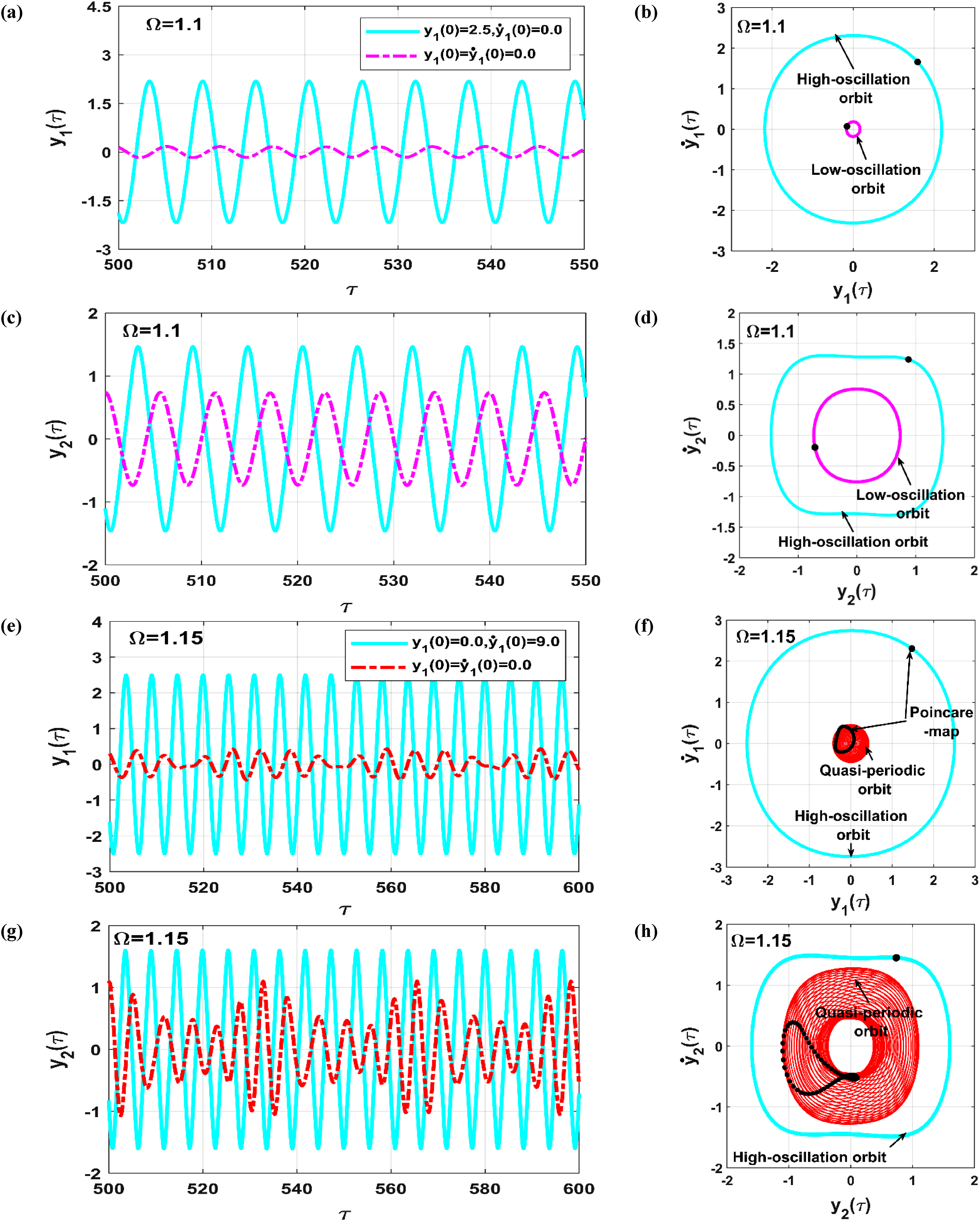
The temporal oscillations and corresponding phase-plane trajectories of the 2-DOF cart model are simulated by numerically solving equations (7a) and (7b) for various initial conditions, selected based on the basins of attraction shown in Figures 3(a) and 3(c). Figures 4(a)–4(d) illustrate the results for $\mathrm{\Omega }=1.1$ , where equations (7a) and (7b) are solved using the ODE45 algorithm. Two initial conditions are considered: $y_1\left(0\right)={\dot{y}}_1\left(0\right)=0.0$ , corresponding to the low-oscillation periodic attractor (magenta region), $y_1\left(0\right)=2.5$ and ${\dot{y}}_1\left(0\right)=0.0$ , corresponding to the high-oscillation periodic attractor (turquoise region). These results confirm that the 2-DOF cart model exhibits a bistable periodic solution at $\mathrm{\Omega }=1.1$ , where the system’s response depends on the initial position and velocity of Cart-1. Figures 4(e)–4(h) show the results for $\mathrm{\Omega }=1.15$ , again obtained using the ODE45 algorithm. Two initial conditions are analyzed: $y_1\left(0\right)={\dot{y}}_1\left(0\right)=0.0$ , corresponding to the quasiperiodic oscillation attractor (red region), and $y_1\left(0\right)=0.0$ and ${\dot{y}}_1\left(0\right)=9.0$ , corresponding to the high-oscillation periodic attractor (turquoise region). These simulations demonstrate that the 2-DOF cart model exhibits either a quasiperiodic oscillation mode or a periodic solution mode at $\mathrm{\Omega }=1.15$ , with the system’s behavior determined by the initial conditions of Cart-1.

Figure 4.

2-DOF cart model time-responses and phase-plane trajectories obtained corresponding to Figures 3(a) and 3(c): (a, b, c, d) coexistence of two stable periodic solutions (i.e., bistable oscillation mode) when $\mathrm{\Omega }=1.1$ , and (e, f, g, h) coexistence of stable periodic and quasiperiodic solution (i.e., stable periodic and quasiperiodic oscillation mode) when $\mathrm{\Omega }=1.15$ .

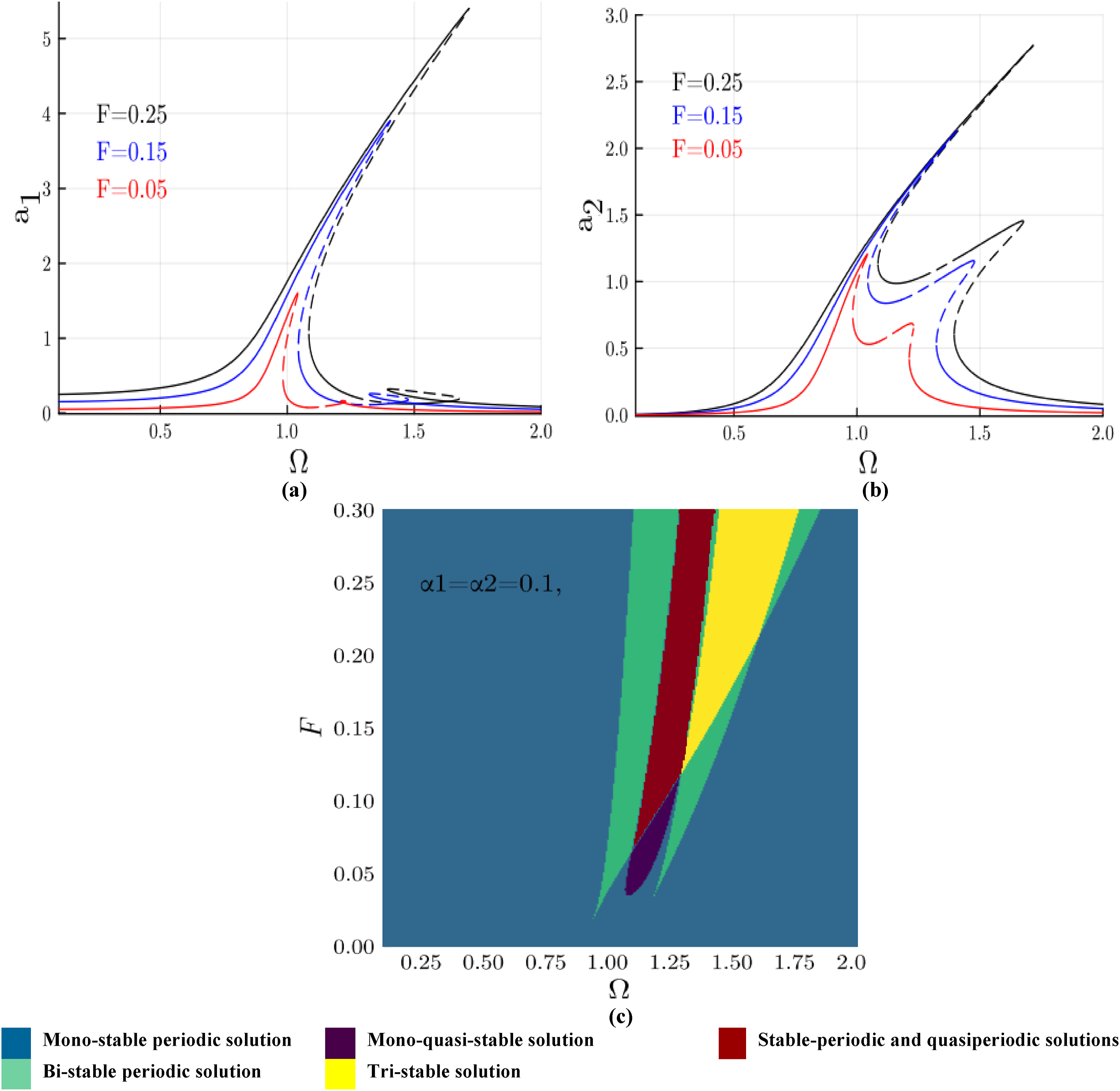
The frequency response curve of the 2-DOF cart model for varying excitation force amplitudes $F$ is visualized in Figures 5(a) and 5(b). It is evident from the figures that the oscillation amplitudes of both Cart-1 and Cart-2 monotonically increase with $F$ . Specifically, Figure 5(a) illustrates the amplitude response ( $a_1$ ) of the primary mode as a function of the excitation frequency for different forcing levels ( $F=0.05,0.15,0.25$ ). The response curves for Cart-1, depicted in Figure 5(a), exhibit characteristics typical of a single-degree-of-freedom (SDOF) system, including nonlinear features such as multi-valued solutions, resonance peaks, and the jump phenomenon. This behavior underscores the negligible influence of Cart-2 on the dynamic response of Cart-1, even under higher excitation levels ( $F=0.25$ ). In contrast, Figure 5(b) highlights the amplitude response ( $a_2$ ) of Cart-2, revealing the complex dynamics of the coupled system. This response reflects the interaction between the two modes, which gives rise to additional nonlinear phenomena such as secondary resonances and bifurcations absent in Figure 5(a). The coupling effect becomes pronounced as energy exchanges between the two modes significantly influence Cart-2’s behavior. In general, Figure 5 illustrates the transition from a simpler SDOF-like response in the first mode to a fully coupled two-degree-of-freedom (2-DOF) response. The increasing forcing amplitude amplifies the nonlinear effects in both cases. These results provide valuable insights into the intricate dynamics of coupled systems under internal resonance conditions, demonstrating multiple oscillation modes governed by both the excitation force and excitation frequency.

Figure 5.

2-DOF cart model oscillation amplitudes against $\mathrm{\Omega }$ when $F=0.05,0.15,$ and $0.25$ : (a) steady-state oscillation amplitude of Cart-1, (b) steady-state oscillation amplitude of Cart-2, and (c) stability chart in $\mathrm{\Omega }-F$ plane.

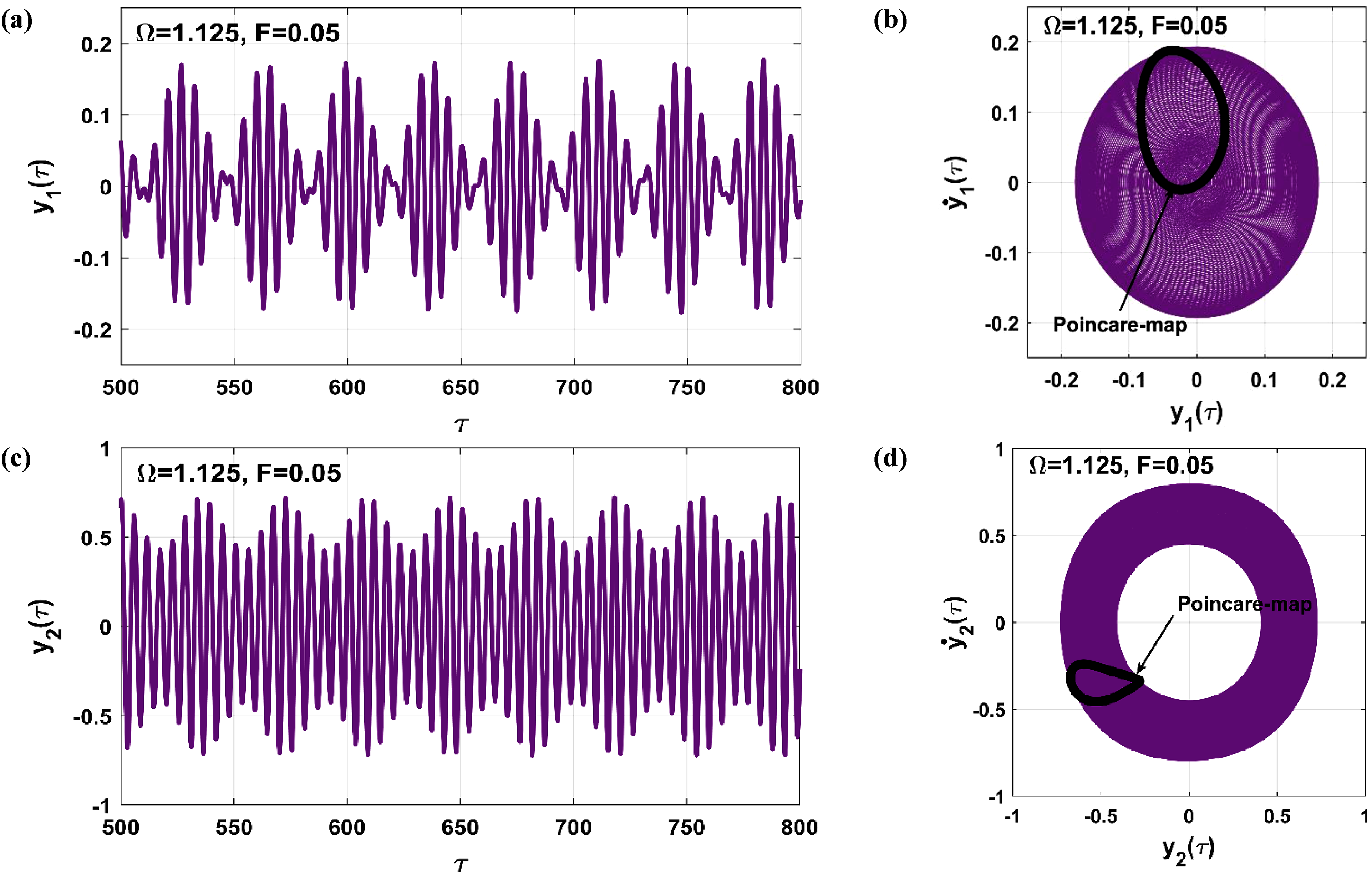
To visualize the different oscillation modes of the 2-DOF cart model in terms of $F$ and $\mathrm{\Omega }$ , the stability chart in $\mathrm{\Omega }-F$ plane is established as shown in Figure 5(c), where the figure demonstrates that the considered 2-DOF cart system can oscillate with one of five oscillation modes distinguished in different colors depending on both the excitation force and frequency. These oscillation modes are (1) monostable oscillation mode, (2) mono-quasi-stable oscillation mode, (3) bistable oscillation mode, (4) tristable oscillation mode, and (5) coexistence of stable and quasi-stable oscillation modes, all these modes are displayed with key legend as given below Figure 5(c). To visualize the various oscillation modes of the 2-DOF cart model in terms of $F$ and $\mathrm{\Omega }$ , a stability chart is established in the $\mathrm{\Omega }-F$ plane, as shown in Figure 5(c). The chart reveals that the system can oscillate in one of five distinct modes, represented by different colors based on the excitation force and frequency. These modes include the monostable oscillation mode, mono-quasi-stable oscillation mode, bistable oscillation mode, tristable oscillation mode, and the coexistence of stable and quasi-stable oscillation modes, with each mode identified using a key legend displayed below Figure 5(c). As we analytically and numerically validate the existence of the bistable oscillation mode and the coexistence of stable and quasi-stable oscillation modes, as depicted in Figure 4, the existence of a mono-quasi-stable oscillation mode is demonstrated in Figure 6. This figure is generated by numerically solving equations (7a) and (7b) with zero initial conditions for the specific point $\mathrm{\Omega }=1.125$ and $F=0.05$ , selected within the dark-purple region highlighted in Figure 6. The Poincaré maps shown in Figures 6(b) and 6(d) clearly indicate that the 2-DOF cart system exhibits a mono-quasiperiodic oscillation mode at $\mathrm{\Omega }=1.125$ and $F=0.05$ , regardless of the initial conditions.

Figure 6.

Mono-quasiperiodic oscillation mode of the 2-DOF cart model was obtained numerically corresponding to the stability chart shown in Figure 5(c) when $\mathrm{\Omega }=1.125$ and $F=0.05$ .

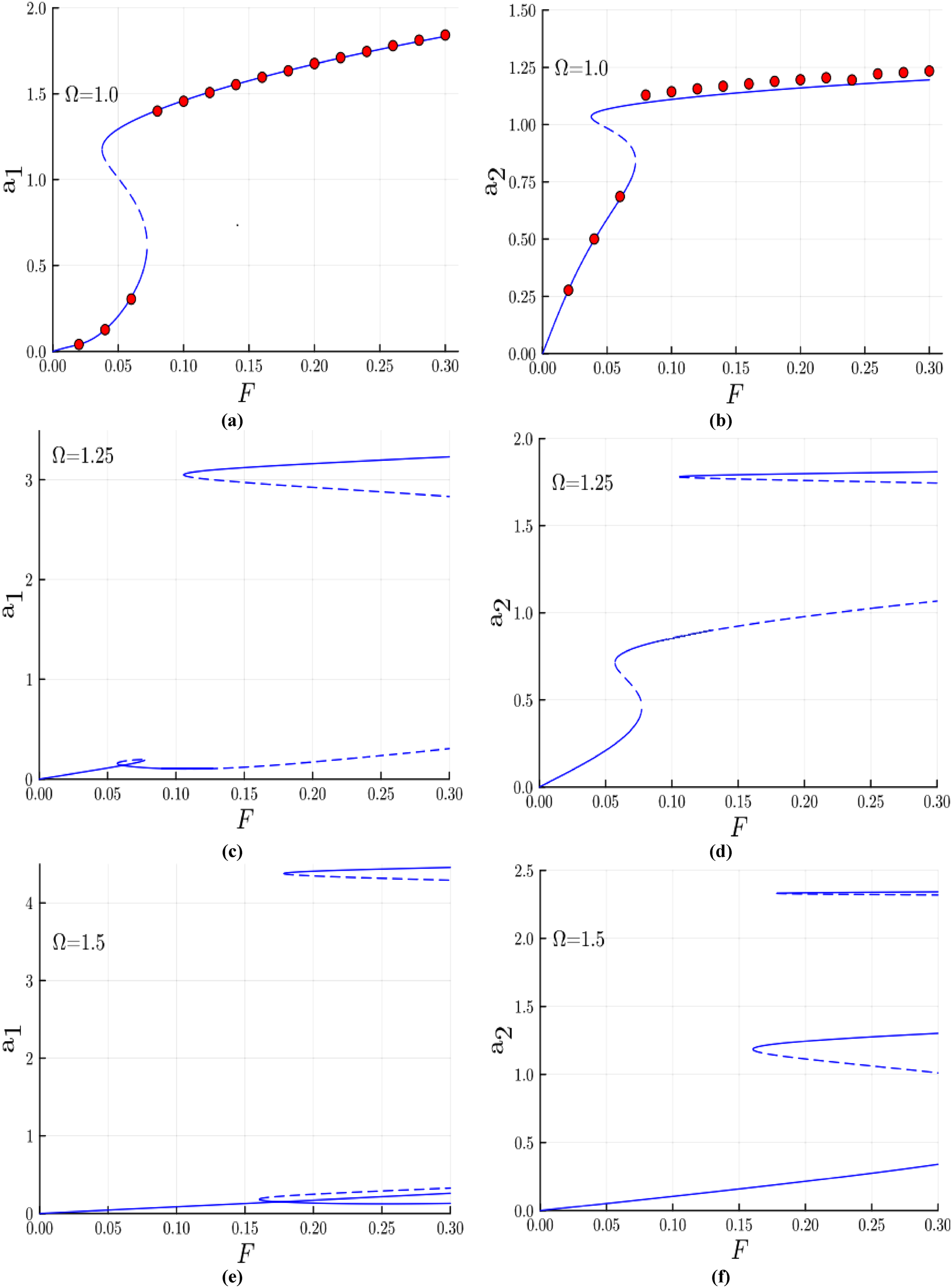
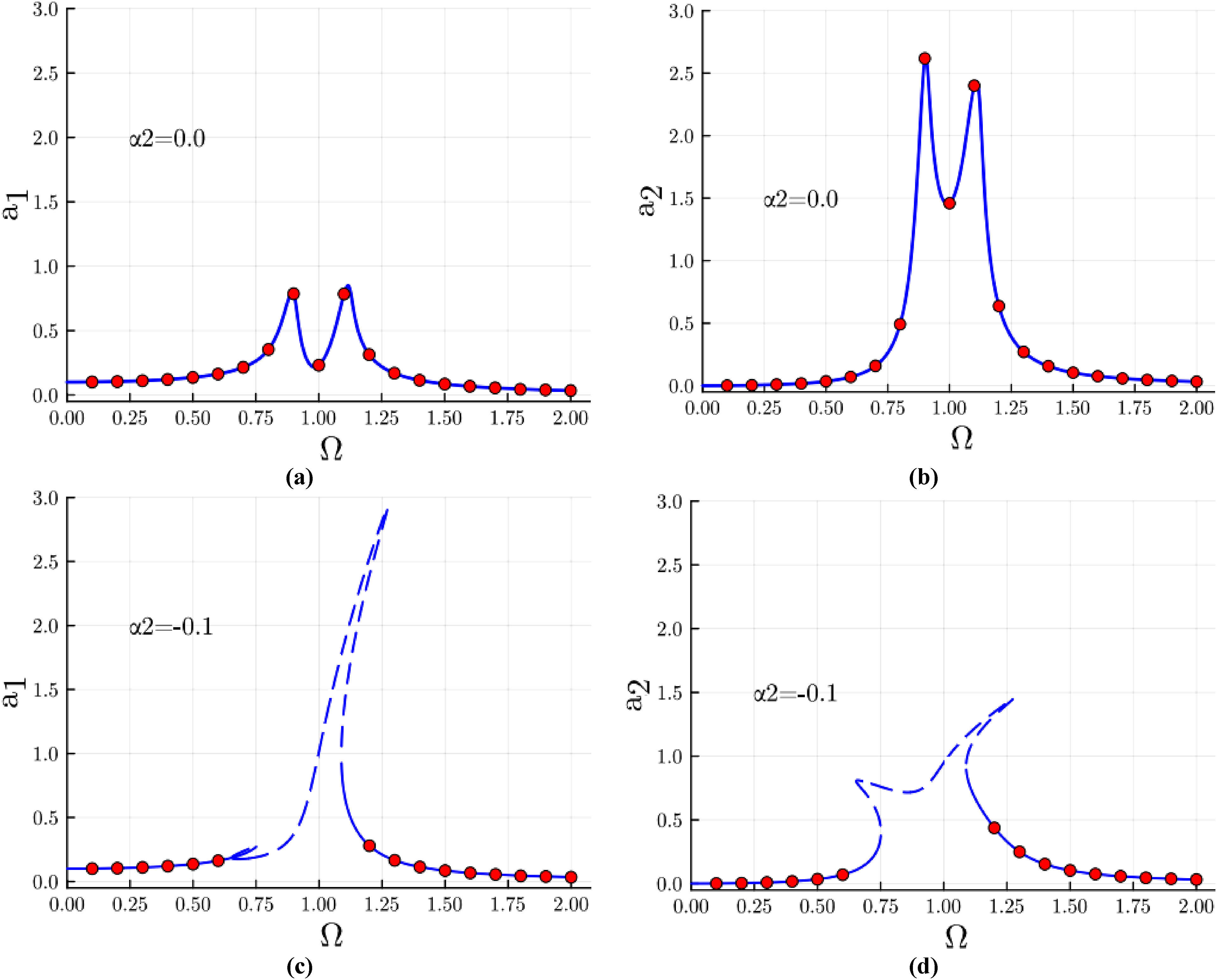
To illustrate the existence of a tristable oscillation mode, the oscillation amplitudes ( $a_1$ and $a_2$ ) of the 2-DOF cart model are plotted against $F$ for various excitation frequencies, as shown in Figure 7. Figures 7(a) and 7(b) demonstrate the existence of bistable oscillation modes within the hysteresis region and a monostable oscillation mode, represented by a curve with a unique amplitude value, under perfect resonance conditions ( $\mathrm{\Omega }={\omega }_1={\omega }_2=1.0$ ). In contrast, Figures 7(c) and 7(d) depict the evolution of $a_1$ and $a_2$ as functions of $F$ for $\mathrm{\Omega }=1.25$ . These figures reveal that the system exhibits monostable and bistable oscillation modes when $F<0.1$ . However, as $F$ increases beyond $0.1$ , the 2-DOF cart model may respond with either periodic or quasiperiodic oscillations, depending on the initial conditions of the system. Finally, Figures 7(e) and 7(f) present the evolution of $a_1$ and $a_2$ against $F$ for $\mathrm{\Omega }=1.5$ . These figures indicate that the system performs monostable periodic oscillations for $F<0.16$ , transitions to bistable oscillation modes when $0.16<F<0.18$ , and ultimately exhibits tristable oscillation modes when $F>0.18$ due to the increased excitation force amplitude.

Figure 7.

2-DOF cart model force response curves: (a, b) coexistence of monostable and bistable periodic oscillation modes depending on the magnitude of $F$ when $\mathrm{\Omega }=1.0$ , (c, d) coexistence of monostable, bistable, stable periodic, and quasiperiodic oscillation modes depending on the magnitude of $F$ when $\mathrm{\Omega }=1.25$ , and (e, f) coexistence of monostable, bistable, and tristable oscillation modes depending on the magnitude of $F$ when $\mathrm{\Omega }=1.5$ .

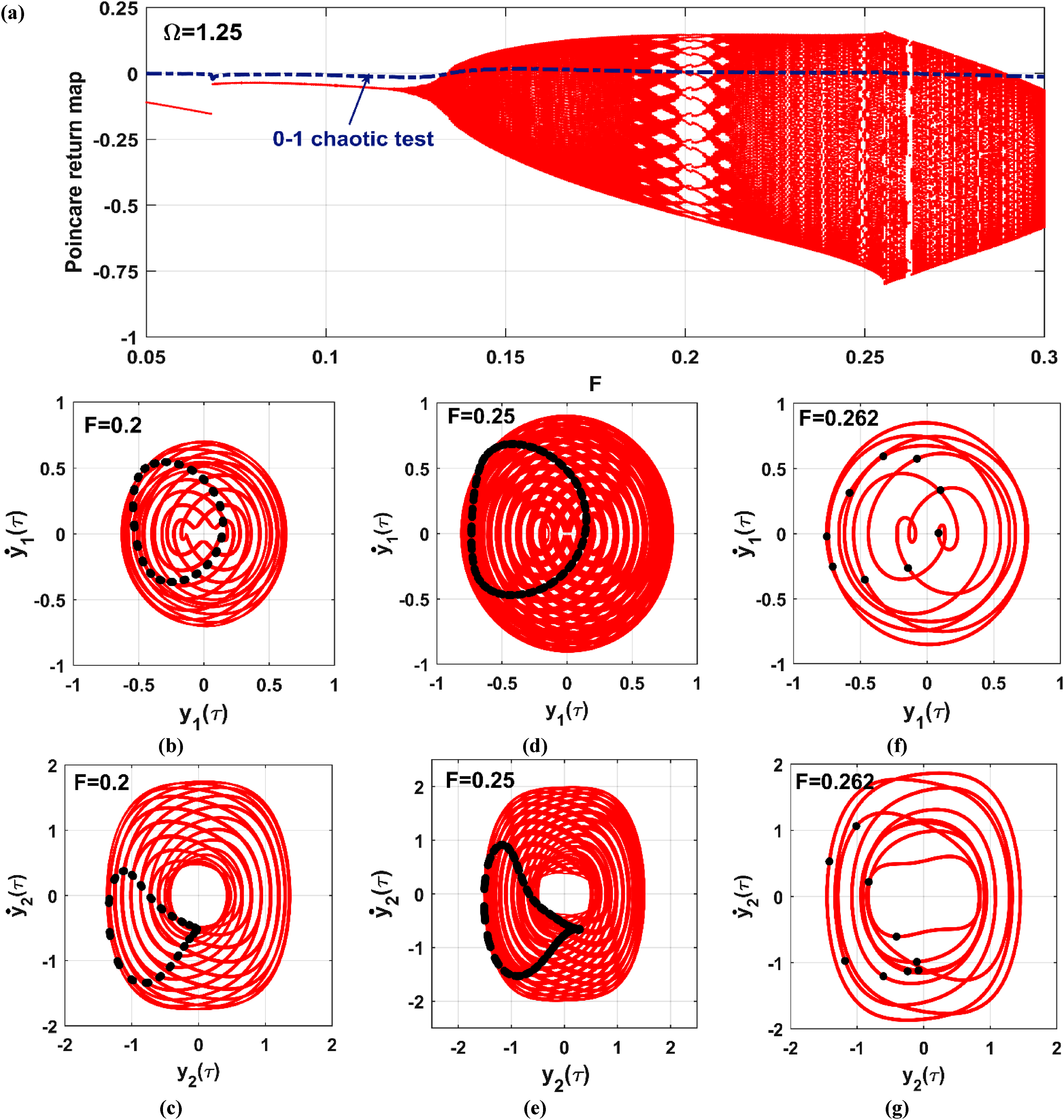
The numerical validation of the analytical results presented in Figures 7(c) and 7(d) is demonstrated in Figure 8. The bifurcation diagram of the 2-DOF cart system is constructed using $F$ as the main bifurcation parameter over the range $0.05<F\le 0.3$ for $\mathrm{\Omega }=1.25$ . This diagram, shown in Figure 8(a), is obtained by plotting the steady-state Poincaré return map for equations (7a) and (7b) against $F$ , with an incremental step size of $\mathrm{\Delta }F=0.0005$ and zero initial conditions. To further distinguish between chaotic and non-chaotic responses, the 0–1 chaos test algorithm is applied.^52,53 The algorithm’s output, represented as a dashed-dotted line in Figure 8(a), remains close to zero, indicating a non-chaotic system response. The bifurcation diagram reveals that the system exhibits periodic oscillations when $F<0.12$ . As $F$ increases beyond $0.12$ , the system transitions to period-n or quasiperiodic motions, aligning well with the results shown in Figures 7(c) and 7(d). Figure 8(b) through 8(g) illustrate the system’s phase-plane trajectories and corresponding Poincaré return maps for three specific excitation amplitude levels ( $F=0.2,0.25,0.262$ ), simulated using $\mathrm{\Omega }=1.25$ and zero initial conditions. These simulations confirm the presence of period-n motions and quasiperiodic oscillations, offering further validation of the system’s dynamic behavior.

Figure 8.

(a) 2-DOF cart model bifurcation diagram obtained numerically corresponding to Figures 7(c) and 7(d) when $\mathrm{\Omega }=1.25$ utilizing $F$ as bifurcation control parameter with zero initial conditions, (b-g) phase-plane trajectories and the corresponding Poincare map of the 2-DOF cart model obtained according to the obtained bifurcation diagram in (a) at zero initial conditions: (b, c) period-n motion when $F=0.2$ , (d, e) quasiperiodic motion when $F=0.25$ , and (f, g) period-n motion when $F=0.262$ .

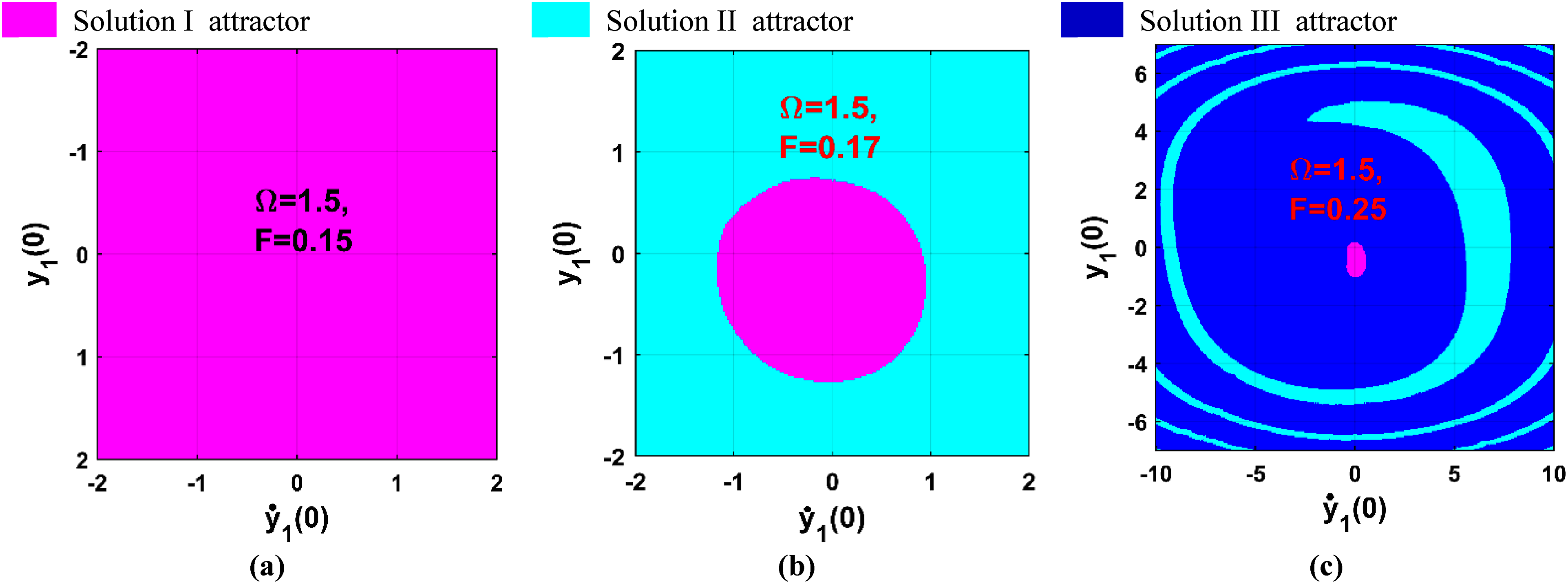
To numerically validate the presence of monostable, bistable, and tristable periodic oscillations in the system, as predicted analytically and illustrated in Figures 7(e) and 7(f) for $\mathrm{\Omega }=1.5$ under varying excitation force amplitudes ( $F$ ), the corresponding basins of attraction are presented in Figure 9. These basins are obtained by solving equations (7a) and (7b) numerically within the $y_1\left(0\right)-{\dot{y}}_1\left(0\right)$ phase space, while fixing $y_2\left(0\right)={\dot{y}}_2\left(0\right)=0.0$ , for $F=0.15,0.17,$ and $0.25$ . Figure 9 confirms the existence of monostable, bistable, and tristable periodic attractors, depending on the excitation amplitude. Specifically, monostable, bistable, and tristable behaviors are observed for $F=0.15,0.17,$ and $0.25$ , respectively. These results are in excellent agreement with the analytical predictions depicted in Figures 7(e) and 7(f), further substantiating the system’s complex dynamic response to varying excitation forces. To visualize the simultaneous existence of three stable periodic solutions in the 2-DOF cart system, corresponding to the basin of attraction established in Figure 9(c), the steady-state temporal oscillations and the associated phase-plane trajectories are illustrated in Figure 10. These are obtained by solving equations (7a) and (7b) for three distinct initial conditions selected to represent the three attractors (depicted in magenta, turquoise, and blue) shown in Figure 9(c) for $F=0.25$ and $\mathrm{\Omega }=1.5$ . Figure 10 demonstrates that the system oscillates with one of the three stable periodic solutions depending on the initial condition, confirming the tristable behavior of the 2-DOF cart system.

Figure 9.

2-DOF cart model Basins of attractions obtained according to Figures 7(e) and 7(f) when $\mathrm{\Omega }=1.5$ : (a) monostable periodic solution when $F=0.15$ , (b) bistable periodic solution when $F=0.17$ , and (c) tristable periodic solution when $F=0.25$ .

Figure 10.

Coexistence of tristable periodic motion of the 2-DOF cart model when $F=0.25$ and $\mathrm{\Omega }=1.5$ with three different initial conditions selected according to the basins of attraction shown in Figure 9(c).

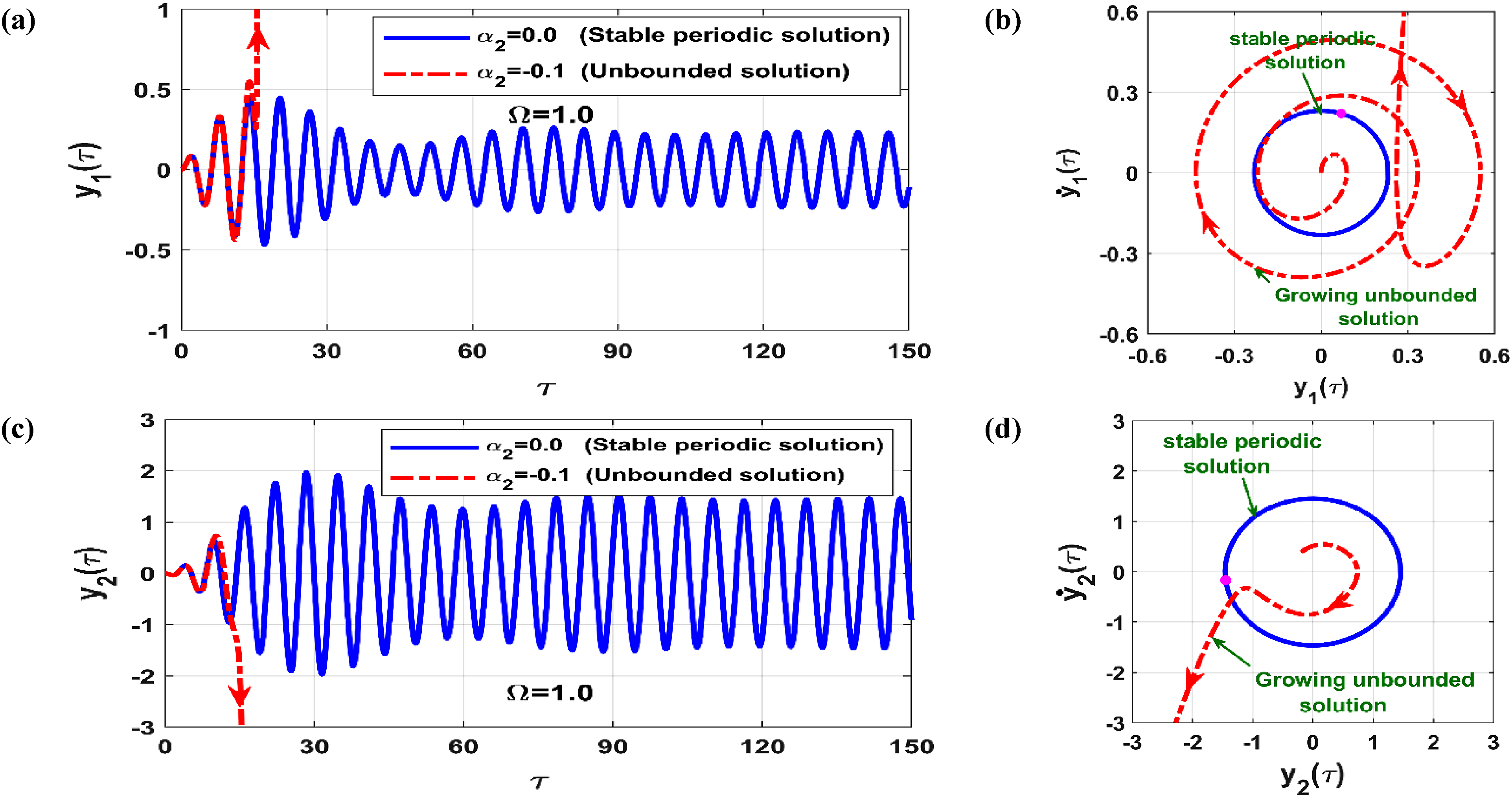
The dynamic behavior of the 2-DOF cart model for different normalized nonlinear stiffness coefficients ( ${\alpha }_2$ ) is presented in Figure 11. Figures 11(a) and 11(b) depict the evolution of $a_1$ and $a_2$ versus $\mathrm{\Omega }$ for ${\alpha }_2=0.0$ , while Figures 11(c) and 11(d) illustrate the same variables for ${\alpha }_2=-0.1$ . From Figures 11(a) and 11(b), it is evident that Cart-2 functions as a linear vibration absorber when the nonlinear stiffness coefficient is zero ( ${\alpha }_2=0.0$ ). In this case, the resonant peak of Cart-1 is effectively suppressed by establishing an energy bridge that channels vibratory motion from Cart-1 to Cart-2, even when Cart-2 is inclined at $\theta =\pi /4$ on the surface of Cart-1. Conversely, Figures 11(c) and 11(d) demonstrate that the 2-DOF cart system loses stability near the resonance condition when Cart-2 exhibits soft-spring-type nonlinear stiffness ( ${\alpha }_2<0$ ). Figure 12 further complements these findings by presenting the numerical solutions of equations (7a) and (7b) for $\mathrm{\Omega }=1.0$ with zero initial conditions, corresponding to the scenarios in Figure 11. The normalized temporal oscillations of Cart-1 and Cart-2, as well as their phase-plane trajectories, are visualized for ${\alpha }_2=0.0$ and ${\alpha }_2=-0.1$ . The results in Figure 12 confirm the stable periodic response of the 2-DOF cart system for ${\alpha }_2=0.0$ , characterized by a small oscillation amplitude of Cart-1 and a strong oscillation amplitude of Cart-2, consistent with Figures 11(a) and 11(b). In contrast, Figure 12 also reveals the unbounded response of Cart-1 and Cart-2 for ${\alpha }_2=-0.1$ , aligning with Figures 11(c) and 11(d) for $\mathrm{\Omega }=1.0$ .

Figure 11.

2-DOF cart model oscillation amplitudes against $\mathrm{\Omega }$ when ${\alpha }_2=0.0$ and $-0.1$ : (a, b) steady-state oscillation amplitudes when ${\alpha }_2=0.0$ , and (c, d) steady-state oscillation amplitudes when ${\alpha }_2=-0.1$ .

Figure 12.

Stable periodic and unbounded oscillation of the considered 2-DOF cart model corresponding to Figure 11 for $\mathrm{\Omega }=1.0$ when ${\alpha }_2=0.0$ and $-0.1$ .

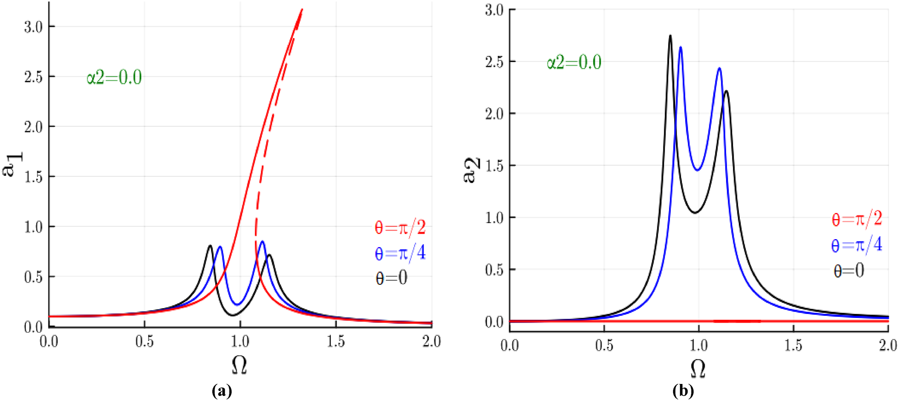
The influence of inclination angles ( $\theta$ ) on the response amplitudes of the 2-DOF cart model is analyzed in Figure 13. The figure illustrates the complete decoupling of the two oscillation modes when $\theta ={\pi /2}^o$ , where Cart-1 behaves as a single-degree-of-freedom (SDF) system under harmonic excitation, and Cart-2 remains stationary in its equilibrium position. Conversely, full interaction between Cart-1 and Cart-2 is observed when $\theta =0^o$ (i.e., Cart-2 oscillates horizontally along the surface of Cart-1). In this configuration, Cart-2 effectively functions as a linear vibration absorber. Thus, the inclination angle serves as a control mechanism for fully or partially coupling the oscillation modes of the 2-DOF cart system. This dynamic interplay offers the potential for tuning the system’s response based on the desired level of coupling or decoupling between the carts depending on the application required.

Figure 13.

Effect of the inclination angle $\theta$ on the response amplitudes of the considered 2-DOF cart model when ${\alpha }_2=0.0$ .

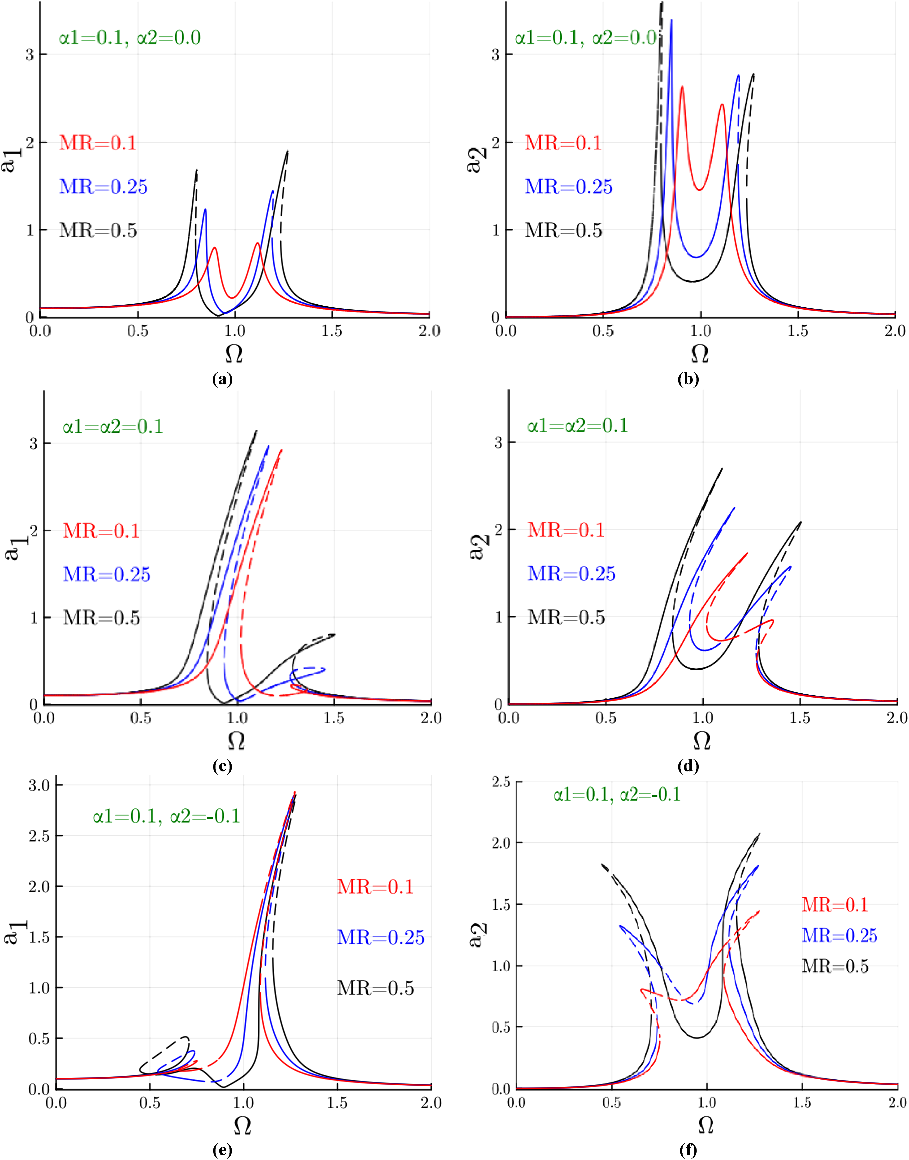
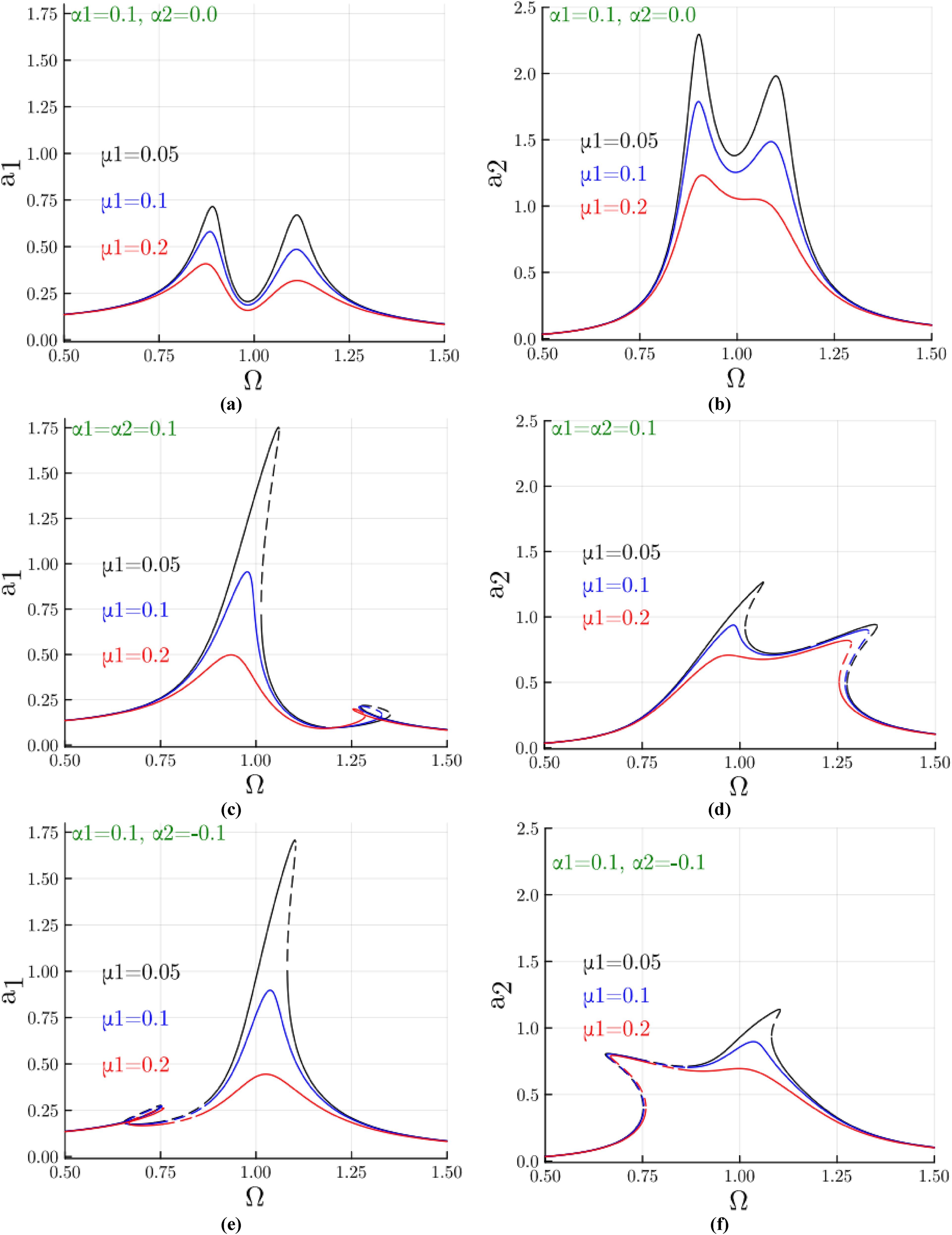
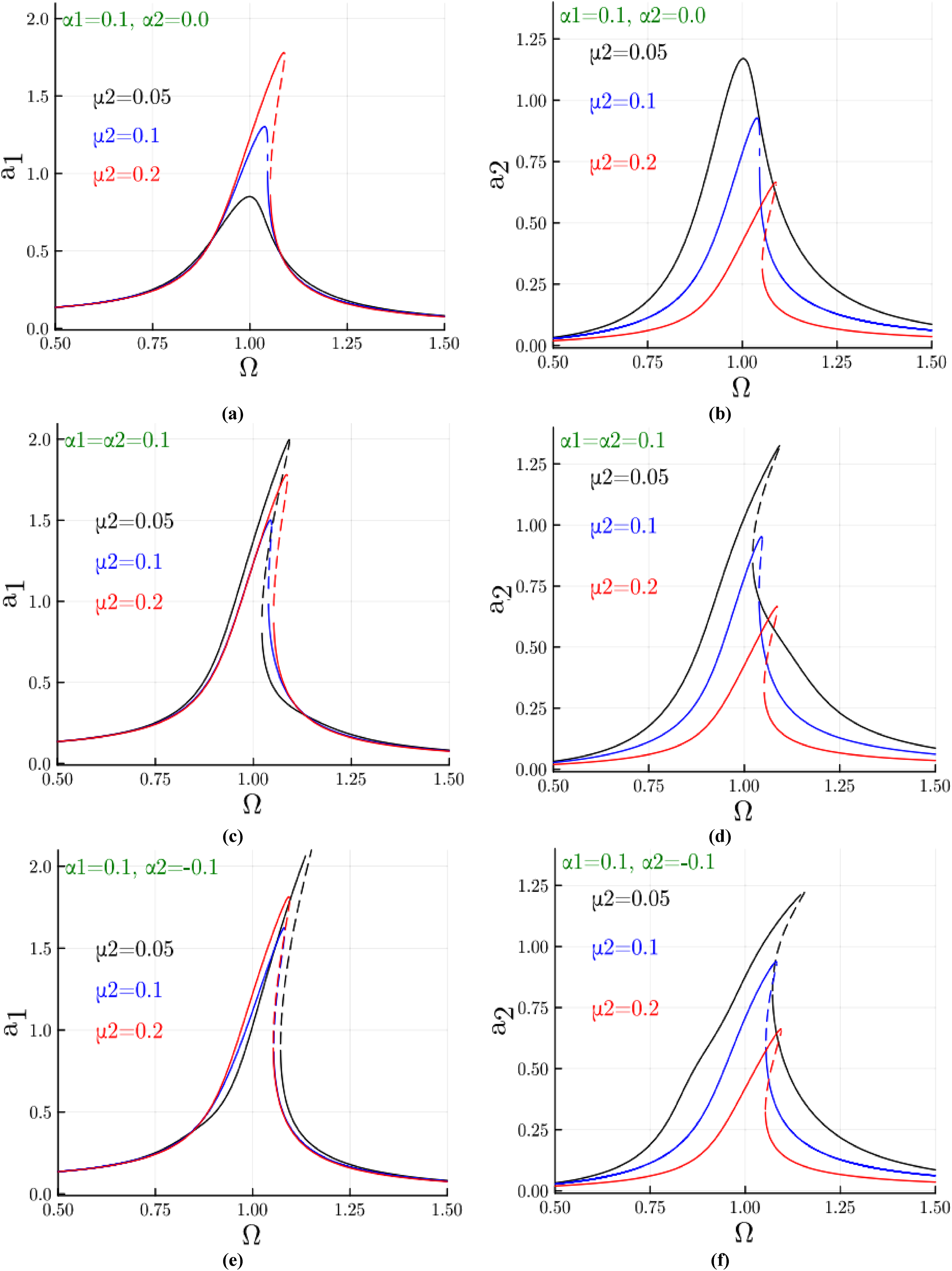
The evolution of $a_1$ and $a_2$ with respect to $\mathrm{\Omega }$ for different values of the mass ratio ( $M_R$ ), Cart-1 damping coefficient ( ${\mu }_1$ ), and Cart-2 damping coefficient ( ${\mu }_2$ ) is illustrated in Figures 14–16, respectively, for ${\alpha }_2=0.1,0.0,$ and $-0.1$ . Figures 14(a) and 14(b) clearly show that Cart-2 acts as a linear vibration absorber, where an increase in the mass ratio broadens the vibration mitigation band for ${\alpha }_2=0.0$ . Conversely, Figure 14(c) through 14(e) demonstrate that Cart-1 behaves as an SDF system, emphasizing the negligible influence of Cart-2 on Cart-1’s dynamic response when ${\alpha }_2\ne 0.0$ . This behavior highlights the minimal interaction between the two carts under these conditions. Figure 14(d) to 14(f) further reveal the amplitude response ( $a_2$ ) of Cart-2, showcasing the complex dynamics of the Cart-2 subsystem. This response reflects interactions between the two modes, giving rise to nonlinear phenomena such as secondary resonances and bifurcations.

Figure 14.

2-DOF cart model oscillation amplitudes against $\mathrm{\Omega }$ for different levels of the mass ratio $M_R=m_2/m_1$ : (a, b) when ${\alpha }_2=0.1$ , (c, d) when ${\alpha }_2=0.0$ , and (e, f) when ${\alpha }_2=-0.1$ .

Figure 15.

2-DOF cart model oscillation amplitudes against $\mathrm{\Omega }$ for different levels of the Cart-1 damping ${\mu }_1$ : (a, b) when ${\alpha }_2=0.1$ , (c, d) when ${\alpha }_2=0.0$ , and (e, f) when ${\alpha }_2=-0.1$ .

Figure 16.

2-DOF cart model oscillation amplitudes against $\mathrm{\Omega }$ for different levels of the Cart-2 damping ${\mu }_2$ : (a, b) when ${\alpha }_2=0.1$ , (c, d) when ${\alpha }_2=0.0$ , and (e, f) when ${\alpha }_2=-0.1$ .

The impact of Cart-1 damping ( ${\mu }_1$ ) on the system’s overall response is presented in Figure 15, where $a_1$ and $a_2$ are plotted against $\mathrm{\Omega }$ ${\mu }_1=0.05,0.1,$ and $0.2$ under varying nonlinear stiffness coefficients ( ${\alpha }_2$ ). Figures 15(a) and 15(b) illustrate the full coupling between the two oscillation modes when ${\alpha }_2=0.0$ . In this case, increasing ${\mu }_1$ reduces the oscillation amplitudes of the coupled system and suppresses the dominance of nonlinear effects. In contrast, Figure 15(c) through 15(f) show that increasing ${\mu }_1$ locally reduces the oscillation amplitude of Cart-1, with minimal impact on Cart-2’s oscillation mode for ${\alpha }_2\ne 0.0$ .

Finally, the evolution of $a_1$ and $a_2$ against $\mathrm{\Omega }$ for varying values of Cart-2 damping ( ${\mu }_2$ ) is displayed in Figure 16. Figures 16(a) and 16(b) illustrate the full coupling between the two subsystems for ${\alpha }_2=0.0$ , where increasing ${\mu }_2$ reduces $a_2$ , thereby increasing $a_1$ . In contrast, Figure 16(c) through 16(f) demonstrate semi-decoupling of the oscillation modes for ${\alpha }_2\ne 0.0$ . Under these conditions, increasing ${\mu }_2$ locally reduces $a_2$ with negligible impact on $a_1$ .

Homotopy perturbation technique versus multiple time-scale analysis

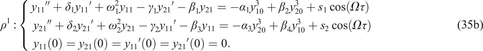
In this section, an analytical approximate solution is derived using the homotopy perturbation technique (HPT) ⁴² for the normalized equations of motion governing the dynamics of the 2-DOF cart model, as presented in equations (7a) and (7b). To facilitate the application of HPT, these equations have been reformulated into a simplified form as follows:

${y_1}^{″}+{\delta }_1{y_1}^{\prime }+{\omega }_1^2{y}_1+{\alpha }_1{y}_1^3-{\gamma }_1{y_2}^{\prime }-{\beta }_1{y}_2-{\beta }_2{y}_2^3=s_1\hspace{0.17em}\cos \left(\Omega \tau \right)$

(30a)

${y_2}^{″}+{\delta }_2{y_2}^{\prime }+{\omega }_2^2{y}_2+{\alpha }_3{y}_2^3-{\gamma }_2{y_1}^{\prime }-{\beta }_3{y}_1-{\beta }_4{y}_1^3=s_2\hspace{0.17em}\cos \left(\Omega \tau \right)$

(30b)

where ${\delta }_1=\frac{{\mu }_1}{\sqrt{\left(1+M_R\hspace{0.17em}{\sin }^2\left(\theta \right)\right)}},$ ${\delta }_2=\frac{\left(1+M_R\right){\mu }_2}{M_R\sqrt{1+M_R\hspace{0.17em}{\sin }^2\left(\theta \right)}},{\alpha }_3=\left(1+\frac{1}{M_R}\right){\alpha }_2,s_1=F,s_2=-Fcos\left(\theta \right)$ . Following the HPT,^42,48 the nonlinear dynamical system described by equations (30a) and (30b) can be expressed as follows:

$H\left(q,\rho \right)=L\left(q\right)+\rho N\left(q\right)-f\left(r\right)=0,\rho \in \left[0,1\right]$

(31)

Here, $L$ and $N$ represent the linear and nonlinear differential operators, respectively, $f\left(r\right)$ is a known analytical function, and $\rho$ denotes the artificially embedded homotopy parameter. Accordingly, the solution of equation (31) can be expressed as a power series in $\rho$ , as follows:

$q=q_0+\rho q_1+{\rho }^2{q}_2+{\rho }^3{q}_3+...$

(32)

In this approach, when $\rho \to 1$ , equation (32) yields the approximate solution to the original (unperturbed) form of equation (31). Therefore, equations (30a) and (30b) can be modified accordingly as follows:

${y_1}^{″}+{\delta }_1{y_1}^{\prime }+{\omega }_1^2{y}_1-{\gamma }_1{y_2}^{\prime }-{\beta }_1{y}_2+\rho \left[{\alpha }_1{y}_1^3-{\beta }_2{y}_2^3-s_1\hspace{0.17em}\cos \left(\Omega \tau \right)\right]=0$

(33a)

${y_2}^{″}+{\delta }_2{y_2}^{\prime }+{\omega }_2^2{y}_2-{\gamma }_2{y_1}^{\prime }-{\beta }_3{y}_1+\rho \left[{\alpha }_3{y}_2^3-{\beta }_4{y}_1^3-s_2\hspace{0.17em}\cos \left(\Omega \tau \right)\right]=0$

(33b)

The solution of equations (33a) and (33b) can be expressed as a power series in the homotopy parameter $\rho$ , as follows:

$y_1=y_{10}+\rho y_{11}+{\rho }^2{y}_{12}+...$

(34a)

$y_2=y_{20}+\rho y_{21}+{\rho }^2{y}_{22}+...$

(34b)

By substituting equations (34a) and (34b) into equations (33a) and (33b), and equating the coefficients of like powers of ${\rho }^0$ and ${\rho }^1$ , we obtain:

${\rho }^0:\{\begin{array}{l}{y_{10}}^{″}+{\delta }_1{y_{10}}^{\prime }+{\omega }_1^2{y}_{10}-{\gamma }_1{y_{20}}^{\prime }-{\beta }_1{y}_{20}=0,\\ \begin{array}{l}{y_{20}}^{″}+{\delta }_2{y_{20}}^{\prime }+{\omega }_2^2{y}_{20}-{\gamma }_2{y_{10}}^{\prime }-{\beta }_3{y}_{10}=0,\\ y_{10}\left(0\right)=A_0,y_{20}\left(0\right)=B_0,{y_{10}}^{\prime }\left(0\right)={y_{20}}^{\prime }\left(0\right)=0.\end{array}\end{array}$

(35a)

${\rho }^1:\{\begin{array}{l}{y_{11}}^{″}+{\delta }_1{y_{11}}^{\prime }+{\omega }_1^2{y}_{11}-{\gamma }_1{y_{21}}^{\prime }-{\beta }_1{y}_{21}=-{\alpha }_1{y}_{10}^3+{\beta }_2{y}_{20}^3+s_1\hspace{0.17em}\cos \left(\Omega \tau \right)\hspace{0.17em}\\ \begin{array}{l}{y_{21}}^{″}+{\delta }_2{y_{21}}^{\prime }+{\omega }_2^2{y}_{21}-{\gamma }_2{y_{11}}^{\prime }-{\beta }_3{y}_{11}=-{\alpha }_3{y}_{20}^3+{\beta }_4{y}_{10}^3+s_2\hspace{0.17em}\cos \left(\Omega \tau \right)\\ y_{11}\left(0\right)=y_{21}\left(0\right)={y_{11}}^{\prime }\left(0\right)={y_{21}}^{\prime }\left(0\right)=0.\end{array}\end{array}$

(35b)

To obtain an analytical solution for equation (35a), the system parameters are selected such that $F=0.03,{\omega }_1=1.1,{\omega }_2=\mathrm{\Omega }=1.0,{\mu }_1=0.5,{\mu }_2=0.23,{\alpha }_1=\frac{\pi }{6},{\alpha }_2=\frac{\pi }{4},M_R=3,$ and $\theta =0$ , accordingly, ${\delta }_1=0.5$ , ${\delta }_2=0.31$ , ${\alpha }_3=\frac{\pi }{3}$ , $s_1=0.03$ , and $s_2=-0.\hspace{0.17em}03$ . In addition, the arbitrary initial conditions $A_0$ and $B_0$ are selected such that $A_0=0.1,B_0=0.2$ . The solutions of equation (35a) are given as follows:

$y_{10}\left(\tau )=-0.029{\mathrm{e}}^{-0.406\tau }(-4.516{\mathrm{e}}^{0.383\tau }\hspace{0.17em}\cos \left(0.481\tau \right)+{\mathrm{e}}^{0.023\tau }\hspace{0.17em}\cos \left(1.355\tau \right)-0.462{\mathrm{e}}^{0.383\tau }\hspace{0.17em}\sin \left(0.481\tau \right)+0.371{\mathrm{e}}^{0.023\tau }\hspace{0.17em}\sin \left(1.355\tau \right)\right)$

(36a)

$y_{20}\left(\tau \right)=0.030{\mathrm{e}}^{-3.619\tau }\left(7.398\times {10}^{-16}{\mathrm{e}}^{0.405\tau }+5.664{\mathrm{e}}^{3.597\tau }\hspace{0.17em}\cos \left(0.481\tau \right)+{\mathrm{e}}^{3.237\tau }\hspace{0.17em}\cos \left(1.355\tau \right)+0.166{\mathrm{e}}^{3.597\tau }\hspace{0.17em}\sin \left(0.481\tau \right)+0.319{\mathrm{e}}^{3.237\tau }\hspace{0.17em}\sin \left(1.355\tau \right)\right)$

(36b)

By substituting equations (36a) and (36b) into the right-hand side of equation (35b) and solving the resulting linear differential equation, analytical expressions for $y_{11}$ and $y_{21}$ can be obtained. Then, by letting $\rho \to 1$ , the first-order approximate solution of equations (30a) and (30b) is given as follows:

$y_1=y_{10}+y_{11}$

(37a)

$y_2=y_{20}+y_{21}$

(37b)

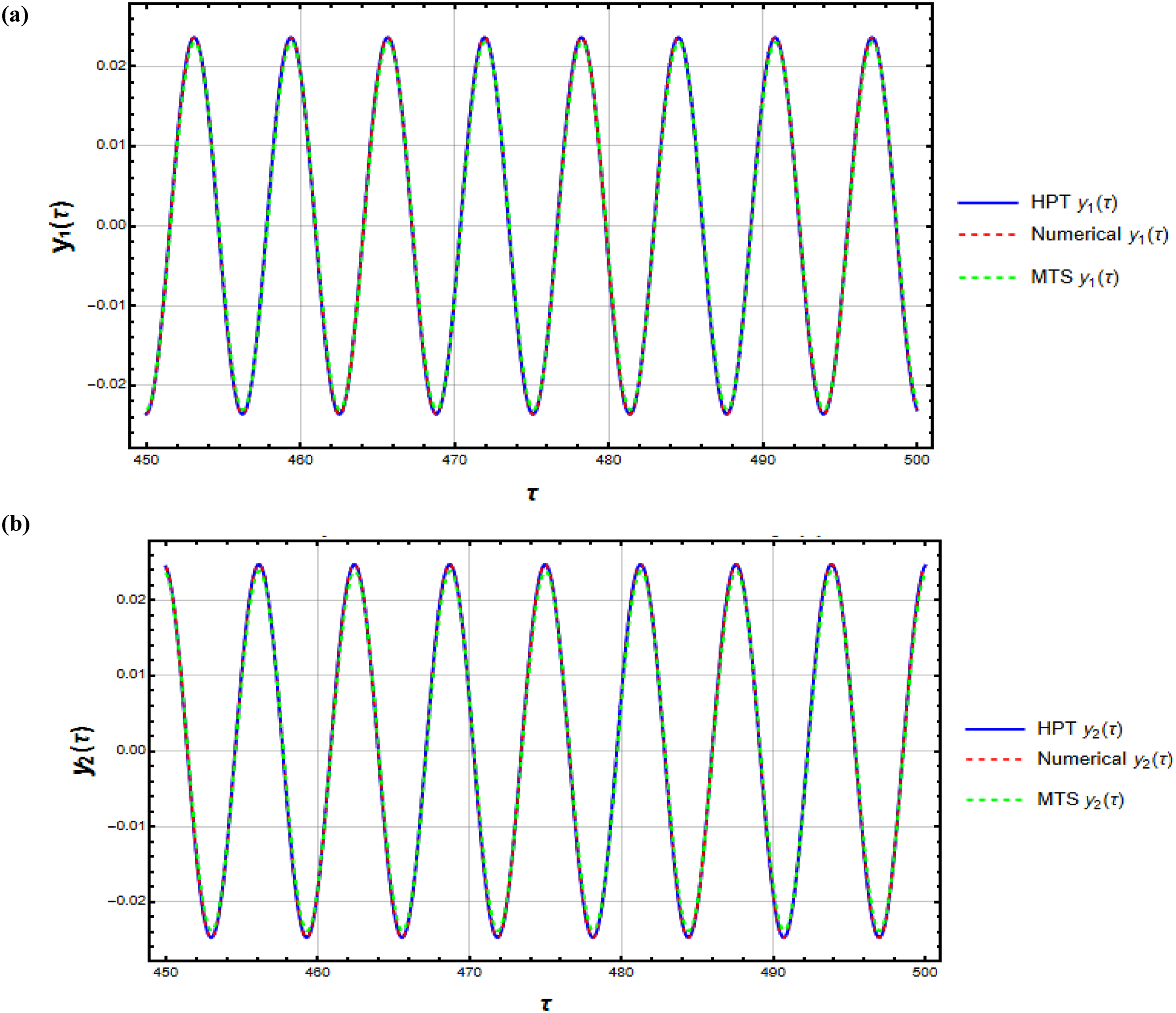
Due to the complexity and length of the expressions, the explicit forms of $y_{11}$ and $y_{21}$ are not presented here. To evaluate the accuracy and reliability of both HPT and MTS methods in analyzing the dynamics of the considered 2-DOF cart model, the system’s time response has been plotted. This comparison includes the HPT-based solution from equations (37a) and (37b), the MTS solution governed by equations (22a) to (23b), and the numerical solution obtained using the Runge-Kutta method, as illustrated in Figure 17. The figure demonstrates strong agreement among the three solution techniques, confirming their validity. In conclusion, while the HPT effectively captures the time-domain behavior of the system with high accuracy, the MTS approach offers a simpler and more flexible framework for analyzing the system’s frequency response characteristics.

Figure 17.

Time histories of $y_1\left(\tau \right)$ and $y_2\left(\tau \right)$ obtained using the homotopy perturbation technique (HPT), the multiple time-scale (MTS) method, and the Runge-Kutta numerical solution.

Conclusion

This work examines the nonlinear dynamics of a 2-DOF cart model oscillating on an inclined surface, comprising Cart-1, a hard-spring Duffing oscillator under near-resonant excitation, and Cart-2, another Duffing oscillator with hardening or softening springs. Using Lagrange’s equations, the normalized equations of motion are derived, and the slow-flow dynamics governing amplitudes and phases are analyzed via multiple time-scale techniques. The evolution of oscillation amplitudes is explored using the continuation method, revealing diverse response patterns. Numerical validation is conducted through Poincaré maps, bifurcation diagrams, basins of attraction, 0–1 chaos tests, and stability charts, ensuring accuracy. Based on the analysis, the following points have been concluded:

(1) The 2-DOF cart system demonstrates six distinct oscillation modes: monostable, bistable, and tristable periodic solutions; period-n solution; a mono-quasiperiodic solution; and the coexistence of periodic and quasiperiodic solutions.

(2) Cart-2 effectively acts as a linear vibration absorber when coupled linearly with Cart-1, mitigating its oscillation amplitudes by establishing an energy exchange mechanism.

(3) The softening nonlinear stiffness coupling between Cart-1 and Cart-2 leads to unbounded oscillations, which pose a significant risk to the stability and safety of the system.

(4) The inclination angle influences the interaction between the carts. At specific angles, such as horizontal alignment, full coupling is observed, enabling Cart-2 to act as a vibration absorber. At other angles, partial decoupling occurs, and Cart-1 behaves as an independent SDF system.

(5) The interaction between Cart-1 and Cart-2 results in localized and coupled oscillation modes, depending on the coupling parameters and inclination angle.

(6) The system exhibits bistable and tristable oscillation modes, with multiple stable solutions coexisting within the same parameter space, governed by initial conditions and excitation parameters.

(7) The system’s oscillation amplitudes and modes are highly dependent on the excitation frequency and force levels, showcasing transitions between localized and coupled behaviors.

(8) The study provides insights into the coupled system’s dynamic behavior under varying excitation conditions, especially in transportation systems.

(9) While the homotopy perturbation technique effectively captures the time-domain behavior of the system with high accuracy, the multiple time-scale approach offers a simpler and more flexible framework for analyzing the system’s frequency response characteristics.