Sage Journals: Discover world-class research

Abstract

In the field of active noise control systems, combining multiple algorithms to improve equalization performance has generated notable interest. Nevertheless, the computation of threshold control parameters for algorithm switching during each iteration leads to a significant increase in computational complexity. Additionally, the frequent switching of algorithms poses challenges in fully leveraging the performance of individual algorithms. Therefore, this paper utilizes the film editing concept to introduce the Algorithm Editing Method (AEM). AEM entails selecting appropriate algorithms based on distinctive iteration stages, followed by precise cutting and splicing according to the defined switching coefficient. Appropriate algorithms are implemented at specific iteration stages, eliminating the requirement for frequent algorithm switching during the iterative process. To substantiate the effectiveness of this approach, the FxLMS and Momentum-FxLMS algorithms serve as foundational components of AEM, enhancing convergence performance in an active noise control system. The results show a noteworthy enhancement in convergence speed and reduction of steady-state error, attained without a simultaneous escalation in computational complexity. Additionally, this study extends the application of AEM to improve the system’s robustness against impulse signals. The simulations and tests results demonstrate the method’s effectiveness, achieving a balance of optimized convergence speed, reduction in steady-state error, and minimized computational complexity.

Keywords

Active noise control adaptive filter algorithm editing method combination algorithm

Introduction

Active noise control (ANC) systems are essential methods for noise control and have wide applicability.^1–5 The adaptive algorithm serves as the core of this system, and its implementation is significantly influenced by the computational cost. Therefore, after years of development, the filtered-x least mean square (FxLMS) algorithm has become the cornerstone algorithm used in the field of ANC due to its computational efficiency, simple structure, and easy implementation.^6–11 However, the FxLMS algorithm’s relatively slow convergence speed under identical convergence criteria is a drawback.^12–14

One potential improvement strategy for addressing this concern is to utilize non-FxLMS techniques. For instance, research conducted by literature¹⁵ introduced the FxOWRLS algorithm with optimized weights, which aims to lower the coefficient upgrade ratio during the iterative process in order to reduce computational costs. Additionally, literature¹⁶ proposed the introduction of the filtered-x maximum correntropy criterion with conjugate gradient (FxMCC-CG) algorithm, which resulted in a notable enhancement of the algorithm’s convergence speed and robustness. Literature¹⁷ presented a new logarithmic loss function that considers the communication error of the residual signal. In addition, Literature¹⁸ proposed a filtered-s Bessel CG (FsBCG)-I algorithm using a functional link artificial neural network as a controller. Literature¹⁹ puts forth an ANC technique based on the FxAPLEHS algorithm. Additionally, the CSS-FxAPLEHS algorithm is proposed as a means of enhancing noise reduction performance. The proposed algorithm provides enhanced robust ANC performance. Literature²⁰ presents a novel hybrid active noise control (ANC, HANC) system, comprising an online secondary path modeling (OSPM) subsystem for input power control. Finally, in literature,²¹ a novel version of the FXAPL algorithm based on nearest Kronecker product decomposition was introduced. While these improved algorithms show promising results by increasing convergence speed and reducing steady-state error, it is important to note that these advancements come with a significant increase in computational complexity.

One possible approach to improve the convergence performance of the algorithm while keeping computational complexity low is to expand upon the FxLMS algorithm. In the literature, the normalized FxLMS algorithm (NFXLMS) has been utilized as a means to eliminate system deviation resulting from Gaussian noise interfering with the ANC system via the computation of a supplemental vector.²² Also proposed in literature is the robust filtered-x normalized least mean square sign algorithm (R-FxNLMSS), which maintains stability under various conditions.²³ This algorithm utilizes the Euclidean norm of the sum of the iterated weight vector and the current weight vector to perform the upgrade iteration of the filter. A simplified scheme for variable step-size filtered-x least mean square (SVSS-FXLMS) was proposed to conduct a thorough statistical analysis of a typical narrowband ANC system.²⁴ In addition, literature²⁵ introduced a novel algorithm for adaptive step-size FxLMS using a reference signal smoothing processor (NASFSxLMS) to expedite the convergence rate and mitigate the impact of outliers. A modal-FxLMS algorithm was introduced in the literature²⁶ for reducing the overall noise level in vibro-acoustic cavities. Similarly, in literature,²⁷ a FxLMS algorithm was proposed with a variable step size to enhance the convergence of the ANC system. The algorithm is based on the arctangent function for updating the step size. Although the computational complexity of these algorithms has decreased in comparison to earlier approaches that use non-FxLMS techniques, it remains decidedly greater than that of the FxLMS algorithm. The literature describes a revised rendition of the FxLMS algorithm, referred to as the Momentum-FxLMS algorithm (M-FxLMS).²⁸ While taking into account the momentum term during the weight coefficient iteration equation, this algorithm retains a computational complexity similar to that of the original FxLMS algorithm. This modification catalyzed the creation and integration of multiple algorithms constructed on the M-FxLMS framework.^29,30 While the M-FxLMS accelerates convergence without elevating computational complexity, it does result in a rise in steady-state error.

Balancing computational complexity, convergence speed, and steady-state error presents a significant challenge when relying solely on a single algorithm. Therefore, the concept of combination algorithms is proposed and applied. For instance, literature proposes the convex combination of the filtered-x maximum versoria criterion (FxMVC) algorithm and FxLMS algorithm³¹ as an example. A technique utilizing the convex combination of two normalized filtered-s least mean square algorithms (CNFSLMS) was proposed for nonlinear ANC systems in previous literature.³² Another study³³ implemented the convex combination of an adaptive filter algorithm in a hearing aid system with a singular microphone and speaker to eliminate sound feedback signals. While combination algorithms can achieve balance in performance, the high computational complexity persists due to the necessity of calculating threshold control parameters for algorithm switching during each iteration. Additionally, the frequent switching of algorithms poses challenges in fully leveraging the performance of individual algorithms.

To address the aforementioned issues, this paper presents the Algorithm Editing Method (AEM), which employs the concept of film editing. AEM selects appropriate algorithms based on the characteristics of different iteration stages, precisely cuts and splices them according to the defined switching coefficient, and utilizes them in specific iteration stages. This approach eliminates the need for frequent algorithm switching throughout the iterative process. By using the switch coefficient as the trigger parameter instead of the threshold control parameter, the computation complexity is increased minimally. It acts as an editing method, allowing for the combination of multiple algorithms or multi-segment algorithms without requiring compatibility assessment.

In this paper, the FxLMS and M-FxLMS algorithms are utilized as fundamental constituents of AEM to improve convergence performance in an active noise control system. The results indicate noteworthy enhancements in convergence speed and reduction of steady-state error, accomplished without any simultaneous increase in computational complexity. Additionally, this paper extends the application of AEM to improve the system’s robustness to impulsive signals. The effectiveness of the method is evident from both simulation and testing results. The paper is organized as follows: the first section provides an introduction to the background and literature review, while the second section presents the analysis and theoretical derivation of AEM. The third section covers the analysis of computational complexity and simulation of convergence performance. The fourth section demonstrates the method’s effectiveness in handling impulse noise and enhancing convergence performance through experiments. The paper concludes in the fifth section.

Development of the algorithm editing method (AEM)

Description of ANC system

The diagram in Figure 1 displays the block diagram of an adaptive single-channel feed-forward ANC system. The feedforward reference signal is denoted by $x (n)$ , while $P (z)$ represents the transfer function of the primary path. $d (n)$ represents the primary noise that’s canceled, and $S (z)$ denotes the transfer function of the secondary path. $W (z)$ is the ANC controller, or adaptive filter. Its output is represented by $y (n)$ , and $y^{'} (n)$ is the secondary noise used to counteract the primary noise. The transfer function for phase compensation is represented by $\hat{S} (z)$ , which can be acquired through adaptive filtering via either offline or online estimation methods.³⁴ Lastly, the residual error is denoted by $e (n)$ .

Figure 1.

Block diagram of a single-channel ANC system.

The adaptive filter output signal $y (n)$ is given by

y (n) = W^{T} (n) X (n)

(1)

where the reference signal vector is denoted by

X (n) = {[x (n), x (n - 1), \dots, x (n - L + 1)]}^{T}

, the order length of the filter is represented by

L

,and the weight vector of the adaptive filter is denoted by

W (n) = {[w_{0} (n), w_{1} (n), \dots, w_{L - 1} (n)]}^{T}

. The residual error can be calculated by

e (n) = d (n) - y^{'} (n)

(2)

d (n) = x (n) * p (n)

(3)

y^{'} (n) = y (n) * s (n)

(4)

where

s (n)

and

p (n)

are the impulse responses of

S (z)

and

P (z)

, respectively,

*

represents the convolution operator.

The filtered-x least mean square (FxLMS) algorithm

The cost function for the FxLMS algorithm is expressed by the following equation

J (n) = E [e^{2} (n)] = E {{[d (n) - W^{T} (n) X (n) * s (n)]}^{2}}

(5)

The loss function $J (n)$ is a quadratic function with respect to the weight vector $W (n)$ , and the weight vector derivation equation can be obtained³⁵

W (n + 1) = W (n) - μ Δ J = W (n) + μ e (n) [s (n) * X (n)]

(6)

The iterative process can be analogized to a ball rolling down a multidimensional bowl-shaped surface, as shown in Figure 2. The main objective of optimization is to quickly stabilize the ball at the bottom of the “bowl.” The FxLMS algorithm utilizes a constant step size, designated as $μ$ , when iterating the weight coefficient vector $W (n)$ . This implies that the iterative process does not take into consideration the impact of the slope along the “bowl” wall. Regardless of the ball’s position on the bowl wall, it uniformly advances towards the bottom with consistent increments. Hence, the value of $μ$ determines the balance between the algorithm’s steady-state error and its convergence speed. Opting for a higher value of $μ$ speeds up convergence, but this also causes oscillations at the base of the basin and increases the steady-state error. Choosing a smaller value reduces the steady-state error, but significantly slows down convergence speed.

Figure 2.

Iterative process of the weight vector.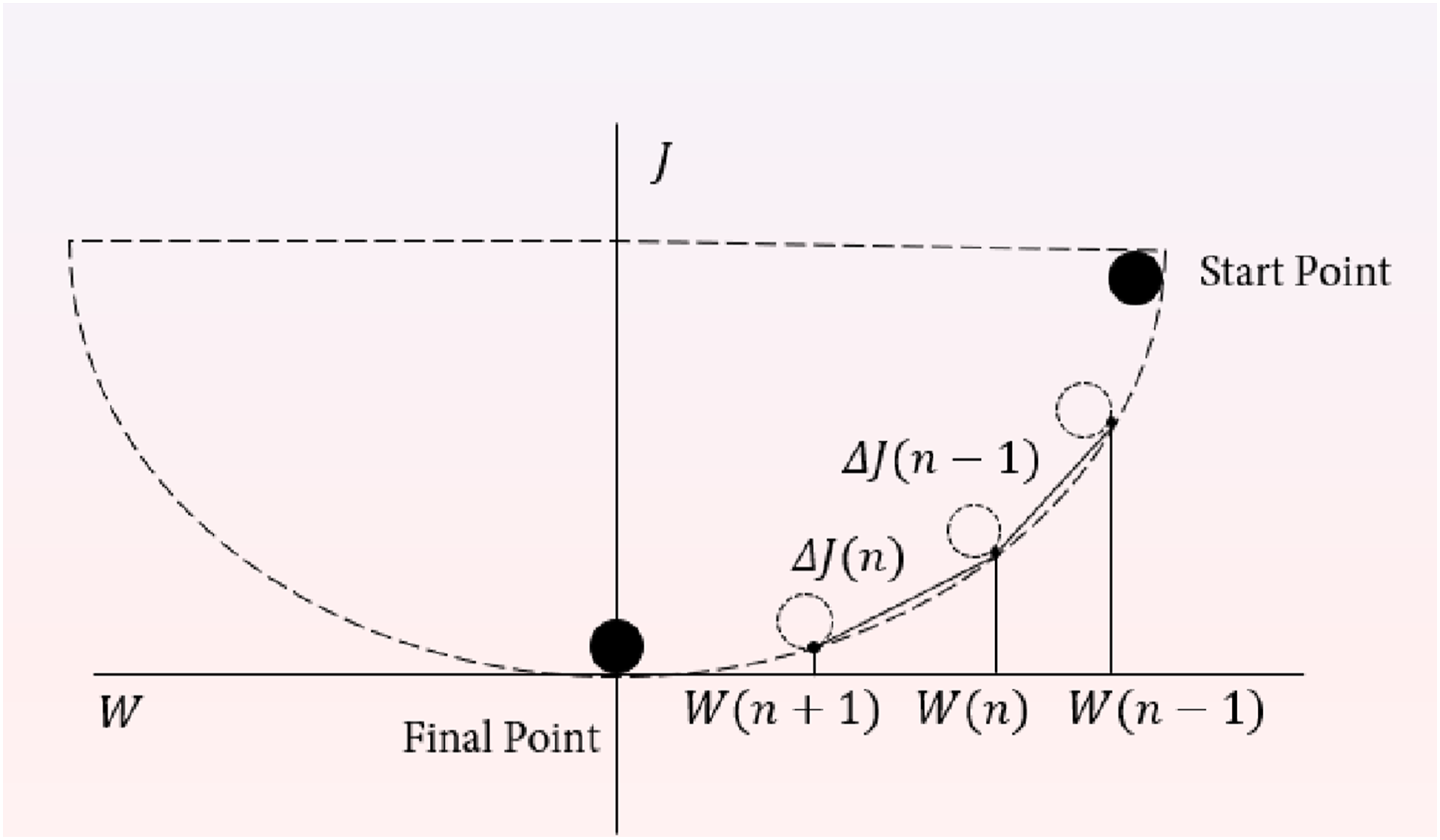

The momentum FxLMS (M-FxLMS) algorithm

The weight vector derivation equation for M-FxLMS algorithm can be obtained³⁶

W (n + 1) = W (n) + μ e (n) [s (n) * X (n)] + p [W (n) - W (n - 1)]

(7)

The momentum term $W (n) - W (n - 1)$ and coefficient $p$ are essential factors in adjusting the iterative weight coefficient based on the previous iteration. This principle can be likened to introducing inertia, where a ball moves on a curved surface of a bowl, taking into account how bowl slope affects iteration. In steeper sections, the ball gains momentum, thereby accelerating its descent, while in gentler parts, the ball’s descent slows.

The algorithm editing method (AEM)

In order to facilitate a comparison of the convergence performance of the aforementioned algorithms, it is necessary to take $X^{'} (n) = s (n) * X (n)$ and rewrite the weight vector iteration formula of the momentum FxLMS algorithm in the following form

W (n + 1) - W (n) = p [W (n) - W (n - 1)] + 2 μ e (n) [X^{'} (n)]

(8)

The weight error fitness is defined as $V (n) = W (n) - W_{*}$ , $W_{*} = R^{- 1} P$ denotes the converged Wiener solution of the algorithm $R = E [X^{'} (n) {X^{'}}^{T} (n)]$ , $P = E [X^{'} (n) d (n)]$ , and $Ε [\cdot]$ denotes the expectation operator. The above equation can thus be rewritten in the following form

\begin{array}{l} V (n + 1) - V (n) = p [V (n) - V (n - 1)] + 2 μ e_{*} (n) X^{'} (n) \\ \begin{array}{l} \begin{array}{l} \begin{array}{l} - \end{array} 2 \end{array} \end{array} μ X^{'} (n) {X^{'}}^{T} (n) V (n) \end{array}

(9)

e_{*} (n) = d (n) - {W_{*}}^{T} X^{'} (n)

represents the output residual when the algorithm reaches convergence.

R = Q Λ Q^{T}

Λ = d i a g [λ_{1}, λ_{2}, \dots λ_{n}]

Q Q^{T} = I

\tilde{V} (n) = Q^{T} V (n)

. The above equation can then be rewritten as

\begin{array}{l} \tilde{V} (n + 1) - \tilde{V} (n) = p [\tilde{V} (n) - \tilde{V} (n - 1)] + 2 μ e_{*} (n) \tilde{X^{'}} (n) \\ \begin{array}{l} \begin{array}{l} \begin{array}{l} - \end{array} 2 \end{array} \end{array} μ \tilde{X^{'}} (n) {\tilde{X^{'}}}^{T} (n) \tilde{V} (n) \end{array}

(10)

\tilde{X^{'}} (n) = Q^{T} X^{'} (n)

, given that

e_{*} (n)

is orthogonal to

\tilde{X^{'}} (n)

, it follows that

E [e_{*} (n) \tilde{X^{'}} (n)] = 0

is also true. The simultaneous computation of the expectation on both sides of the above equation yields

E [\tilde{V} (n + 1) - \tilde{V} (n)] = p E [\tilde{V} (n) - \tilde{V} (n - 1)] - 2 μ Λ E [\tilde{V} (n)]

(11)

A 2N-dimensional state vector can be defined as $\tilde{U} (n + 1) = [\begin{array}{l} \tilde{V} (n + 1) \\ \tilde{V} (n) \end{array}]$ , and the above equation can thus be rewritten as follows

E [\tilde{U} (n + 1)] = [\begin{array}{l} (1 + p) I - 2 μ Λ & - p I \\ I & 0 \end{array}] E [\tilde{U} (n)]

(12)

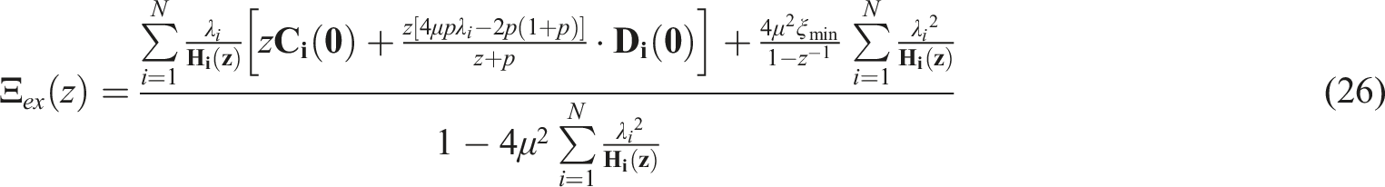
The aforementioned equation demonstrates that the convergence of the algorithm is contingent upon the root of the transfer matrix ${β_{i}}$

\det [\begin{array}{l} (1 + p) I - 2 μ Λ & - p I \\ I & 0 \end{array}] = 0

(13)

The algorithm converges when the condition $| β_{i} | < 1, i = 1, \dots, 2 N$ is satisfied.

A study of the rate of convergence of algorithms

The speed of convergence of the algorithm can be evaluated by calculating the time constant of the weight vectors. The time constant of the ith weight vector iteration of the algorithm can be obtained using the following equation

1 - \frac{1}{τ_{i}} \approx | β_{i} |

(14)

Combining equations (12) and (13) yields

1 - \frac{1}{τ_{i}} \approx \frac{1 + p - 2 μ λ_{i}}{2} . [1 + \sqrt{1 - \frac{4 p}{{(1 + p - 2 μ λ_{i})}^{2}}}]

(15)

In general,

| p | ≪ 1

.It can be demonstrated that the following equation is true

\sqrt{1 - \frac{4 p}{{(1 + p - 2 μ λ_{i})}^{2}}} \approx 1 - \frac{2 p}{{(1 + p - 2 μ λ_{i})}^{2}}

(16)

τ_{i} \approx (\frac{1 + p - 2 μ λ_{i}}{1 + 2 p - 2 μ λ_{i}}) \frac{1}{2 μ λ_{i}}

(17)

In general,

2 μ λ_{i} ≪ 1

. The following equation is therefore true

τ_{i} \approx (\frac{1 + p}{1 + 2 p}) \frac{1}{2 μ λ_{i}}

(18)

Equation (18) represents the time constant of the momentum FxLMS algorithm. It is noteworthy that this equation becomes the time constant of the FxLMS algorithm when $p = 0$ . The time constants of the FxLMS algorithm and the momentum FxLMS algorithm are defined as $τ_{i, F x L M S}$ and $τ_{i, M_F x L M S}$ , respectively. $η (p) = (1 + p) / (1 + 2 p)$ .The relationship between the two time constants is given by

τ_{i, M_F x L M S} = η (p) τ_{i, F x L M S}

(19)

From the above relationship, the momentum FxLMS algorithm has a smaller time constant and converges faster compared to the FxLMS algorithm, since $η (p) < 1 (p \neq 0)$ , and the value of $p$ is proportional to the convergence speed.

A study of the misalignment of algorithms

The misalignment is a measure of the proximity of the adaptive process weight vector to the Wiener solution, and can characterize the accuracy of the convergence of the algorithm, when the misalignment is large, the converged solution will always oscillate around the optimal solution with a large magnitude, in order to analyze the misalignment performance of the two algorithms, the following variables are defined

\begin{array}{l} C_{i} (n + 1) = E {[\tilde{V} (n + 1) {\tilde{V}}^{T} (n + 1)]}_{i, i} \\ D_{i} (n + 1) = E {[\tilde{V} (n + 1) {\tilde{V}}^{T} (n)]}_{i, i} \end{array}

(20)

The minimum mean square error when the algorithm converges to the optimal solution, designated as $ξ_{\min} = E [e_{*}^{2} (n)]$ , can be defined as a Z-transformation of equation (20). This yields the following relation

D_{i} (z) = \frac{(1 + p - 2 μ λ_{i}) C_{i} (z) + z D_{i} (0)}{z + p}

(21)

\begin{array}{l} C_{i} (z) H_{i} (z) = z C_{i} (0) + \frac{4 μ^{2} ξ_{\min} λ_{i}}{1 - z^{- 1}} + \frac{z [4 μ p λ_{i} - 2 p (1 + p)]}{z + p} \\ \begin{array}{l} \begin{array}{l} \cdot \end{array} \end{array} D_{i} (0) + 4 μ^{2} λ_{i} \sum_{j = 1}^{N} λ_{j} C_{j} (z) \end{array}

(22)

\begin{array}{l} H_{i} (z) = z - {(1 + p)}^{2} - p^{2} z^{- 1} - 8 μ^{2} λ_{i}^{2} + 4 μ (1 + p) λ_{i} \\ \begin{array}{l} \begin{array}{l} - \end{array} \frac{(1 + p - 2 μ λ_{i}) [4 μ p λ_{i} - 2 p (1 + p)]}{z + p} \end{array} \end{array}

(23)

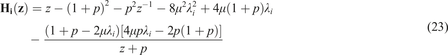
Define the overshooting mean square error as

ξ_{e x} (n) = \sum_{i = 1}^{N} λ_{i} C_{i} (n)

(24)

A Z-transformation of the aforementioned equation yields the following result

Ξ_{e x} (z) = \sum_{i = 1}^{N} λ_{i} C_{i} (z)

(25)

Upon combining the equations (21) through (23) with equation (25), the following result is obtained

Ξ_{e x} (z) = \frac{\sum_{i = 1}^{N} \frac{λ_{i}}{H_{i} (z)} [z C_{i} (0) + \frac{z [4 μ p λ_{i} - 2 p (1 + p)]}{z + p} \cdot D_{i} (0)] + \frac{4 μ^{2} ξ_{\min}}{1 - z^{- 1}} \sum_{i = 1}^{N} \frac{{λ_{i}}^{2}}{H_{i} (z)}}{1 - 4 μ^{2} \sum_{i = 1}^{N} \frac{{λ_{i}}^{2}}{H_{i} (z)}}

(26)

Subsequently, the overshooting mean square error at the point of convergence for the algorithm can be expressed as follows

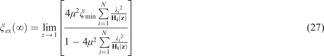
ξ_{e x} (\infty) = \lim_{z \to 1} [\frac{4 μ^{2} ξ_{\min} \sum_{i = 1}^{N} \frac{{λ_{i}}^{2}}{H_{i} (z)}}{1 - 4 μ^{2} \sum_{i = 1}^{N} \frac{{λ_{i}}^{2}}{H_{i} (z)}}]

(27)

The misalignment of algorithms can be quantified as follows

M = ξ_{e x} (\infty) / ξ_{\min}

(28)

In the context of the FxLMS algorithm, the misalignment can be expressed as follows

\begin{array}{l} M_{p} = \frac{K_{p}}{1 - K_{p}} \\ \begin{array}{l} \begin{array}{l} \begin{array}{l} \begin{array}{l} \begin{array}{l} (p \neq 0) \end{array} \end{array} \end{array} \end{array} \end{array} \\ K_{p} = 4 μ^{2} \sum_{i = 1}^{N} \frac{{λ_{i}}^{2}}{\lim_{z \to 1} H_{i} (z)} = \sum_{i = 1}^{N} \frac{μ λ_{i} (1 + p)}{1 - p^{2} - 2 μ λ_{i}} \end{array}

(29)

When

p = 0

, the aforementioned equation is equivalent to the misalignment of the FxLMS algorithm

\begin{array}{l} M_{0} = \frac{K_{0}}{1 - K_{0}} \\ K_{0} = \sum_{i = 1}^{N} \frac{μ λ_{i}}{1 - 2 μ λ_{i}} \end{array}

(30)

In order to facilitate a comparison of the degree of misalignment exhibited by the two algorithms, the relevant data is obtained from equations (29) and (30)

\frac{M_{p} - M_{0}}{M_{0}} = \frac{K_{p} - K_{0}}{K_{0} (1 - K_{p})}

(31)

K_{p} - K_{0} = \sum_{i = 1}^{N} μ λ_{i} (\frac{1 + p}{1 - p^{2} - 2 μ λ_{i}} - \frac{1}{1 - 2 μ λ_{i}})

(32)

Because

| p | ≪ 1

. The aforementioned equation can be reduced to the following form

K_{p} - K_{0} \approx \sum_{i = 1}^{N} \frac{p μ λ_{i}}{1 - 2 μ λ_{i}} = p K_{0}

(33)

Upon bringing equation (33) into equation (31) and considering

2 μ λ_{i} ≪ 1

, it can be demonstrated that equation (31) can be simplified as

\frac{M_{p} - M_{0}}{M_{0}} \approx p

(34)

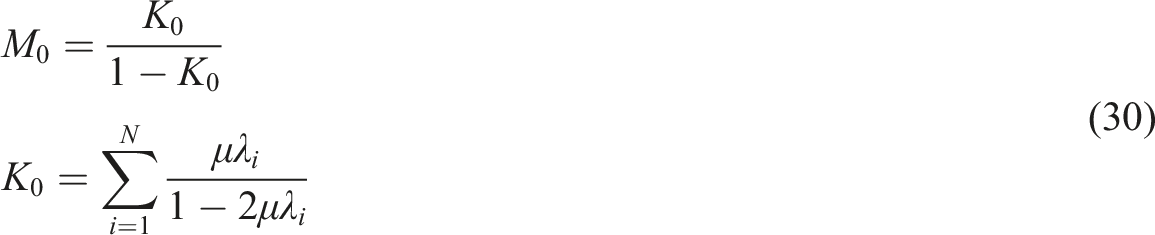
As can be observed from the aforementioned equation, the momentum FxLMS algorithm exhibits a greater degree of misalignment than the FxLMS algorithm. Furthermore, the magnitude of this misalignment is directly proportional to the value of $p$ .

The advantages of the algorithm editing method (AEM)

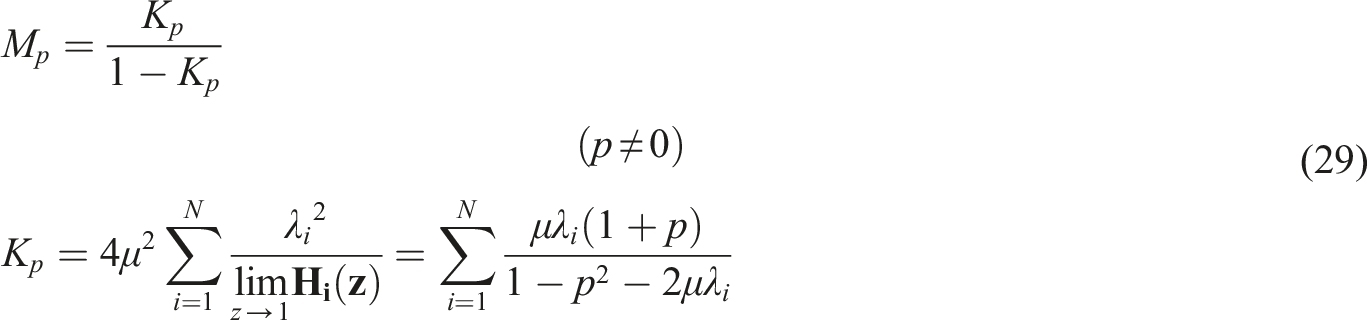
The analysis indicates that the momentum FxLMS algorithm exhibits a faster convergence speed than the FxLMS algorithm. However, it also demonstrates a larger dissonance. The inverse relationship between convergence speed and dissonance suggests that it may be challenging to achieve an optimal balance between these two performance metrics when employing either algorithm in isolation. To address this challenge, in this paper, the algorithm editing method is employed to merge and adapt the two algorithms, segmenting the overall convergence process into two phases. Initially, at the outset of the iteration, the momentum FxLMS algorithm is utilized to achieve a faster iteration speed, with a larger $p$ value. Subsequently, at the conclusion of the iteration, as the algorithm transitions into the convergence interval, the FxLMS algorithm is employed to prevent an excessive dislocated amount, with $= 0$ . This guarantees that the convergence process is completed in the shortest possible time when a specific residual threshold is employed as the convergence target.

In order to analyze the convergence performance of the algorithm editing method, it is assumed that the first iteration represents a dividing line between two distinct phases. Furthermore, it is assumed that the momentum FxLMS algorithm is used when $n < m$ , and the FxLMS algorithm is used when $n > m$ . In this context, the time constant $τ_{i, A E M}$ and the misalignment $M_{A E M}$ of the algorithm editing method can be expressed in the following form

τ_{i, A E M} = \frac{m}{n} τ_{i, M_F x L M S} + \frac{n - m}{n} τ_{i, F x L M S} = (\frac{1 + 2 p}{1 + p} - \frac{m}{n} \cdot \frac{p}{1 + p}) τ_{i, M_F x L M S}

(35)

M_{A E M} = [\frac{m}{n} \cdot (1 + p) + \frac{n - m}{n}] M_{0} = (\frac{n + m p}{n}) M_{0}

(36)

From the aforementioned equation, it can be observed that by modifying the values of the parameters $p$ and $m$ , the time constant of the algorithm editing method can be made to approach that of the momentum FxLMS algorithm as closely as possible. Furthermore, the discrepancy in alignment will converge to the discrepancy observed in the FxLMS algorithm. This implies that the equation can simultaneously consider the convergence speed and the discrepancy in alignment. The algorithm editing method alternates between the two algorithms at a designated point in time to ascertain whether the transition introduces additional disturbances. For illustrative purposes, let us assume that the algorithm switches from the momentum FxLMS algorithm to the FxLMS algorithm at $n = m$ . In this case, the gradient of the weight vector of the algorithm editing method can be expressed as

Δ W (m) = W (m) - W (m - 1) = p [W (m - 1) - W (m - 2)] + 2 μ e (m - 1) [X^{'} (m - 1)]

(37)

Δ W (m + 1) = W (m + 1) - W (m) = 2 μ e (m) [X^{'} (m)]

(38)

Subsequently, the gradient of the weight vector in question, both before and after the algorithm switch, can be obtained

\begin{array}{l} W (m + 1) - W (m - 1) = p [W (m - 1) - W (m - 2)] \\ + 2 μ e (m - 1) [X^{'} (m - 1)] + 2 μ e (m) [X^{'} (m)] \end{array}

(39)

In the absence of the algorithm editing method, the weight vector gradient can be expressed as follows

Δ W (m + 1) = W (m + 1) - W (m) = p [W (m) - W (m - 1)] + 2 μ e (m) [X^{'} (m)]

(40)

In this instance, it is then feasible to obtain

\begin{array}{l} W (m + 1) - W (m - 1) = p [W (m) - W (m - 2)] \\ + 2 μ e (m - 1) [X^{'} (m - 1)] + 2 μ e (m) [X^{'} (m)] \end{array}

(41)

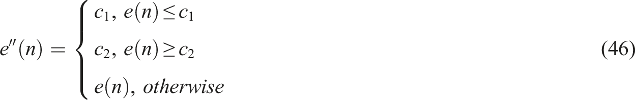
A comparison of equations (39) and (41) reveals that the larger gradient of $W (m) - W (m - 2)$ relative to $W (m - 1) - W (m - 2)$ ensures that the algorithm editing method not only avoids introducing additional shocks during the switching process but also facilitates a smoother iterative process. Nevertheless, as previously discussed, it is of the utmost importance that the method be applied with the utmost attention to detail. 1. The spliced objects should exhibit disparate advantages at different stages of the iterative process. This enables the effect of AEM to be realized through editing. However, if the two objects display greater consistency throughout the iterative process, the AEM method is not applicable. Secondly, to avoid a significant impact when switching between algorithms, it is preferable for the applied objects to belong to the same family of algorithms. This allows for a more seamless switching effect when switching between them. In order to circumvent significant disruptions during the transition between algorithms, it is preferable to utilize algorithms belonging to the same family. This approach enables a more seamless transition, thereby enhancing the efficacy of AEM.

Applications of the algorithm editing method

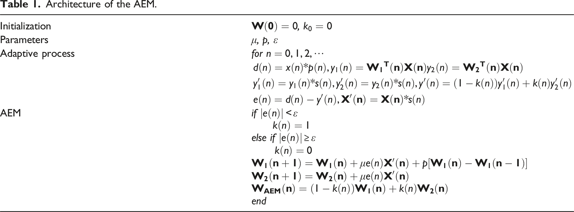
The block diagram of the algorithm editing method is depicted in Figure 3, and a detailed illustration is presented in Table 1.

Figure 3.

Block diagram of the AEM.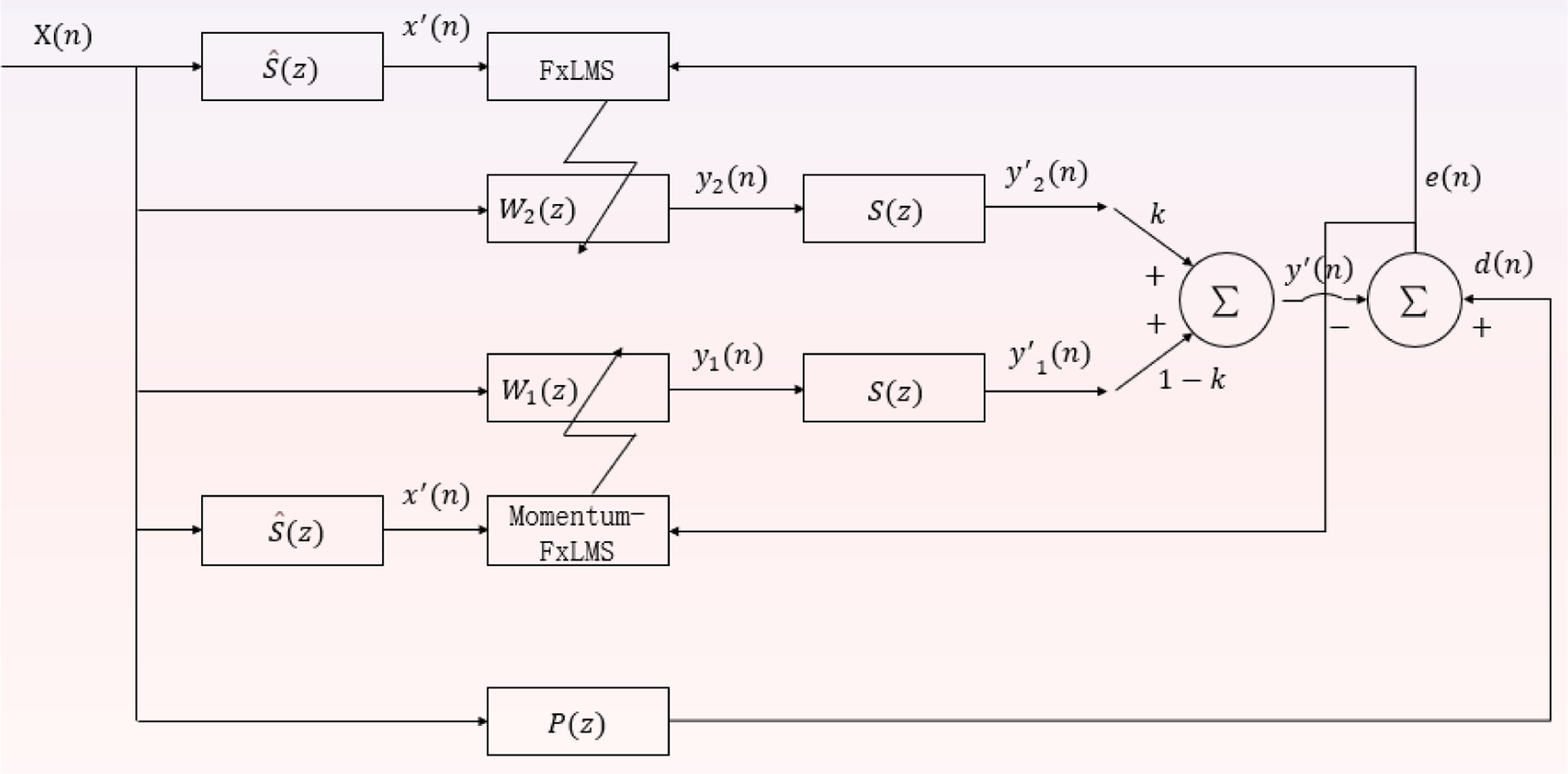

Table 1.

Architecture of the AEM.

Initialization	$W (0) = 0$ , $k_{0} = 0$
Parameters	$μ$ , $p$ , $ε$
Adaptive process	for $n = 0, 1, 2, \dots$
Adaptive process	$\begin{array}{l} d (n) = x (n) * p (n), y_{1} (n) = {W_{1}}^{T} (n) X (n) y_{2} (n) = {W_{2}}^{T} (n) X (n) \\ y_{1}^{'} (n) = y_{1} (n) * s (n), y_{2}^{'} (n) = y_{2} (n) * s (n), y^{'} (n) = (1 - k (n)) y_{1}^{'} (n) + k (n) y_{2}^{'} (n) \\ e (n) = d (n) - y^{'} (n), X^{'} (n) = X (n) * s (n) \end{array}$
AEM	if $\| e (n) \| < ε$
	$k (n) = 1$
	else if $\| e (n) \| \geq ε$
	$k (n) = 0$
	$W_{1} (n + 1) = W_{1} (n) + μ e (n) X^{'} (n) + p [W_{1} (n) - W_{1} (n - 1)]$
	$W_{2} (n + 1) = W_{2} (n) + μ e (n) X^{'} (n)$
	$W_{A E M} (n) = (1 - k (n)) W_{1} (n) + k (n) W_{2} (n)$
	end

The overall output expression of the filter in the Algorithm Editing Method (AEM) can be represented as follows

y^{'} (n) = (1 - k) y_{1}^{'} (n) + k y_{2}^{'} (n)

(42)

To avoid calculating threshold control parameters for algorithm switching in each iteration, the switch coefficient 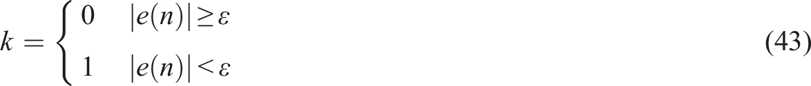$k$ serves as the triggering parameter, rather than the threshold control parameters. Determined by the fixed threshold $ε$ and the residual error $e (n)$ , the switch coefficient takes on a binary value of 0 or 1

k = {\begin{cases} 0 \begin{array}{l} | e (n) | \geq ε \end{array} \\ 1 \begin{array}{l} | e (n) | < ε \end{array} \end{cases}

(43)

The presence of impulse signals poses a significant challenge in the implementation of ANC systems. Aberrant samples, characterized by spikes or disproportionately large values originating from impulse signals, have the potential to induce considerable oscillations in the weight coefficients of the adaptive filter within the algorithm, potentially leading to algorithmic divergence. A series of algorithms have been developed with the aim of enhancing the resilience of ANC impact resistance.^37–39 A literature-referenced approach addressing the mitigation of impulse signals was introduced to enhance the system’s robustness.⁴⁰ Upon surpassing a predefined threshold, the reference signal $x (n)$ undergoes substitution with a value of zero, as illustrated in equation (44)

x^{'} (n) = {\begin{cases} x (n) \\ 0 \end{cases} \begin{array}{l} , i f \begin{array}{l} x (n) \in [c_{1}, c_{2}] \end{array} \\ o t h e r w i s e \end{array}

(44)

The methods described exhibit notable robustness in handling less acute impulse signals, characterized by $α > 1.5$ within a symmetric stable distribution. However, the algorithm’s performance diminishes when faced with more acute and transient signals (e.g., $α < 1.5$ using the same distribution), revealing a notable limitation in adaptability. As an improvement, the literature⁴¹ proposed the substitution of $x (n)$ and $e (n)$ with signal statistics, as exemplified in equations (45) and (46)

x^{″} (n) = {\begin{cases} c_{1}, \begin{array}{l} x (n) \leq c_{1} \end{array} \\ c_{2}, \begin{array}{l} x (n) \geq c_{2} \end{array} \\ x (n), \begin{array}{l} o t h e r w i s e \end{array} \end{cases}

(45)

e^{″} (n) = {\begin{cases} c_{1}, \begin{array}{l} e (n) \leq c_{1} \end{array} \\ c_{2}, \begin{array}{l} e (n) \geq c_{2} \end{array} \\ e (n), \begin{array}{l} o t h e r w i s e \end{array} \end{cases}

(46)

Nonetheless, the algorithm incorporates a virtual threshold signal in lieu of actual impulse signals, thereby introducing a novel form of perturbation. This perturbation amplifies with heightened signal instability. Furthermore, the algorithm’s efficacy is significantly reliant on the judicious selection of the threshold. In response to these challenges, this study leverages the AEM to fortify the algorithm’s resilience against impulsive influences. The core principle entails concurrent monitoring of primary noise

d (n)

, secondary noise

y^{'} (n)

, and residual signal

e (n)

. When impulse signals manifest in any of these signals,

x^{'} (n), d (n), y^{'} (n), e (n), and W (n)

undergo synchronous clipping, proficiently eliminating the impulse signals and mitigating their impact on the algorithm. Furthermore, the iterative process, both pre- and post-clipping, seamlessly integrates to sustain continuity and avert disruption to the iterative procedure. The architecture of the AEM designed to counteract impulse signals is detailed in Table 2.

Table 2.

The architecture of the AEM against impulse signals.

Parameters	$c$
Algorithm scissors	$i f d (n) \geq c o r y^{'} (n) \geq c o r e (n) \geq c, t h e n$
	$d e l x^{'} (n), d e l y^{'} (n), d e l d (n), d e l e (n), d e l W (n)$
	$f o r i = 0, 1, 2, \dots, n - 1$
	$x^{'} (n - i) = x^{'} (n - (i + 1))$
	$y^{'} (n - i) = y^{'} (n - (i + 1))$
	$d (n - i) = d (n - (i + 1))$
	$e (n - i) = e (n - (i + 1))$
	$W (n - i) = W (n - (i + 1))$
	$e n d$
	$x^{'} (0) = 0, y^{'} (0) = 0, d (0) = 0, e (0) = 0, W (0) = 0$
	continue

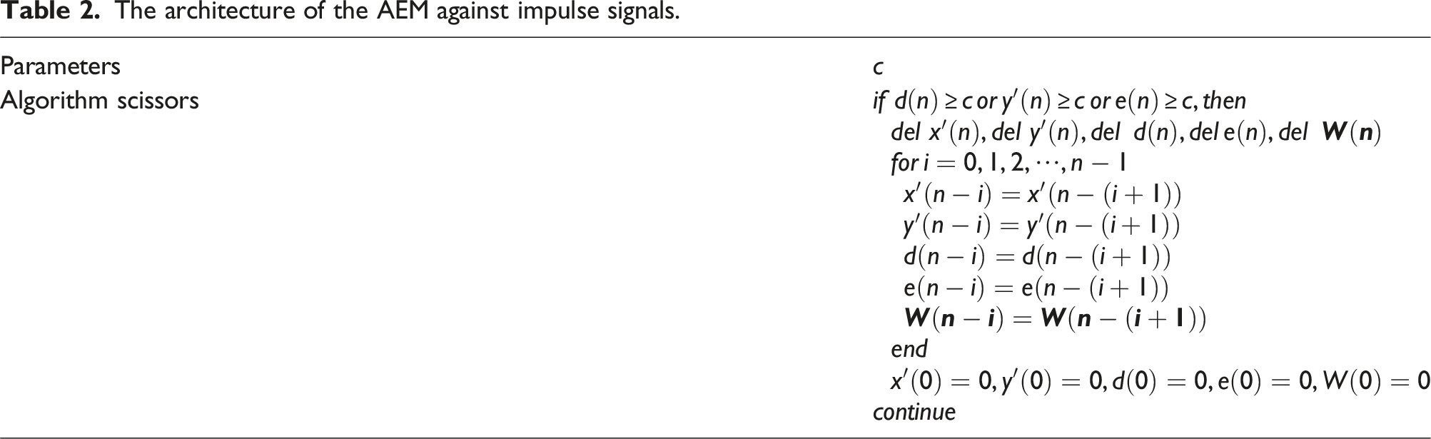
To attenuate the impulse signals via a “clipping” process, the computations are executed in accordance with equation (47) through equation (51)

x^{'} (n) = {\begin{cases} x^{'} (n - 1) \begin{array}{l} & x^{'} (0) = 0 & \begin{array}{l} i f & d (n) \geq c & o r & y^{'} (n) \geq c & o r & e (n) \geq c \end{array} \end{array} \\ x^{'} (n) \begin{array}{l} \begin{array}{l} \begin{array}{l} \begin{array}{l} o t h e r w i s e \end{array} \end{array} \end{array} \end{array} \end{cases}

(47)

y^{'} (n) = {\begin{cases} y^{'} (n - 1) \begin{array}{l} & y^{'} (0) = 0 & \begin{array}{l} i f & d (n) \geq c & o r & y^{'} (n) \geq c & o r & e (n) \geq c \end{array} \end{array} \\ y^{'} (n) \begin{array}{l} \begin{array}{l} \begin{array}{l} \begin{array}{l} o t h e r w i s e \end{array} \end{array} \end{array} \end{array} \end{cases}

(48)

d (n) = {\begin{cases} d (n - 1) \begin{array}{l} & d (0) = 0 & \begin{array}{l} i f & d (n) \geq c & o r & y^{'} (n) \geq c & o r & e (n) \geq c \end{array} \end{array} \\ d (n) \begin{array}{l} \begin{array}{l} \begin{array}{l} \begin{array}{l} o t h e r w i s e \end{array} \end{array} \end{array} \end{array} \end{cases}

(49)

e (n) = {\begin{cases} e (n - 1) \begin{array}{l} & e (0) = 0 & \begin{array}{l} i f & d (n) \geq c & o r & y^{'} (n) \geq c & o r & e (n) \geq c \end{array} \end{array} \\ e (n) \begin{array}{l} \begin{array}{l} \begin{array}{l} \begin{array}{l} o t h e r w i s e \end{array} \end{array} \end{array} \end{array} \end{cases}

(50)

W (n) = {\begin{cases} W (n - 1) \begin{array}{l} & W (0) = 0 & \begin{array}{l} i f & d (n) \geq c & o r & y^{'} (n) \geq c & o r & e (n) \geq c \end{array} \end{array} \\ W (n) \begin{array}{l} \begin{array}{l} \begin{array}{l} \begin{array}{l} o t h e r w i s e \end{array} \end{array} \end{array} \end{array} \end{cases}

(51)

The parameter $c$ serves as a predetermined threshold, signifying a multiple of the average statistical value of the corresponding signal. Any value equal to or exceeding $c$ is recognized as indicative of impulse signals.

Simulation of the performance of the algorithm editing method (AEM)

The convergence performance simulation

To evaluate convergence performance, a 7th-order FIR filter is utilized for the determination of both the primary path transfer function

p (n) = [0.01, 0.25, 0.5, 1, 0.5, 0.25, 0.01]

and the secondary path transfer function

s (n) = p (n) * 0.25

. Assuming

\hat{s} (n) = s (n)

, an adaptive filter vector,

W (n)

, is constructed using a 7th-order FIR filter. The reference signal

x (n)

is uniformly distributed in the range of [-1, 1], comprising a total of 1200 signal points. The FxLMS algorithm, the M-FxLMS algorithm, and the AEM-modified algorithm were each applied in iterative processes. Details of parameter configurations can be found in Table 3. Convergence performance assessment involved determining the requisite number of iterations for algorithm stability at the residual threshold. Comparative outcomes are presented in Table 4.

Table 3.

Simulation parameters of algorithms.

FxLMS	$μ = 0.8$
M-FxLMS	$μ = 0.8, p = 0.6$
The AEM-enhanced algorithm	$μ = 0.8, p = 0.6, ε = 0.01$

Table 4.

Simulation results of algorithms for convergence performance.

Type	FxLMS	M-FxLMS	The AEM-enhanced algorithm
Iteration No.	1156	971	847

The results reveal that, subject to identical convergence criteria, the AEM-enhanced algorithm demonstrates an escalated convergence speed of 26.7% compared to the FxLMS algorithm, and 12.8% compared to the M-FxLMS algorithm. It is noteworthy that this performance advancement is attained without imposing a substantial increase in computational complexity.

In order to thoroughly assess the algorithm’s performance improvement, the iterative process is partitioned into three discrete stages. The initial stage encompasses data points from 30 to 250, denoting the early phase of the iteration. The subsequent stage covers data points ranging from 251 to 550, representing the middle phase. Lastly, the late stage encompasses data points from 551 to 1200, characterizing the final phase of the iteration. These three stages collectively encapsulate all data relevant to the three algorithms.

To systematically investigate the iterative path of the filter weight coefficient vector, we perform a statistical analysis on the first-order data of the weight coefficient vector and generate a violin plot. The residual data undergoes synchronous processing using a similar approach. This technique is akin to dissecting the multidimensional ‘bowl’ of the iterative process (demonstrated here with 7 dimensions) and closely examining the trajectory of the “ball” within this section. Since the dissection is conducted along the loss function $J (n)$ , the iterations of each section effectively represent the entire vector iteration process. In this context, we focus on the initial column $W (n)_1$ of the weight coefficient vector $W (n)$ for in-depth analysis. The statistical distribution results of the three iterations are depicted in Figures 4, 5, and 6.

Figure 4.

The initial stage of iteration process. (a) Different algorithm trace ranges of $W (n)$ (b) Different algorithmic statistical distributions of $W (n)_1$ (c) Different algorithmic statistical distributions of the residual error signal $e (n)$ .

Figure 5.

The middle stage of iteration process. (a) Different algorithm trace ranges of $W (n)$ (b) Different algorithmic statistical distributions of $W (n)_1$ (c) Different algorithmic statistical distributions of the residual error signal $e (n)$ .

Figure 6.

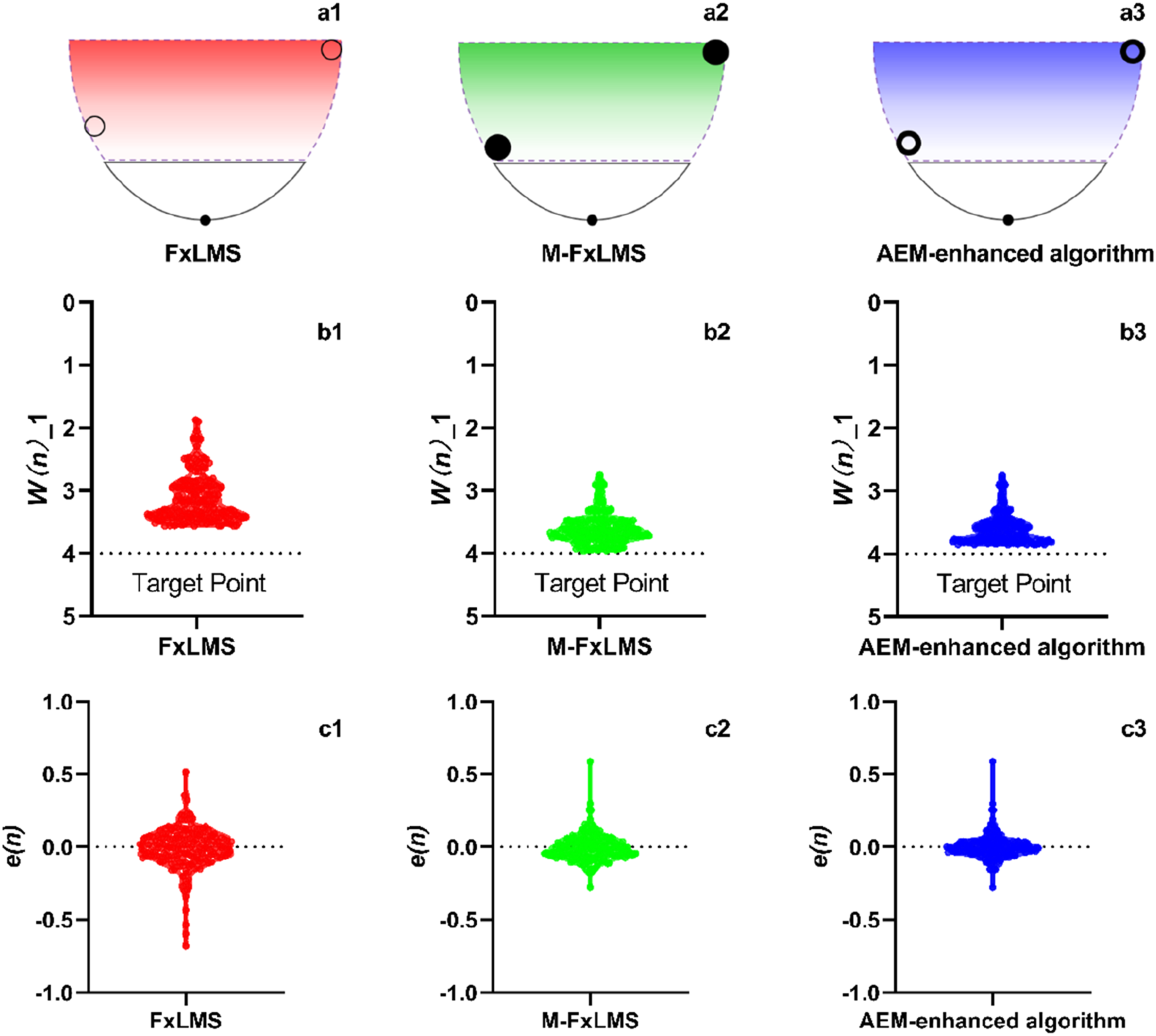
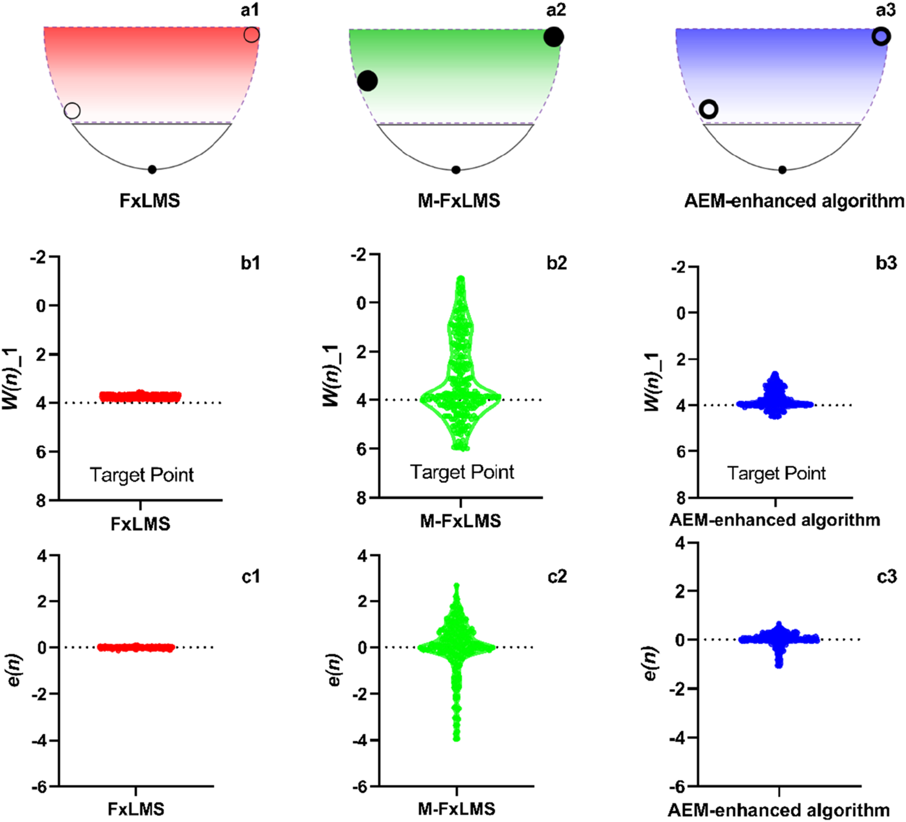
The final stage of iteration process. (a) Different algorithm trace ranges of $W (n)$ (b) Different algorithmic statistical distributions of $W (n)_1$ (c) Different algorithmic statistical distributions of the residual error signal $e (n)$ .

The plot in Figure 4 illustrates that during the initial iteration phase, the M-FxLMS algorithm overall distribution (b2) is notably closer to the target point compared to FxLMS (b1). Moreover, the range of track points in this distribution is significantly narrower than in FxLMS, indicating that M-FxLMS algorithm achieves the optimal weight coefficient at an accelerated rate in the early stages of iteration. This results in a reduction of deviation and oscillation in the optimization process. This leads to a more densely concentrated distribution of iterative residuals (observed in the comparison between c1 and c2). This behavior is elucidated in Section 2.3: the Momentum-FxLMS algorithm can be construed as an FxLMS algorithm with an increased iteration step. This comparison can be likened to a “ball” with greater inertia rolling from the edge of a “bowl” during the optimization iteration process (observed in the comparison between a1 and a2), thereby accelerating the descent in the optimization process. However, owing to the effect of inertia, the M-FxLMS algorithm displays a distribution more akin to a diamond as opposed to the pyramid-like shape observed in the FxLMS algorithm (b1 Vs. b2). Upon comparing b3, b2, b1, it becomes apparent that the AEM-enhanced algorithm amalgamates the merits of the other two algorithms. The trajectory points exhibit a narrow range in close proximity to the optimal weight coefficient, displaying a pyramid-like distribution. This configuration ensures the most rapid convergence speed. The affirmation of this observation lies in the comparison of residual errors. This phenomenon is primarily attributed to the AEM, proposed within this paper. AEM employs a switching coefficient to clip and splice the M-FxLMS and FxLMS algorithms, combining their individual strengths. This conceptualization can be envisioned as the substitution of a “partially inertial ball” (a3) for both the “non-inertial ball” (a1) and the “fully inertial ball” (a2). As a result, during the initial iteration comparisons, the AEM-enhanced algorithm demonstrates the best convergence performance.

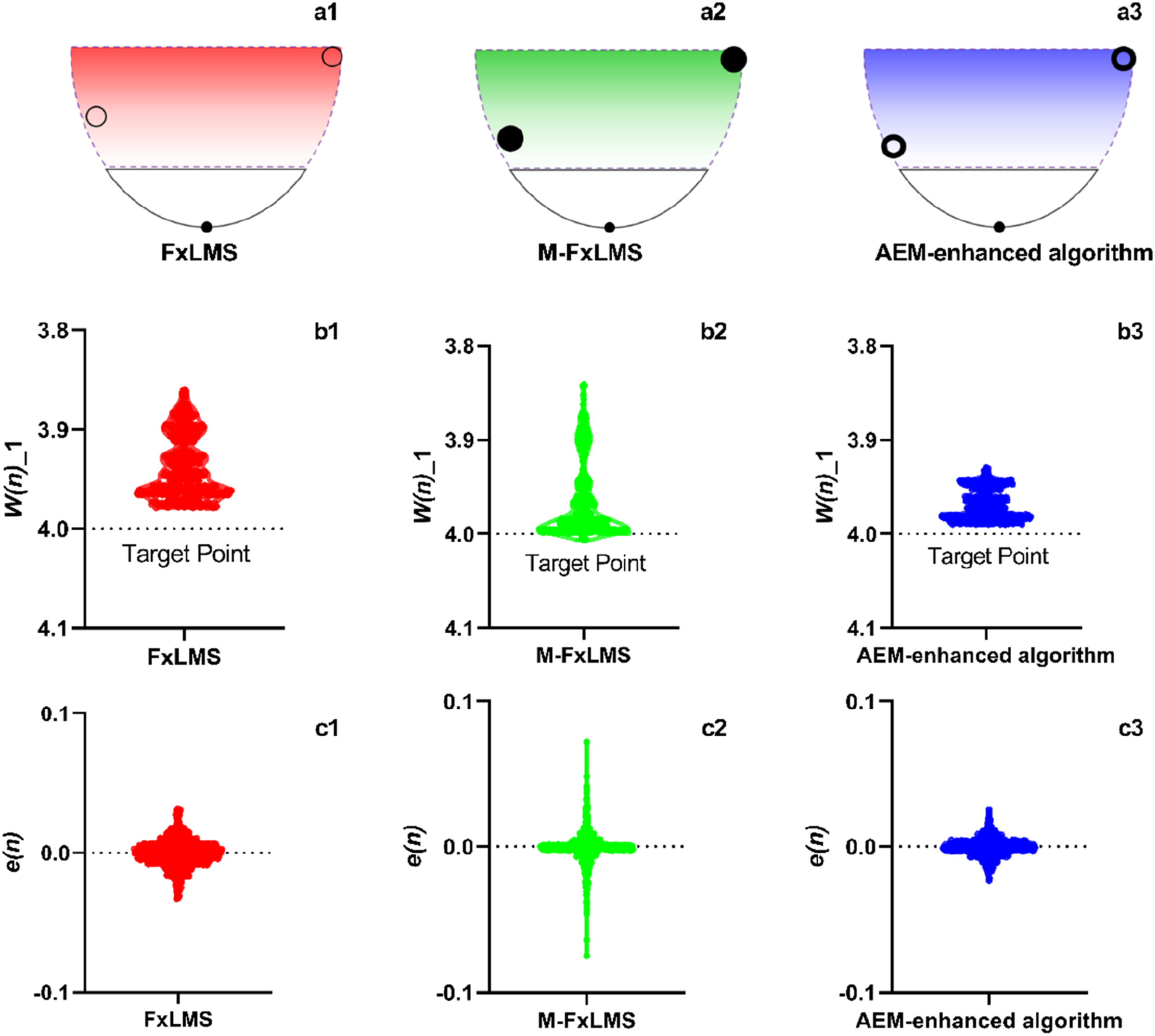
In Figure 5, it is evident that in the middle stage of iteration, notable oscillations were detected in b2 near the optimal weight coefficient. This behavior can be primarily ascribed to the adverse influence of the inertia associated with the M-FxLMS algorithm during the optimization process. As a result, this occurrence induced discernible oscillations in the residual signal (c2), subsequently impacting the convergence speed. In reference to the FxLMS algorithm (illustrated by b1), it is apparent that the absence of inertia results in minimal oscillation during this phase. Additionally, the trajectory points are predominantly clustered in close vicinity to the optimal weight coefficient. In contrast, The AEM-enhanced algorithm (b3) effectively mitigated the adverse effects of inertia. As a result, the oscillation amplitude of its trajectory points demonstrated a notable decrease in comparison to M-FxLMS (b2). Regarding the residual signal, the AEM-enhanced algorithm (c3) displays a noticeable enhancement when compared to M-FxLMS (c2). Nevertheless, its concentration level of the residual signal does not reach the same degree as achieved by FxLMS (c1). Consequently, during the evaluation of the middle stage of iteration, the AEM-enhanced algorithm demonstrates intermediate convergence performance. The M-FxLMS algorithm exhibits the least favorable performance, while the FxLMS algorithm proves the most effective.

In the final stage of the iteration, illustrated in Figure 6, it becomes evident that while M-FxLMS (b2) displays a greater oscillation amplitude in contrast to FxLMS (b1), its track point distribution is predominantly focused around the optimal weight coefficient. Conversely, FxLMS (b1) exhibits a more concentrated track point distribution, albeit positioned farther from the optimal weight coefficient. This disparity results in a broader distribution of iteration errors, as demonstrated by the comparison between c2 and c1. Compared to M-FxLMS (b2), the AEM-enhanced algorithm (b3) exhibits a concentrated distribution of track points with reduced oscillation. In contrast to FxLMS (b1), the track points are notably closer to the optimal weight coefficient. This behavior is primarily attributed to the fact that in the final phase of iteration, the gradient of the loss function experiences a less abrupt change due to the minor variation in residual error. The FxLMS algorithm, lacking consideration for inertia, mistakenly assumes it has attained the optimal point. Nevertheless, as the residual error has not yet met the convergence threshold, the iteration process persists instead of halting, leading to continued iterations around this point. Conversely, when the M-FxLMS algorithm approaches the optimal point, the inertia’s presence induces a gradual oscillation in the iterative trajectory around the optimal point. Nevertheless, its convergence surpasses that of the FxLMS algorithm. The AEM-enhanced algorithm proposed in this paper clip and splices the two algorithms by setting the switching coefficient $ε = 0.01$ . Each switch emulates the inertia adjustment of a ‘ball’. This intervention leads to a diminished oscillation energy within the M-FxLMS algorithm, resulting in a decrease in oscillation amplitude and an improvement in convergence performance. In evaluating the final stage of iteration, it becomes apparent that the AEM-enhanced algorithm demonstrates the most favorable convergence performance, followed by the M-FxLMS algorithm. Conversely, the FxLMS algorithm exhibits comparatively less efficient convergence.

The simulation of robust performance against impulse signals

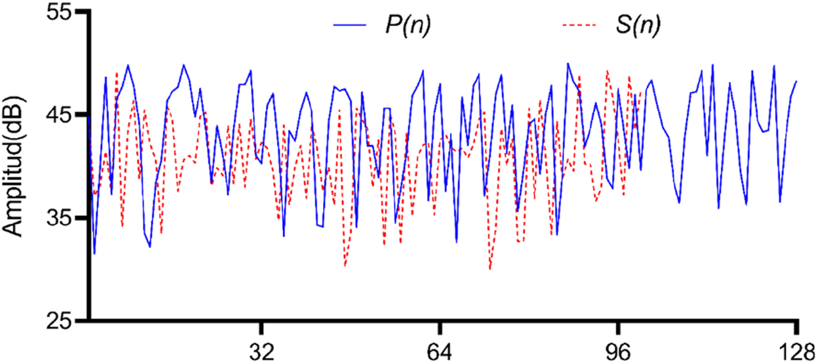
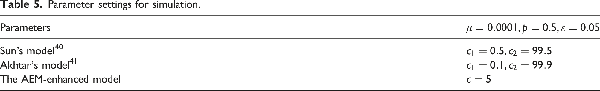
To assess the AEM’s resilience against impulse signals, a 256-order FIR filter for constructing the adaptive filter vector $W (n)$ is utilized. Additionally, a white noise signal with amplitudes ranging from −1 to 1 is employed to form the reference signal $x (n)$ , which comprises a dataset of 50,000 signal points. The primary and secondary path transfer functions, denoted as $P (n)$ and $S (n)$ , respectively, are detailed in Figure 7.

Figure 7.

Primary and secondary path transfer functions.

In two distinct operational cases, involving both reference and system signals, a comparative assessment of impulse robustness across three models is performed: the Sun model,³⁴ the Akhtar model,³⁵ and the AEM-enhanced model outlined in Table 2. The detailed parameter settings are provided in Table 5.

Table 5.

Parameter settings for simulation.

Parameters	$μ = 0.0001, p = 0.5, ε = 0.05$
Sun’s model⁴⁰	$c_{1} = 0.5, c_{2} = 99.5$
Akhtar’s model⁴¹	$c_{1} = 0.1, c_{2} = 99.9$
The AEM-enhanced model	$c = 5$

Case I: Impulse robustness for reference signals

The impulse case is typically marked by an instantaneous large pulse resulting from the impact of the reference signal. In this study, the reference signal

x (n)

incorporates random impulse signals. It is generated by selectively amplifying the signal at ten positions in the white noise, increasing it to ten times its average value. To evaluate the robustness of the three models, the number of iterations necessary for the system to reach stability at the convergence threshold

e < 0.4

of the residual envelope is compared. The outcomes of these simulations are detailed in Table 6, and the iterative procedures for the three models are illustrated in Figure 8.

Table 6.

Simulation results for case I.

Type	Sun’s model	Akhtar’s model	The AEM-enhanced model
Iteration No.	49,999	13,081	12,891

Figure 8.

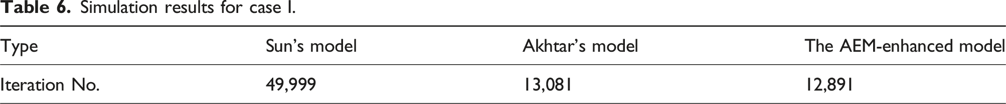
Iteration process of case I. (a) the reference signal (b) the residual error signal.

The findings lead to several key observations. (i) Akhtar’s model demonstrates superior convergence speed when compared to Sun’s model and the AEM-enhanced model exhibits a 74% increase in convergence speed compared to Sun’s model and a 1.5% improvement over Akhtar’s model. (ii) In a stable operational state, both the AEM-enhanced model and Akhtar’s model demonstrate an adeptness in mitigating the impact of impulsive noise within the reference signal. This capability stems from the simultaneous processing of the reference signal $x (n)$ and the residual signal $e (n)$ when impulsive signals emerge. Notably, the AEM-enhanced model presented in this paper employs the algorithm editing method, whereas Akhtar’s model relies on the statistical value replacement method. Sun’s model merely substitutes the impulse signal in the reference signal with a value of 0, without any processing of the residual signal. This leads to a persistent accumulation of calculation errors in the residual signal, ultimately causing significant oscillations until instability arises. (iii) In Sun’s model, the occurrence of multiple consecutive impulses results in larger residual fluctuations when short-term concentrated impulses (Zone 1) are compared to distributed impulses (Zone 2). This phenomenon primarily arises from the system’s limited time for “digesting” the calculation error of the residual signal. The more concentrated the impulse signal distribution, the greater the resultant residual fluctuation. Furthermore, Zone 3 demonstrates that as iterations progress, when these errors accumulate to a certain extent, even a single impulse can induce substantial residual fluctuations. The system’s robustness diminishes with the accumulation of errors. Notably, the AEM-enhanced model, in contrast to Akhtar’s model, does not manifest this issue.

Case II: Impulse robustness for system signals

The incidence of impulses from the system signal surpasses that of the reference signal. This signal perturbation is primarily ascribed to environmental factors, including conversations or sudden coughs within the cabin of a car equipped with an ANC system. These abrupt signals blend with the primary noise and are picked up by the residual microphone. In order to assess the impulse robustness of the three models in this scenario, pulse signals are incorporated to emulate the impact of the system signal. The number of iterations needed for the system to reach stability at the convergence threshold

e < 0.4

of the residual envelope is simulated. The comparative results are presented in Table 7. The iterative processes of the three models are depicted in Figure 9.

Table 7.

Simulation results for case II.

Type	Sun’s model	Akhtar’s model	The AEM-enhanced model
Iteration No.	48,504	38,417	12,906

Figure 9.

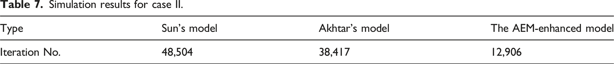
Iteration process of case II. (a) the primary noise signal (b) the residual error signal.

The outcomes lead to several key observations. (i) Both Sun’s and Akhtar’s models display distinct responses to system impact. In contrast, the AEM-enhanced model showcases a 73% and 66% surge in convergence speed, respectively, when compared to Sun’s and Akhtar’s models. This performance enhancement can be primarily attributed to the AEM-enhanced model’s adoption of the algorithm editing method. This method proficiently isolates the impact signal and its associated components, harmonizing the iterative process before and after. Consequently, it ensures steadfast performance in the face of diverse impact scenarios, substantiating its robustness against impacts of varying nature. (ii) In Figure 9(b), it is apparent that Sun’s model exhibits more pronounced oscillations and heightened sensitivity to impact during the stable stage, in contrast to the AEM-enhanced model. The primary reason is its failure to process the residual signal upon impact detection. (iii) When detecting an impact signal, Akhtar’s model simultaneously processes both the impact signal and the residual signal, leading to superior impact resistance performance compared to Sun’s model. Nevertheless, in the later stages of iteration, Akhtar’s model exhibits heightened sensitivity to impulse signals, as illustrated in zones two and three of Figure 9. Both impacts lead the system to exceed the convergence threshold. This concern is non-existent in the AEM-enhanced model. The key reason lies in Akhtar’s model utilizing a global statistical approach to determine the threshold value of the impulse signal. Specifically, in condition non-impulse, the model identifies the signal’s highest peak value, multiplies it by the threshold coefficient, and employs this as an alternative value. To mitigate the impact of the system’s impulse signal, when an impulse is detected, the alternate value is used to replace the actual impulse signal during iteration. Obviously, this method is well-suited for scenarios marked by a generally stable iteration process. However, it may face challenges in instances of significant fluctuation during unstable stages, potentially resulting in an excessively high setting of the alternative value, rendering it less effective in mitigating impulses in stable stages. In contrast, the AEM-enhanced model employs an algorithm editing method to directly eliminate the impulse signal, as opposed to substitution. This approach fosters a consistently stable convergence performance.

Verification test of the algorithm editing method (AEM)

In order to validate the practical application of AEM for improving algorithm performance, a single-input single-output ANC test system is implemented, illustrated in Figure 10. Employed as the control hardware is the dSPACE MicroAutoBox. The system and algorithmic parameters adhere to the specifications provided in Section 3.2.

Figure 10.

The testbench of ANC system.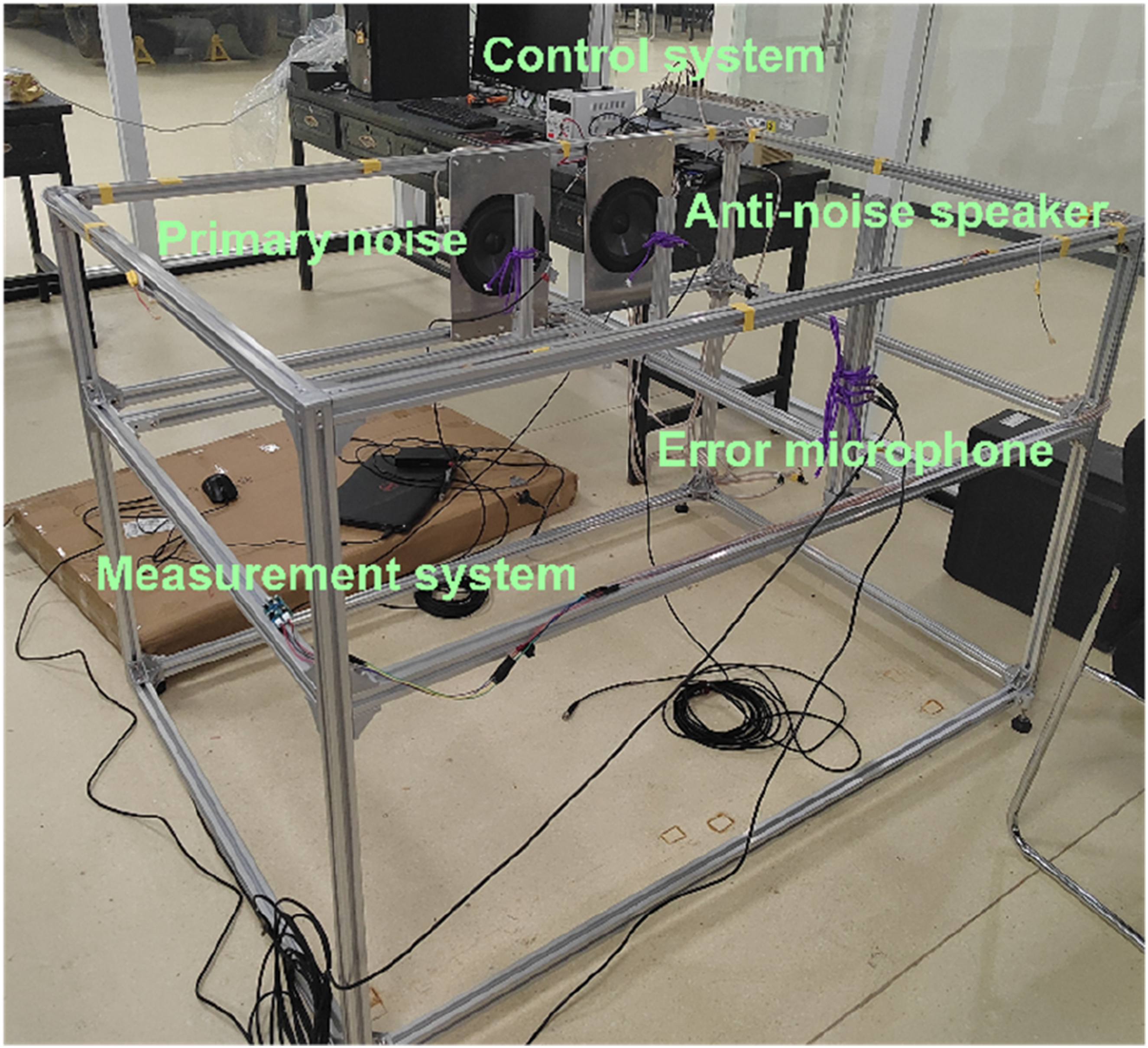

The convergence performance verification

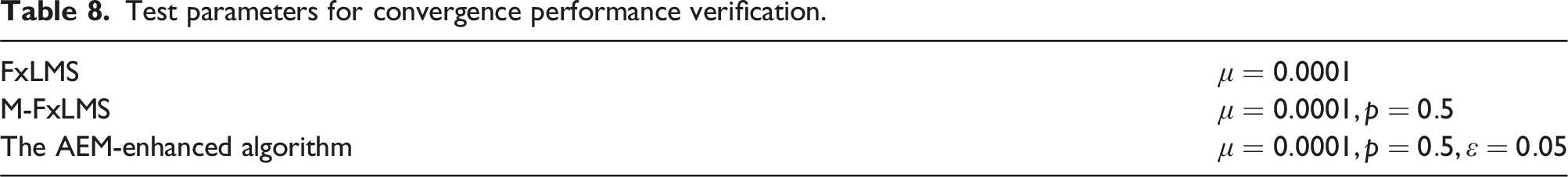
The study provides a comparative analysis of the FxLMS algorithm, the M-FxLMS algorithm, and the proposed AEM-enhanced algorithm. Specific algorithm parameters can be found in Table 8. The sound pressure level was measured with the ANC system activated and deactivated during the test using the LMS Test.Lab test system. The system’s evaluation is based on the overall noise reduction, calculated as the difference of the noises between the ANC system activated and deactivated.

Table 8.

Test parameters for convergence performance verification.

FxLMS	$μ = 0.0001$
M-FxLMS	$μ = 0.0001, p = 0.5$
The AEM-enhanced algorithm	$μ = 0.0001, p = 0.5, ε = 0.05$

The test results are presented in Figure 11. (i) The AEM-enhanced algorithm demonstrates the most effective noise reduction, achieving approximately 12 dB under full convergence. The M-FxLMS algorithm follows with around 10 dB of noise reduction, and the FxLMS algorithm provides about 8 dB of noise reduction. These results align with the findings from the theoretical and simulation analyses above. (ii) In terms of convergence speed, the AEM-enhanced algorithm demonstrates the swiftest stabilization, achieving it in about 1.3 seconds. The M-FxLMS algorithm requires roughly 1.6 seconds to reach stability, while the FxLMS algorithm takes approximately 2.2 seconds, consistent with the earlier analysis.

Figure 11.

Noise attenuation results of various algorithms.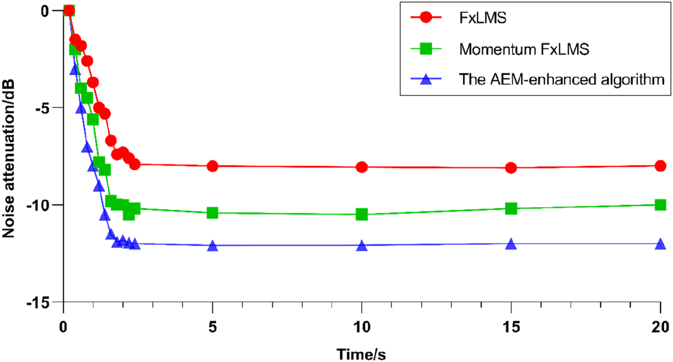

The impulse robustness performance verification

To assess the robustness of AEM against system impulses, eight vigorous claps are generated near the residual microphone in a stable state of operation for the ANC system, simulating a system impulse. The time-domain signal of sound pressure at the controlled position is then recorded during this process for evaluating noise reduction effectiveness.

The test results are presented in Figure 12. (i) The findings indicate that the AEM-enhanced model showcases the most robust resistance to impulses, followed by Akhtar’s model, while Sun’s model displays the least favorable performance. These outcomes are consistent with the conclusions derived from the earlier simulation and theoretical analyses. (ii) In Sun’s model, when subjected to periods of dense impacts (the first five claps), its self-correction capacity diminishes, resulting in reduced noise reduction. This deficiency primarily arises from the model’s inability to rectify the residual signal in response to the impact, leading to the swift accumulation of system errors. Conversely, in instances of sparser impacts (the last three high-fives), there exists sufficient time for error correction, culminating in enhanced noise reduction performance. (iii) The noise reduction performance of Akhtar’s model closely approximates that of the AEM-enhanced model. However, it lacks noise reduction effectiveness for specific impacts, such as the 1st, 2nd, 7th, and 8th claps. This deficiency is especially evident during the 7th and 8th claps, where the loudspeaker emits a distinctive sharp whistling sound. This issue stems from the anti-impact strategy employed in this model, which results in the accumulation of system errors and a tendency towards instability in the later stages of iteration.

Figure 12.

Noise attenuation results for impulse robustness verification.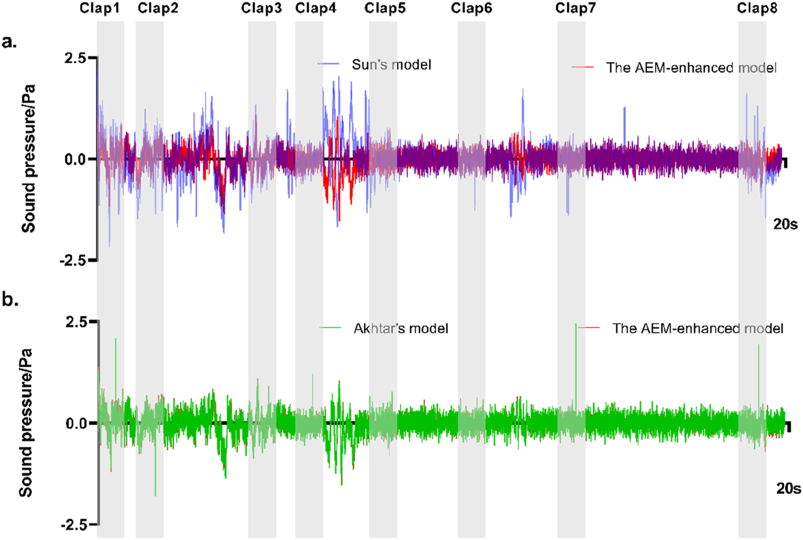

Conclusion

In this study, we propose integrating an Algorithm Editing Method (AEM) into the active noise control system. AEM leverages the distinct characteristics of varied algorithms to enable precise “cutting” and “splicing” of algorithms, tailored to specific iteration stages. The aim is to achieve a balance between convergence rate, stability, and computational efficiency. The effectiveness of AEM is verified using two algorithms: FxLMS and M-FxLMS. The inclusion of the switching coefficient as a trigger condition enables algorithmic splicing and editing that is customized to various iteration stages. Results indicate that, with identical convergence criteria, the AEM-enhanced algorithm accomplishes a considerably faster convergence. When compared to the FxLMS and M-FxLMS algorithms, this algorithm shows respective improvements in convergence speed of 26.7% and 12.8%, without any additional computational complexity. Additionally, the Algorithm Editing Method (AEM) is utilized in this study to enhance the anti-impulse capabilities of the algorithms. The study shows that the AEM-enhanced model exhibits better impulse robustness when compared to Sun’s and Akhtar’s models. Additionally, it has a significant advantage in limiting the impact of system signals.

Footnotes

Declaration of conflicting interests

The author(s) declared no potential conflicts of interest with respect to the research, authorship, and/or publication of this article.

Funding

The author(s) disclosed receipt of the following financial support for the research, authorship, and/or publication of this article: This research was partially supported by Henan Provincial Science and Technology Tackling Project (No.242102241054). It is also supported by Scientific Research Start-up Fund for High-level Talents of Henan Institute of Technology (No.XJ2023000903)

ORCID iD

Zhiyong Chen

References

Kim

Altinsoy

. An experimental investigation of active control of road noise employing the weighted error signal to maximize the noise suppression performance at focused control positions. Appl Acoust 2023; 209: 109408.

Shi

Lam

Shen

, et al. Multichannel two-gradient direction filtered reference least mean square algorithm for output-constrained multichannel active noise control. Signal Process 2023; 207: 108938.

Mostafavi

Cha

. Deep learning-based active noise control on construction sites. Autom ConStruct 2023; 151: 104885.

Pradhan

Zhang

Zhao

, et al. On eigenvalue shaping for two-channel decentralized active noise control systems. Appl Acoust 2023; 205: 109260.

Cha

Mostafavi

Benipal

. DNoiseNet: deep learning-based feedback active noise control in various noisy environments. Eng Appl Artif Intell 2023; 121: 105971.

Chu

Mak

, et al. A new variable spatial regularized FxLMS algorithm for diffusion active noise control. Appl Acoust 2023; 211: 109532.

Mazur

Wrona

Chraponska

, et al. FxLMS with multiple error switching for active noise-cancelling casings. Arch Acoust Q 2019; 44(4): 775–782.

Ferrer

García-Mollá

Vidal-Maciá

, et al. Assessment of stability of distributed FxLMS active noise control systems. Signal Process 2023; 210: 109087.

Gong

Guo

, et al. Statistical analysis of multichannel FxLMS algorithm for narrowband active noise control. Signal Process 2022; 200: 108646.

10.

Wang

Guo

, et al. Active control for vehicle interior noise based on DWT-FxLMS algorithm using a piezoelectric feedback system. Appl Acoust 2020; 167: 107409.

11.

Chen

Yang

. A distributed FxLMS algorithm for narrowband active noise control and its convergence analysis. J Sound Vib 2022; 532: 116986.

12.

Tobias

Bermudez

JCM

Bershad

. Mean weight behavior of the filtered-x LMS algorithm. IEEE Trans Signal Process 2000; 48: 1061–1075.

13.

Vicente

Masgrau

. Novel FxLMS convergence condition with deterministic reference. IEEE Trans Signal Process 2006; 54: 3768–3774.

14.

Hermont

IKde S

Flores

de Lamare

. Robust adaptive filtering based on the hyperbolic tangent exponential Kernel M-estimator function for active noise cancellation. In: 2024 19th International Symposium on Wireless Communication Systems (ISWCS). Rio de Janeiro, Brazil, 14-17 July 2024, 2024, pp. 1–6. DOI: 10.1109/ISWCS61526.2024.10639117.

15.

Aslam

Shi

Lim

. Robust active noise control design by optimal weighted least squares approach. IEEE Trans Circ Syst I 2019; 66(10): 3955–3967.

16.

Zhou

Xia

, et al. An efficient algorithm for impulsive active noise control using maximum correntropy with conjugate gradient. Appl Acoust 2022; 188: 108511.

17.

Qiu

Burnett

, et al. A recursive least square algorithm for active control of mixed noise. J Sound Vib 2015; 339: 1–10.

18.

Zhu

Yang

, et al. Conjugate gradient-based FLANN algorithms in nonlinear active noise control. J Franklin Inst 2022; 359(9): 4468–4488.

19.

Zhou

Zhao

Liu

, et al. Combined step size affine-projection-like exponential hyperbolic sine algorithm for robust active noise control. Mech Syst Signal Process 2024; 221: 111716.

20.

Wang

Xiao

, et al. A new hybrid active noise control system with input-power-controlled online secondary-path modeling. IEEE/ACM Trans Audio Speech Lang Process 2024; 32: 3157–3170.

21.

Vazquez

Garcia

Avalos

, et al. A high-precision multi-arithmetic neural circuit for the efficient computation of the new filtered-X Kronecker product APL-NLMS algorithm applied to active noise control. Expert Syst Appl 2022; 191: 116255.

22.

Park

Kim

Gwak

, et al. Active noise control algorithm robust to noisy inputs and measurement impulsive noises. In: 20th International Conference on Control, Automation and Systems (ICCAS), Busan, Korea, 13-16 October 2020, 2020: 622–626.

23.

Kim

Lee

, et al. Novel active noise control based on a robust filtered-x normalized least mean square sign algorithm against large measurement and impulsive noises. In: 20th International Conference on Control, Automation and Systems (ICCAS), Busan, Korea, 13-16 October 2020, 2020, pp. 617–621.

24.

Xiao

, et al. Statistical analysis of narrowband active noise control using a simplified variable step-size FxLMS algorithm. Signal Process 2021; 183: 108012.

25.

Meng

Chen

. Particle swarm optimization based novel adaptive step-size FxLMS algorithm with reference signal smoothing processor for feedforward active noise control systems. Appl Acoust 2021; 174: 107796.

26.

Puri

Modak

Gupta

. Global active control of harmonic noise in a vibro-acoustic cavity using Modal FxLMS algorithm. Appl Acoust 2019; 150: 147–161.

27.

Gomathi

Saravanan

Santhiya kumari

. Variable step size for improving convergence of FxLMS algorithm. Procedia Technology 2016; 25: 420–426.

28.

Shynk

Roy

, The LMS algorithm with momentum updating. In: IEEE International Symposium on Circuits and Systems.Espoo, Finland, 07-09 June 1988, 1988, Vol. 3, pp. 2651-2654.

29.

Sun

, et al. A variable momentum factor filtered-x weighted accumulated LMS algorithm for narrowband active noise control systems. Measurement 2014; 48: 282–291.

30.

Padhi

Chandra

Kar

, et al. A new adaptive control strategy for hybrid narrowband active noise control systems in a multi-noise environment. Appl Acoust 2019; 146: 355–367.

31.

Cheng

Chen

, et al. Active control of impulsive noise based on a modified convex combination algorithm. Appl Acoust 2022; 186: 108438.

32.

Zhao

Zeng

, et al. Improved functional link artificial neural network via convex combination for nonlinear active noise control. Appl Soft Comput 2016; 42: 351–359.

33.

Vanamadi

Kar

. Power transfer function based feedback cancellation using convex combination of adaptive filters. In: 19th International Conference on Electrical Engineering/Electronics, computer, Telecommunications and Information Technology (ECTI-CON), Prachuap Khiri Khan, Thailand, 24-27 May 2022, 2022, pp. 1–4.

34.

Kuo

Morgan

. Active noise control systems algorithms and DSP Implementations. New York: Wiley, 1996.

35.

Kuo

Morgan

. Active noise control a tutorial review. Proc IEEE 1999; 87(6): 943–975.

36.

Roy

Shynk

. Analysis of the momentum LMS algorithm. IEEE Trans Acoust Speech Signal Process 1990; 38(12): 2088–2098.

37.

Chien

Tsao

. Affine-Projection-like maximum correntropy criteria algorithm for robust active noise control. IEEE/ACM Trans Audio Speech Lang Process 2022; 30: 2255–2266.

38.

Kranthi

Vasundhara . A robust adaptive filter for diffusion strategy-based distributed active noise control. IETE J Res 2023; 70(5): 5066–5080.

39.

Turpati

Roy

Swamy

KCT

, et al. Robust non-Linear active function-based FxRLS for impulsive active noise control. IEEE Access 2024; 12: 43222–43234.

40.

Sun

Kuo

Meng

. Adaptive algorithm for active control of impulsive noise. J Sound Vib 2006; 291(1-2): 516–522.

41.

Tahir Akhtar

Mitsuhashi

. Improving performance of FxLMS algorithm for active noise control of impulsive noise. J Sound Vib 2009; 327: 647–656.

Research and application of the algorithm editing method for improving active noise control performance

Abstract

Keywords

Introduction

Development of the algorithm editing method (AEM)

Description of ANC system

The filtered-x least mean square (FxLMS) algorithm

The momentum FxLMS (M-FxLMS) algorithm

The algorithm editing method (AEM)

A study of the rate of convergence of algorithms

A study of the misalignment of algorithms

The advantages of the algorithm editing method (AEM)

Applications of the algorithm editing method

Simulation of the performance of the algorithm editing method (AEM)

The convergence performance simulation

The simulation of robust performance against impulse signals

Case I: Impulse robustness for reference signals

Case II: Impulse robustness for system signals

Verification test of the algorithm editing method (AEM)

The convergence performance verification

The impulse robustness performance verification

Conclusion

Footnotes

Declaration of conflicting interests

Funding

ORCID iD

References