Resonance analysis based on the Galerkin technique and coupled nonlinear Mathieu equations that have been renormalized

Abstract

The stability evaluation of damping-coupled Mathieu-type equations necessitates robust analytical methodologies. To conquer the limitations of small-parameter assumptions inherent in perturbative strategies, the non-autonomous system is transformed into an equivalent autonomous system, simplifying the analysis. The Galerkin technique provides a powerful foundation for investigating these complex systems by carefully including oscillator coupling to capture problematic electricity transfer and interaction consequences that are frequently overlooked in traditional approaches. The coupled Galerkin approach enables a comprehensive study of balance behavior, offering significant insights into the effects of oscillator coupling on typical balance. The method highlights the effects of coupling on resonance stability transitions, such as internal and harmonic resonances, by determining stability barriers via essential parameter evaluation. This method provides a radical insight into the stability dynamics of coupled Mathieu oscillators. It is a critical tool for engineering and science applications that require precise control over complicated oscillatory systems.

Introduction

A wide range of real-world phenomena from several fields, including plasma physics, fluid dynamics, optics, quantum mechanics, cosmology, biology, and chemistry, were effectively represented using differential equations. These equations have also been useful in addressing complicated engineering challenges and other complex systems. ¹ The Mathieu equation, a fundamental model of parametrically excited systems, has been extensively researched for its balancing and resonance behaviors.^2,3 The Mathieu equation stands out as a particularly broad differential equation due to its large-scale applications in a variety of industries. Its significance has piqued academics’ interest, particularly in defining systems with periodic coefficients. In quantum systems involving capacity power, the Mathieu equation is undoubtedly derived from the Schrödinger equation. In these cases, the quantum gadget’s wave functions correspond to the periodic eigenfunctions of the Mathieu equation. This relationship emphasizes the equation’s application in quantum physics, particularly when quantum devices encounter cosine-like capacity power fields.^4,5 Its programs expand further to scenarios governed by periodic ability implications, establishing the Mathieu equation as an essential tool for reading complex quantum behaviors. Despite the utility and relative simplicity of numerically solving linked Mathieu equations under specified conditions, a preferred analytic solution has yet to be established. This problem emphasizes the inherent difficulties in accurately photographing the dynamics of such formations. Nonetheless, numerical methodologies provide definite and understandable answers, supporting the equation’s applicability across a wide range of scientific and practical applications.

The coupled Mathieu oscillator is a dynamic system defined by coupled differential equations with parametric excitation. Such structures play an important role in representing a wide range of physical phenomena, including vibrations in mechanical structures, stability in engineering systems, and quantum mechanical behaviors. Parametric resonances and associated restriction cycles occur at both the main and aggregate resonance frequencies in multi-coupled systems. ⁶ The existence of cubic nonlinearities also complicates the device’s reactivity, resulting in complex stability and bifurcation scenarios.^7–9 The well-known observation of parametric resonance in conservative coupled oscillator systems demonstrates that eigenmodes can cause parametric amplification, also known as auto-parametric resonance. This phenomenon includes energy switching between modes, which significantly influences the system’s dynamic responsiveness. ¹⁰ Recent research has focused on the resonance simulation of coupled nonlinear Mathieu equations, highlighting their applications in domains such as plasma physics, optics, and quantum mechanics. These studies stress the need to understand the stability and resonance behavior of such systems for practical applications.^11,12 The coupled Mathieu oscillator is a key variant for investigating the complex dynamics of coupled objects under parametric activation. Its evaluation provides critical insights into the stability, resonance phenomena, and power switch mechanisms seen in complex oscillatory systems. It applies to electromechanical systems, including micro-electromechanical structures (MEMS), where nonlinear interactions and coupling effects are critical.^13,14 Furthermore, the oscillator is useful in fluid-shape interaction studies, electricity harvesting technologies, and structure characterization using multi-scale coupling dynamics. This adaptability makes it an effective tool for investigating and comprehending a wide range of real-world events.^15,16

The stability of coupled Mathieu oscillators, driven by coupled differential equations that incorporate damping and parametric excitation, is a key task in the study of dynamic structures. ¹⁰ Inner and harmonic resonance responses are important phenomena in such devices because they occur when the frequency of an external stimulation or internal coupling matches or interacts with the device’s inherent frequencies.

Parametric resonance is an exceptional phenomenon that occurs when the excitation frequency coincides with one of the system’s inherent frequencies, resulting in enhanced oscillations. These enhanced responses can have a significant impact on the stability and function of the device, making parametric resonance an important concern in structures exposed to periodic external stresses, such as vibrating systems, spinning equipment, and auditory structures. ¹⁷ Internal resonance in assessment refers to the interplay of various herbal frequencies within a device, which is typically caused by nonlinear coupling between modes. This interaction causes power exchange between modes, which manifests as complex oscillatory behaviors, amplitude modulations, or possibly chaotic dynamics.^18,19 These troublesome occurrences frequently affect machine behavior, but they also present great opportunities for energy switching and optimization in positive applications.

Internal and harmonic resonance responses play an important role in engineering applications such as structural stability design, vibration manipulation in mechanical structures, optimization of electricity harvesting devices, and mitigation of resonance-induced errors in aerospace, automotive, and civil engineering domains. A thorough understanding of these responses is required for accurately anticipating and managing dynamic behavior, assuring the stability and overall performance of real-world systems.^1,20

El-Dib’s frequency formula is a highly effective analytical tool for investigating nonlinear and parametric oscillators. It systematically determines the effective natural frequencies of complex systems by accounting for key factors such as damping and external forces. Unlike traditional methods, El-Dib’s formula incorporates the combined effects of parametric excitation and coupling, making it particularly adept at analyzing systems like Mathieu oscillators.^21–23 A notable feature of this formula is its ability to transform non-autonomous systems into equivalent autonomous systems. This transformation simplifies the analysis, allowing for the estimation of approximate but highly accurate frequencies under the framework of the Harmonic Equivalent Linearization Method (HELM). Such precision is essential for understanding the complete dynamic behavior of systems undergoing resonance or instability.^24–26

By enabling the conversion to an autonomous form, El-Dib’s formula provides a robust foundation for stability analysis, identification of critical parameters, and the design of dynamic systems. Its practical applications span a wide range of fields, including structural engineering, mechanical systems, and vibrational analysis, where precise control over oscillatory behavior is vital.^27,28 Its versatility extends to a wide range of applications, including mechanical and structural engineering, fluid-structure interactions, and vibrational analysis. These domains require precise control over oscillatory behaviors, making El-Dib’s frequency formula an indispensable tool for understanding and managing dynamic systems effectively.

Kwasniok ²⁹ describes a technique for creating fundamental ODE structures that simulate the dynamics of nonlinear PDEs. The authors extract function spatial structures, or important interaction styles, using a nonlinear variational approach based on a dynamical optimality criterion. These patterns are then employed as foundation functions in a Galerkin approximation, significantly reducing the complexity of the original PDE device.^30,31 The Galerkin technique is an important analytical tool in engineering, especially for studying resonance phenomena in structures such as vibrating beams, plates, and linked oscillators. This method reduces complex partial differential equations to a finite collection of ordinary differential equations by projecting governing equations onto a set of basis functions that reproduce the machine’s natural vibration patterns. This reduction allows for a better understanding of transitions to instability caused by nonlinear findings or parametric forcing, which is crucial for maintaining balance beneath resonance—a critical design consideration.^32–34 The Galerkin technique is an effective tool for understanding balance and resonance phenomena in dynamic systems.^22,35 The Galerkin approach reduces complex partial differential equations to a limited collection of ordinary differential equations by projecting the governing equations onto a defined set of basic functions, which are typically chosen to mimic the machine’s fundamental modes of vibration. ³⁶ This reduction is particularly useful for interpreting resonance since it captures the dominant dynamic pattern while reducing mathematical complexity. In the context of balancing, the method provides a scientific approach to examining how external periodic excitations interact with the system’s intrinsic frequencies, potentially leading to resonance. By focusing on resonance circumstances, the Galerkin technique allows for the discovery of critical characteristics such as damping, stiffness, and excitation amplitude that affect balance.^22,35

The proposed study investigates the stability and dynamic behavior of coupled-damped oscillatory systems driven by Mathieu equations, employing sophisticated analytical techniques such as the re-normalized approach and the Galerkin approach. The study investigates the complexities of systems that use parametric forcing, interaction effects, and matched oscillations. This work evaluates balancing constraints, resonance phenomena, and electricity transmission methods, providing useful insights applicable to engineering domains such as vibrating structures, fluid-shape interactions, and electromechanical structures. The findings aim to improve the design and performance of such systems, especially in situations where correctly dealing with nonlinear behaviors is crucial to balance and capacity.

A brief explanation of the renormalization approach (RA)

The renormalization approach is an analytical strategy that uses the least squares method and weighted averaging to deal with parametric linear or nonlinear oscillations under periodic forcing, rather than relying on physical assumptions or small-amplitude approximations. Even for large stimulation amplitudes, this approach performs well in terms of numerical results. It provides a unique framework for converting non-autonomous structures into equivalent self-reliant papers, simplifying the response process and allowing for effective balance evaluation.

To exemplify the renormalization technique for changing a non-autonomous system into an autonomous form, consider the following second-order differential equation with periodic Hill coefficients:

$\ddot{u}+\psi \left(t\right)u=0,$

(1)

where $\psi \left(t\right)$ is a periodic function with variable t. To convert equation (1) to an autonomous form, an alternate systematic transformation is required. The elimination of explicit time dependence while maintaining the basic dynamics of the system is a critical prerequisite. The proposed alternative form is that.

$\ddot{u}+{\varpi }^{2}u=0.$

(2)

This approximates the true equation (1). When comparing equations (2) and (1), several mistakes arise. The least squares approach can be used to calculate an unknown constant, ${\varpi }^2$ . This strategy uses a weighted function. To estimate the error E( $\varpi$ ), multiply both sides of equations (1) and (2) by a weighted function $\chi \left(t\right)$ , as follows:

$E\left(\varpi \right)=\left|\left(\psi \left(t\right)-{\varpi }^2\right)\chi \left(t\right)\right|.$

(3)

Weighted average functions are useful in a variety of applications, including approximation, computational efficiency, and data analysis. They are extremely useful in the least square’s method, which enhances model precision and reliability. The mean square error is a widely used metric for calculating the average squared difference between estimated and actual data. The definition is as follows:

${\overline{E}}^2\left(\varpi \right)=\underset{0}{\overset{2\pi }{{\displaystyle \int }}}{\left(\psi \left(t\right)-{\varpi }^2\right)}^2{\chi }^2\left(t\right)dt.$

(4)

where T is the period. The error’s minimum value requires that

$\frac{d{\overline{E}}^2}{d{\varpi }^2}=\frac{d}{d{\varpi }^2}\underset{0}{\overset{2\pi }{{\displaystyle \int }}}\left({\psi }^2\left(t\right)-2{\varpi }^2\psi \left(t\right)+{\varpi }^4\right){\chi }^2\left(t\right)dt=0.$

(5)

The function $\psi \left(t\right)$ remains unaffected by differentiation around the parameter ${\varpi }^2,$ as it is independent of it. Consequently,

$\frac{d{\overline{E}}^2}{d{\varpi }^2}=2\underset{0}{\overset{2\pi }{{\displaystyle \int }}}\left({\varpi }^2-\psi \left(t\right)\right){\chi }^2\left(t\right)dt=0.$

(6)

Solving the preceding equation for ${\varpi }^2$ yields

${\varpi }^2=\frac{\underset{0}{\overset{2\pi }{{\displaystyle \int }}}\psi \left(t\right){\chi }^2\left(t\right)dt}{\underset{0}{\overset{2\pi }{{\displaystyle \int }}}{\chi }^2\left(t\right)dt}.$

(7)

Assume the perturbed natural frequency $\psi \left(t\right)$ and the suitable weighted function $\chi \left(t\right)$ are supplied, respectively, as:

$\psi \left(t\right)=a+q\hspace{0.17em}{\mathit{cos}}^2\hspace{0.17em}\omega t,\text{and}\hspace{0.17em}\chi \left(t\right)=\mathit{cos}\hspace{0.17em}nt;n=1,2,3,...$

(8)

This assumption allows equation (1) to be the well-known Mathieu equation with total frequency ${\varpi }^2$ . In terms of assumption (8), the constant frequency ${\varpi }^2$ can be estimated as follows:

${\varpi }_n^2=a+q\left(\frac{1}{2}+\frac{\left(2{\omega }^2-n^2\right)\mathit{sin}\left(4\pi \omega \right)}{8\pi \omega \left({\omega }^2-n^2\right)}\right).$

(9)

Thus, the approximate solution to the Mathieu problem can be expressed as

$u\left(t\right)=A_n\hspace{0.17em}\mathit{cos}\hspace{0.17em}{\varpi }_{n}t+B_n\hspace{0.17em}\mathit{sin}\hspace{0.17em}{\varpi }_{n}t,$

(10)

where A_n and B_n represent arbitrary constants. In contrast to relying on several perturbed issues and modest parameters, converting the non-autonomous oscillator into an autonomous version offers significant advantages. These results are consistent with those obtained by traditional perturbation approaches. This change offers a more modern and robust paradigm that allows nonlinear structures to be evaluated without being constrained by the weak nonlinearity assumption. It is highlighted that the case ${\omega }^2\cong n^2$ acts as a resonance point.22

Significance of the problem

The two-coupled parametric system with damping integrates intricate interactions between two oscillators, encompassing damping effects, linear coupling, and parametric excitation. A detailed understanding of the role played by each parameter enables a thorough analysis of the system’s dynamic behavior. This analysis provides critical insights into stability conditions, resonance phenomena, and energy transfer mechanisms, which are essential for exploring the system’s potential applications in engineering and physics. The damping parametric system can be expressed as follows:

$\ddot{x}+{\mu }_{11}\dot{x}+{\mu }_{21}\dot{y}+\left(a_{11}+q_{11}\hspace{0.17em}{\mathit{cos}}^2\hspace{0.17em}\omega t\right)x+p_{11}{x}^3+\left(a_{21}+q_{21}\hspace{0.17em}{\mathit{cos}}^2\hspace{0.17em}\omega t\right)y+p_{21}{y}^3=0,$

(11)

$\ddot{y}+{\mu }_{22}\dot{y}+{\mu }_{12}\dot{x}+\left(a_{22}+q_{22}\hspace{0.17em}{\mathit{cos}}^2\hspace{0.17em}\omega t\right)y+p_{22}{y}^3+\left(a_{12}+q_{12}\hspace{0.17em}{\mathit{cos}}^2\hspace{0.17em}\omega t\right)x+p_{12}{x}^3=0.$

(12)

In this model, x(t)​ and y(t) represent the displacement variables of the coupled systems, ω denotes the excitation frequency, ${\mu }_{ij}$ is the damping coefficient, $a_{ij}$ represents the constant natural frequency, $p_{ij}$ refers to the Duffing’s coefficient, and ${\hspace{0.17em}q}_{ij}$ corresponds to the amplitude of the perturbed natural frequency. This versatile formulation can simulate a wide array of physical systems, such as vibrating mechanical structures, coupled oscillators, and vibrational fluids. ¹⁶ It is particularly effective for modeling the motion of beams or plates under periodic external loads. The system exhibits linear vibrations driven by parametric stimulations.

The initial conditions for the system are typically assumed as:

$x\left(0\right)=A,\dot{x}\left(0\right)=0\text{and}y\left(0\right)=B,\dot{y}\left(0\right)=0.$

(13)

The initial conditions in differential equations identify arbitrary constants of integration, ensuring uniqueness, and relevance. They assume a known physical state, providing boundary information for dynamic system analysis and describing coupled oscillators’ time-dependent behavior.

The system described by equations (1) and (2) represent two-coupled harmonic oscillators with variable coefficients, exhibiting damping and Mathieu-type characteristics. The presence of perturbations in the natural frequencies introduces a non-autonomous configuration to the system. However, by approximating these perturbed natural frequencies with an estimated constant frequency, the system can be transformed into an autonomous form. El-Dib’s formula provides a systematic method for incorporating the effects of damping, parametric excitation, and coupling into the approximation of natural frequencies. By substituting these approximated frequencies into the system’s governing equations, the equations are reformulated into an autonomous form, simplifying the study of stability, resonance, and dynamic responses. This transformation allows the equations to be reformulated as:

$\ddot{x}+{\mu }_{11}\dot{x}+{\varpi }_{11}^2\left(\omega \right)x+p_{11}{x}^3+{\mu }_{21}\dot{y}+{\varpi }_{21}^2\left(\omega \right)y+p_{21}{y}^3=0,$

(14)

$\ddot{y}+{\mu }_{22}\dot{y}+{\varpi }_{22}^2\left(\omega \right)y+p_{22}{y}^3+{\mu }_{12}\dot{x}+{\varpi }_{12}^2\left(\omega \right)x+p_{12}{x}^3=0.$

(15)

This reformulated autonomous representation provides a more straightforward framework for analyzing the stability and dynamic behavior of the coupled system, where there ${\varpi }_{ij}^2\left(\omega \right);i,j=1,2$ are modified natural frequencies of the two oscillators (4) and (5). The system’s non-autonomous nature can be simplified by transforming it into an equivalent autonomous form, facilitating the analysis of its stability and dynamic behavior. This transformation relies on approximating the perturbed natural frequencies using El-Dib’s frequency formula,^21,22,26 which is expressed as:

${\varpi }_{ij}^2\left(\omega \right)=\frac{\underset{0}{\overset{2\pi }{{\displaystyle \int }}}{\mathit{cos}}^2\hspace{0.17em}t\left(a_{ij}+q_{ij}\hspace{0.17em}{\mathit{cos}}^2\hspace{0.17em}\omega t\right)dt}{\underset{0}{\overset{2\pi }{{\displaystyle \int }}}\left({\mathit{cos}}^2\hspace{0.17em}t\right)dt}=a_{ij}+\frac{1}{2}{q}_{ij}\left(1+\frac{\left(2{\omega }^2-1\right)\mathit{sin}\left(4\pi \omega \right)}{4\pi \omega \left({\omega }^2-1\right)}\right);i,j=1,2$

(16)

These autonomous equations (14) and (15) simplify the analysis of the system’s dynamics by removing the complication associated with variable coefficients. This reformulation facilitates the examination of the system’s stability, resonance, and coupled nonlinear behavior. The linear equivalent theory can be used to turn the system’s nonlinear oscillation into its linear equivalent. This requires determining the system’s equivalent frequency. Using El-Dib’s^24–26 procedures, we obtain linear damping-coupled equations. Knowing these characteristics allows for an accurate description of the system’s damping behavior, resulting in a more straightforward solution.

$\ddot{x}+{\mu }_{11}\dot{x}+{\sigma }_{11}^{2}x+{\mu }_{21}\dot{y}+{\sigma }_{21}^{2}y=0,$

(17)

$\ddot{y}+{\mu }_{22}\dot{y}+{\sigma }_{22}^{2}y+{\mu }_{12}\dot{x}+{\sigma }_{12}^{2}x=0,$

(18)

where the modified natural frequencies ${\sigma }_{ij}^2\left(\omega \right)$ can be estimated under the assumption of the trial solutions that are assumed in the form

$x_0\left(t\right)=A\hspace{0.17em}\mathit{cos}\hspace{0.17em}{\Omega }_{1}t\hspace{0.17em}\text{and}{\hspace{0.17em}y}_0\left(t\right)=B\hspace{0.17em}\mathit{cos}\hspace{0.17em}{\Omega }_{2}t.$

(19)

Consequently, we have

${\sigma }_{11}^2={\varpi }_{11}^2\left(\omega \right)+\frac{3}{4}{p}_{11}{A}^2,$

(20)

${\sigma }_{21}^2={\varpi }_{21}^2\left(\omega \right)+\frac{3}{4}{p}_{21}{B}^2,$

(21)

${\sigma }_{12}^2={\varpi }_{12}^2\left(\omega \right)+\frac{3}{4}{p}_{12}{A}^2,$

(22)

${\sigma }_{22}^2={\varpi }_{22}^2\left(\omega \right)+\frac{3}{4}{p}_{22}{B}^2,$

(23)

where A and B denote the amplitudes of the oscillations, whereas ${\Omega }_1$ and ${\Omega }_2$ are the total frequencies, respectively, to be estimated depending on the modified natural frequencies ${\sigma }_{ij}^2$ , as well as the damping coefficients ${\mu }_{ij}.$

To validate the strategy for converting a non-autonomous system into an autonomous one, as well as the transformation to the equivalent linearization approach, a numerical comparison provides valuable confirmation and enhances confidence in the method. Accordingly, Figure 1 presents a numerical comparison between the original non-autonomous system, defined by equations (1) and (2), and the corresponding autonomous system, described by equations (17) and (18), evaluated under the initial conditions outlined in equation (13). This comparison utilizes the specified numerical parameter values to assess how effectively the autonomous transformation approximates the dynamics of the original system. The results aim to illustrate the equivalence and effectiveness of the autonomous representation in capturing the key behaviors of the non-autonomous system.

• Initial amplitudes: $A=1,B=0.5,$

• Damping coefficients: ${\mu }_{11}={\mu }_{22}=0.2,{\mu }_{21}={\mu }_{12}=0.1,$

• Natural frequencies: $a_{11}=2,a_{22}=3,a_{21}=a_{12}=1,$

• Duffing coefficients: $p_{11}=p_{21}=p_{22}=p_{12}=0.01,$

• Parametric excitation amplitude: $q_{11}=q_{21}=q_{22}=q_{12}=1,$

• Parametric excitation frequency: $\omega =10.$

Figure 1.

A numerical comparison of the original 2DOF system with parametric coefficients and the autonomously transformed system.

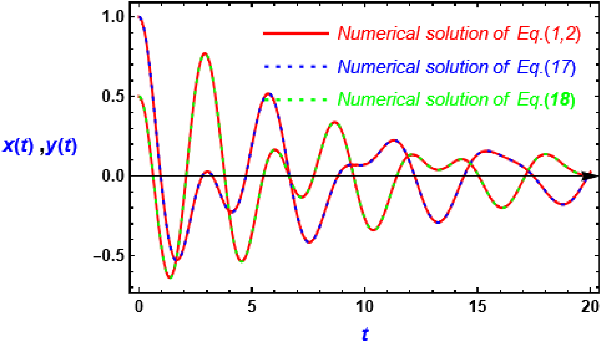
These numbers were chosen to allow for a realistic comparison between non-autonomous and autonomous systems, highlighting their stability and dynamic behavior under similar initial conditions.

Figure (1) depicts the numerical solutions of the original non-autonomous system, governed by equations (1) and (2), represented as solid red curves. In contrast, the dashed blue and green arcs depict the numerical solutions of the transformed autonomous system, described by equations (17) and (18). The results reveal a strong agreement between the two systems, indicating that the autonomous transformation accurately captures the dynamics of the non-autonomous system. The relative errors between the solutions of the two systems were computed, providing values of ( $0.005904$ ) and ( $0.008833$ ), respectively. These findings highlight the effectiveness of the autonomous transformation in approximating the original system’s behavior, with only minor discrepancies, thereby validating the proposed method.

The graph compares a 2DOF system with parametric coefficients to an autonomously transformed system, validating the transformation method’s accuracy and effectiveness. It confirms the transformed system’s ability to replicate dynamic behavior, preserving key features for further analysis.

Approach to analytical solutions of the autonomous systems

The analytical solutions of equations (17) and (18) are designed to thoroughly explore the system’s dynamic response, including oscillation amplitudes and phase relationships, providing deeper insights than numerical approximations. By employing coupled Galerkin methods, this study addresses the inherent challenges of interconnected differential equations, delivering precise and computationally efficient solutions. These techniques emphasize accuracy, analytical depth, and practical relevance, making them indispensable for examining stability, resonance, and system behavior across a wide range of parameter configurations. This research establishes a robust foundation for advancing studies in engineering, physics, and mathematical modeling. Leveraging these analytical solutions, the investigation delves into the specific roles of key parameters such as damping, parametric excitation coefficients, and coupling coefficients, which will be elaborated upon in the next sections.

Galerkin method: Solutions, stability, and resonance mechanisms

Equations (17) and (18) represent a linear coupled system with an exact solution achievable under certain specific conditions. These conditions typically involve simplifying assumptions, such as equal or related frequencies in the coupled equations. By converting the coupled system into a matrix equation, it is possible to identify a single frequency and determine the exact solution. However, such specific conditions limit the scope of analysis, particularly in exploring the system’s stability under resonance scenarios, where the interplay of different frequencies becomes significant.

In the general case, where the system has distinct or unrelated frequencies, deriving an exact solution becomes challenging due to the complexity of interactions between the coupled components. To address this, an approximate method such as the Galerkin approach can be employed. The Galerkin method is a popular alternative for the approximate calculation of natural frequencies.^22,35,37 The Galerkin method is particularly suitable for obtaining solutions in cases without restrictive assumptions, as it relies on projecting the system onto a set of basis functions to approximate the solution. This approach facilitates the analysis of stability and dynamic behavior, even under complex or resonance conditions.^22,35 Therefore, the following solutions are proposed, with varying frequencies ( ${\hspace{0.17em}\mathrm{\Theta }}_1$ and ${\mathrm{\Theta }}_2$ ) and exponential decay rates (α and β):

$x\left(t\right)=A{e}^{-\alpha t}\left(\mathit{cos}\hspace{0.17em}{\Theta }_{1}t+\frac{\alpha }{{\Theta }_1}\mathit{sin}\hspace{0.17em}{\Theta }_{1}t\right),\text{and}\hspace{0.17em}y\left(t\right)=B{e}^{-\beta t}\left(\mathit{cos}\hspace{0.17em}{\Theta }_{2}t+\frac{\beta }{{\Theta }_2}\mathit{sin}\hspace{0.17em}{\Theta }_{2}t\right).$

(24)

It should be noted that the solutions proposed above satisfy the initial conditions outlined in (13). These solutions inherently adhere to the constraints imposed by the initial setup, ensuring their validity within the system’s defined parameters. As is evident, the solutions include four unknown parameters, which will be determined through subsequent steps of the analysis.

To further refine the solution process, applying the proposed expressions in (24) to the governing equations (17) and (18) yields a set of simplified relationships. These relationships are instrumental in reducing the complexity of the coupled system, enabling the formulation of equations where the unknown parameters can be systematically solved. By substituting the expressions from (24) into (17) and (18), the resulting equations can be analyzed to isolate and determine the unknowns, ensuring consistency with both the initial conditions and the overall system dynamics. This approach not only provides a framework for solving the coupled system but also facilitates the identification of stability characteristics and resonance conditions, which are essential for understanding the broader implications of the system’s behavior.

${\Theta }_2\left({\Theta }_1\left({\alpha }^2+{\Theta }_1^2-{\sigma }_{11}^2\right)\mathit{cos}\hspace{0.17em}{\Theta }_{1}t-\left({\Theta }_1^2\left(\alpha -{\mu }_{11}\right)+\alpha \left({\alpha }^2-\alpha {\mu }_{11}+{\sigma }_{11}^2\right)\right)\mathit{sin}\hspace{0.17em}{\Theta }_{1}t\right)\mathbb{A}\left(t\right)-{\Theta }_1\left({\Theta }_2{\sigma }_{21}^2\hspace{0.17em}\mathit{cos}\hspace{0.17em}{\Theta }_{2}t+\left(\beta {\sigma }_{21}^2-\left({\beta }^2+{\Theta }_2^2\right){\mu }_{21}\right)\mathit{sin}\hspace{0.17em}{\Theta }_{2}t\right)\mathbb{B}\left(t\right)=0,$

(25)

${\Theta }_1\left({\Theta }_2\left({\beta }^2+{\Theta }_2^2-{\sigma }_{22}^2\right)\mathit{cos}\hspace{0.17em}{\Theta }_{2}t-\left({\Theta }_2^2\left(\beta -{\mu }_{22}\right)+\beta \left({\beta }^2-\beta {\mu }_{22}+{\sigma }_{22}^2\right)\right)\mathit{sin}\hspace{0.17em}{\Theta }_{2}t\right)\mathbb{B}\left(t\right)-{\Theta }_2\left({\Theta }_1{\sigma }_{12}^2\hspace{0.17em}\mathit{cos}\hspace{0.17em}{\Theta }_{1}t+\left(\alpha {\sigma }_{12}^2-\left({\alpha }^2+{\Theta }_1^2\right){\mu }_{12}\right)\mathit{sin}\hspace{0.17em}{\Theta }_{1}t\right)\mathbb{A}\left(t\right)=0.$

(26)

These represent two algebraic coupled equations in two unknowns $\mathbb{A}\left(t\right)$ and $\mathbb{B}\left(t\right)$ ​, with coefficients dependent on parameters α, β, ${\hspace{0.17em}\mathrm{\Theta }}_1,$ and ${\mathrm{\Theta }}_2$ . For a non-trivial solution (i.e., solutions where $\mathbb{A}\left(t\right)$ and $\mathbb{B}\left(t\right)$ ​ are not both zero), the determinant of the coefficient matrix associated with $\mathbb{A}\left(t\right)$ and $\mathbb{B}\left(t\right)$ ​ must vanish. This condition ensures that the system of equations has non-trivial solutions. Solving this determinant equation provides the necessary relationship or frequencies that satisfy the system’s stability and resonance conditions.

$\left({\Theta }_1\left({\alpha }^2+{\Theta }_1^2-{\sigma }_{11}^2\right)\mathit{cos}\hspace{0.17em}{\Theta }_{1}t-\left({\Theta }_1^2\left(\alpha -{\mu }_{11}\right)+\alpha \left({\alpha }^2-\alpha {\mu }_{11}+{\sigma }_{11}^2\right)\right)\mathit{sin}\hspace{0.17em}{\Theta }_{1}t\right)\times \left({\Theta }_2\left({\beta }^2+{\Theta }_2^2-{\sigma }_{22}^2\right)\mathit{cos}\hspace{0.17em}{\Theta }_{2}t-\left({\Theta }_2^2\left(\beta -{\mu }_{22}\right)+\beta \left({\beta }^2-\beta {\mu }_{22}+{\sigma }_{22}^2\right)\right)\mathit{sin}\hspace{0.17em}{\Theta }_{2}t\right)-\left({\Theta }_2{\sigma }_{21}^2\hspace{0.17em}\mathit{cos}\hspace{0.17em}{\Theta }_{2}t+\left(\beta {\sigma }_{21}^2-\left({\beta }^2+{\Theta }_2^2\right){\mu }_{21}\right)\mathit{sin}\hspace{0.17em}{\Theta }_{2}t\right)\left({\Theta }_1{\sigma }_{12}^2\hspace{0.17em}\mathit{cos}\hspace{0.17em}{\Theta }_{1}t+\left(\alpha {\sigma }_{12}^2-\left({\alpha }^2+{\Theta }_1^2\right){\mu }_{12}\right)\mathit{sin}\hspace{0.17em}{\Theta }_{1}t\right)=0.$

(27)

The characteristic equation incorporates four unknowns: α, β, ${\Theta }_1$ , and ${\Theta }_2$ . Equation (27) identifies four independent functions: two that maintain the frequency ${\Theta }_1$ ​ and two others analogous to the frequency ${\Theta }_2.$ As a result, the coupled Galerkin method is well-suited for addressing this system. The coupled Galerkin method is a technique used to solve complex systems of coupled differential equations, particularly in the context of multi-degree-of-freedom systems or systems with interacting variables. This method involves approximating the solutions of each coupled equation as a linear combination of chosen basis functions, typically orthogonal functions like sine, cosine, or polynomials. By substituting these approximations into the governing equations and applying an orthogonality condition (e.g., weighted residuals), the system is reduced to a set of algebraic equations that are more tractable computationally. Using this procedure, four coupled equations composed of the unknowns are obtained, allowing for a comprehensive formulation that effectively reflects the dynamics of the system under investigation. Hence, four coupled Galerkin integrals are required, as follows:

$\underset{0}{\overset{T_1}{{\displaystyle \int }}}\left[\underset{0}{\overset{T_2}{{\displaystyle \int }}}{\Theta }_1{\Theta }_2\left(\left({\alpha }^2+{\Theta }_1^2-{\sigma }_{11}^2\right)\left({\beta }^2+{\Theta }_2^2-{\sigma }_{22}^2\right)-{\sigma }_{12}^2{\sigma }_{21}^2\right){\mathit{cos}}^2\left({\Theta }_{2}t\right)dt\right]{\mathit{cos}}^2\left({\Theta }_{1}t\right)dt=0,$

(28)

$\underset{0}{\overset{T_1}{{\displaystyle \int }}}\left[\underset{0}{\overset{T_2}{{\displaystyle \int }}}\left(\begin{array}{l}{\Theta }_1\left({\alpha }^2+{\Theta }_1^2-{\sigma }_{11}^2\right)\left({\Theta }_2^2\left(\beta -{\mu }_{22}\right)+\beta \left({\beta }^2-\beta {\mu }_{22}+{\sigma }_{22}^2\right)\right)\\ +{\Theta }_1{\sigma }_{12}^2\left(\beta {\sigma }_{21}^2-\left({\beta }^2+{\Theta }_2^2\right){\mu }_{21}\right)\end{array}\right){\mathit{sin}}^2\left({\Theta }_{2}t\right)dt\right]{\mathit{cos}}^2\left({\Theta }_{1}t\right)dt=0,$

(29)

$\underset{0}{\overset{T_1}{{\displaystyle \int }}}\left[\underset{0}{\overset{T_2}{{\displaystyle \int }}}\left(\begin{array}{l}{\Theta }_2\left({\beta }^2+{\Theta }_2^2-{\sigma }_{22}^2\right)\left({\Theta }_1^2\left(\alpha -{\mu }_{11}\right)+\alpha \left({\alpha }^2-\alpha {\mu }_{11}+{\sigma }_{11}^2\right)\right)\\ +{\Theta }_2{\sigma }_{21}^2\left(\alpha {\sigma }_{12}^2-\left({\alpha }^2+{\Theta }_1^2\right){\mu }_{12}\right)\end{array}\right){\mathit{cos}}^2\left({\Theta }_{2}t\right)dt\right]{\mathit{sin}}^2\left({\Theta }_{1}t\right)dt=0,$

(30)

$\underset{0}{\overset{T_1}{{\displaystyle \int }}}\left[\underset{0}{\overset{T_2}{{\displaystyle \int }}}\left(\begin{array}{l}\left({\Theta }_1^2\left(\alpha -{\mu }_{11}\right)+\alpha \left({\alpha }^2-\alpha {\mu }_{11}+{\sigma }_{11}^2\right)\right)\left({\Theta }_2^2\left(\beta -{\mu }_{22}\right)+\beta \left({\beta }^2-\beta {\mu }_{22}+{\sigma }_{22}^2\right)\right)\\ -\left(\alpha {\sigma }_{12}^2-\left({\alpha }^2+{\Theta }_1^2\right){\mu }_{12}\right)\left(\beta {\sigma }_{21}^2-\left({\beta }^2+{\Theta }_2^2\right){\mu }_{21}\right)\end{array}\right){\mathit{sin}}^2\left({\Theta }_{2}t\right)dt\right]{\mathit{sin}}^2\left({\Theta }_{1}t\right)dt=0.$

(31)

where $T_j=\frac{2\pi }{{\Theta }_j},j=1,2$ is the period range of integrations mentioned above in equations (28)–(31).

After performing the integration, the equations mentioned above are simplified and reduced to the following system of four algebraic equations:

$\left({\alpha }^2+{\Theta }_1^2-{\sigma }_{11}^2\right)\left({\beta }^2+{\Theta }_2^2-{\sigma }_{22}^2\right)-{\sigma }_{12}^2{\sigma }_{21}^2=0,$

(32)

${\sigma }_{12}^2\left(\beta {\sigma }_{21}^2-\left({\beta }^2+{\Theta }_2^2\right){\mu }_{21}\right)+\left({\alpha }^2+{\Theta }_1^2-{\sigma }_{11}^2\right)\left(\left({\beta }^2+{\Theta }_2^2\right)\left(\beta -{\mu }_{22}\right)+\beta {\sigma }_{22}^2\right)=0,$

(33)

${\sigma }_{21}^2\left(\alpha {\sigma }_{12}^2-\left({\alpha }^2+{\Theta }_1^2\right){\mu }_{12}\right)+\left({\beta }^2+{\Theta }_2^2-{\sigma }_{22}^2\right)\left(\left({\alpha }^2+{\Theta }_1^2\right)\left(\alpha -{\mu }_{11}\right)+\alpha {\sigma }_{11}^2\right)=0,$

(34)

$\left(\left({\alpha }^2+{\Theta }_1^2\right)\left(\alpha -{\mu }_{11}\right)+\alpha {\sigma }_{11}^2\right)\left(\left({\beta }^2+{\Theta }_2^2\right)\left(\beta -{\mu }_{22}\right)+\beta {\sigma }_{22}^2\right)-\left(\left({\alpha }^2+{\Theta }_1^2\right){\mu }_{12}-\alpha {\sigma }_{12}^2\right)\left(\left({\beta }^2+{\Theta }_2^2\right){\mu }_{21}-\beta {\sigma }_{21}^2\right)=0.$

(35)

The unknown parameters α, β, ${\Theta }_1$ , and ${\Theta }_2$ are determined using this algebraic equation system. Solving the system yields two distinct sets of solutions, as defined below:

First Solution Set:

${\Theta }_{11}^2=\frac{4{\sigma }_{22}^2\left({\sigma }_{11}^2{\sigma }_{22}^2-{\sigma }_{12}^2{\sigma }_{21}^2\right)-{\left({\mu }_{11}{\sigma }_{22}^2-{\mu }_{12}{\sigma }_{21}^2\right)}^2}{4{\sigma }_{22}^4},{\alpha }_1=\frac{{\mu }_{11}{\sigma }_{22}^2-{\mu }_{12}{\sigma }_{21}^2}{2{\sigma }_{22}^2},$

(36)

${\Theta }_{21}^2=\frac{4{\sigma }_{11}^2\left({\sigma }_{11}^2{\sigma }_{22}^2-{\sigma }_{12}^2{\sigma }_{21}^2\right)-{\left({\mu }_{22}{\sigma }_{11}^2-{\mu }_{21}{\sigma }_{12}^2\right)}^2}{4{\sigma }_{11}^4},{\beta }_1=\frac{{\mu }_{22}{\sigma }_{11}^2-{\mu }_{21}{\sigma }_{12}^2}{2{\sigma }_{11}^2},$

(37)

Second Solution Set:

${\Theta }_{12}^2=\frac{4{\sigma }_{12}^4\left({\sigma }_{11}^2{\sigma }_{22}^2-{\sigma }_{12}^2{\sigma }_{21}^2\right)-{\sigma }_{22}^2{\left({\mu }_{12}{\sigma }_{11}^2-{\mu }_{11}{\sigma }_{12}^2\right)}^2}{4{\sigma }_{12}^4{\sigma }_{22}^2},{\alpha }_2=\frac{{\mu }_{11}{\sigma }_{12}^2-{\mu }_{12}{\sigma }_{11}^2}{2{\sigma }_{12}^2},$

(38)

${\Theta }_{22}^2=\frac{4{\sigma }_{21}^4\left({\sigma }_{11}^2{\sigma }_{22}^2-{\sigma }_{12}^2{\sigma }_{21}^2\right)-{\sigma }_{11}^2{\left({\mu }_{22}{\sigma }_{21}^2-{\mu }_{21}{\sigma }_{22}^2\right)}^2}{4{\sigma }_{11}^2{\sigma }_{21}^4},{\beta }_2=\frac{{\mu }_{22}{\sigma }_{21}^2-{\mu }_{21}{\sigma }_{22}^2}{2{\sigma }_{21}^2}.$

(39)

As previously stated, a linear combination of these sets of solutions will result in the final solutions as follows:

$x\left(t\right)=\frac{1}{2}A\left(e^{-{\alpha }_{1}t}\hspace{0.17em}\mathit{cos}\left({\Theta }_{11}t\right)+e^{-{\alpha }_{2}t}\hspace{0.17em}\mathit{cos}\left({\Theta }_{12}t\right)\right)+\frac{1}{2}A\frac{\left({\alpha }_1+{\alpha }_2\right)}{\left({\Theta }_{11}+{\Theta }_{12}\right)}\left(e^{-{\alpha }_{1}t}\hspace{0.17em}\mathit{sin}\left({\Theta }_{11}t\right)+e^{-{\alpha }_{2}t}\hspace{0.17em}\mathit{sin}\left({\Theta }_{12}t\right)\right),$

(40)

$y\left(t\right)=\frac{1}{2}B\left(e^{-{\beta }_{1}t}\hspace{0.17em}\mathit{cos}\left({\Theta }_{21}t\right)+e^{-{\beta }_{2}t}\hspace{0.17em}\mathit{cos}\left({\Theta }_{22}t\right)\right)+\frac{1}{2}B\frac{\left({\beta }_1+{\beta }_2\right)}{\left({\Theta }_{21}+{\Theta }_{22}\right)}\left(e^{-{\beta }_{1}t}\hspace{0.17em}\mathit{sin}\left({\Theta }_{21}t\right)+e^{-{\beta }_{2}t}\hspace{0.17em}\mathit{sin}\left({\Theta }_{22}t\right)\right).$

(41)

The final solution is a superposition of these individual solutions, where the linear combination reflects the contribution of each root to the system’s overall dynamics. This approach provides a comprehensive understanding of the system’s response under given initial conditions (Figure 2).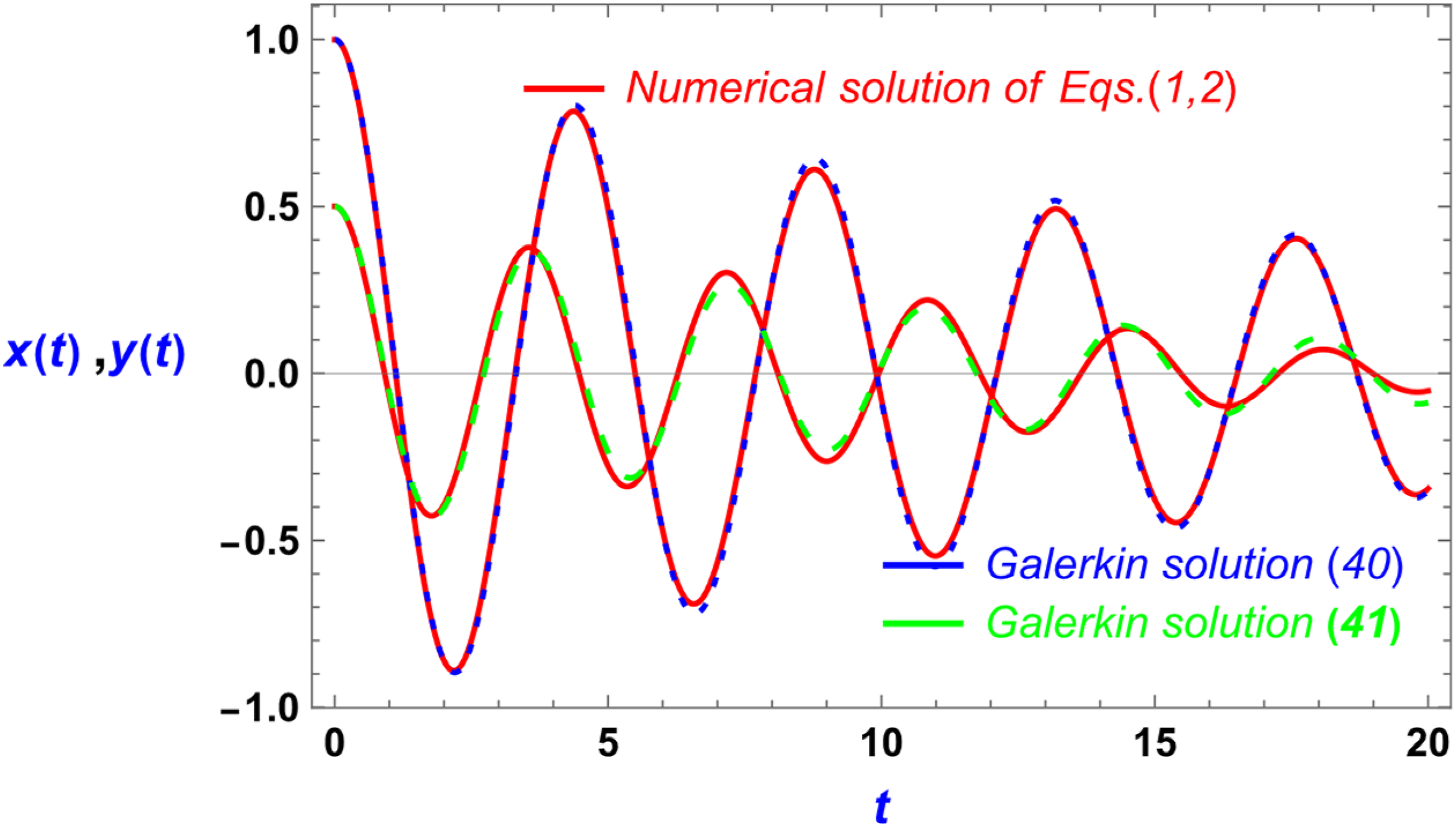

Figure 2.

Shows a comparison between the analytical solutions produced using the Galerkin approximation approach and the numerical solutions of the original equations (1) and (2) for the system having $A=1,B=0.5,{\mu }_{11}=0.1,{\mu }_{21}=0.001,{\mu }_{22}=0.2,{\mu }_{12}=0.0005,a_{11}=2,a_{21}=0.02,a_{22}=3,a_{12}=0.01,p_{11}=0.01,p_{21}=0.01,p_{22}=0.01,p_{12}=0.01,q_{11}=0.1,q_{21}=0.1,q_{22}=0.1,q_{12}=0.1,\omega =3$ .

The interaction of damping and the frequencies determines the linked system’s stability characteristic. Stability is ensured when system frequencies remain genuine and dampening is adequate to suppress oscillatory growth. Weak coupling results in relatively independent dynamics for each variable, whereas strong coupling can produce complicated interactions, potentially leading to resonant amplification of oscillations. Stability needs genuine coefficient damping rates ${\alpha }_j>0$ , ${\beta }_j>0$ , and system frequencies ( ${\mathrm{\Theta }}_{1j}^2$ >0 and ${\mathrm{\Theta }}_{2j}^2$ >0). When these conditions are met, the system remains stable, with actual frequencies and damping rates that govern oscillatory or exponential decay behavior while preventing unlimited growth or instability. The following requirements apply:

${\mathbb{C}}_1\left({\alpha }_j,{\beta }_j,{\Theta }_{1j},{\Theta }_{2j}\right)={\sigma }_{22}^2\left({\mu }_{11}{\sigma }_{22}^2-{\mu }_{12}{\sigma }_{21}^2\right)\left(4{\sigma }_{22}^2\left({\sigma }_{11}^2{\sigma }_{22}^2-{\sigma }_{12}^2{\sigma }_{21}^2\right)-{\left({\mu }_{11}{\sigma }_{22}^2-{\mu }_{12}{\sigma }_{21}^2\right)}^2\right)>0,$

(42)

${\mathbb{C}}_2\left({\alpha }_j,{\beta }_j,{\Theta }_{1j},{\Theta }_{2j}\right)={\sigma }_{11}^2\left({\mu }_{22}{\sigma }_{11}^2-{\mu }_{21}{\sigma }_{12}^2\right)\left(4{\sigma }_{11}^2\left({\sigma }_{11}^2{\sigma }_{22}^2-{\sigma }_{12}^2{\sigma }_{21}^2\right)-{\left({\mu }_{22}{\sigma }_{11}^2-{\mu }_{21}{\sigma }_{12}^2\right)}^2\right)>0,$

(43)

${\mathbb{C}}_3\left({\alpha }_j,{\beta }_j,{\Theta }_{1j},{\Theta }_{2j}\right)={\sigma }_{12}^2{\sigma }_{22}^2\left({\mu }_{11}{\sigma }_{12}^2-{\mu }_{12}{\sigma }_{11}^2\right)\left(4{\sigma }_{12}^4\left({\sigma }_{11}^2{\sigma }_{22}^2-{\sigma }_{12}^2{\sigma }_{21}^2\right)-{\sigma }_{22}^2{\left({\mu }_{11}{\sigma }_{12}^2-{\mu }_{12}{\sigma }_{11}^2\right)}^2\right)>0,$

(44)

${\mathbb{C}}_4\left({\alpha }_j,{\beta }_j,{\Theta }_{1j},{\Theta }_{2j}\right)={\sigma }_{11}^2{\sigma }_{21}^2\left({\mu }_{22}{\sigma }_{21}^2-{\mu }_{21}{\sigma }_{22}^2\right)\left(4{\sigma }_{21}^4\left({\sigma }_{11}^2{\sigma }_{22}^2-{\sigma }_{12}^2{\sigma }_{21}^2\right)-{\sigma }_{11}^2{\left({\mu }_{22}{\sigma }_{21}^2-{\mu }_{21}{\sigma }_{22}^2\right)}^2\right)>0.$

(45)

When these criteria are met, the system frequencies stay genuine, indicating a stable and physically meaningful system.

The transition curve, delineating stable and unstable states, is typically derived as a function of system parameters through comprehensive stability analysis. This function may be expressed as:

$\mathbb{C}\left({\alpha }_j,{\beta }_j,{\Theta }_{1j},{\Theta }_{2j}\right)=0,$

(46)

where $\mathbb{C}={\mathbb{C}}_1{\mathbb{C}}_2{\mathbb{C}}_3{\mathbb{C}}_4.$ represents the relationship between the system’s governing parameters that define the boundary separating stable and unstable regions.

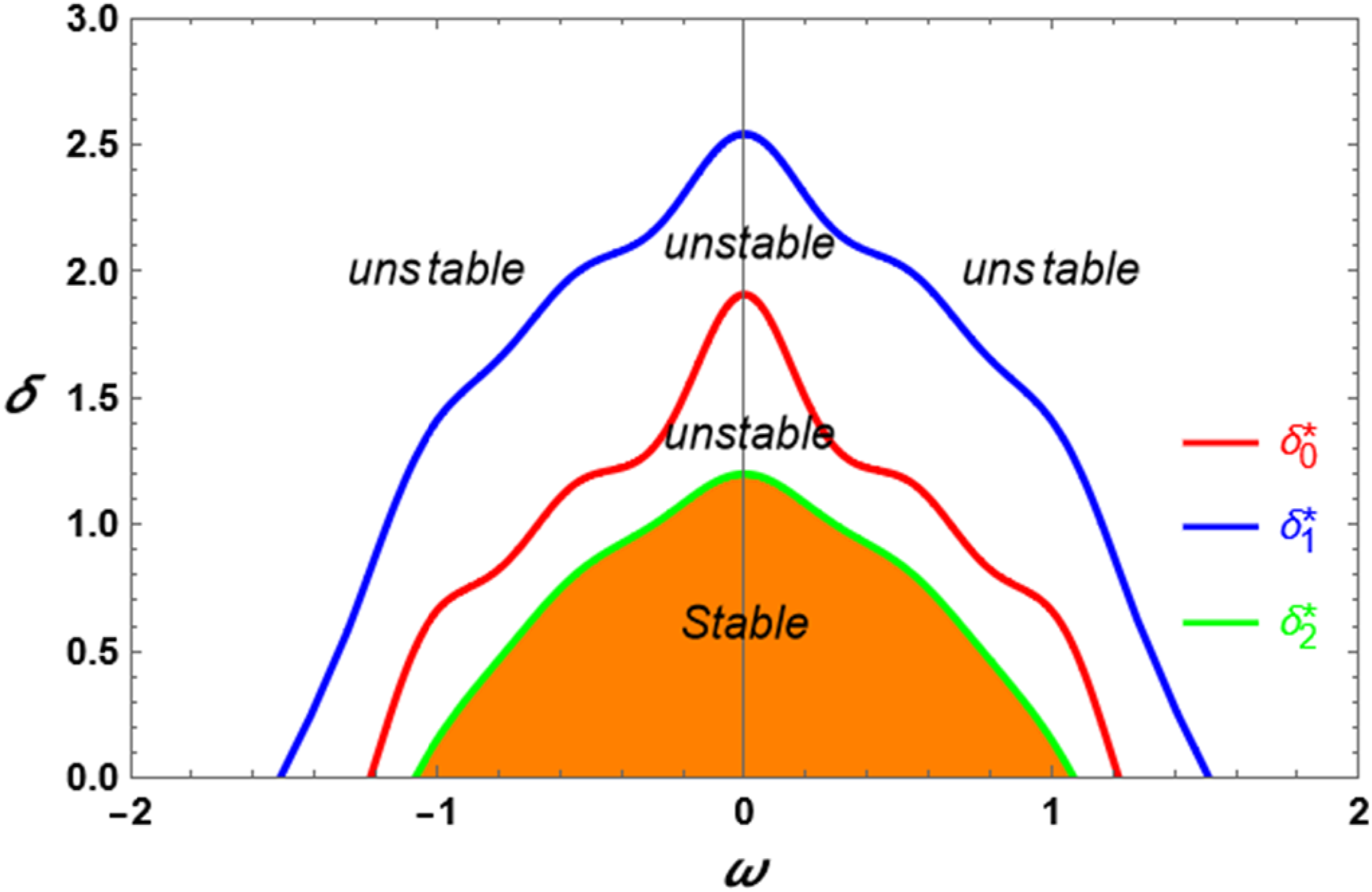
The transition curves in Figure 3 represent the relationship between the periodic force’s frequency and the product of the system’s intrinsic frequencies, as computed by (46). The graph depicts how the excitation frequency influences system dynamics, including the stability barrier. The system’s numerical parameters are selected as: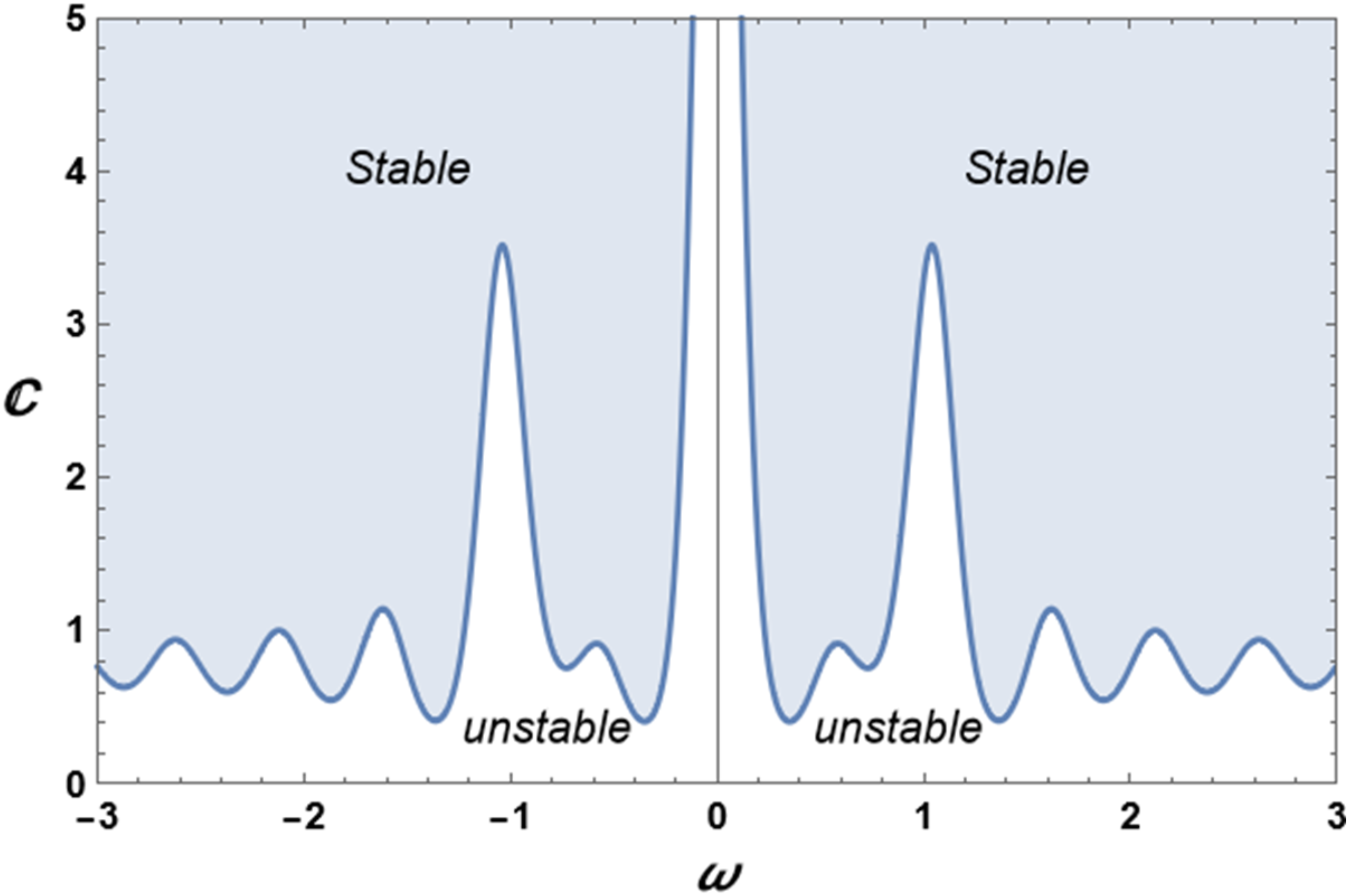

$A=1,B=0.5,{\mu }_{11}=0.1,{\mu }_{21}=0.001,{\mu }_{22}=0.2,{\mu }_{12}=0.0005,a_{11}=2,a_{21}=0.02,a_{22}=3,a_{12}=0.01,p_{11}=0.01,p_{21}=0.01,p_{22}=0.01,p_{12}=0.01,q_{11}=0.1,q_{21}=0.1,q_{22}=0.1,q_{12}=0.1,\omega =3.$

Figure 3.

Graphing the stability conditions (42)–(45).

The graph depicts the plane ( $\mathbb{C}-\omega$ ) as separated into two distinct regions: a stable region above the transition curve and an unstable region underneath it. The transition curve shows a sequence of peaks and troughs, with the lowest dip being near ω = 0. A shallower trough occurs at ω = 1, followed by a series of peaks and troughs as ω goes away from ω = ±1. The pattern illustrates the excitation frequency’s alternating stabilizing and destabilizing effects. This pattern decays with increasing ω. The strongest destabilizing effects are seen at ω = 0 and ω = ±1, when peaks and troughs are most noticeable.

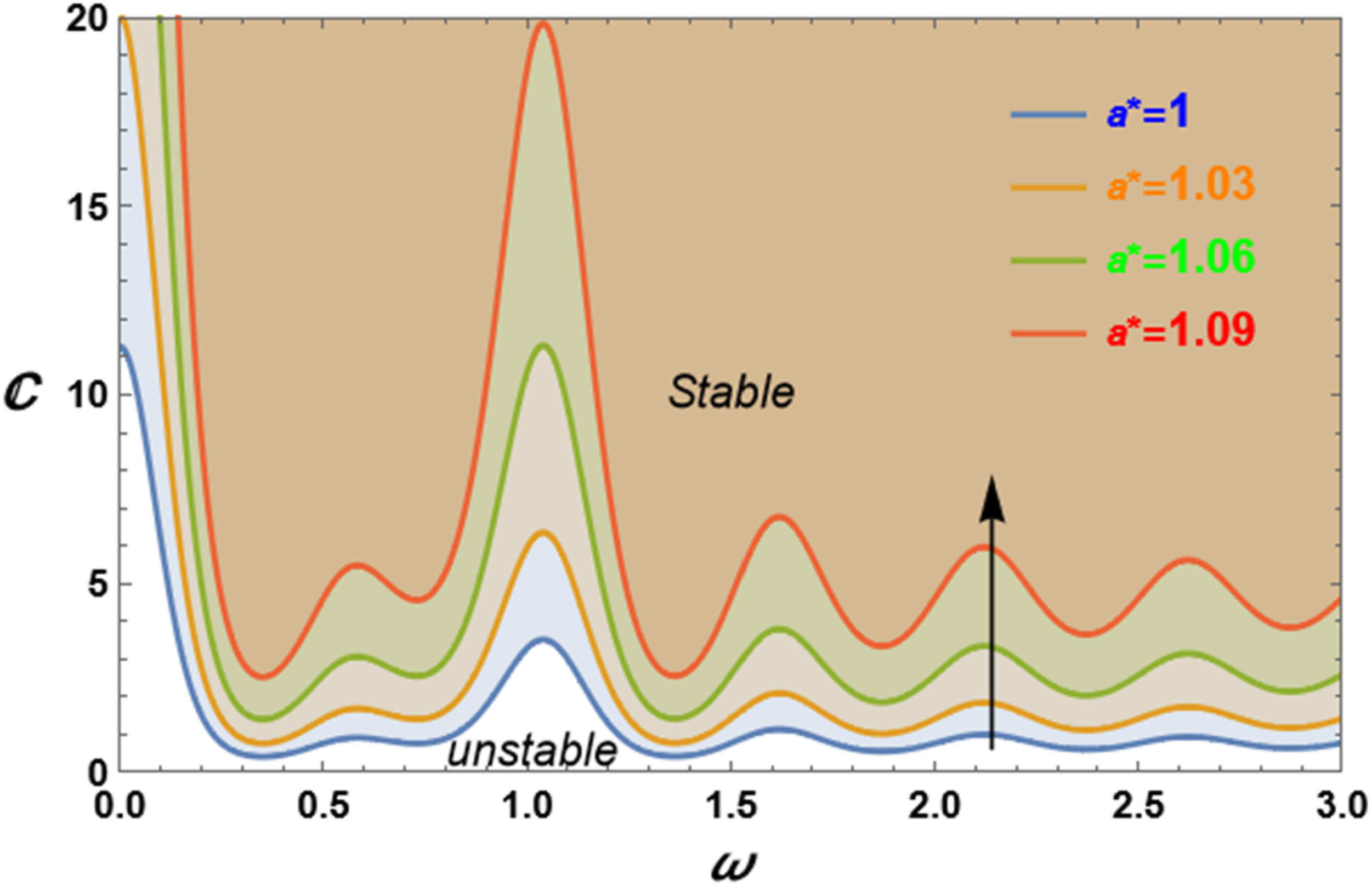
Figure 4 shows the effect of the four damping coefficients. The examination involves increasing the four coefficients by a factor denoted by μ* while holding the other components constant, as shown in Figure 3. As μ*increases somewhat, the stable zone shifts upward, indicating a destabilizing impact from raising the damping coefficients together. A similar behavior is observed when the four coefficients of the constant natural frequencies are increased simultaneously, as illustrated in Figure 5, and when the four excitation amplitudes are slightly increased together, as depicted in Figure 6.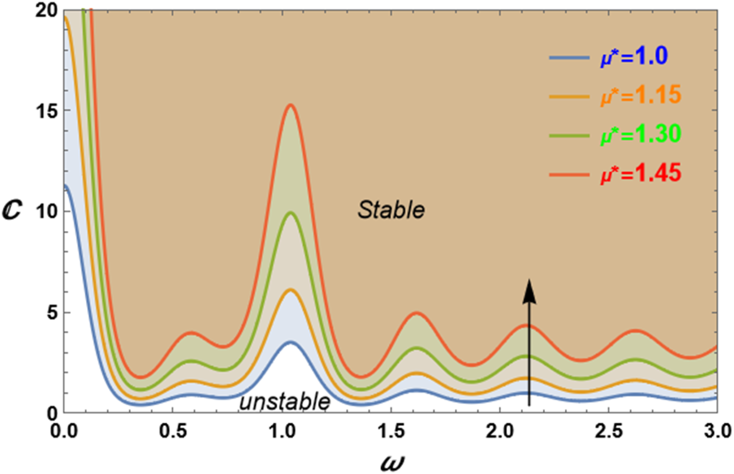

Figure 4.

Graphing the stability conditions (42)–(45) for the variation of the damping coefficients ${\mu }^{*}{\mu }_{ij},$ for the same system considered in Figure 3.

Figure 5.

Graphing the stability conditions (42)–(45) for the variation of the factor of the constant natural frequency coefficients $a^{*}{a}_{ij},$ for the same system considered in Figure 3.

Figure 6.

Graphing the stability conditions (42)–(45) for the variation of the damping coefficients $q^{*}{q}_{ij},$ for the same system considered in Figure 3.

Galerkin method and the parametric resonant case

The approach of ${\mathrm{\Theta }}_2$ ​ to the parametric frequency ω can be expressed by introducing a small-parameter δ, which quantifies the deviation between ${\mathrm{\Theta }}_2$ ​ and ω. This can be defined as:

${\Theta }_2^2={\omega }^2+\delta ,$

(47)

where δ is a small parameter that represents the difference between the frequency ${\mathrm{\Theta }}_2$ ​​ and the parametric frequency ω, allowing for an approximation around the resonance condition. The parameter δ serves as a control variable to investigate near-resonance effects, enabling a detailed analysis of the system’s dynamic response under almost resonant conditions. It is noteworthy that a similar strategy can be employed when ${\mathrm{\Theta }}_1$ approaches the parametric frequency ω.

Substituting equation (47) into (32)–(35) and simplifying as previously explained, the mathematical analysis leads to two sets of solutions, one of them satisfied at the non-resonance case, which is identical to the results given in (36), and the second set of solutions that controls the behavior at the parametric resonance, which is given as

$r_4{\Theta }_1^4+r_2{\Theta }_1^2+r_0=0,$

(48)

where

$r_4=4\left({\sigma }_{11}^2{\sigma }_{22}^2-{\sigma }_{12}^2{\sigma }_{21}^2\right)-\left(4\delta +4{\omega }^2+{\mu }_{22}^2\right){\sigma }_{11}^2,$

(49)

$r_2=-2{\mu }_{21}{\mu }_{22}{\sigma }_{11}^2{\sigma }_{12}^2+\frac{1}{2{\sigma }_{22}^4}\left(\left({\mu }_{22}^2+4\delta +4{\omega }^2\right){\sigma }_{11}^2-4\left({\sigma }_{11}^2{\sigma }_{22}^2-{\sigma }_{12}^2{\sigma }_{21}^2\right)\right)\times \left(\left({\mu }_{12}{\sigma }_{21}^2+2{\mu }_{11}{\sigma }_{22}^2\right){\mu }_{12}{\sigma }_{21}^2+\left(4{\sigma }_{11}^2-{\mu }_{11}^2\right){\sigma }_{22}^4\right),$

(50)

$r_0=-\frac{1}{16{\sigma }_{22}^8}{\left({\left({\mu }_{12}{\sigma }_{21}^2-{\mu }_{11}{\sigma }_{22}^2\right)}^2-4{\sigma }_{11}^2{\sigma }_{22}^4\right)}^2\left(\left({\mu }_{22}^2+4\delta +4{\omega }^2\right){\sigma }_{11}^2-4\left({\sigma }_{11}^2{\sigma }_{22}^2-{\sigma }_{12}^2{\sigma }_{21}^2\right)\right)-\frac{{\mu }_{21}{\sigma }_{11}^2{\sigma }_{12}^2}{2{\sigma }_{22}^4}\left(2{\sigma }_{22}^4\left({\mu }_{21}{\sigma }_{12}^2-2{\mu }_{22}{\sigma }_{11}^2\right)+{\mu }_{22}{\left({\mu }_{12}{\sigma }_{21}^2-{\mu }_{11}{\sigma }_{22}^2\right)}^2\right).$

(51)

Further, the damping coefficient $\alpha$ is given by

$b_2{\alpha }^2-b_1\alpha +b_0=0,$

(52)

where

$b_2=4\left({\sigma }_{22}^2-\delta -{\omega }^2\right)-{\mu }_{22}^2,$

(53)

$b_1=4{\mu }_{11}\left(\delta +{\omega }^2-{\sigma }_{22}^2\right)+\left({\mu }_{11}{\mu }_{22}-{\mu }_{12}{\mu }_{21}\right){\mu }_{22}+2{\mu }_{12}{\sigma }_{21}^2,$

(54)

$b_0=\left({\sigma }_{22}^2-\delta -{\omega }^2\right){\mu }_{11}^2-\frac{1}{4}{\left({\mu }_{12}{\mu }_{21}-{\mu }_{11}{\mu }_{22}\right)}^2-{\mu }_{11}{\mu }_{12}{\sigma }_{21}^2.$

(55)

The stability constraint that needs to be satisfied at the parametric resonance is the frequency ${\Theta }_1^2$ must be real and positive, as well as the damping coefficient $\alpha$ . The positivity can be satisfied when $r_4>0,r_2<0,r_0>0,b_2>0,b_1>0,$ and $b_0>0$ . In addition, the discriminant of both (48) and (52) must be positive to ensure the reality which has the following arrangement:

$\delta <{\delta }_0^{*}=\frac{{\sigma }_{21}^4+{\mu }_{21}^2{\sigma }_{22}^2-{\mu }_{21}{\mu }_{22}{\sigma }_{21}^2-{\mu }_{21}^2{\omega }^2}{{\mu }_{21}^2},$

(56)

$c_2{\delta }^2-c_1\delta +c_0>0,$

(57)

These conditions ensure that the roots of the governing equations (48) and (52) remain real and bounded, which is essential for stability in the parametric resonance scenario. It is noted that condition (40) can be satisfied when

$\delta >{\delta }_1^{*}\cup \delta <{\delta }_2^{*},$

(58)

where ${\delta }_1^{*}>{\delta }_2^{*}$ which are given by

${\delta }_1^{*}=\frac{1}{2c_2}\left(c_1+\sqrt{c_1^2-4c_0{c}_2}\right),\text{and}{\delta }_2^{*}=\frac{1}{2c_2}\left(c_1-\sqrt{c_1^2-4c_0{c}_2}\right),$

(59)

$c_2=64{\mu }_{12}^2{\sigma }_{11}^4{\sigma }_{21}^4{\sigma }_{22}^2\left(2{\mu }_{11}{\mu }_{12}{\sigma }_{21}^2-{\mu }_{11}^2{\sigma }_{22}^2+4{\sigma }_{11}^2{\sigma }_{22}^2\right),$

(60)

$c_1=32{\sigma }_{11}^2{\sigma }_{22}^2\left\{\begin{array}{l}{\mu }_{12}^2{\sigma }_{21}^4\left({\sigma }_{11}^2\left(4{\omega }^2+{\mu }_{22}^2\right)-4\left({\sigma }_{11}^2{\sigma }_{22}^2-{\sigma }_{12}^2{\sigma }_{21}^2\right)\right)\left({\mu }_{11}^2{\sigma }_{22}^2-2{\mu }_{11}{\mu }_{12}{\sigma }_{21}^2-4{\sigma }_{11}^2{\sigma }_{22}^2\right)\\ +2{\mu }_{21}{\sigma }_{11}^2{\sigma }_{22}^2{\sigma }_{12}^2\left({\mu }_{21}{\sigma }_{12}^2{\sigma }_{22}^4+{\mu }_{12}^2{\mu }_{22}{\sigma }_{21}^4\right)\end{array}\right\},$

(61)

$c_0={\left(\begin{array}{l}\left({\mu }_{12}{\sigma }_{21}^2\left({\mu }_{12}{\sigma }_{21}^2+2{\mu }_{11}{\sigma }_{22}^2\right)-\left({\mu }_{11}^2-4{\sigma }_{11}^2\right){\sigma }_{22}^4\right)\left({\sigma }_{11}^2\left(4{\omega }^2+{\mu }_{22}^2\right)-4\left({\sigma }_{11}^2{\sigma }_{22}^2-{\sigma }_{12}^2{\sigma }_{21}^2\right)\right)\\ -4{\mu }_{21}{\mu }_{22}{\sigma }_{11}^2{\sigma }_{12}^2{\sigma }_{22}^4\end{array}\right)}^2$

$-{\left({\sigma }_{11}^2\left(4{\omega }^2+{\mu }_{22}^2\right)-4\left({\sigma }_{11}^2{\sigma }_{22}^2-{\sigma }_{12}^2{\sigma }_{21}^2\right)\right)}^2{\left(-4{\sigma }_{11}^2{\sigma }_{22}^4+{\left({\mu }_{12}{\sigma }_{21}^2-{\mu }_{11}{\sigma }_{22}^2\right)}^2\right)}^2$

$+8{\mu }_{21}{\sigma }_{11}^2{\sigma }_{12}^2{\sigma }_{22}^4\left({\sigma }_{11}^2\left(4{\omega }^2+{\mu }_{22}^2\right)-4\left({\sigma }_{11}^2{\sigma }_{22}^2-{\sigma }_{12}^2{\sigma }_{21}^2\right)\right)\times \left(2\left(2{\mu }_{22}{\sigma }_{11}^2-{\mu }_{21}{\sigma }_{12}^2\right){\sigma }_{22}^4-{\mu }_{22}{\left({\mu }_{12}{\sigma }_{21}^2-{\mu }_{11}{\sigma }_{22}^2\right)}^2\right).$

(62)

Combining the stability conditions (46) and (48) yields the stability criteria in the form.

$\left(\delta >{\delta }_1^{*}\cap \delta <{\delta }_0^{*}\right)\cup \left(\delta <{\delta }_2^{*}\cap \delta <{\delta }_0^{*}\right),$

(63)

This analysis highlights the delicate balance between excitation frequency, damping coefficients, and nonlinearity required to achieve stability in the parametric resonance case.

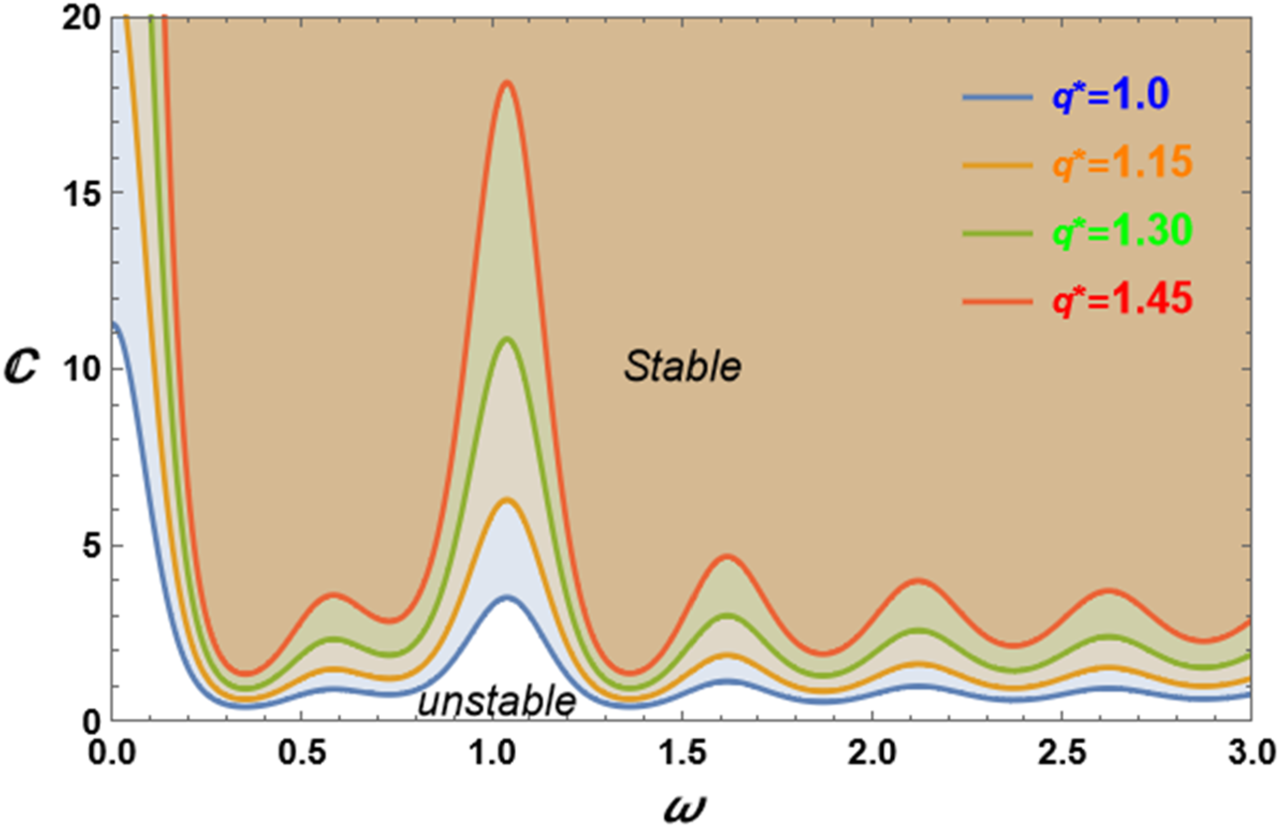
Figure 7 depicts the stability behavior at parametric resonance, as described by the stability requirement in equation (46). The system’s numerical values are chosen as $A=B=0.1,{\mu }_{11}=0.5,{\mu }_{22}=0.3,{\mu }_{12}={\mu }_{21}=0.01,a_{11}=a_{22}=1,a_{21}=a_{12}=0.01,p_{11}=p_{21}=p_{22}=p_{12}=0.01,q_{11}=q_{21}=q_{22}=q_{12}=0.01.$

In this graph, the red curve corresponds to the transition curve described by equation (56), which serves as the primary stability criterion, while the blue and green curves represent the transition curves given in equation (59). The orange-shaded region highlights the stable domain under resonance conditions. Conversely, the unshaded area indicates a non-resonant unstable region, whereas the narrow white band within the orange region denotes instability arising specifically from parametric resonance. This visualization effectively delineates the interplay between resonance and stability across different parameter ranges.

Figure 7.

Shows the parametric resonance region demonstrated by condition (51).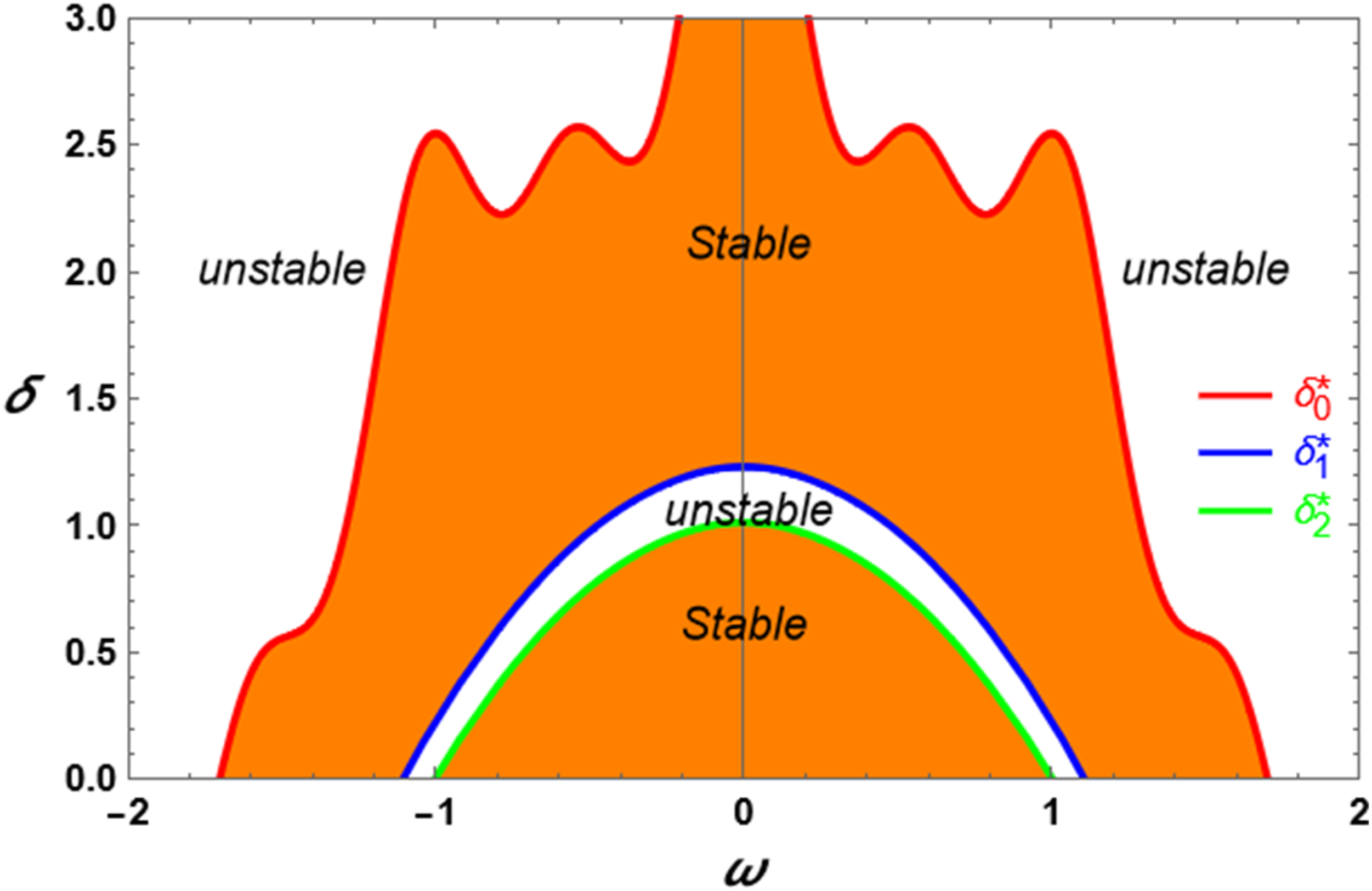

When the damping coefficient 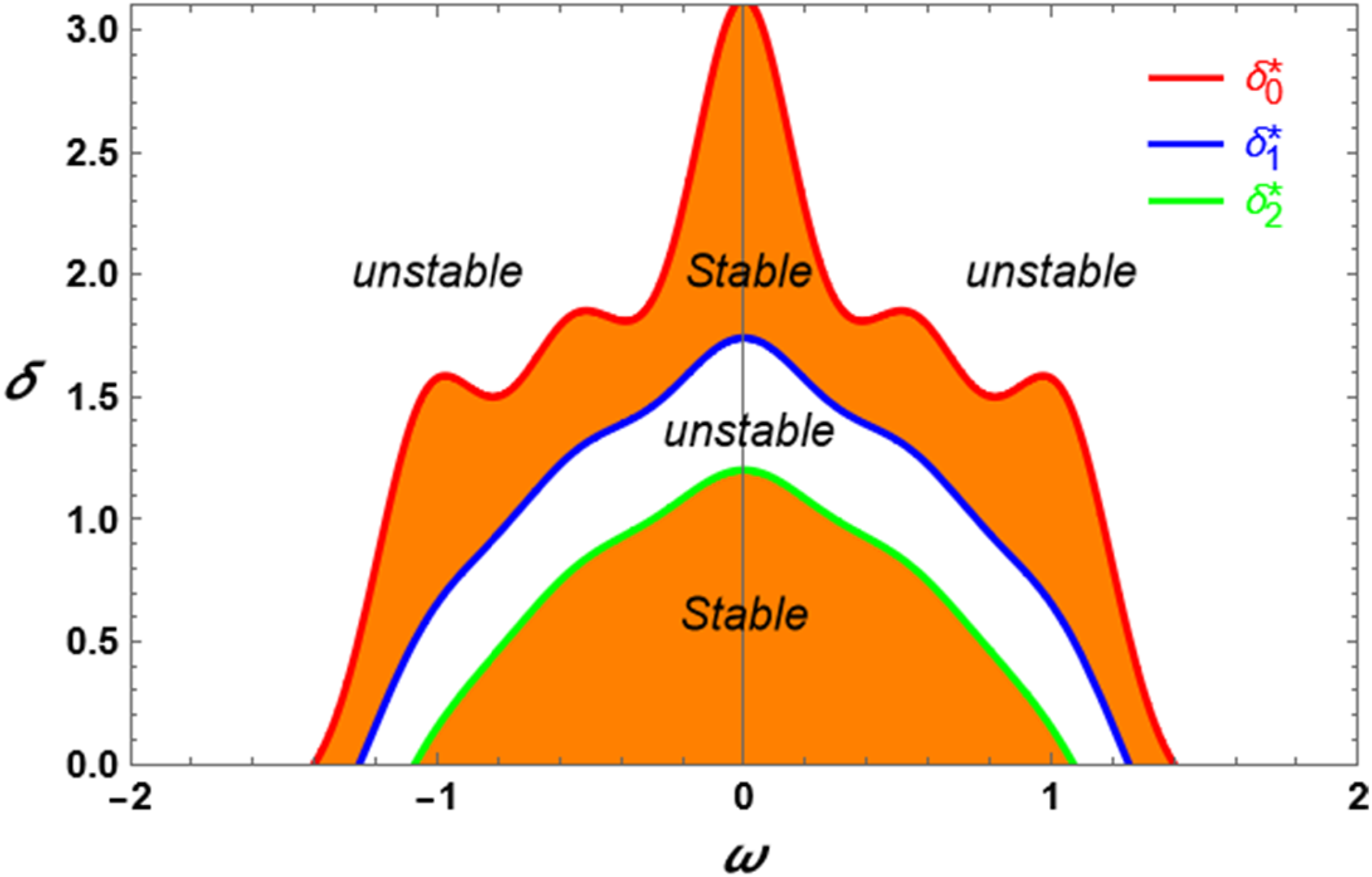${\mu }_{21}$ is slightly increased to a new value ${\mu }_{21}=0.013$ , the resulting stability behavior is depicted in Figure 8. In this graph, the shaded orange region, representing the stable domain, decreases, while the unshaded regions expand. This change is accompanied by a widening of the unstable resonance region, indicating an increased instability effect due to the higher damping coefficient ${\mu }_{21}$ . This behavior demonstrates the destabilizing effect of rising ${\mu }_{21}$ as an example on the system’s overall stability. As the coefficient ${\mu }_{21}$ is increased to a new value ${\mu }_{21}=0.02.$ , the critical transition curve defined by equation (46) shifts downward, entering the unstable resonance region, as shown in Figure 9. At this stage, the stability condition outlined in equation (61) results in the formation of a small stable zone, depicted as the shaded orange region. This demonstrates the influence of increasing ${\mu }_{21}$ or reducing the overall stability area while emphasizing the emergence of localized stability within the unstable resonance domain.

Figure 8.

Shows the parametric resonance region demonstrated by condition (61) for the same system given in Figure 7 except that ${\mu }_{21}=0.013$ .

Figure 9.

Shows the parametric resonance region demonstrated by conditions (61) for the same system given in Figure 7 except that. ${\mu }_{21}=0.02$ .

Galerkin method and internal resonance structure

In this section, we address the resonant case where the frequency ${\mathrm{\Theta }}_2$ approaches the frequency ${\mathrm{\Theta }}_1$ . This proximity can be characterized by introducing a small dimensionless parameter ε (ε≪1), defined as:

${\mathrm{\Theta }}_2={\mathrm{\Theta }}_1+\epsilon .$

(64)

Employing equation (64) into the characteristic equation (27) and making use the substitutions $\alpha =\beta$ → $\nu$ , while utilizing trigonometric identities, equation (27) can be systematically rearranged to simplify its components, making it more interpretable for applying the Galerkin approach

$C^{-}\hspace{0.17em}\mathit{cos}\left(\epsilon t\right)+C^{+}\hspace{0.17em}\mathit{cos}\left(2{\Theta }_1+\epsilon \right)t-S^{-}\hspace{0.17em}\mathit{sin}\left(\epsilon t\right)+S^{+}\hspace{0.17em}\mathit{sin}\left(2{\Theta }_1+\epsilon \right)t=0,$

(65)

where

$C^{\mp }=\mp \left({\nu }^2+{\Theta }_1^2\right){\mu }_{12}\left(\left({\nu }^2+{\left(\epsilon +{\Theta }_1\right)}^2\right){\mu }_{21}-\nu {\sigma }_{21}^2\right)\pm \nu \left({\nu }^2+{\left(\epsilon +{\Theta }_1\right)}^2\right){\mu }_{21}{\sigma }_{12}^2\mp \left({\nu }^2\pm {\Theta }_1\left(\epsilon +{\Theta }_1\right)\right){\sigma }_{12}^2{\sigma }_{21}^2,$

(66)

$S^{\mp }={\Theta }_1^2\left(\epsilon +{\Theta }_1\right){\mu }_{12}{\sigma }_{21}^2+\nu \left(\epsilon +{\Theta }_1\right)\left(\nu {\mu }_{12}-{\sigma }_{12}^2\right){\sigma }_{21}^2\mp {\Theta }_1{\sigma }_{12}^2\left(\left({\nu }^2+{\left(\epsilon +{\Theta }_1\right)}^2\right){\mu }_{21}-\nu {\sigma }_{21}^2\right).$

(67)

The Galerkin method provides a systematic way to approximate ε by leveraging orthogonal basis functions and weighted residuals. Applying this technique to equation (65), based on the chosen basis functions, yields

${\int }_0^{2\pi /s}\hspace{0.5em}\left(C^{-}\hspace{0.17em}{\cos }^2\left(\epsilon t\right)-S^{-}\hspace{0.17em}{\sin }^2\left(\epsilon t\right)\right)\mathrm{d}t=0$

(68)

${\int }_0^{2\pi /\left(2{\mathrm{\Theta }}_1+\epsilon \right)}\hspace{0.5em}\left(C^{+}\hspace{0.17em}{\cos }^2\left(2{\mathrm{\Theta }}_1+\epsilon \right)t+S^{+}\hspace{0.17em}{\sin }^2\left(2{\mathrm{\Theta }}_1+\epsilon \right)t\right)\mathrm{d}t=0$

(69)

Based on the definitions given in (65) and (67), equations (68) and (69) provided the following equations that related the unknown $\nu$ with the small parameter $\epsilon$ and the frequency ${\Theta }_1$ :

$\left({\nu }^2+{\Theta }_1^2\right){\mu }_{12}\left(-\left(\left({\epsilon }^2+{\nu }^2+2\epsilon {\Theta }_1+{\Theta }_1^2\right){\mu }_{21}\right)+\left(\epsilon +\nu +{\Theta }_1\right){\sigma }_{21}^2\right)+{\sigma }_{12}^2\left(\left(\nu -{\Theta }_1\right)\left({\epsilon }^2+{\nu }^2+2\epsilon {\Theta }_1+{\Theta }_1^2\right){\mu }_{21}-\left(\nu \left(\epsilon +\nu \right)+{\Theta }_1\left(\epsilon +{\Theta }_1\right)\right){\sigma }_{21}^2\right)=0,$

(70)

$\left({\nu }^2+{\Theta }_1^2\right){\mu }_{12}\left(\left({\epsilon }^2+{\nu }^2+2\epsilon {\Theta }_1+{\Theta }_1^2\right){\mu }_{21}+\left(\epsilon -\nu +{\Theta }_1\right){\sigma }_{21}^2\right)+{\sigma }_{12}^2\left(-\left(\left(\nu -{\Theta }_1\right)\left({\epsilon }^2+{\nu }^2+2\epsilon {\Theta }_1+{\Theta }_1^2\right){\mu }_{21}\right)-\left(\left(\epsilon -\nu \right)\nu +{\Theta }_1\left(\epsilon +2\nu +{\Theta }_1\right)\right){\sigma }_{21}^2\right)=0.$

(71)

An expression between the small parameter $\epsilon$ and ${\mathrm{\Theta }}_1$ can be achieved by eliminating the damping coefficient $\nu$ between equations (70) and (71) which yields

${\lambda }_2{\Theta }_1^2+{\lambda }_1{\Theta }_1+{\lambda }_0=0,$

(72)

where the coefficients ${\lambda }_2,{\lambda }_1$ , and ${\lambda }_0$ are listed below:

${\lambda }_2={\left({\mu }_{21}{\sigma }_{12}^2-{\mu }_{12}{\sigma }_{21}^2\right)}^2+{\mu }_{21}^2{\left({\sigma }_{12}^2+2\epsilon {\mu }_{12}\right)}^2,$

(73)

${\lambda }_1=4{\epsilon }^3{\mu }_{12}^2{\mu }_{21}^2+{\mu }_{21}{\sigma }_{12}^4\left(2\epsilon {\mu }_{21}+{\sigma }_{21}^2\right)+{\mu }_{12}{\sigma }_{12}^2\left(2{\epsilon }^2{\mu }_{21}^2-2\epsilon {\mu }_{21}{\sigma }_{21}^2-{\sigma }_{21}^4\right),$

(74)

${\lambda }_0={\epsilon }^2{\mu }_{21}\left({\epsilon }^2{\mu }_{12}^2{\mu }_{21}+{\mu }_{21}{\sigma }_{12}^4-{\mu }_{12}{\sigma }_{12}^2{\sigma }_{21}^2\right).$

(75)

To ensure that the stability criteria are satisfied, the frequency ${\mathrm{\Theta }}_1$ must be a real quantity. This condition can be achieved when the discriminant of the quadratic equation derived from equation (71) is positive. Mathematically, this can be expressed as follows:

$4{\epsilon }^2{\mu }_{21}^2{\left(\epsilon {\mu }_{12}+{\sigma }_{12}^2\right)}^2-4\epsilon {\mu }_{21}{\sigma }_{12}^2{\sigma }_{21}^2\left(\epsilon {\mu }_{12}+{\sigma }_{12}^2\right)-{\sigma }_{12}^4{\sigma }_{21}^4<0.$

(76)

This condition provides a straightforward mathematical requirement for ensuring the stability of the system, where ${\mathrm{\Theta }}_1$ remains a real quantity. Insert the real roots of equality of condition (76) into equation (64) using the roots of (61) the transition curves can be sought in the form

${\Theta }_{2j}=\frac{1}{2{\lambda }_2}\left(-{\lambda }_1\pm \sqrt{{\lambda }_1^2-4{\lambda }_0{\lambda }_2}\right)+{\epsilon }_j,$

(77)

where ${\epsilon }_j$ refers to real roots of the equality of condition (76).

Using the system’s numerical values from Figure 7 in the transition curve corresponding to the stability condition (76) yields two distinct transition curves. Consequently, the curves defined by equation (77) have been plotted in Figure 10. This graph illustrates the stability behavior under the internal resonance condition. The orange-shaded region represents the stable domain, while the unshaded region indicates the unstable resonance domain, highlighting the system’s dynamic response to internal resonance conditions.

Figure 10.

Graphing of the internal resonance region given by (77).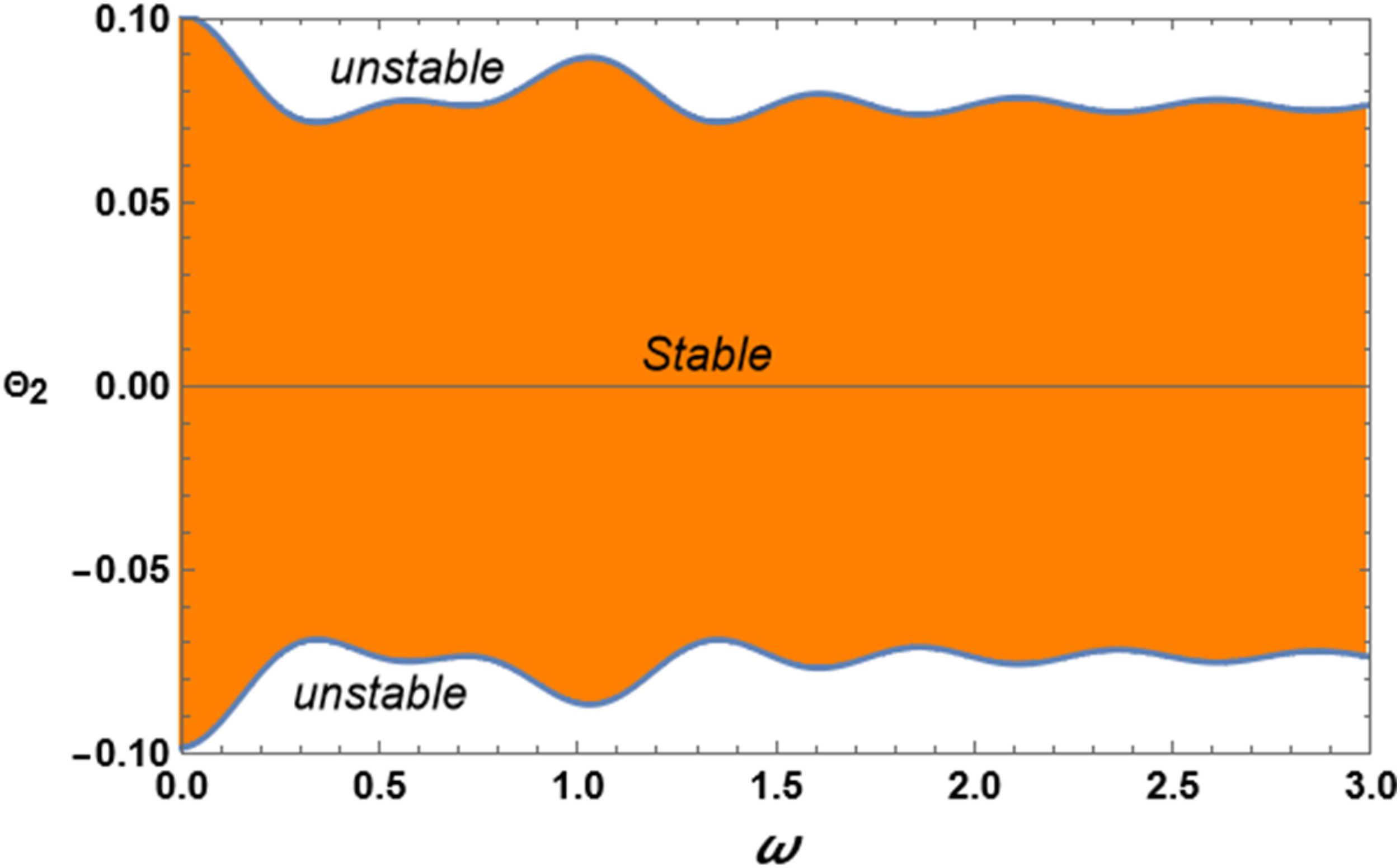

Conclusion

The study showcases the effectiveness of using the renormalization approach alongside the Galerkin method for analyzing the stability of two nonlinear Mathieu oscillators, offering a more comprehensive evaluation of nonlinear dynamics without weak constraints. The renormalized approach simplifies system features while preserving mathematical complexity, enabling accurate analysis of stability boundaries, resonance interactions, and parametric influences, aligning with classical perturbation techniques, and offering modern flexibility. The study uses the Galerkin method and renormalization-based transformation to study the stability of two nonlinear Mathieu oscillators, simplifying mathematical treatment and allowing direct evaluation of stability boundaries and resonance conditions under periodic forcing. The study explores stability behavior in internal and parametric resonances, revealing the intricate interplay of nonlinear coupling and periodic excitation, using the Galerkin approach for analytical clarity and computational feasibility. The Galerkin technique’s versatility in renormalized and autonomous settings provides insights for mechanical systems, MEMS devices, and vibrational stability control, laying the groundwork for future studies. Overall, this method strengthens our ability to analyze and control nonlinear dynamic behavior in engineering, physics, and MEMS applications, laying a solid foundation for future research in coupled oscillators and advanced stability modeling.