Sage Journals: Discover world-class research

Abstract

The present study emphasizes an optimized deep learning algorithm for gearbox fault detection using vibration, sound, and acoustic emission signals. Statistical and acoustic features are extracted from these signals, and various neural network algorithms are explored. The supervised deep feed forward neural network (DFFNN) demonstrates excellent performance with vibration signals but limited accuracy with sound and acoustic emission signals. To address this, unsupervised algorithms are optimized and compared with vibration-based classification. The findings show that unsupervised neural networks, particularly the auto-encoder and stacked auto-encoder architectures, achieve improved classification accuracy by leveraging the unique characteristics of acoustic emission signals. The unsupervised models also effectively overcome the vanishing gradient problem via regularization, enhancing their training efficiency. The stacked auto-encoder, with multiple layers of encoders and decoders, reduces computation time by 40% and memory consumption. These optimized algorithms hold promise for automated fault detection systems. The auto-encoder and stacked auto-encoder, utilizing vibration, sound, and acoustic emission signals, offer enhanced classification accuracy and can facilitate real-time monitoring of rotating mechanical systems. However, further optimization is needed to maximize their performance. In a nutshell, the supervised DFFNN excels in utilizing vibration signals for fault detection, while the unsupervised models exploit the distinctive characteristics of acoustic emission signals. Future research will focus on refining these algorithms to enhance their effectiveness. Implementing these optimized deep learning approaches can lead to autonomous fault detection systems, eliminating the need for continuous human supervision.

Keywords

Gearbox fault diagnosis deep learning vibration signal sound signal acoustic emission signal feature extraction stacked auto- encoders

Introduction

Automobiles provide an easy and comfortable commute, which is necessary for daily life. The increased population and finite resources have demanded the implementation of Hybrid Electric Vehicles (HEV) and Electric Vehicles (EVs). The HEVs are the perfect balance between combustion and electric vehicles, where the HEVs use an electric motor for torque applications and an IC engine for high-speed applications.¹ Using multiple power sources demands complex rotational systems such as gearboxes, responsible for varying gear ratios to achieve higher speed without compromising initial torque.² The extreme working conditions of the gearbox lead to pitting, wear, misalignment, and specific other faults in their gears and bearings. This will lead to lesser efficiency and increased friction on the gears and bearings, even with proper lubrication.³

The excessive use of the gearbox will induce stress extending over the Factor of Safety (FOS), causing deterioration of gears such as tooth break and tooth wear, pitting, scuffing, cracking, bearing wear, noise, and vibration.⁴ Thus, the rotating machinery’s critical failures and health had to be detected to avoid significant failure and accidents.⁵ Along with the gears, the gearbox bearings are also suspected of high bending and axial load and are commonly diagnosed using vibration analysis.⁶ The vibration analysis can also be used for damage detection of multiple system components and condition-based monitoring of gears and bearings.⁷

The condition-based monitoring of the rotating systems is developed to utilize the condition indicator in the vibration signal acquired from the gearbox. The primary purpose of using vibration signals is to determine the dynamic characteristics of the gearbox.⁸ The vibration signals are produced by induced forces on the internal gears and bearing of the gearbox generated due to poor lubrication, gear pitting, bearing misalignment, etc.⁹ Literature studies have proved that the vibration signals are most efficient for fault detection and even the raw vibration signals are efficient in fault diagnosis of gears.^10–14 The cited literature data demonstrates that the higher dimension of vibration signals helps in the accurate and faster detection of faults compared to wear debris analysis. Besides vibration signals, the sound signals can also precisely detect faults in an early stage. The sound signals are also chosen for fault diagnosis as the sound analyzers are efficient with a wide bandwidth of microphones.¹⁵

The sound signals are the propagation of sound waves, and they contain information about the behavior and working conditions of the system it is exhibited from. The faults of a system produce sound with the respective characteristic frequency that can be used to determine the condition of any system. For instance, Mohanraj and Kumar¹⁶ used sound signals to predict the optimal processing condition of their tool in machining. Many non-intrusive methods using one or more microphones for condition monitoring of the internal combustion engine have been employed successfully and analyzed using machine learning techniques.¹⁷ Apart from vibration analysis, the shafts and bearings can be diagnosed by sound signal analysis and are often compared with vibration and motor current.^18,19 Thus, the degradation of a gearbox is followed by a gradual increase in sound upon aging; it can be used to determine the health of the gearbox by employing machine learning techniques. Even most medical diagnosis and analysis tools are subsonic and ultrasonic,²⁰ and the structural analysis of buildings is also done using sound signals.²¹ Although the vibration and sound signals accurately detect faults, early detection is necessary for some instances, which can be done using acoustic emission signals.

Acoustic Emission (AE) is the rapid release of energy on a system surface generated as propagating waves. These transient waves are released during any deformation on the tooth’s surface. The AE signals are emitted at a range of phenomena at every working condition and significantly affect the AE signals acquired, which can help detect faults in any system early.²² Ahn et al.²³ and Hou et al.²⁴ have proved that the signals are much more responsive to early detection of faults than vibration signals, even at bearing fault analysis. According to Van Hecke et al.,²⁵ the AE signals behave with instant changes in their dynamic responses compared to vibration signals. Such signals have higher sensitivity towards the location of faults and are immune to mechanical background noises. As the AE signals are predefined with acoustic features, extracting the features is unnecessary, making it easy for fault detection even at lower speeds.

Condition monitoring and fault detection involve data acquisition, data processing, and data classification to predict the health of the gearbox. The critical part of the data-driven degradation investigation is to extract the representative features from the acquired raw signal data. Praveenkumar et al.²⁶ classified the static features such as mean root square, Kurtosis, and acoustic features are extracted from the vibration signal and gearbox faults using machine learning algorithms. Kumar et al.²⁷ determined that the effectiveness of the input features can be improved by using multi-feature fusion techniques, which reduces the declassification of faults. Similarly, several different algorithms can be used for fault detection of any component to avoid future damage to that component and its associated systems. Various algorithms are proven efficient and compatible with different signals and their features.

One of the most efficient algorithms is the Support Vector Machine (SVM), which classifies the data by creating hyperplanes between the classes. The SVM algorithm can be trained at the highest and lowest speed conditions to define a range of suitable gearboxes.²⁸ The internal analysis methods can be varied by using different kernels, and the RBF kernel is claimed to be best suited with SVM for time-domain signals when compared with other kernels like linear, proximal, polynomial, and sigmoid.²⁹ The decision tree and SVM algorithm can be used for multi-component analysis and prove to have increased fault classification accuracy using RBF classification.³⁰ Apart from SVM, Artificial Neural Networks (ANN) are being used these days, which have better classification accuracy as the algorithm uses multiple neurons to learn from the unprocessed data. The rotating components, such as the rolling element bearings, can be diagnosed by Artificial Neural Network and are best suited for fault detection of rotating machines and online monitoring.³¹ The ANN algorithms are adopted as they can minimize the error in fault detection by updating the weight matrix on every iterative training, and a further improvement in classification can be made by employing multi-sensor fusion techniques.³² Any rotating component, such as a centrifugal pump, can be diagnosed with faults using back-propagation, where the faults are categorized into seven types and are analyzed using Adaptive Resonance Theory (ART).³³ Grossberg reported that ART is more efficient than SVM, but unsupervised learning techniques are employed to work with anonymous data, which use unlabeled data.³⁴ With complex unlabeled high-dimensional data, it is nearly impossible to fully train a model using ANN because of the vanishing gradient issues during back-propagation, which deep learning networks can easily overcome.³⁵

These deep learning methods have their apparent differences from the traditional ANN, where deep learning can mine the hidden correlation among samples of the pre-identified input data. Deep learning algorithms are used to interpret the faults of unstructured input data and have recently been used in detecting COVID-19.³⁶ The deep learning algorithm uses the X-ray images of COVID-19-infected patients to classify them as positive or negative.³⁷ This perceptive learning of the algorithms is achievable because of the adaptive connectivity between the network’s neurons. A comparison of different deep learning approaches (ANN, Deep Neural Network, Convolutional Neural Network, and Deep Convolutional Neural Network techniques) and a residual deep learning technique for fault diagnosis of rotating machinery has proven better efficiency. It concludes that the efficiency can be improved by using large layers of neurons to increase the classification accuracy.³⁸ The deep learning algorithms are even more accurate using digital data such as motor current as the input.³⁹ Any highly unstructured data with high complexity are utilized by multi-stage learning methods such as stacked auto-encoder (SAE), which adaptively learns features that capture discriminative information from the input signal signals in an unsupervised way and achieve better classification of faults with given input.⁴⁰ With the reported instances, it is evident that the deep learning networks can be modeled as an extensive series of interconnected layers of neurons that exhibit excellent convergence, and accuracy is compelling.

Despite significant advancements in fault diagnosis of rotational mechanical systems using vibration signals, there remains a gap in exploring and utilizing less reliable signals, such as acoustic emission (AE) and sound signals, for fault detection. While vibration signals have been extensively studied and proven effective, the potential of AE and sound signals in detecting faults in such systems has not been adequately explored. This research addresses the gap in using less reliable signals, such as AE and sound signals, for fault detection in rotational mechanical systems. This research primarily emphasizes comprehensively evaluating the performance of deep learning approaches for fault diagnosis using vibration, sound, and AE signals. By analyzing and comparing various deep learning algorithms, including supervised deep feed forward neural networks, unsupervised deep feed forward neural networks, autoencoders, and stacked autoencoders, the most suitable algorithms for the accurate classification of gearbox conditions are identified.

Furthermore, the study seeks to optimize these neural networks to improve fault classification results. This research aims to advance fault diagnosis techniques by leveraging deep learning and alternative signal sources, thereby enhancing the reliability and efficiency of condition monitoring in rotational mechanical systems. The findings of this study are expected to contribute significantly to the development of robust fault diagnosis methodologies, leading to improved maintenance strategies, reduced downtime, and enhanced operational safety across various industrial sectors.

Experimental methodology

A comprehensive methodology (Figure 1) is proposed for evaluating the performance of deep learning approaches in the domain of fault diagnosis for rotational mechanical systems utilizing vibration, sound, and acoustic emission signals. The experimental setup involves controlled fault induction in the mechanical systems, followed by systematic data acquisition of vibration, sound, and acoustic emission signals. Feature extraction techniques are employed to derive relevant information from the acquired signals, and subsequent feature classification is performed. The study explores both supervised and unsupervised learning paradigms, incorporating autoencoder and stacked autoencoder architectures for enhanced representation learning. To assess the efficacy of the models, results validation is conducted, and the selection of the best fault prediction model is determined based on rigorous evaluation criteria. This methodology aims to provide a robust framework for evaluating the effectiveness of deep learning approaches in diagnosing faults in rotational mechanical systems through multi-modal signal analysis.

Figure 1.

Methodology.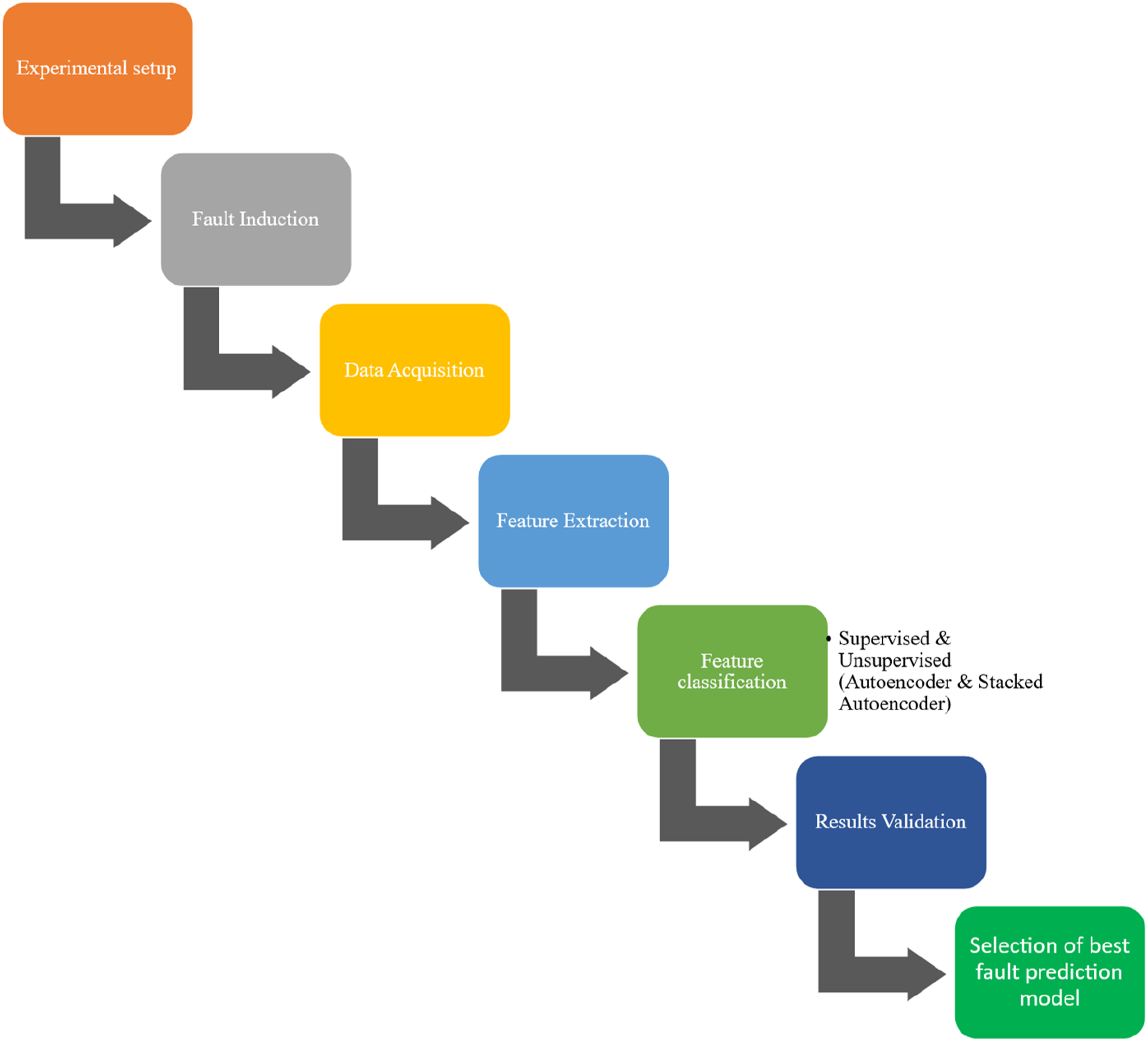

Experimental setup

Noticeable changes in the system output, efficiency loss, temperature, aggressive vibrations, sounds, etc., always detect the fault of a mechanical system. One of the primary and quantifiable parameters must be chosen for adequate identification. The parameters that have been selected are vibration, sound, and AE signals. These signals can be acquired from the gearbox with the help of advanced data science technologies.⁴¹ The experimental setup consists of the following types of sensors and data acquisition system.

• 3 – Phase induction motor.

• 4 – speed synchronous gearbox.

• Eddy current dynamometer

• Piezoelectric triaxial accelerometer.

• Physical acoustics AE sensor.

• Physical acoustics data acquisition system.

• 40PH free-field array microphone.

• Vib pilot 8-channel data acquisition system.

The experimental setup consists of three 3-phase induction motors, a 4-speed gearbox, and a dynamometer. The induction motor acts as the power source to replace a combustion vehicle’s engine, and the motor’s speed is controlled by delta drive. The output of the gearbox is coupled with an eddy current dynamometer. A vehicle’s dynamic working conditions are simulated with a dynamometer’s help to induce load onto the gearbox. The motor and dynamometer are coupled to the gearbox with a flexible coupling and are fixed rigidly to a stationary table, as shown in Figure 2. The operating speed of the gearbox was maintained between 0 and 1440 rpm, but for safety concerns, the maximum speed of the motor was held at 1000 rpm. The following faults were induced to gear³ and bearing⁷ with reference to existing literature. The gear teeth was induced with adhesion type wear by machine grinding operation, and a bearing crack was introduced on the outer race of a bearing using Electric Discharge Machining (EDM).

Figure 2.

Experimental setup.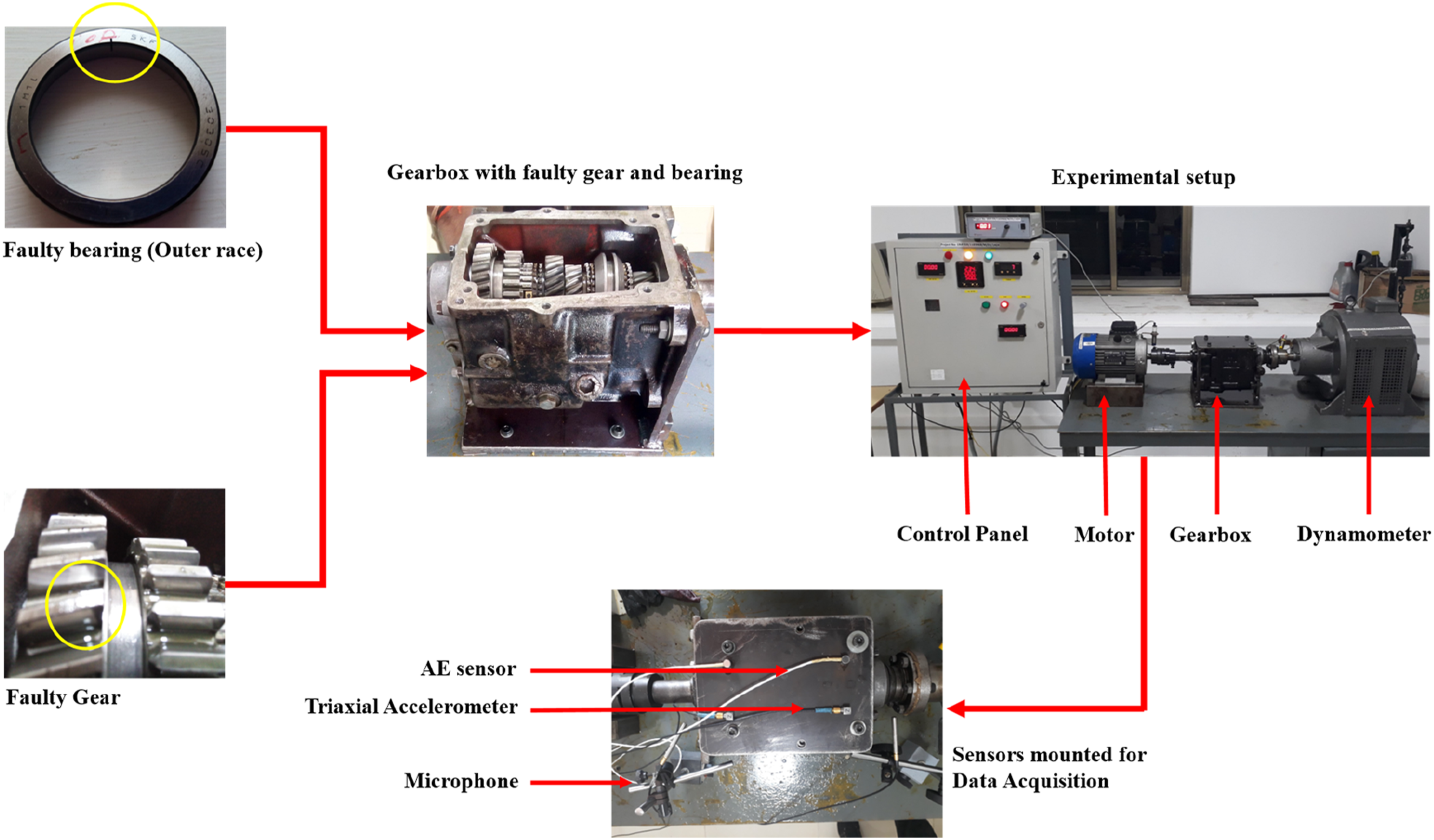

A triaxial accelerometer and AE sensors were rigidly mounted on the top surface of the gearbox above the bearing housing, and a 40PH free-field array microphone was fixed near the bearing housing of the gearbox. The accelerometer and microphone sensors are connected to an 8-channel Data Acquisition System (DAQ) to acquire the vibration and sound signals. The AE sensors are connected to the acoustic data acquisition system to receive respective AE signals from the gearbox.

Experimental procedure

The data has been acquired from the gearbox and categorized under four combinations of gear and bearing fault classes: Good Gear - Good Bearing (D1); Good Gear – Falt Bearing (D2); Fault Gear - Good Bearing (D3); and Fault Gear - Fault Bearing (D4). The experimental setup was designed to operate under selected load (0 Nm, 5 Nm, and 10 Nm) and motor speed (500 rpm, 750 rpm, and 1000 rpm) conditions with gear speeds (1st, 2nd, 3rd, and 4th) leading (4 gear speeds × 4 fault classes × 3 motor speeds × 3 loads) to a total of 144 test conditions, represented in Table 1. Initially, the gearbox was operated under 1_D1_500_0, schematically illustrating 1^st gear with good gear and good bearing fault condition (D1) under the motor speed of 500 rpm with no resisting torque (0 Nm) by the dynamometer. The gearbox was left to run for a specific time for each test condition to maintain consistency while acquiring the data. Then, the data was acquired for 200 s at a sampling rate of 8192 samples per second using the DAQ systems. Similarly, the data has been acquired under 144 test conditions for all three signals, respectively.

Table 1.

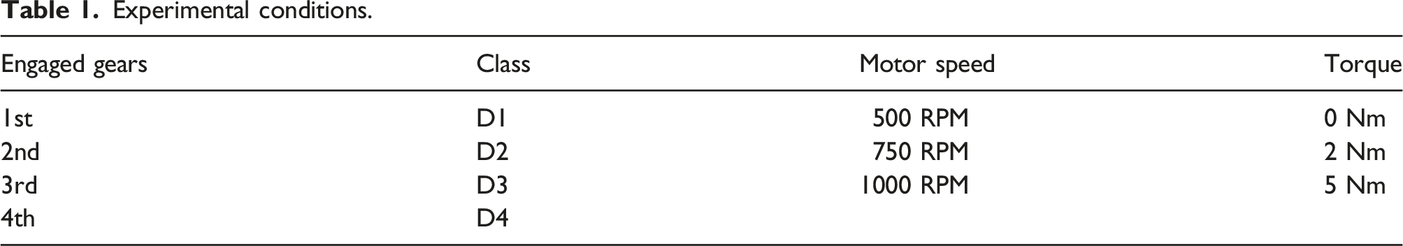
Experimental conditions.

Engaged gears	Class	Motor speed	Torque
1st	D1	500 RPM	0 Nm
2nd	D2	750 RPM	2 Nm
3rd	D3	1000 RPM	5 Nm
4th	D4

The real-time data acquired from the gearbox contains hidden information about the gearbox’s condition, which has to be extracted by the feature extraction method as they best differentiate the condition indicators in the data and reduce the probability of misclassification of faults. Using decision tree algorithm, the extracted feature were selected.³⁰ The statistical features such as mean, median, mode, Kurtosis, skewness, standard deviation, crest factor, RMS, Krms, and variance and acoustic features such as amplitude, count, RMS, frequency, and wavelength, are extracted from the acquired signals, as shown in the Tables 2 and 3. The extracted data contain 100 data points for each statistical feature under simulated speed and load conditions (100 data points × 10 statistical features).

Table 2.

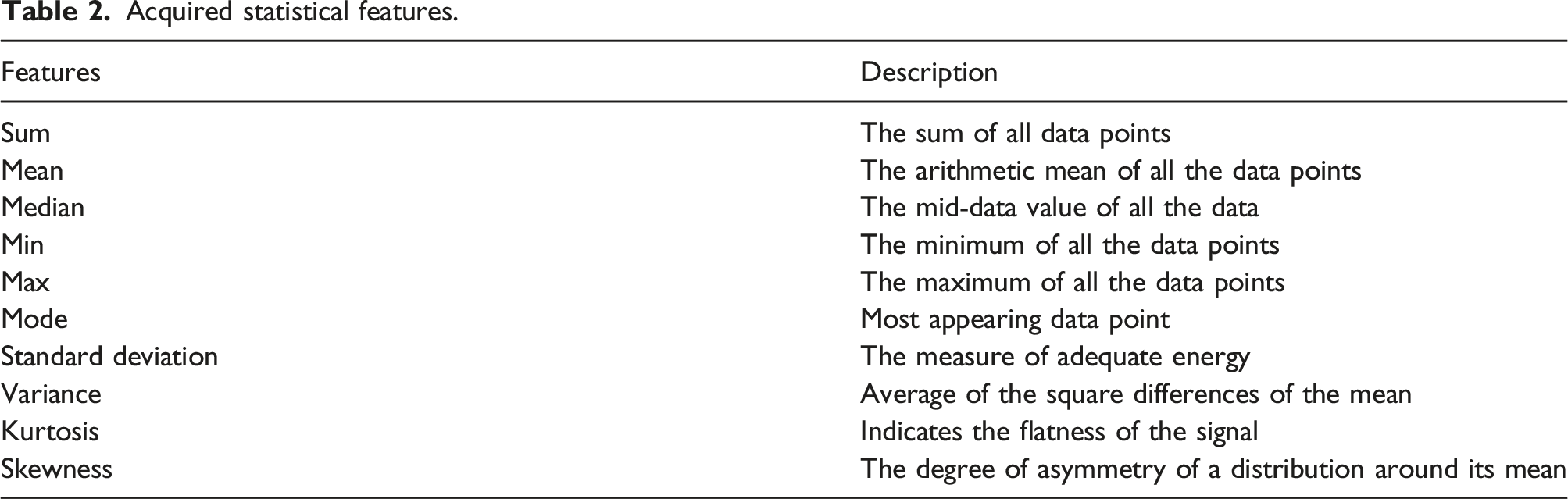
Acquired statistical features.

Features	Description
Sum	The sum of all data points
Mean	The arithmetic mean of all the data points
Median	The mid-data value of all the data
Min	The minimum of all the data points
Max	The maximum of all the data points
Mode	Most appearing data point
Standard deviation	The measure of adequate energy
Variance	Average of the square differences of the mean
Kurtosis	Indicates the flatness of the signal
Skewness	The degree of asymmetry of a distribution around its mean

Table 3.

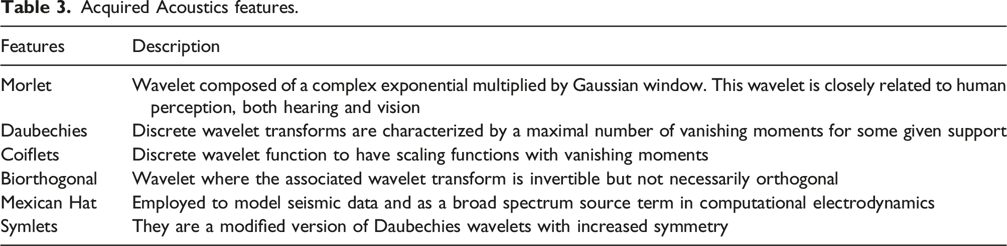
Acquired Acoustics features.

Features	Description
Morlet	Wavelet composed of a complex exponential multiplied by Gaussian window. This wavelet is closely related to human perception, both hearing and vision
Daubechies	Discrete wavelet transforms are characterized by a maximal number of vanishing moments for some given support
Coiflets	Discrete wavelet function to have scaling functions with vanishing moments
Biorthogonal	Wavelet where the associated wavelet transform is invertible but not necessarily orthogonal
Mexican Hat	Employed to model seismic data and as a broad spectrum source term in computational electrodynamics
Symlets	They are a modified version of Daubechies wavelets with increased symmetry

The evaluation of the algorithm had to be achieved by combining data points under three combinations, namely, condition 1, condition 2, and condition 3. Condition 1 represents individual data containing 12,000 data points (100 data points × 10 Features × 3 loads × 4 fault classes) for each motor and gears speeds; condition 2 represents speed-wise representation containing 36,000 data points (12,000 data points × 3 Motor Speeds) for each gear speeds and condition 3 represents gear-wise data containing 48,000 data points (12,000 data points × 4 gear speeds) for each motor speed, shown in Table 4.

Table 4.

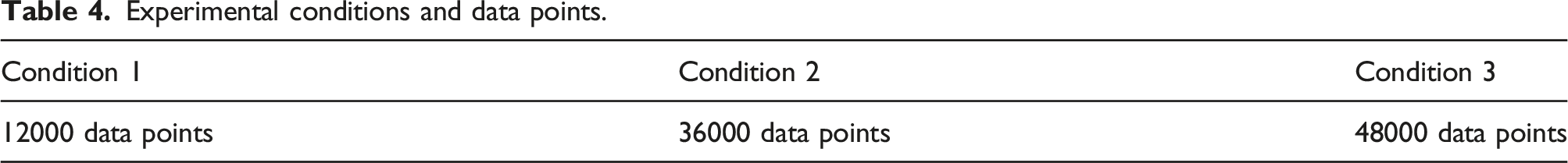
Experimental conditions and data points.

Condition 1	Condition 2	Condition 3
12000 data points	36000 data points	48000 data points

Deep learning approach

The neural networks are built with several layers of artificial neurons, which are the data processing units of the algorithms. These artificial neurons perform similar tasks to biological neurons and are interconnected to the nearby layers of neurons. The neural network mimics the neural system of a human brain, where the networks analyze the input data. However, high-dimensional input data require advanced neural network techniques such as deep learning with multiple layers of neural network that can perform high-dimensional recognition of data samples with a complex neural structure.⁴² Unlike traditional machine learning algorithms, which need the user to identify the features, deep learning algorithms identify the features without user intervention.⁴³ Deep learning models excel in gearbox fault detection by automatically learning complex patterns, handling non-linearities, and adapting to variable conditions, offering robust and efficient real-time monitoring compared to traditional methods. The solutions of the deep learning algorithms are end-to-end analysis, while the traditional algorithms depend on a series of conclusions. The deep learning algorithms utilize the maximum of any unstructured data by eliminating separate feature engineering. Even without data labeling, the algorithms produce accurate classification with high-dimension data.⁴⁴ The deep learning algorithms such as Supervised Deep Feed Forward Neural Network, Unsupervised Deep Feed Forward Neural Network, auto-encoder, and Stacked auto-encoder are proposed in this work, which is modeled to accommodate vibration, sound, and AE signals for improved fault classification.

Deep feed forward neural network

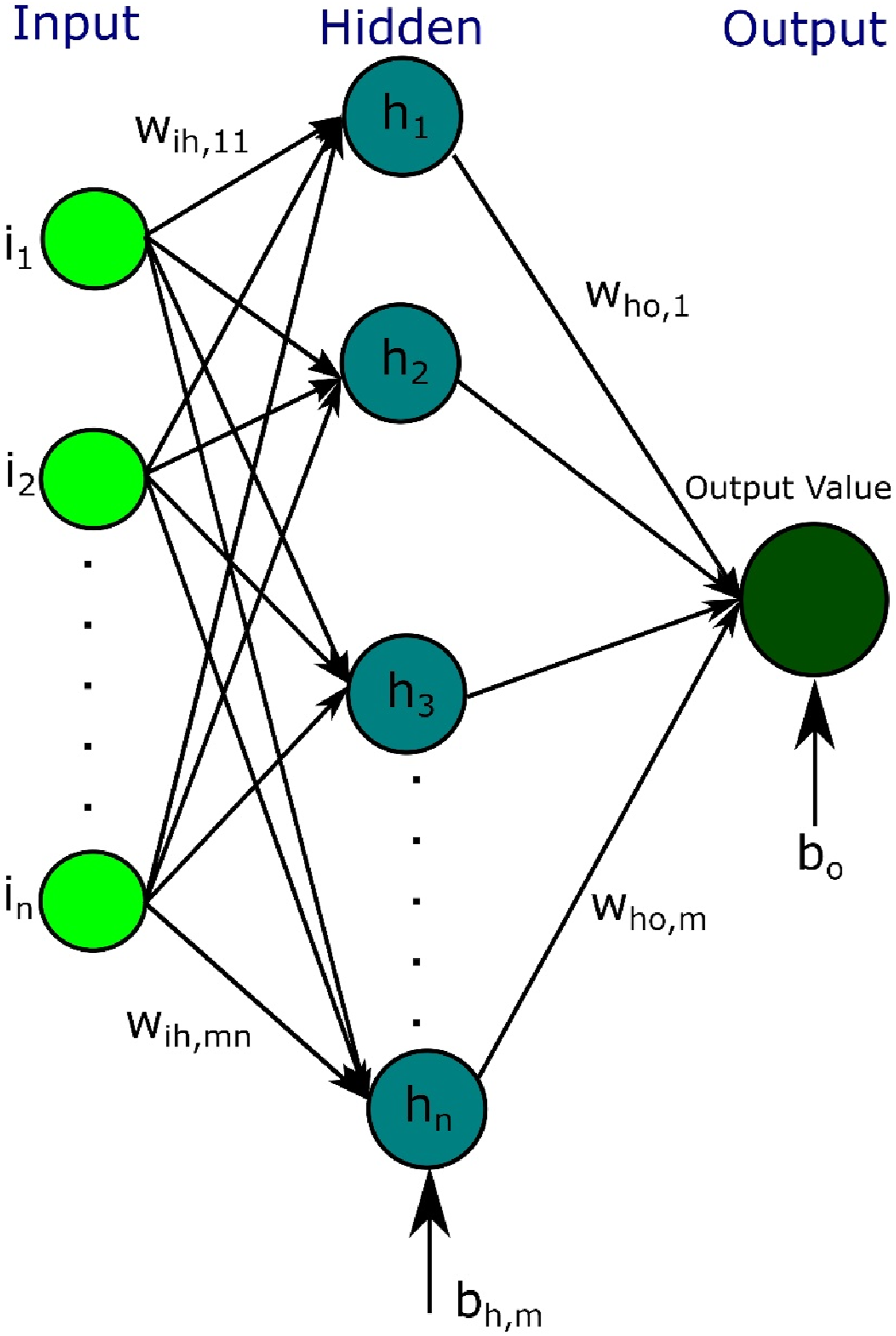
A Feed Forward Neural Network (FFNN) is a straightforward algorithm that utilizes the information in the input data.⁴⁵ It consists of input, hidden, and output layers of neurons where neurons of one layer are interconnected to neurons of the next layer, as shown in Figure 3.⁴⁶ The number of neurons in the input layer is equal to the number of input features, and the input layer processes the data, passes it to the next layer of the algorithm, and eventually reaches the output layer. The number of output layers is equal to the number of feature classes, and each neuron consists of an activation function and a set of hyper-parameters, such as weight and bias values that need to be defined and tuned for analyzing the data upon sequential training and testing as shown in equation (1). These hyper-parameters help in understanding the input data for fault diagnosis

F (x) = a (W^{T} x + b)

(1)

Figure 3.

Feed forward neural network.⁴⁶

The results of the activation function can be continuous or discrete, so a bias variable is used to categorize the output into classes, either true or false. This method is utilized by iterative training and testing to define the hyper-parameters. The reliable activation functions that produce higher classification accuracy are as follows.

SIGMOID function

The sigmoid function is a logistic function that results in a continuously S-shaped curve. The sigmoid curve runs between 0 and 1. This function can be utilized by biasing the results either 1 or 0, making the output binary. Equation (2) represents the function of the sigmoid function

a (x) = 1 / (1 + e^{- 6})

(2)

RELU function

The RELU function is the rectified linear unit function, which outputs 1 for positive and 0 for negative values. The function has no complex mathematics and so takes less time for computation. The function is sparsely activated, which has more predictability and less chance of over-fitting or noise, as shown in equation (3)

a (x) = \max (0, x)

(3)

Tanh function

The tanh function, as shown in equation (4), is a non-linear function that results in a continuous curve falling between the range [−1 1]. The curve is saturated before −1 and after 1, making it suitable for classification. The gradient is much stronger when compared to sigmoid but also has a vanishing gradient problem

a (x) = \frac{e^{x} - e^{- x}}{e^{x} - e^{- x}}

(4)

A deep Feed Forward Neural Network (DFFNN) algorithm has more than one hidden layer. The algorithm works on the same concept but involves complex relationships within and between the layers of neurons. This enables the use of low-dimensional data for improved daily detection.⁴⁷

These algorithms can be either supervised or unsupervised. The supervised DFFNN uses the known data to train and update the hyper-parameters, which involve user intervention in the learning process as the data has to be predefined for learning. The predefined data consists of data samples mapped to their respective condition classes. In contrast, the unsupervised DFFNN learns upon the unknown data where the data points are unmapped. This self-learning algorithm can be utilized in various automation processes by reducing its neural complexities. The base plot of this algorithm was improvised to many different algorithms by employing various functions, optimizer, stack flow, etc.⁴⁸

Architecture of DFFNN

The DFFNN is tested and compared in two forms: Supervised and Unsupervised DFFNN. The supervised DFFNN is programmed with more than one layer, where each layer consists of two parts: Activation and Dropout. A scheduled learning rate and a compatible optimizer can be employed in experimentation to increase classification accuracy. The supervised DFFNN experiments with various library functions to perfect the algorithm to maximize the classification accuracy as much as possible.

Dense layer

The neural networks can represent any complex data that has more non-linearity. Since the complex structure of the algorithm can reduce the efficiency of the training process with overlapping and vanishing gradients, the dense layer was introduced to gain a performance boost. The dense layer is a deeply connected layer with an element-wise activation function. The dense block connects every layer of the algorithm, reducing the vanishing gradient issue and the features being reused and reducing the number of parameters.⁴⁹ The number of neurons in the layer defines the shape of the output of the dense layer. The layers accept 2D input and give a 2D output. The dense layer supports a set of arguments used to enhance efficiency, including units, activation functions, initializers, and bias vectors.⁵⁰ The activation function selected for this project was “tanh” as it was experimented with to achieve higher accuracy for this data type. The tanh function is an asymptote that can be standardized using a bias vector.⁵¹ The final output layer is activated with the SoftMax function. Each dense block gave an output of 8 units as input to the dropout block.

Dropout block

The complex multilayer algorithm results in over-fitting data in the training process. The over-fitting phenomenon will reduce the efficiency of the learning process. It will result in lower classification accuracy and a higher training period, which can be avoided using a dropout block. The dropout block is a regularization method that reduces over-fitting by avoiding complex co-adaptations on training data. It drops out one unit of hidden and visible layers of a neural network, reducing the complexity of the neural network. This dropout also simulates sparse activation, enabling the network to learn in a sparse method like auto-encoders.⁵²

Auto-encoder and stacked auto-encoders

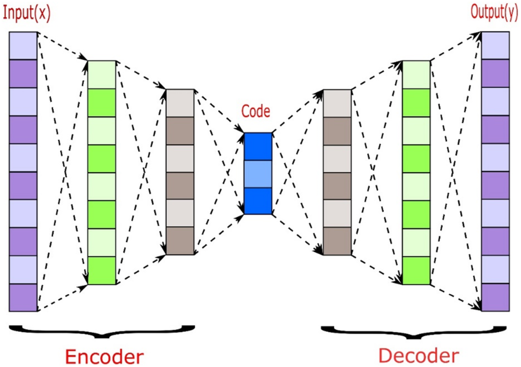
The different combinations and process flow of data have led to the development of many algorithms, one of them being auto-encoders. The auto-encoder algorithm is an unsupervised algorithm that receives the input data, encodes them into a compressed version, and decodes them to reconstruct the input, as represented in Figure 4.

Figure 4.

Auto-encoder.⁵³

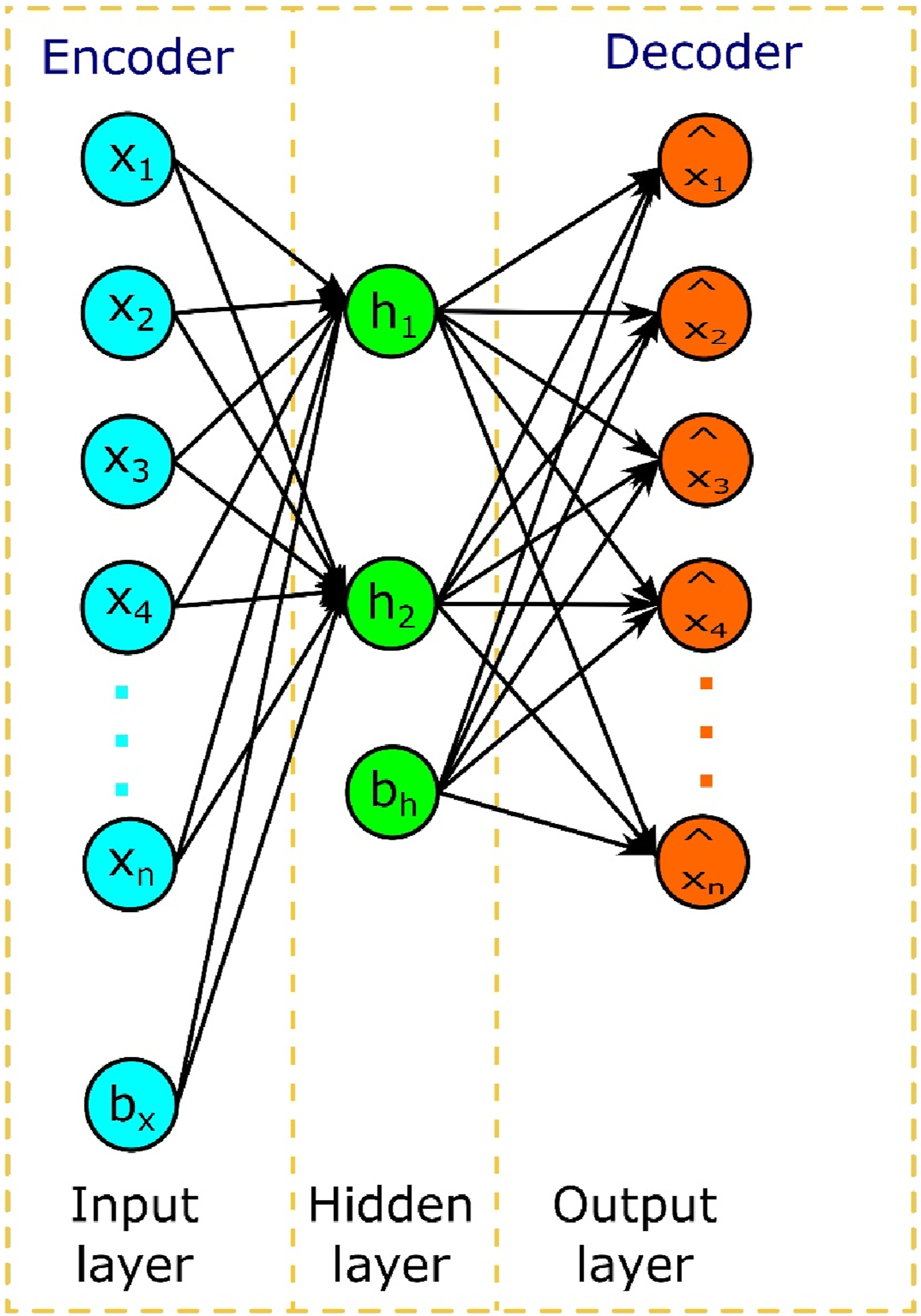
The auto-encoder is efficient when the regression of the output is nearly the same as the input. The auto-encoders are defined to recreate the information to understand the given data, hence better-updating hyper-parameters. The end-to-end structure of the algorithms with proper stacking is encoding and decoding layers, as shown in Figure 5,⁵⁴ which can produce better classification accuracy with high-dimensional data and is best suited for highly varying dynamic analysis of a mechanical system.

Figure 5.

Stacked auto-encoder.⁵⁴

Mathematically, the input vector is represented and mapped to hidden layers through a deterministic mapping $y = f (x)$ , parameterized as shown in equations (5)–(7)

x ϵ [0, 1] d

(5)

y ϵ [0, 1] d

(6)

⊝ = W, b

(7)

The auto-encoder can be represented in two parts: the encoder, defined as y = f(x), and the decoder, $z = g (y)$ . The value of z is almost equal to x. The input data is passed through the input layers to obtain the deterministic map y, as shown in equation (8)

y = f (x) = a (W T_{x} + b)

(8)

The “a” is an activation function, W is the weight matrix, and b is a bias variable. The encoder compresses the input data to a lower-level data known as the code. In contrast, the decoder consists of the output layers that are inversely mapped to obtain z, as shown in equation (9)

z = f (x) = a (W^{'} + b^{'})

(9)

where a is an activation function, W is the decoder weight matrix, and b is the decoder offset vector. The decoder reconstructs the code near its original dimension. In this process, the algorithm understands the trend of the data and updates its hyper-parameters under many iterations. The parametrizing variable is optimized to minimize the decoding error and is represented in equation (10)

\emptyset = \arg . \min \frac{1}{n} \sum_{i = 1}^{n} L (x^{i}, g_{\emptyset}, (f_{\emptyset} (x^{i})))

(10)

L is the loss function, and the x and z are reconstructed as vectors or probabilities. The loss can further be decreased by stacking the auto-encoder. The stacked auto-encoder (SAE) is a deep learning algorithm that uses stacked layers of the auto-encoder. This system involves layer-wise training where the output of one auto-encoder is the input to the next autoencoder. The algorithm efficiently learns the data pattern and can further precisely tune the parameter, leading to better classification.⁵⁵

Among these highlighted activation functions, the tanh and sigmoid are similar, but the tanh is bounded between (−1, 1), whereas the sigmoid is (0, 1), preventing more significant gradient values. The tanh function is centered around the value 0, whereas the sigmoid is 0.5 and so making. Moreover, since the tanh derivative is 1, the W and b in equation (1) are more expensive and quickly updated by the next layer. Hence, tanh is chosen as the primary activation function in the algorithms. The DFFNN is enabled only with the tanh function in every neuron layer. The auto-encoder is also enabled with the tanh function for activation for both encoding and decoding operations, as mentioned in equations (8) and (9). As mentioned above, these algorithms are tested and analyzed to give better results for the performance evaluation of a mechanical gearbox using the acquired data.

Evaluation of algorithm

The algorithm performance assessment was essential to optimize their ability to handle input data efficiently for enhanced fault classification in gearbox systems. The proposed machine learning algorithms will analyze the extracted statistical features for fault detection of the gearbox. The algorithms had to be evaluated under three evaluation conditions: individual data, gear-wise data, and speed-wise data, referred to as condition 1, condition 2, and condition 3, respectively. These conditions help analyze the working efficiency and complexity of the algorithms by which the algorithms can be optimized to use the given gearbox dataset. The hidden relation between the number of layers, steps per iteration, learning rate, weight decay, etc., can be analyzed and set to an optimum value.

The user-monitored fault classifier is the supervised DFFNN constructed with iterative updates of weight and bias matrices with the proper neural network of every neurons. The network is connected through 4 layers of neurons, including input and output layers. Every neuron of the layers is interconnected using ADAM optimizers and includes an L1-L2 regularizer. The RELU activation function assists the iterative updation of the hyper-parameters. The RELU function activates the required neuron during back-propagation. This helps in reducing the computation memory needed and speeding up the process. The number of layers, learning rate, iterations, steps per iteration, regularization, and decay rate were experimented and optimized to accommodate the input data and utilize its maximum potential. The classification accuracy of the algorithm was higher under condition 3 (48,000 samples) than condition 2 (36,000 samples), followed by condition 1 (12,000 samples), as shown in Table 5.

Table 5.

Classification accuracy of supervised DFFNN.

	Speed (rpm)	Gear 1	Gear 2	Gear 3	Gear 4	Combined gear-wise data (36000 samples)				Combined speed-wise data (48000 samples) (rpm)
	Speed (rpm)	12000 samples per gear				Gear 1	Gear 2	Gear 3	Gear 4	500	750	1000
Vibration	500	92.63	93.13	93.36	93.28	93.31	93.48	93.55	93.71	94.76	95.48	96.33
	750	93.88	94.29	94.84	94.31
	1000	94.91	94.99	95.37	95.46
Sound	500	88.08	88	88.26	88.48	90.02	90.28	90.34	90.48	90.27	91.18	92.36
	750	89.56	89.26	89.84	89.65
	1000	90.16	90.24	90.15	90.29
AE	500	84.5	84.48	84.45	84.51	86.29	86.34	86.38	86.42	86.09	86.94	88.13
	750	85.62	85.56	85.73	85.79
	1000	86.89	86.51	86.64	86.87

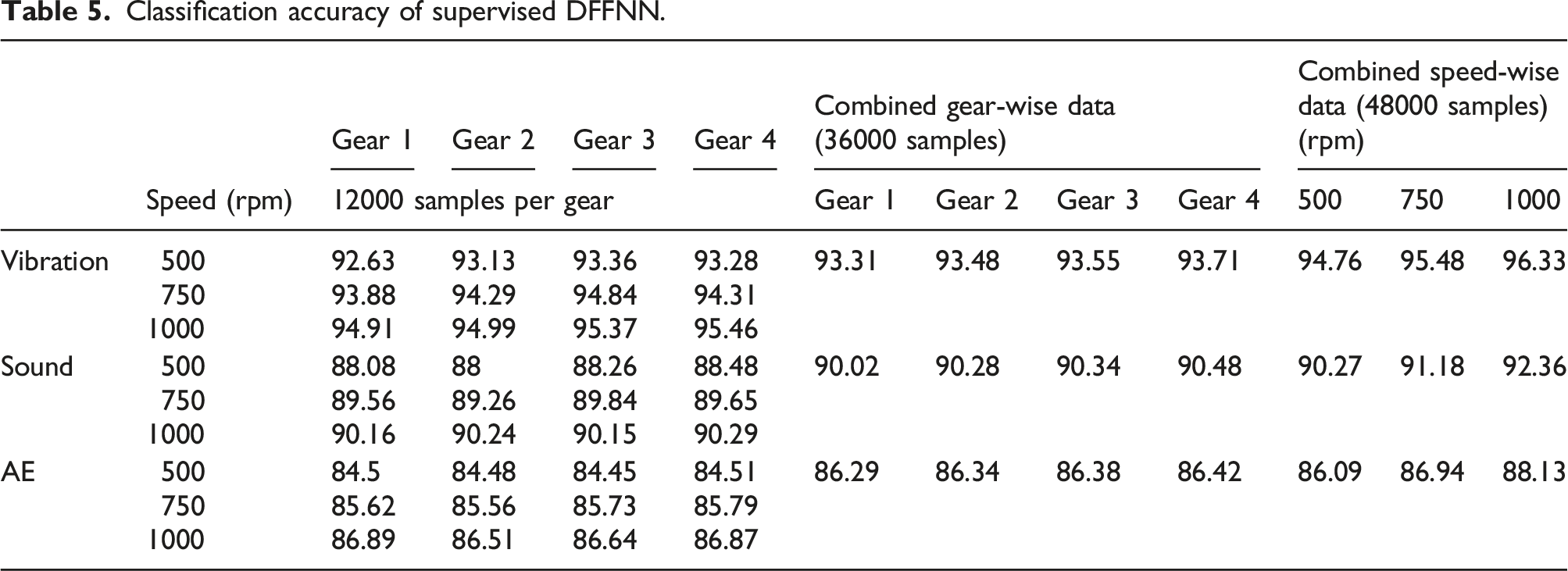
It was evident that the algorithm could precisely update with hyper-parameters with increased data samples under condition 3, providing more accuracy than SVM and Decision Tree algorithms.⁵⁶ The supervised DFFNN (S-DFFNN) algorithm also suffered high computation time under condition 3 and over-fitting of fault classes due to the increased complexity of the user-defined function in the algorithm. The automation of fault detection of any rotational mechanical system must employ a reduced complex neural network for faster classification involving available input data without human intervention.⁵⁷

Automating fault detection systems requires unsupervised neural networks to comprehend the hidden data pattern without human intervention. The algorithm was specifically optimized to improve the classification accuracy with sound and acoustic emission signals. An unsupervised DFFNN (US-DFFNN) is developed to enhance classification accuracy rather than a supervised neural network. The RELU function reached the early saturation state of updating the hyper-parameters and was replaced by the tanh function. It achieved lesser misclassification of faults and later saturation of hyper-parameters, as shown in Table 6. Although the input data has to be unlabeled, the condition column of the input data has been removed and shuffled before computation. The increased sample points in condition 3 revamped the algorithm to improve the classification accuracy by an average of 4.2 %. This drastically decreased the complexity of the network and, hence, the computation time.

Table 6.

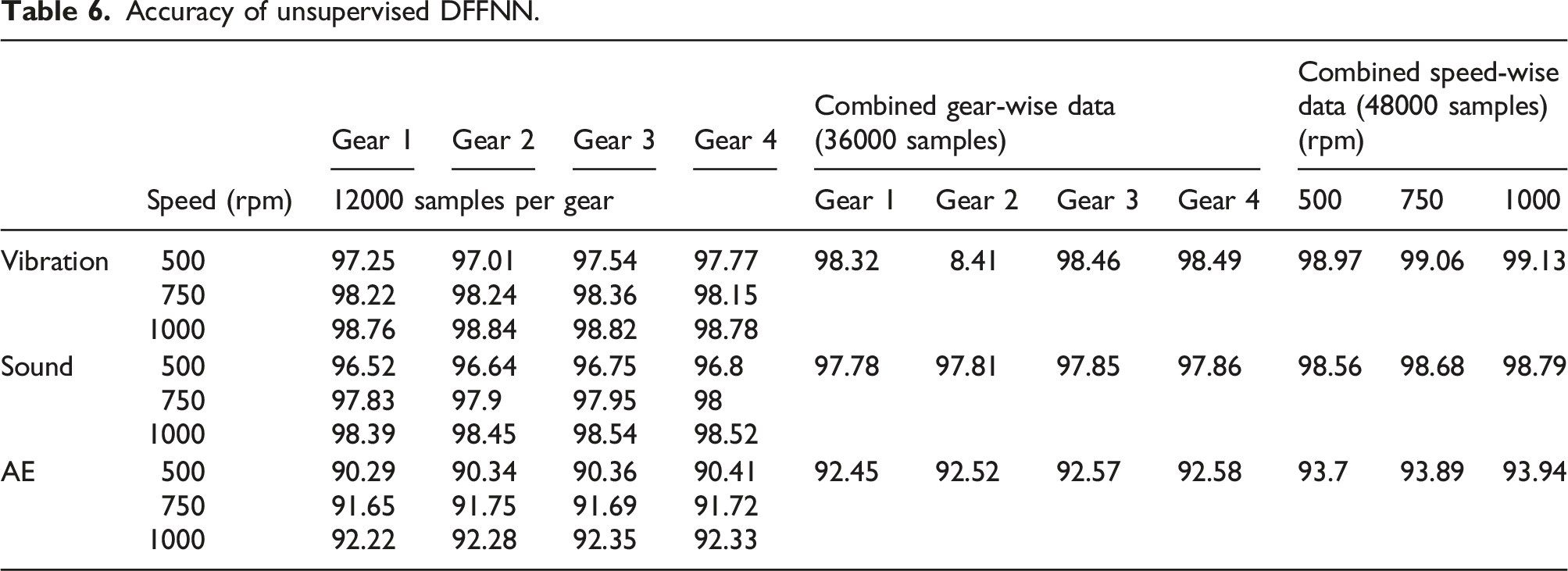
Accuracy of unsupervised DFFNN.

	Speed (rpm)	Gear 1	Gear 2	Gear 3	Gear 4	Combined gear-wise data (36000 samples)				Combined speed-wise data (48000 samples) (rpm)
	Speed (rpm)	12000 samples per gear				Gear 1	Gear 2	Gear 3	Gear 4	500	750	1000
Vibration	500	97.25	97.01	97.54	97.77	98.32	8.41	98.46	98.49	98.97	99.06	99.13
	750	98.22	98.24	98.36	98.15
	1000	98.76	98.84	98.82	98.78
Sound	500	96.52	96.64	96.75	96.8	97.78	97.81	97.85	97.86	98.56	98.68	98.79
	750	97.83	97.9	97.95	98
	1000	98.39	98.45	98.54	98.52
AE	500	90.29	90.34	90.36	90.41	92.45	92.52	92.57	92.58	93.7	93.89	93.94
	750	91.65	91.75	91.69	91.72
	1000	92.22	92.28	92.35	92.33

Further enhancement of the fault classification process can be done to decrease the misinterpretation of fault classes by introducing advanced machine learning techniques. Recent feature classification research employs auto-encoder algorithms for the rapid variety of high-dimensional signals. The auto-encoder algorithm is programmed with sequential encoding and decoding of input data to analyze the hidden gearbox condition indicators in the data, as discussed in Section 3.3. Like the unsupervised DFFNN, the condition labels in the input data are removed. The algorithms compress the input data into low-dimensional data and recreate the input data from the compressed data. Helpful information is acquired while reconstructing the input data. The encoding and decoding rates are independently controlled, so the algorithm is appropriately tuned to avoid over-fitting. The Adam optimizer with L1L2 regularizer is defined in the algorithm to reduce the computation time and improve the saturation state of the algorithm. The overall performance of the algorithm is enhanced by an average of 2.7 %, as represented in Table 7, further decreasing the computation time compared to the previous algorithm.

Table 7.

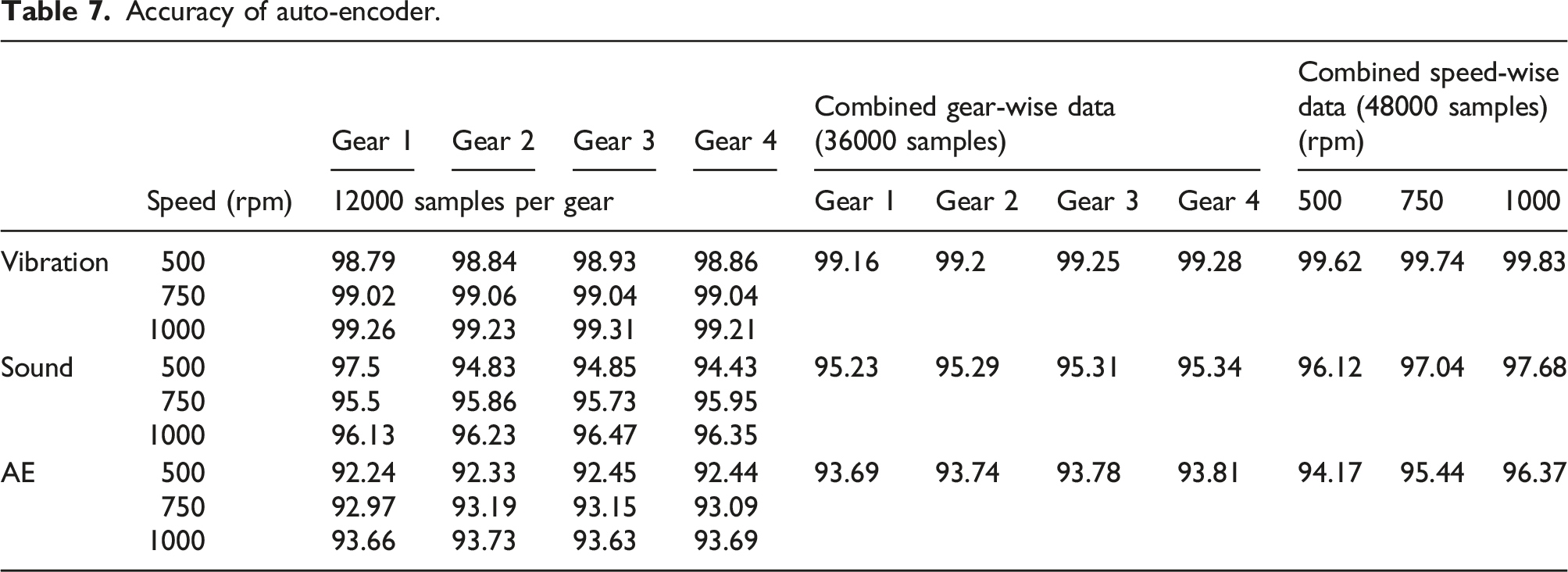
Accuracy of auto-encoder.

	Speed (rpm)	Gear 1	Gear 2	Gear 3	Gear 4	Combined gear-wise data (36000 samples)				Combined speed-wise data (48000 samples) (rpm)
	Speed (rpm)	12000 samples per gear				Gear 1	Gear 2	Gear 3	Gear 4	500	750	1000
Vibration	500	98.79	98.84	98.93	98.86	99.16	99.2	99.25	99.28	99.62	99.74	99.83
	750	99.02	99.06	99.04	99.04
	1000	99.26	99.23	99.31	99.21
Sound	500	97.5	94.83	94.85	94.43	95.23	95.29	95.31	95.34	96.12	97.04	97.68
	750	95.5	95.86	95.73	95.95
	1000	96.13	96.23	96.47	96.35
AE	500	92.24	92.33	92.45	92.44	93.69	93.74	93.78	93.81	94.17	95.44	96.37
	750	92.97	93.19	93.15	93.09
	1000	93.66	93.73	93.63	93.69

The automation of the fault detection system will be more responsive to fault detection with reduced computation time so that the auto-encoder can be stacked, moving the saturation point of the algorithm even further, as shown in Table 8. The decoding and encoding layers are increased by two, respectively, and inherit the same optimizer and regularizer. Although the algorithm’s complexity is increased by stacking the auto-encoder layers, the misclassification of the data was decreased, and the overall improvement of 0.2–0.8 % is achieved with half the computation time of the unstacked auto-encoder. The stacked auto-encoder extracted the best condition indicators in the vibration, sound, and AE signal data, making it suitable for an automated fault detection system.

Table 8.

Accuracy of stacked auto-encoder.

	Speed (rpm)	Gear 1	Gear 2	Gear 3	Gear 4	Combined gear-wise data (36000 samples)				Combined speed-wise data (48000 samples) (rpm)
	Speed (rpm)	12000 samples per gear				Gear 1	Gear 2	Gear 3	Gear 4	500	750	1000
Vibration	500	99.26	99.3	99.3	99.31	99.84	99.89	99.91	99.97	99.84	100	100
	750	99.62	99.69	99.71	99.75
	1000	99.89	99.91	99.98	100
Sound	500	95.75	95.56	95.74	95.76	96.65	96.72	96.69	96.71	96.98	97.81	98.42
	750	96.62	96.67	96.72	96.74
	1000	97.26	97.48	97.57	97.55
AE	500	93.56	93.79	93.84	93.86	94.6	94.73	94.89	95.03	95.7	96.63	97.11
	750	94.41	94.51	94.59	94.67
	1000	95.27	95.24	95.28	95.37

Results and discussions

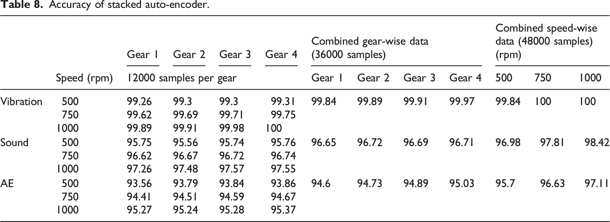
Based on the evaluation, the vibration signals perform best, resulting in higher classification accuracy. Figure 6(a) and (b) represents the average accuracy and time of the proposed algorithms using vibration signals. It is clear from the table that the accuracy of the algorithms increases with the number of data points in the vibration signals. The SAE algorithm produces the highest average accuracy of 99.95 % speed-wise combined. The computation time taken was 253 s for 250 iterations. The SAE is capable of achieving 100 % accuracy with high-dimensional data. The increase in the number of data points achieved better training results in higher accuracy when compared with individual and gear-wise combined data. This could be attributed to the non-linear transformations, data representation, deep architecture, adaptability to data size, regularization, and effective optimization.⁵⁸

Figure 6.

Accuracy using vibration signal. Here, (a) compares different classifier and their accuracy, (b) compares different classifier and their compilation time for vibration signal.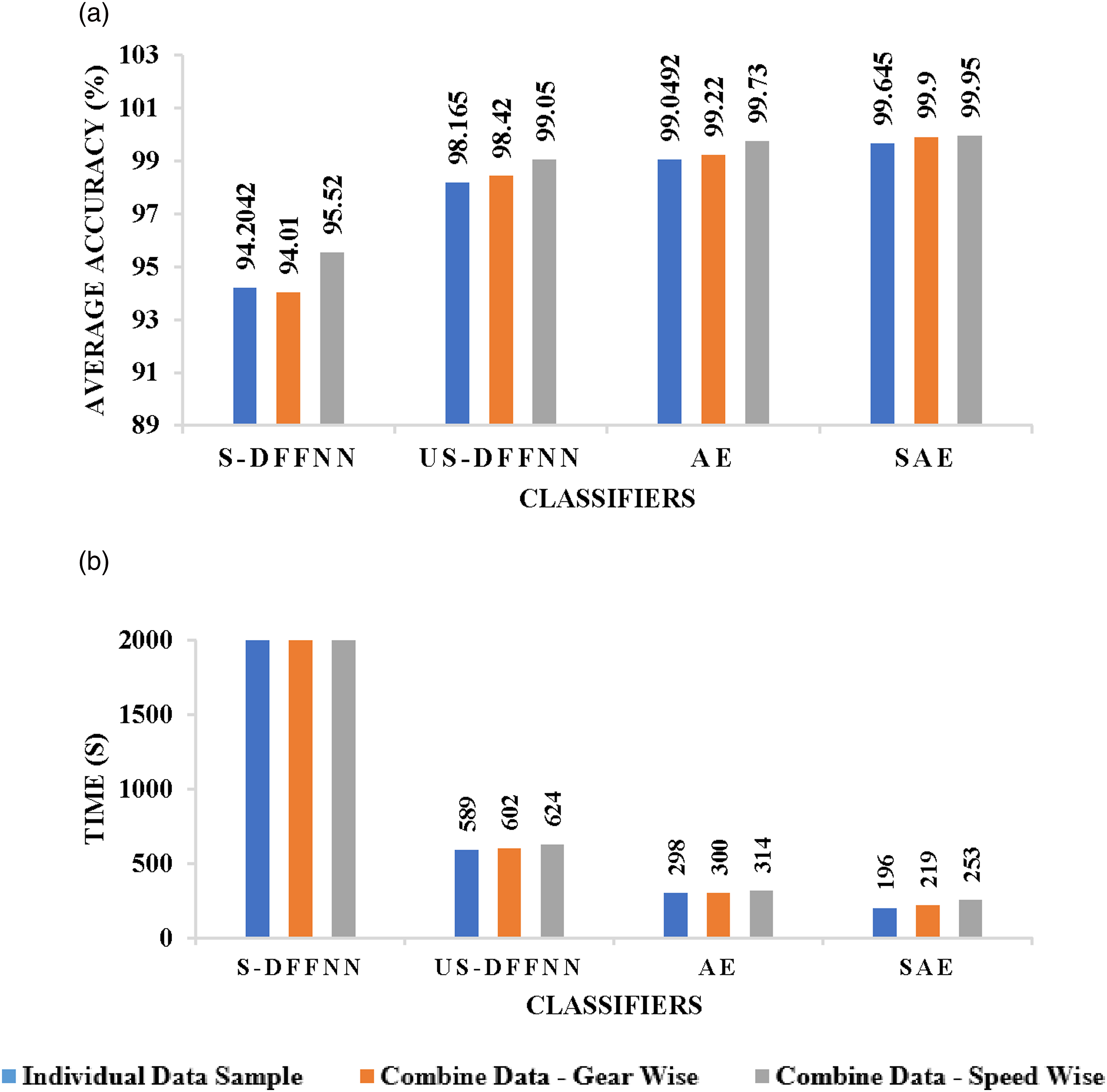

The sound signal data were not best explored as much as the vibration signal in previous research.^27,59 This work was primarily focused on optimizing the algorithms to achieve the highest classification accuracy with sound and AE signals. The average accuracy and time of the algorithms using sound signals is shown in Figure 7(a) and (b). Despite the stacked auto-encoder being the most robust classification algorithm, it can be depicted that the unsupervised DFFNN achieves the highest classification accuracy of 98.68 % with combined sound signal data. This is due to the coding and decoding process of the SAE algorithm, where the algorithm loses the information in the sound signal during the decoding process, resulting in slightly lesser accuracy than the unsupervised DFFNN. However, the unsupervised DFFNN requires a computation time of 600 s, while the SAE takes 262 s under 250 iterations with combined speed-wise data.

Figure 7.

Accuracy using sound signal. Here, (a) compares different classifier and their accuracy, (b) compares different classifier and their compilation time for sound signal.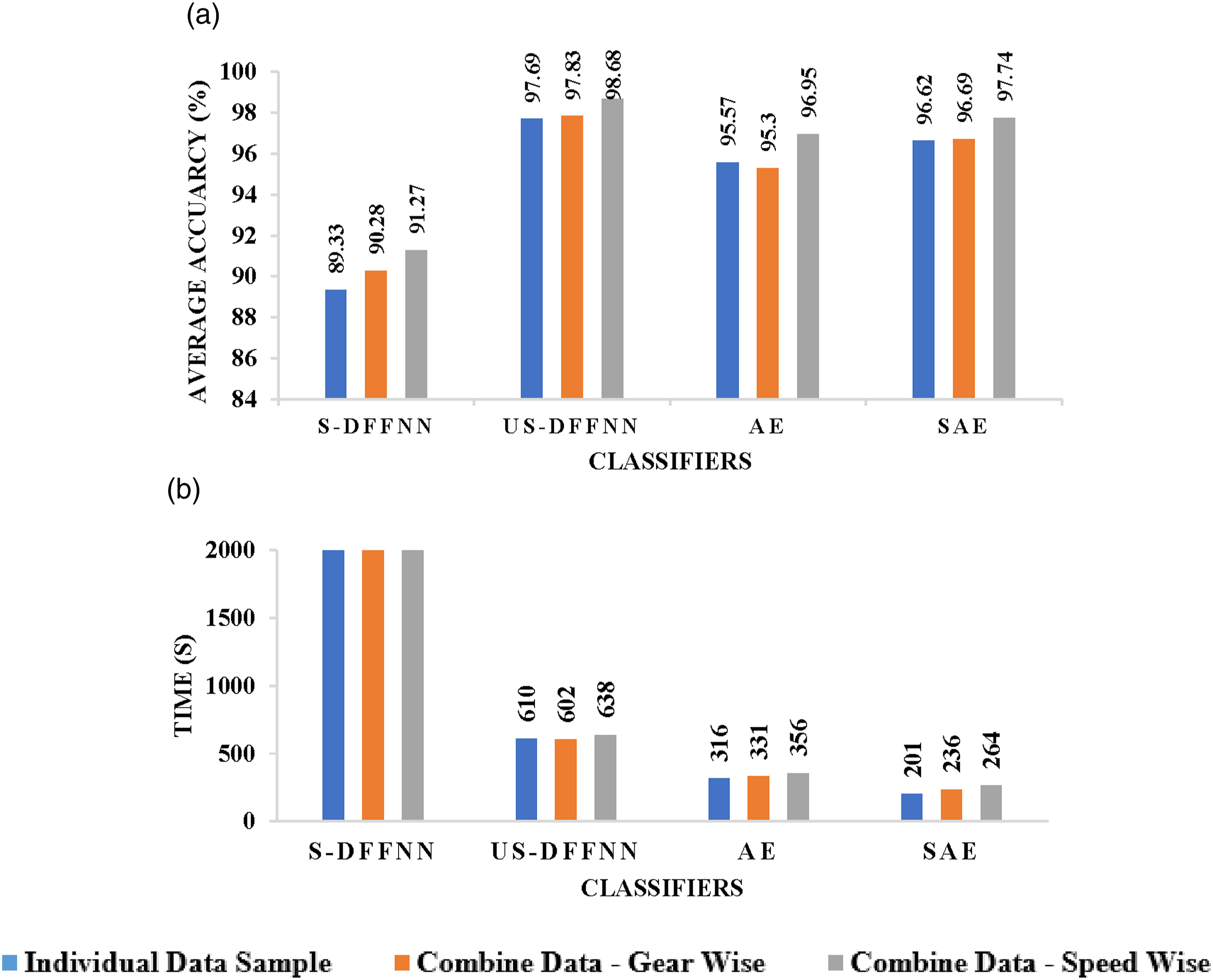

The difference in performance between the unsupervised DFFNN and the SAE when classifying sound signal data can be explained by the trade-off between feature representation and information loss during decoding. The DFFNN excels in feature learning and representation but requires more computation time. In contrast, while achieving high accuracy, the SAE may lose some information during the encoding and decoding process but does so with greater computational efficiency. The choice between these models depends on the application’s specific requirements, including the balance between accuracy and computational resources.

The AE features are directly acquired from the AE-DAQ system, so the loss of information in the data is lesser due to the avoidance of the feature extraction technique. Though the supervised algorithms suffered over-fitting with AE signal data, the unsupervised algorithms were primarily built to reduce over-fitting by regularizing the input. Figure 8(a) and (b) illustrates the average accuracy and time of algorithms with AE signal data. It can be inferred that the SAE algorithm can effectively analyze the AE signal data and achieve an average classification accuracy of 96.48 % with speed-wise combined AE signal data. With a sample size of 48,000 sample points, the speed-wise combined data guides the algorithm to achieve the highest classification accuracy with 248 s of computation time under 250 iterations.

Figure 8.

Accuracy using AE signal. Here, (a) compares different classifier and their accuracy, (b) compares different classifier and their compilation time for AE signal.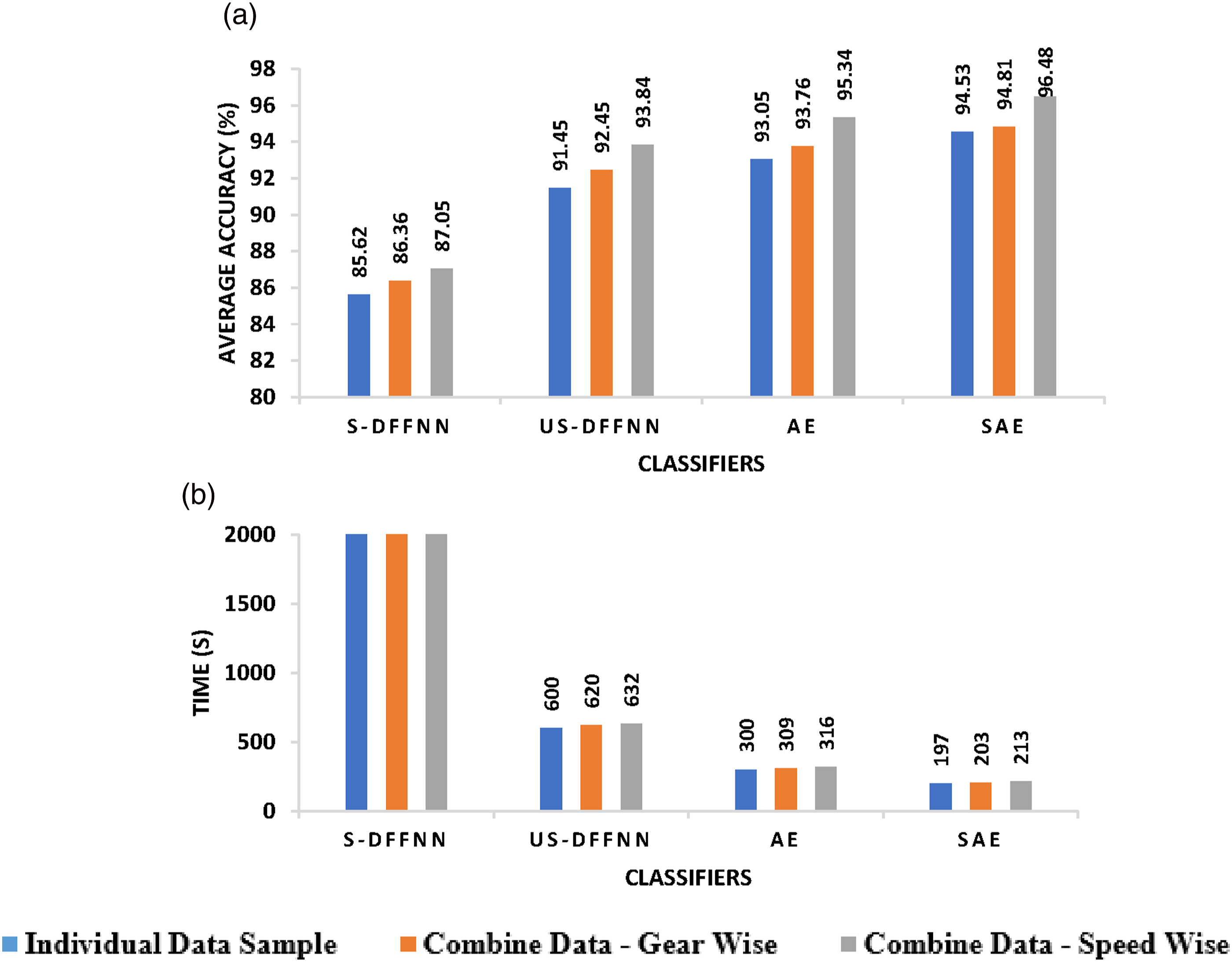

The success of the SAE algorithm when applied to AE signal data is consistent with the findings related to other signal types.^60–62 The key factors contributing to this success include direct data acquisition, the unsupervised learning advantage, regularization techniques, and access to a substantial volume of data, enabling the SAE to capture relevant information and achieve high classification accuracy effectively.⁶³ These factors, as outlined by Manikandan and Duraisamy,⁶⁴ indicate that SEA is a viable option for fault classification jobs over a wide range of signal types.

Based on the evaluation, it can be proved that the SAE provides higher classification accuracy using vibration and AE signals. The unsupervised DFFNN achieves slightly better classification accuracy than the SAE with sound signals because DFFNNs, with their more profound architecture, are better at capturing the intricacies of complex sound data. However, SAEs excel in computational efficiency due to their design, resulting in significantly shorter processing times. This trade-off is significant as it highlights the choice between higher accuracy (DFFNN) and faster real-time decision-making (SAE) in fault detection systems, with the preference depending on specific application requirements. Hence, the SAE algorithm can be used to automate fault diagnosis.

Conclusion

In this paper, the performance of the proposed deep algorithms for fault detection of the gearbox was optimized and evaluated. The vibration, sound, and acoustic emission signals are acquired from the gears and bearings of the gearbox. According to the literature and previous research, the properties of each signal data were studied to construct different neural networking algorithms. The following conclusions were drawn from this research.

• The supervised DFFNN can completely utilize the information in vibration signals. The sound and acoustic emission signals are not entirely utilized, resulting in less classification accuracy.

• The unsupervised algorithms are optimized and compared with the classification results using vibration signals to use reliable information on the acoustic emission and sound signals.

• The unsupervised neural networks provide an enhanced complex network that enables the network to train efficiently by regularizing the network and reducing the vanishing gradient phenomenon.

• The auto-encoder and stacked auto-encoder improve classification by utilizing the information in the acoustic emission signals, producing improved classification accuracy compared to supervised and unsupervised DFFNN.

• The stacked auto-encoder is a network with multiple layers of encoder and decoder with suitable optimizer and regularizer, reducing the computation time by 40 % and the memory consumption.

Even though the algorithms excel in their performance, they can be even more optimized to boost the performance, which is aimed to be continued with future research. With this excellent performance of the auto-encoder and SAE, which takes a lesser computation time while using vibration, sound, and acoustic emission signals, the algorithms can be utilized in an automated fault detection system. The real-time monitoring of any rotating mechanical system under dynamic conditions is possible and can be automated to preclude supervision.

Footnotes

Declaration of conflicting interests

The author(s) declared no potential conflicts of interest with respect to the research, authorship, and/or publication of this article.

Funding

The author(s) received no financial support for the research, authorship, and/or publication of this article.

ORCID iD

Solomon Jenoris Muthiya

References

Cano

Banham

, et al. Batteries and fuel cells for emerging electric vehicle markets. Nat Energy 2018; 3: 279–289.

Machado

Kollmeyer

Barroso

, et al. Multi-speed gearboxes for battery electric vehicles: current status and future trends. IEEE Open Journal of Vehicular Technology 2021; 2: 419–435.

Feng

, et al. A review of vibration-based gear wear monitoring and prediction techniques. Mech Syst Signal Process 2023; 182: 109605.

Zhou

Wenlei

. Vibration and noise radiation characteristics of gear transmission system. J Low Freq Noise Vib Act Control 2014; 33: 485–502.

Tama

Vania

Lee

, et al. Recent advances in the application of deep learning for fault diagnosis of rotating machinery using vibration signals. Artif Intell Rev 2023; 56: 4667–4709.

Hartono

Halim

Roberts

. Gear fault diagnosis using the general linear chirplet transform with vibration and acoustic measurements. J Low Freq Noise Vib Act Control 2019; 38: 36–52.

Wang

Tsui

K-L

Miao

. Prognostics and health management: a review of vibration based bearing and gear health indicators. IEEE Access 2018; 6: 665–676.

Jiang

, et al. Recent progress on decoupling diagnosis of hybrid failures in gear transmission systems using vibration sensor signal: a review. Measurement 2016; 90: 4–19.

Cubillo

Perinpanayagam

Esperon-Miguez

. A review of physics-based models in prognostics: application to gears and bearings of rotating machinery. Adv Mech Eng 2016; 8: 1687814016664660.

10.

Aherwar

. An investigation on gearbox fault detection using vibration analysis techniques: a review. Aust J Mech Eng 2012; 10: 169–183.

11.

Vishwakarma

Purohit

Harshlata

, et al. Vibration analysis & condition monitoring for rotating machines: a review. Mater Today Proc 2017; 4: 2659–2664.

12.

Wang

Han

Chu

, et al. Vibration based condition monitoring and fault diagnosis of wind turbine planetary gearbox: a review. Mech Syst Signal Process 2019; 126: 662–685.

13.

Zhou

Sun

Cao

. Vibration and noise characteristics of a gear reducer under different operation conditions. J Low Freq Noise Vib Act Control 2019; 38: 574–591.

14.

Zhang

Zhou

Wang

, et al. State of the art on vibration signal processing towards data-driven gear fault diagnosis. IET Collaborative Intelligent Manufacturing 2022; 4: 249–266.

15.

Raghav

Sharma

. A review on fault diagnosis and condition monitoring of gearboxes by using AE technique. Arch Comput Methods Eng 2021; 28: 2845–2859.

16.

Thangamuthu

Madheswaran

. The process parameter optimization for grey cast iron in turning process using response surface methodology. IJMPERD 2019; 9: 997–1006.

17.

Delvecchio

Bonfiglio

Pompoli

. Vibro-acoustic condition monitoring of Internal Combustion Engines: a critical review of existing techniques. Mech Syst Signal Process 2018; 99: 661–683.

18.

Saimurugan

Nithesh

. Intelligent Fault diagnosis model for rotating machinery based on fusion of sound signals. Int J Prognostics Health Manag 2016; 7. Epub ahead of print 2016. DOI: 10.36001/ijphm.2016.v7i2.2366

19.

Praveenkumar

Saimurugan

Ramachandran

. Comparison of vibration, sound and motor current signature analysis for detection of gear box faults. Int J Prognostics Health Manag 2017; 8: Epub ahead of print 2017. DOI: 10.36001/ijphm.2017.v8i2.2642

20.

Hang

Chen

, et al. An intelligent platform for ultrasound diagnosis of thyroid nodules. Sci Rep 2020; 10: 13223.

21.

Behnia

Chai

Shiotani

. Advanced structural health monitoring of concrete structures with the aid of acoustic emission. Construct Build Mater 2014; 65: 282–302.

22.

Caesarendra

Kosasih

Tieu

, et al. Acoustic emission-based condition monitoring methods: review and application for low speed slew bearing. Mech Syst Signal Process 2016; 72–73: 134–159.

23.

Ahn

Kim

Choi

. Artificial intelligence-based machine learning considering flow and temperature of the pipeline for leak early detection using acoustic emission. Eng Fract Mech 2019; 210: 381–392.

24.

Hou

Luo

, et al. Comparative study on the use of acoustic emission and vibration analyses for the bearing fault diagnosis of high-speed trains. Struct Health Monit 2022; 21: 1518–1540.

25.

Van Hecke

Yoon

. Low speed bearing fault diagnosis using acoustic emission sensors. Appl Acoust 2016; 105: 35–44.

26.

Praveenkumar

Sabhrish

Saimurugan

, et al. Pattern recognition based on-line vibration monitoring system for fault diagnosis of automobile gearbox. Measurement 2018; 114: 233–242.

27.

Kumar

Saimurugan

Haran

RBH

, et al. A multi-sensor information fusion for fault diagnosis of a gearbox utilizing discrete wavelet features. Meas Sci Technol 2019; 30: 085101.

28.

Jonak

. Early fault detection in gearboxes based on support vector machines and multilayer perceptron with a continuous wavelet transform. Appl Soft Comput 2015; 30: 636–641.

29.

Achirul Nanda

Boro Seminar

Nandika

, et al. A comparison study of kernel functions in the support vector machine and its application for termite detection. Information 2018; 9: 5.

30.

Saimurugan

Ramachandran

Sugumaran

, et al. Multi component fault diagnosis of rotational mechanical system based on decision tree and support vector machine. Expert Syst Appl 2011; 38: 3819–3826.

31.

Gunerkar

Jalan

Belgamwar

. Fault diagnosis of rolling element bearing based on artificial neural network. J Mech Sci Technol 2019; 33: 505–511.

32.

Martin-Diaz

Morinigo-Sotelo

Duque-Perez

, et al. An experimental comparative evaluation of machine learning techniques for motor fault diagnosis under various operating conditions. IEEE Trans Ind Appl 2018; 54: 2215–2224.

33.

Altobi

MAS

Bevan

Wallace

, et al. Fault diagnosis of a centrifugal pump using MLP-GABP and SVM with CWT. Engineering Science and Technology, an International Journal 2019; 22: 854–861.

34.

Grossberg

. Adaptive Resonance Theory: how a brain learns to consciously attend, learn, and recognize a changing world. Neural Network 2013; 37: 1–47.

35.

Wang

Qin

Wang

, et al. ReLTanh: an activation function with vanishing gradient resistance for SAE-based DNNs and its application to rotating machinery fault diagnosis. Neurocomputing 2019; 363: 88–98.

36.

Dias

Hadjileontiadou

Diniz

, et al. DeepLMS: a deep learning predictive model for supporting online learning in the Covid-19 era. Sci Rep 2020; 10: 19888.

37.

Abdul Gafoor

Sampathila

, et al. Deep learning model for detection of COVID-19 utilizing the chest X-ray images. Cogent Engineering 2022; 9: 2079221.

38.

Tang

Yuan

Zhu

. Deep learning-based intelligent fault diagnosis methods toward rotating machinery. IEEE Access 2020; 8: 9335–9346.

39.

Hoang

Kang

. A motor current signal-based bearing fault diagnosis using deep learning and information fusion. IEEE Trans Instrum Meas 2020; 69: 3325–3333.

40.

Mahmoud

Mohammed

. A survey on deep learning for time-series forecasting. In: Hassanien

Darwish

(eds). Machine Learning and Big Data Analytics Paradigms: Analysis, Applications and Challenges. Cham, Switzerland: Springer International Publishing, pp. 365–392.

41.

Dhar

Jayakumar

Lavanya

, et al. Techno-economic assessment of various motors for three-wheeler E-auto rickshaw: from Indian context. Mater Today Proc 2021; 45: 6572–6579.

42.

Wang

Fan

Wang

. Comparative analysis of image classification algorithms based on traditional machine learning and deep learning. Pattern Recogn Lett 2021; 141: 61–67.

43.

Sarker

. Machine learning: algorithms, real-world applications and research directions. SN COMPUT SCI 2021; 2: 160.

44.

Dong

Liu

. Feature engineering for machine learning and data analytics. Boca Raton, Florida: CRC Press, 2018.

45.

Hemeida

Hassan

Mohamed

A-AA

, et al. Nature-inspired algorithms for feed-forward neural network classifiers: a survey of one decade of research. Ain Shams Eng J 2020; 11: 659–675.

46.

Tripoppoom

Yong

, et al. Assisted history matching in shale gas well using multiple-proxy-based Markov chain Monte Carlo algorithm: the comparison of K-nearest neighbors and neural networks as proxy model. Fuel 2020; 262: 116563.

47.

Cuomo

Di Cola

Giampaolo

, et al. Scientific machine learning through physics–informed neural networks: where we are and what’s next. J Sci Comput 2022; 92: 88.

48.

Saha

Swetapadma

Mondal

. A brief review on artificial neural network: network structures and applications. In: 2023 9th international conference on advanced computing and communication systems, Coimbatore, India, 17–18 March 2023, pp. 1974–1979.

49.

Sze

Chen

Y-H

Yang

T-J

, et al. Efficient processing of deep neural networks: a tutorial and survey. Proc IEEE 2017; 105: 2295–2329.

50.

Anwar

Khan

Barnes

. A deep journey into super-resolution: a survey. ACM Comput Surv 2020; 53: :1–34.

51.

Rao

Liu

. Three-dimensional convolutional neural network (3D-CNN) for heterogeneous material homogenization. Comput Mater Sci 2020; 184: 109850.

52.

Guo

Liu

Oerlemans

, et al. Deep learning for visual understanding: a review. Neurocomputing 2016; 187: 27–48.

53.

Han

Wang

, et al. Application of deep canonically correlated sparse autoencoder for the classification of schizophrenia. Comput Methods Progr Biomed 2020; 183: 105073.

54.

Deepthi

Jereesh

. An ensemble approach for CircRNA-disease association prediction based on autoencoder and deep neural network. Gene 2020; 762: 145040.

55.

Soniya

Singh

. A review on advances in deep learning. In: 2015 IEEE workshop on computational intelligence: theories, applications and future directions. Asheville, North Carolina: WCI, 2015, pp. 1–6.

56.

Saimurugan

Praveenkumar

Krishnakumar

, et al. A study on the classification ability of decision tree and support vector machine in gearbox fault detection. Appl Mech Mater 2015; 813–814: 1058–1062.

57.

Duan

Xie

Wang

, et al. Deep learning enabled intelligent fault diagnosis: overview and applications. J Intell Fuzzy Syst 2018; 35: 5771–5784.

58.

Yang

Perdikaris

. Adversarial uncertainty quantification in physics-informed neural networks. J Comput Phys 2019; 394: 136–152.

59.

Praveenkumar

Saimurugan

Ramachandran

. Intelligent Fault diagnosis of synchromesh gearbox using fusion of vibration and acoustic emission signals for performance enhancement. Int J Prognostics Health Manag 2019; 10. Epub ahead of print 1 June 2019. DOI: 10.36001/ijphm.2019.v10i2.2738

60.

Zhang

Peng

, et al. A deep convolutional neural network with new training methods for bearing fault diagnosis under noisy environment and different working load. Mech Syst Signal Process 2018; 100: 439–453.

61.

Chen

Gryllias

. Intelligent Fault diagnosis for rotary machinery using transferable convolutional neural network. IEEE Trans Ind Inf 2020; 16: 339–349.

62.

Mian

Choudhary

Fatima

. A sensor fusion based approach for bearing fault diagnosis of rotating machine. Proc Inst Mech Eng O J Risk Reliab 2022; 236: 661–675.

63.

Ibrahim

Dong

Yang

. Machine learning driven smart electric power systems: current trends and new perspectives. Appl Energy 2020; 272: 115237.

64.

Manikandan

Duraivelu

. Fault diagnosis of various rotating equipment using machine learning approaches – a review. Proc IME E J Process Mech Eng 2021; 235: 629–642.

Performance evaluation of deep learning approaches for fault diagnosis of rotational mechanical systems using vibration,sound,and acoustic emission signals

Abstract

Keywords

Introduction

Experimental methodology

Experimental setup

Experimental procedure

Deep learning approach

Deep feed forward neural network

SIGMOID function

RELU function

Tanh function

Architecture of DFFNN

Dense layer

Dropout block

Auto-encoder and stacked auto-encoders

Evaluation of algorithm

Results and discussions

Conclusion

Footnotes

Declaration of conflicting interests

Funding

ORCID iD

References