Deconvolution beamforming based on a fast gradient algorithm for sound source localization

Abstract

Deconvolution beamforming has gotten increased attention as a way to improve the spatial resolution of delay-and-sum beamforming. It has the ability to decrease sidelobes and increase resolution. However, compared to conventional beamforming, the extra computation of the deconvolution method is a drawback. A more efficient approach is developed to improve the computing speed of the deconvolution method. Specifically, when tackling deconvolution problems, this method improves computational performance by combining Fourier operation with a fast gradient algorithm called the double momentum gradient algorithm. We compare the proposed method with two known effective deconvolution methods, namely the fast Fourier transform non-negative least squares algorithm and the fast iterative shrinkage threshold algorithm. The results of simulation and experiment reveal that the proposed method tends to give a better spatial resolution within a short computational time and is more suitable for engineering applications.

Introduction

Beamforming^1–3 is a signal processing technology based on the microphone array and can locate the sound source like a spatial filter. It was mostly employed in radar, communication, and sonar.^4–6 With the development of computer technology, beamforming, as a visualization tool of the spatial sound field, has been widely used in the field of sound source identification. ⁷ Through phase alignment and summation, conventional delay-and-sum beamforming obtains the relative amplitude and position map of a sound source in a particular measurement area.^8,9 However, due to the limitation of microphone array aperture and number, the accuracy of beamforming localization is limited, and the main lobe of the sound source localization image is large, so the localization is not accurate enough. Scholars begin to pay attention to and develop more clear sound source identification methods. Deconvolution beamforming attracts attention.^10–12 This method establishes a linear equation based on the relationship among the output results of conventional beamforming, array point-spread function, and sound source distribution, and obtains the real point source distribution in the beamforming map by solving the equation.

Some effective deconvolution methods were developed to improve the resolution of the beamforming map. Brooks et al. ¹³ proposed a deconvolution approach for the mapping of acoustic sources algorithm (DAMAS) based on Gaussian Saidel iteration. Dougherty et al. ¹⁴ proposed the CLEAN algorithm based on removing the contribution of the maximum sound source. In comparison to standard delay-and-sum beamforming, deconvolution methods typically require additional calculation work, which means that their calculation efficiency should be improved. Therefore, deconvolution beamforming based on the fast Fourier transform (FFT) is introduced. Dougherty et al. ¹⁵ proposed two extensions of DAMAS to reduce the computational effort. For the same purpose, Ehrenfried et al. proposed the FFT-based non-negative least squares (FFT-NNLS) algorithm, which combined the Fast Fourier Transform and non-negative least squares algorithm.^10,16 Lylloff proposed a fast iterative shrinkage-thresholding algorithm (FISTA) as an improvement of the FFT-NNLS algorithm.^17,18 It is more efficient among the existing deconvolution beamforming. Although the FFT-based algorithm can reduce computational complexity, its performance is significantly affected by the combined algorithm. Therefore, combining Fourier operation with a faster iterative algorithm can improve the computational efficiency of deconvolution method. Recently, scholars have concentrated on increasing the convergence speed of algorithms in engineering applications. Jihuan He proposed homotopy perturbation method (HPM) which is to combine the basic ideas of homotopy in topology and the classical perturbation techniques to continuously deform difficult problems into simple ones that are easily handled. It is one of the most powerful and efficient methods for a wide variety of problems and has been studied and developed by many scholars.^19–22 Khan proposed two improved algorithms based on Chun-Hui He’s iteration method, which can reduce the number of iterations and have important practical implications in different engineering fields.^23,24 In large-scale optimization problems, the first-order algorithm is an ideal choice because it is efficient and mildly sensitive to the dimension of the function.^25–27 In the field of signal processing, image processing, machine learning, big data analysis, or their cross-fields,^28–31 there are usually a lot of parameters to learn. It has great potential to improve the training efficiency by using the first-order algorithm in the process of model learning. Therefore, the first-order algorithm has become a research hotspot.^32,33

It is necessary to optimize the efficiency of the first-order algorithm before it is used for deconvolution beamforming. Optimizing this type of algorithm is challenging. Multiple relaxation stages are necessary in mathematics for optimization with an infinite-dimensional function constraint. Drori ³⁴ proposed a performance evaluator called performance estimation problem (PEP) for this issue by relaxing that infinite function restrictions. It uses the target value’s iteration boundary as the optimization objective, which allows for the optimization of the first-order method’s coefficients and the construction of a quicker first-order algorithm. Based on the PEP method, Kim and other researchers^35,36 have proposed a new optimization gradient algorithm, its coefficients can be achieved after optimization. It outperforms the commonly used Nesterov fast gradient technique in terms of convergence and computational efficiency.

On the basis of the above, we aim to develop and verify a new efficient deconvolution beamforming based on a fast gradient algorithm. Firstly, the objective equation of convolution beamforming is adjusted to the wave domain by Fourier transform. In the subsequent iterative process, the optimized algorithm with designed momentum terms is used to solve the modified equation effectively. The proposed method is called the fast Fourier transform double momentum gradient algorithm (FFT-DMG). The following is the outline: the second section discusses the process of optimizing the efficiency of the first-order algorithm, the third section discusses the improvement of deconvolution beamforming, the fourth and fifth sections conduct simulation and experimental analysis, and the sixth section concludes.

Optimization of algorithm efficiency

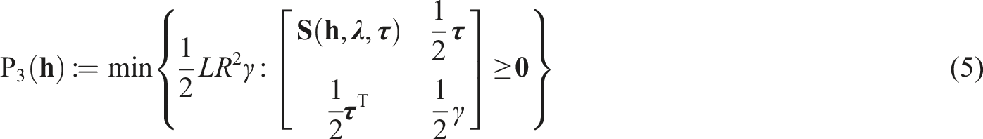
First-order techniques, such as the well-known Nesterov’s gradient method, are often employed to solve large-dimensional optimization problems, particularly in the domains of big data, machine learning, and signal processing. To maximize the performance of this kind of algorithm, or to build a new algorithm, a design-related cost function must be defined. It is vital to formalize the algorithm development process mathematically. Performance estimation problem is a novel approach to algorithm creation since it is capable of optimizing iterative parameters to create a faster method. The procedure finds a solution to the following problem

$\begin{array}{cc}{\mathrm{P}}_1\left(\mathbf{h}\right):=& \underset{\begin{array}{c}f\in {\mathcal{F}}_L\\ \Vert {\mathbf{x}}^{\left(0\right)}-{\mathbf{x}}^{*}\Vert \le R\end{array}}{\max }f\left({\mathbf{x}}^{\left(N\right)}\right)-f\left({\mathbf{x}}^{*}\right)\\ & \mathrm{s}.\mathrm{t}.\hspace{0.17em}{\mathbf{x}}^{\left(n+1\right)}={\mathbf{x}}^{\left(n\right)}-\frac{1}{L}{\displaystyle \sum }_{k=0}^n{h}_k^{\left(n+1\right)}\nabla f\left({\mathbf{x}}^{\left(k\right)}\right)\\ & n=0,\dots ,N-1\end{array}$

(1)

where L is Lipschitz constant, n is the number of iterations, and h determines the length of iteration steps. The (n + 1)-th iteration utilizes the linear combination of the previous gradient. Because of the functional constraint, it is necessary to consider multi-step relaxation in mathematics. With the following inequality

$\begin{array}{c}\frac{1}{2L}{\Vert \nabla f\left({\mathbf{x}}^{\left(n\right)}\right)-\nabla f\left({\mathbf{x}}^{\left(m\right)}\right)\Vert }^2\le f\left({\mathbf{x}}^{\left(n\right)}\right)-f\left({\mathbf{x}}^{\left(m\right)}\right)\\ -\left(\nabla f\left({\mathbf{x}}^{\left(m\right)}\right),{\mathbf{x}}^{\left(n\right)}-{\mathbf{x}}^{\left(m\right)}\right)\end{array}$

(2)

and variable substitution, g⁽ⁿ⁾ = ∇f(x⁽ⁿ⁾)/L||x⁽⁰⁾ − x⁽*⁾||, δ⁽ⁿ⁾ = ( f(x⁽ⁿ⁾) − f(x⁽*⁾))/L||x⁽⁰⁾ − x⁽*⁾||², this problem is transformed into the following finite-dimensional relaxation problem

$\begin{array}{l}\begin{array}{cc}& {\mathrm{P}}_2\left(\mathbf{h}\right):=\max \hspace{0.17em}L{R}^2{\delta }^{\left(N\right)}\\ & \mathrm{s}.\mathrm{t}.\hspace{0.17em}\text{Tr}\left\{{\mathbf{G}}^{\mathrm{T}}{\mathbf{A}}_{n,m}\left(\mathbf{h}\right)\mathbf{G}\right\}\le {\delta }^{\left(n\right)}-{\delta }^{\left(m\right)}\\ & \hspace{0.17em}n<m=0,\dots ,N\\ & \hspace{0.17em}\text{Tr}\left\{{\mathbf{G}}^{\mathrm{T}}{\mathbf{B}}_{n,m}\left(\mathbf{h}\right)\mathbf{G}\right\}\le {\delta }^{\left(n\right)}-{\delta }^{\left(m\right)}\\ & \hspace{0.17em}m<n=0,\dots ,N\\ & \hspace{0.17em}\text{Tr}\left\{{\mathbf{G}}^{\mathrm{T}}{\mathbf{C}}_n\mathbf{G}\right\}\le {\delta }^{\left(n\right)}\\ & \hspace{0.17em}n=0,\dots ,N\\ & \hspace{0.17em}\text{Tr}\left\{{\mathbf{G}}^{\mathrm{T}}{\mathbf{D}}_n\left(\mathbf{h}\right)\mathbf{G}+\mathbf{r}{{\mathbf{s}}^{\left(n\right)}}^{\mathrm{T}}\mathbf{G}\right\}\le -{\delta }^{\left(n\right)}\\ & \hspace{0.17em}n=0,\dots ,N\end{array}\\ \end{array}$

(3)

r is an arbitrary unit vector, s⁽ⁿ⁾ is the (n + 1)-th unit basis vector, and G = [g⁽⁰⁾, g⁽¹⁾, ⋅⋅⋅, g⁽ⁿ⁾]. The composition of other matrices is as follows

$\begin{array}{l}{\mathbf{A}}_{n,m}\left(\mathbf{h}\right)=\frac{1}{2}\left({\mathbf{s}}^{\left(n\right)}-{\mathbf{s}}^{\left(m\right)}\right){\left({\mathbf{s}}^{\left(n\right)}-{\mathbf{s}}^{\left(m\right)}\right)}^{\mathrm{T}}+\\ \frac{1}{2}{\displaystyle \sum }_{l=n+1}^m{\displaystyle \sum }_{k=0}^{l-1}{h}_k^{\left(l\right)}\left({\mathbf{s}}^{\left(m\right)}{{\mathbf{s}}^{\left(k\right)}}^{\mathrm{T}}+{\mathbf{s}}^{\left(k\right)}{{\mathbf{s}}^{\left(m\right)}}^{\mathrm{T}}\right)\\ {\mathbf{B}}_{n,m}\left(\mathbf{h}\right)=\frac{1}{2}\left({\mathbf{s}}^{\left(n\right)}-{\mathbf{s}}^{\left(m\right)}\right){\left({\mathbf{s}}^{\left(n\right)}-{\mathbf{s}}^{\left(m\right)}\right)}^{\mathrm{T}}-\\ \frac{1}{2}{\displaystyle \sum }_{l=m+1}^n{\displaystyle \sum }_{k=0}^{l-1}{h}_k^{\left(l\right)}\left({\mathbf{s}}^{\left(m\right)}{{\mathbf{s}}^{\left(k\right)}}^{\mathrm{T}}+{\mathbf{s}}^{\left(k\right)}{{\mathbf{s}}^{\left(m\right)}}^{\mathrm{T}}\right)\\ {\mathbf{C}}_n=\frac{1}{2}{\mathbf{s}}^{\left(n\right)}{{\mathbf{s}}^{\left(n\right)}}^{\mathrm{T}}\\ {\mathbf{D}}_n(\mathbf{h})=\frac{1}{2}{\mathbf{s}}^{\left(n\right)}{{\mathbf{s}}^{\left(n\right)}}^{\mathrm{T}}+\frac{1}{2}{\displaystyle \sum }_{m=1}^n{\displaystyle \sum }_{k=0}^{m-1}{h}_k^{\left(m\right)}\left({\mathbf{s}}^{\left(n\right)}{{\mathbf{s}}^{\left(k\right)}}^{\mathrm{T}}+{\mathbf{s}}^{\left(k\right)}{{\mathbf{s}}^{\left(n\right)}}^{\mathrm{T}}\right)\end{array}$

(4)

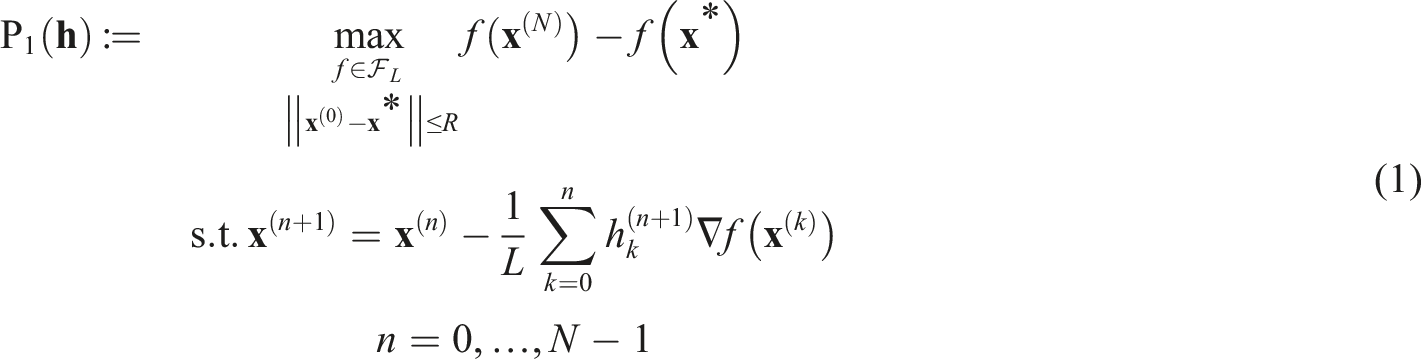
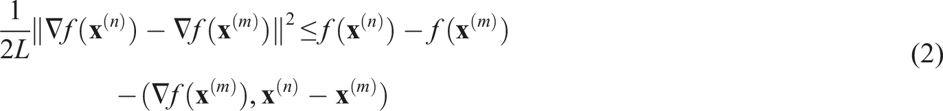
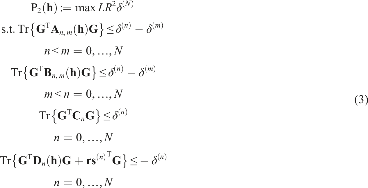
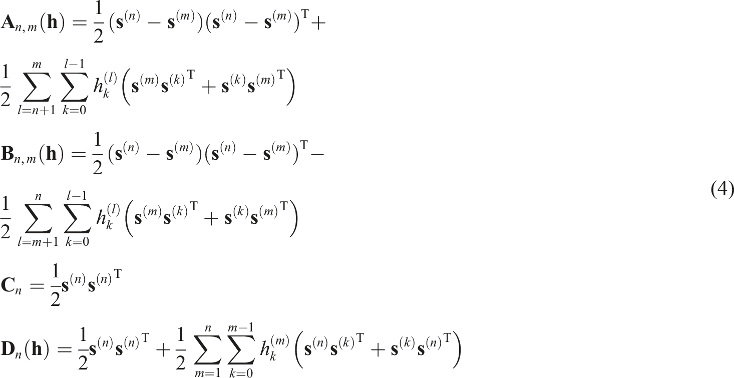
Further relaxation is to omit the middle two inequality constraints. By using Lagrange duality method, the above problem is transformed into its duality problem

${\mathrm{P}}_3\left(\mathbf{h}\right):=\min \left\{\frac{1}{2}L{R}^2\gamma :\left[\begin{array}{cc}\mathbf{S}\left(\mathbf{h},\mathit{\lambda },\mathit{\tau }\right)& \frac{1}{2}\mathit{\tau }\\ \frac{1}{2}{\mathit{\tau }}^{\mathrm{T}}& \frac{1}{2}\gamma \end{array}\right]\ge \mathbf{0}\right\}$

(5)

where elements λ, τ>0, τ⁽⁰⁾ = λ⁽¹⁾, τ^(N) + λ^(N) = 1, and λ⁽ⁿ⁾ − λ⁽ⁿ⁺¹⁾ + τ⁽ⁿ⁾ = 0, n = 1, …, N − 1, h is the parameter to be optimized. By solving the optimal parameter of the set ${\mathbf{h}}_{{\mathrm{P}}_3}=\underset{\mathbf{h}}{\text{argmin}}{\mathrm{P}}_3$ , the expression of h parameter can be obtained

$h_k^{\left(n+1\right)}=\{\begin{array}{l}\frac{1}{{\theta }^{\left(n+1\right)}}\left(2{\theta }^{\left(k\right)}-{\displaystyle \sum }_{m=k+1}^n{h}_k^{\left(m\right)}\right)\hspace{0.17em},k=0,\dots ,n-1\\ 1+\frac{2{\theta }^{\left(n\right)}-1}{{\theta }^{\left(n+1\right)}}, k=n\end{array}$

(6)

where θ⁽⁰⁾ = 1 ${\theta }^{\left(N\right)}=\left(1+\sqrt{1+8{{\theta }^{\left(N-1\right)}}^2}\right)/2$ and ${\theta }^{\left(n\right)}=\left(1+\sqrt{1+4{{\theta }^{\left(n-1\right)}}^2}\right)/2$ when 0 < n < N. The efficiency of the first-order algorithm with the above optimized parameters is equivalent to that of the following iterative form

$\begin{array}{c}\{\begin{array}{c}{\mathbf{y}}^{\left(n+1\right)}={\mathbf{x}}^{\left(n\right)}-\frac{1}{L}\nabla f\left({\mathbf{x}}^{\left(n\right)}\right)\\ {\theta }^{\left(n+1\right)}=\{\begin{array}{c}\frac{1+\sqrt{1+4{\theta }^{{\left(n\right)}^2}}}{2},n<N-1\\ \frac{1+\sqrt{1+8{\theta }^{{\left(n\right)}^2}}}{2},n=N-1\end{array}\\ {\mathbf{x}}^{\left(n+1\right)}={\mathbf{y}}^{\left(n+1\right)}+\frac{{\theta }^{\left(n\right)}-1}{{\theta }^{\left(n+1\right)}}\left({\mathbf{y}}^{\left(n+1\right)}-{\mathbf{y}}^{\left(n\right)}\right)\\ +\frac{{\theta }^{\left(n\right)}}{{\theta }^{\left(n+1\right)}}\left({\mathbf{y}}^{\left(n+1\right)}-{\mathbf{x}}^{\left(n\right)}\right)\end{array}\end{array}$

(7)

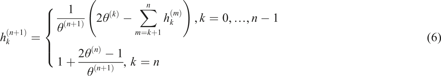
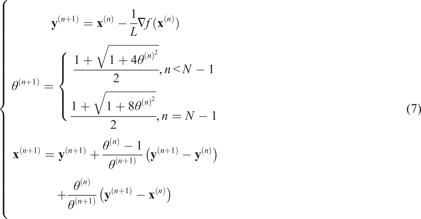
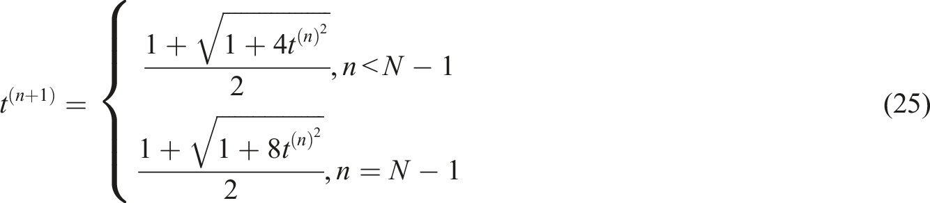
It can be seen that the designed method has two momentum terms. So, it can be called double momentum gradient (DMG) algorithm in the following.

In summary, the relaxed and dualized equation of f(x^(N)) − f(x⁽*⁾) is used to generate the optimization parameter h by using a semi-definite programming solver. The derived iterative algorithm has a tiny worst-case error boundary $f\left({\mathbf{x}}^{\left(N\right)}\right)-f\left({\mathbf{x}}^{(*)}\right)\le L{R}^2/\left(N+1\right)\left(N+1+\sqrt{2}\right)$ with an optimal rate O(1/N²) and its boundary is about half the size of Nesterov’s rapid gradient method’s worst-case boundary. As a result, the solution can be approached faster and has theoretical advantages in the first-order algorithms. In this paper, FFT and DMG are combined to solve the problem of low efficiency in deconvolution beamforming.

Improvement of deconvolution beamforming

Beamforming

When beamforming is used to locate the sound source, the pressure signal received by the microphone is first measured, and the position of the source calculation plane is divided into discrete grids. Then, the beamforming performs reverse focusing on the grid to enhance the output at the true place of the sound source, therefore locating the sound source. The schematic representation of the array setup and grid division is presented in Figure 1, assuming that the plane where the microphone is located is x-y plane and that the direction from the center of the microphone plane to the center of the source calculation plane is the z direction.

Figure 1.

Microphone array and sound source grid.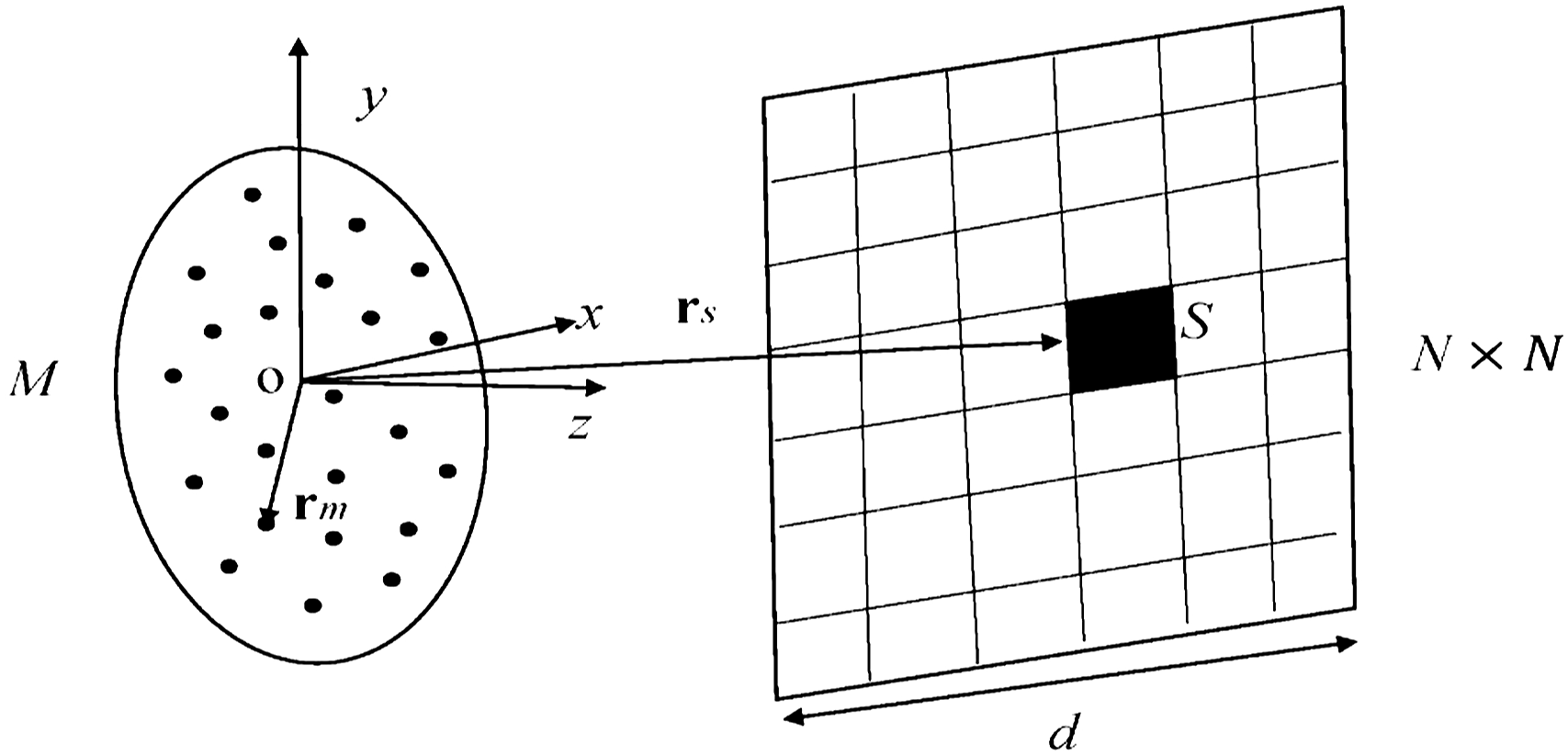

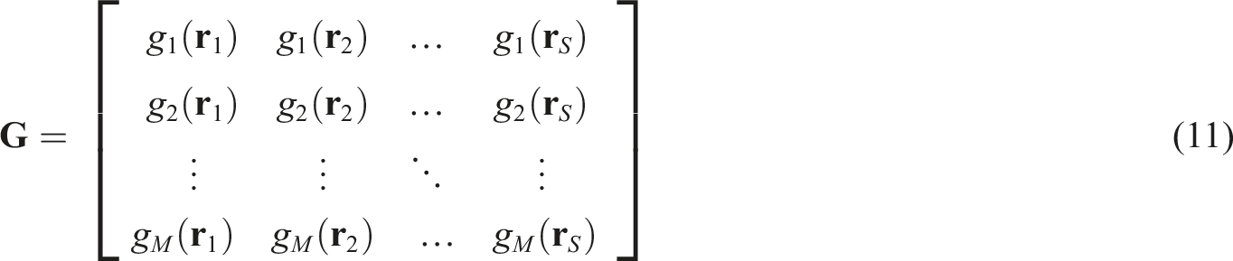
In the plane where the sound source is located, the number of grids is divided into N². Suppose a source S is at the grid, and its pressure is transmitted to M microphones. The cross-spectrum matrix required by the beamforming can be calculated using the signal collected by the sensor. For the stable signal, L _f frames measurement can be carried out before averaging. Then the expression of the cross-spectrum matrix (CSM) C at a specific frequency ω is

$\mathbf{C}\left(\omega \right)=\frac{1}{L_f}{\displaystyle \sum }_{l=1}^{L_f}{\mathbf{p}}_l\left(\omega \right){\mathbf{p}}_l{\left(\omega \right)}^{\mathrm{H}}$

(8)

where p _l (ω) is the microphone sound pressure vector of the l-th frame, and H represents conjugate transposition. According to matrix C, the output of conventional beamforming is

$b\left(\mathbf{r}\right)=\frac{1}{M^2}\mathbf{v}{\left(\mathbf{r}\right)}^{\mathrm{H}}\mathbf{C}\left(\omega \right)\mathbf{v}\left(\mathbf{r}\right)$

(9)

where v(r) is the steering vector, which is used to reverse focus the measured pressure to the grid r. The expression of the element of the steering vector is

$v_m\left(\mathbf{r}\right)=\left|\mathbf{r}-{\mathbf{r}}_m\right|\frac{e^{-\mathrm{j}k\left|\mathbf{r}-{\mathbf{r}}_m\right|}}{\left|\mathbf{r}\right|}$

(10)

where k is the wave number, |r| is the distance from the center of the microphone array to the focusing grid, and |r − r _m | is the distance from the m-th microphone to the focusing point. Equation (9) is the mean square pressure value of beamforming. The result of classic beamforming can be obtained by calculating the contributions of all focal grids. Through the above steps, the sound source can be located.

However, as previously stated, the spatial resolution of the beamforming output map is inadequate. Deconvolution beamforming can be used to improve this. The composition of cross-spectrum matrix can help us better understand the deconvolution beamforming. The process of receiving the total sound pressure is an acoustic forward process, and its propagation model is p = Gq, p = [p₁, p₂, ⋅⋅⋅, p _M ] is the amplitude vector of pressure received by the microphone, and q = [q₁, q₂, ⋅⋅⋅, q _S ] is the amplitude vector of sound sources. The expression of the Green matrix G is

$\mathbf{G}=\left[\begin{array}{c}\begin{array}{cc}\begin{array}{ccc}{g}_1\left({\mathbf{r}}_1\right)& g_1\left({\mathbf{r}}_2\right)& \dots \\ g_2\left({\mathbf{r}}_1\right)& g_2\left({\mathbf{r}}_2\right)& \dots \\ ⋮& ⋮& \ddots \end{array}& \begin{array}{c}{g}_1\left({\mathbf{r}}_S\right)\\ g_2\left({\mathbf{r}}_S\right)\\ ⋮\end{array}\end{array}\\ \begin{array}{ccc}{g}_M\left({\mathbf{r}}_1\right)& g_M\left({\mathbf{r}}_2\right)& \begin{array}{cc}\dots & g_M\left({\mathbf{r}}_S\right)\end{array}\end{array}\end{array}\right]$

(11)

where

$g_m\left({\mathbf{r}}_s\right)=\left|{\mathbf{r}}_s\right|\frac{e^{-\mathrm{j}k\left|{\mathbf{r}}_s-{\mathbf{r}}_m\right|}}{\left|{\mathbf{r}}_s-{\mathbf{r}}_m\right|}$

(12)

Then a more detailed form of sound pressure cross-spectrum matrix is obtained

$\mathbf{C}=\mathbf{G}\overline{\mathbf{q}{\mathbf{q}}^{\mathrm{H}}}{\mathbf{G}}^{\mathrm{H}}$

(13)

If sources are independent signals, the cross terms of matrix $\overline{\mathbf{q}{\mathbf{q}}^{\mathrm{H}}}$ can be ignored. The sound pressure cross-spectrum matrix can be approximated as

$\mathbf{C}={\displaystyle \sum }_{s=1}^S\overline{{\left|q_s\right|}^2}\mathbf{g}\left({\mathbf{r}}_s\right)\mathbf{g}{\left({\mathbf{r}}_s\right)}^{\mathrm{H}}$

(14)

where g(r _s ) is the column vector of the matrix G. Equation (14) establishes the relationship among cross-spectrum matrix, sound source amplitude distribution, and Green matrix. Therefore, as demonstrated in the following section, the concrete structure of the conventional beamforming output can be derived.

Deconvolution beamforming

Conventional beamforming has poor resolution, while deconvolution beamforming utilizes the relationship among conventional beamforming output, sound source amplitude distribution, and point spread function, which can greatly improve the accuracy of sound source identification and effectively improve its resolution. Substituting equation (14) into equation (9), another expression of conventional beamforming output is obtained

$b\left(\mathbf{r}\right)={\displaystyle \sum }_{s=1}^S\overline{{\left|q_s\right|}^2}psf\left(\mathbf{r}|{\mathbf{r}}_s\right)$

(15)

where psf is the point spread function, which is the response of beamforming output to the unit power of sound source

$psf\left(\mathbf{r}|{\mathbf{r}}_s\right)=\frac{1}{M^2}\mathbf{v}{\left(\mathbf{r}\right)}^{\mathrm{H}}\mathbf{g}\left({\mathbf{r}}_s\right)\mathbf{g}{\left({\mathbf{r}}_s\right)}^{\mathrm{H}}\mathbf{v}\left(\mathbf{r}\right)$

(16)

The output of conventional beamforming is the convolution of sound source amplitude and point spread function. Deconvolution beamforming uses this relationship to create a linear equation set that extracts the true sound source information while effectively removing the effects of sidelobe interference and main lobe width. The equation (15) is vectorized and transformed into the form of the multiplication of matrix and vector, and then

$\mathbf{b}=\mathbf{A}\mathbf{x}$

(17)

where b is an N²-dimensional column vector composed of b(r), A is an N² × N²-dimensional matrix composed of psf(r|r _s ), and the x vector is composed of |q _s |², and the vector is non-negative. The solving process of vector x is a linear inverse problem

$\begin{array}{c}\text{minimize}\hspace{1em}\frac{1}{2}\Vert \mathbf{b}-\mathbf{A}\mathbf{x}{\Vert }_2^2\\ \mathrm{s}.\mathrm{t}.\hspace{1em}{x}_i\ge 0\end{array}$

(18)

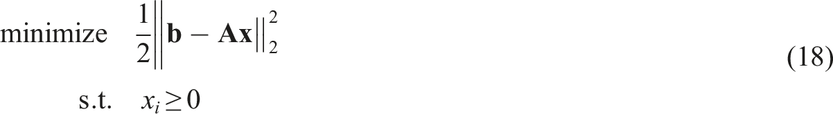
The optimization problem in equation (18) is also called the non-negative least squares problem, which can be solved by the first-order algorithm.

FFT-DMG

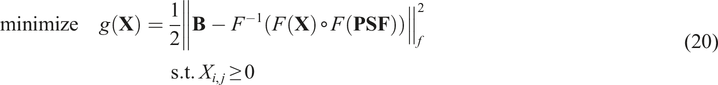
In order to improve the efficiency of deconvolution beamforming, in this section, Fourier algorithm is firstly used to transform convolution operation into Hadamard product of matrix, and then double momentum gradient algorithm is used to further improve the calculation efficiency.

Based on the assumption that point spread function is shift-invariant, ³⁷ equation (17) is calculated in wavenumber domain by discrete spatial fast Fourier transform, and the expression of matrix form is as follows

$\mathbf{B}=\mathbf{X}*\mathbf{P}\mathbf{S}\mathbf{F}=F^{-1}\left(F\left(\mathbf{X}\right)\circ F\left(\mathbf{P}\mathbf{S}\mathbf{F}\right)\right)$

(19)

Each matrix has the same dimension N × N. * is convolution symbol, $\circ$ is Hadamard product. F⁻¹ is the two-dimensional inverse Fourier transform and F is the two-dimensional Fourier transform. With this transformation, the computational efficiency is improved. That is, compared to a $\mathcal{O}\left(N^4\right)$ time complexity of the matrix-vector multiplication Ax, the Fourier transform can be performed via a circular convolution with the FFT in $\mathcal{O}\left(2N^{2}logN\right)$ time complexity for the N² computational grid. According to equation (19), the non-negative least squares problem in equation (18) can be rewritten as

$\begin{array}{c}\text{minimize}\hspace{1em}g\left(\mathbf{X}\right)=\frac{1}{2}\Vert \mathbf{B}-F^{-1}\left(F\left(\mathbf{X}\right)\circ F\left(\mathbf{P}\mathbf{S}\mathbf{F}\right)\right){\Vert }_f^2\\ \mathrm{s}.\mathrm{t}. X_{i,j}\ge 0\end{array}$

(20)

where ||⋅|| _f represents the F norm of matrix. Because it avoids the explicit expression of A, this method greatly reduces the calculation running time. In order to further improve the calculation efficiency of solving equation (20), the first-order algorithm with optimized parameter h is adopted. The main iterative process is as follows

$\begin{array}{c}\nabla g\left({\mathbf{X}}^{\left(n\right)}\right)\\ =F^{-1}\left(F\left(\mathbf{P}\mathbf{S}{\mathbf{F}}^T\right)\circ F\left(F^{-1}\left(F\left({\mathbf{X}}^{\left(n\right)}\right)\circ F\left(\mathbf{P}\mathbf{S}\mathbf{F}\right)\right)-\mathbf{B}\right)\right)\end{array}$

(21)

Update variable Y

${\mathbf{Y}}^{\left(n+1\right)}={\mathbf{X}}^{\left(n\right)}-\nabla g\left({\mathbf{X}}^{\left(n\right)}\right)/L$

(22)

Calculate momentum terms A and B

${\mathbf{A}}^{\left(n+1\right)}={\mathbf{Y}}^{\left(n+1\right)}-{\mathbf{Y}}^{\left(n\right)}$

(23)

${\mathbf{B}}^{\left(n+1\right)}={\mathbf{Y}}^{\left(n+1\right)}-{\mathbf{X}}^{\left(n\right)}$

(24)

Update inertia sequence t

$t^{\left(n+1\right)}=\{\begin{array}{c}\frac{1+\sqrt{1+4t^{{\left(n\right)}^2}}}{2},n<N-1\\ \frac{1+\sqrt{1+8t^{{\left(n\right)}^2}}}{2},n=N-1\end{array}$

(25)

Update variable X

${\mathbf{X}}^{\left(n+1\right)}=P_{+}\left({\mathbf{Y}}^{\left(n+1\right)}+\frac{t^{\left(n\right)}-1}{t^{\left(n+1\right)}}{\mathbf{A}}^{\left(n+1\right)}+\frac{t^{\left(n\right)}}{t^{\left(n+1\right)}}{\mathbf{B}}^{\left(n+1\right)}\right)$

(26)

Simulation

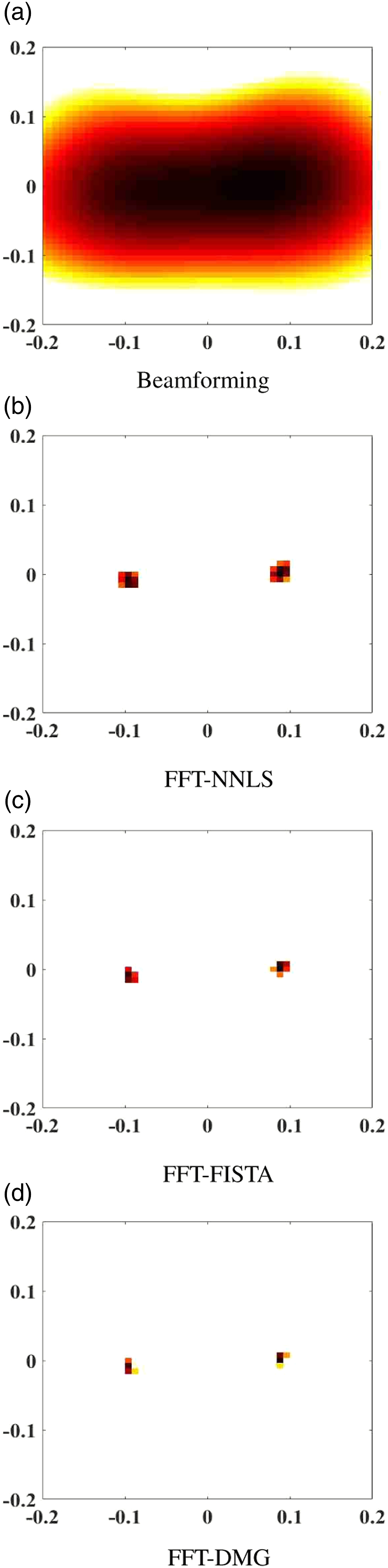
In the section, the virtual simulation of two-point sound sources is carried out. The focus is to investigate the computational efficiency of the proposed method for deconvolution beamforming. The performances of FFT-NNLS, FFT-FISTA, and FFT-DMG are evaluated and compared in both resolution and running time. Two-unit power point sound sources are placed in the x-y plane with the coordinates of (0.1,0) m and (−0.1,0) m, and 0.4 m away from a plane 18-channel microphone array. The microphone array is a pseudo-random array with a diameter of 0.38 m. White Gaussian noise with an SNR of 30 dB is added. Take 2000 Hz as an example. Set the grid number in source calculation surface to N × N = 51 × 51 = 2601. The number of iterations is 3000. The calculated sound source map is shown in Figure 2. Sound sources can be well identified and located by deconvolution beamforming. It can be seen that FFT-DMG has the smallest main lobe, and its sound source localization ability is better than FFT-FISTA and FFT-NNLS.

Figure 2.

Sound sources location map in simulation.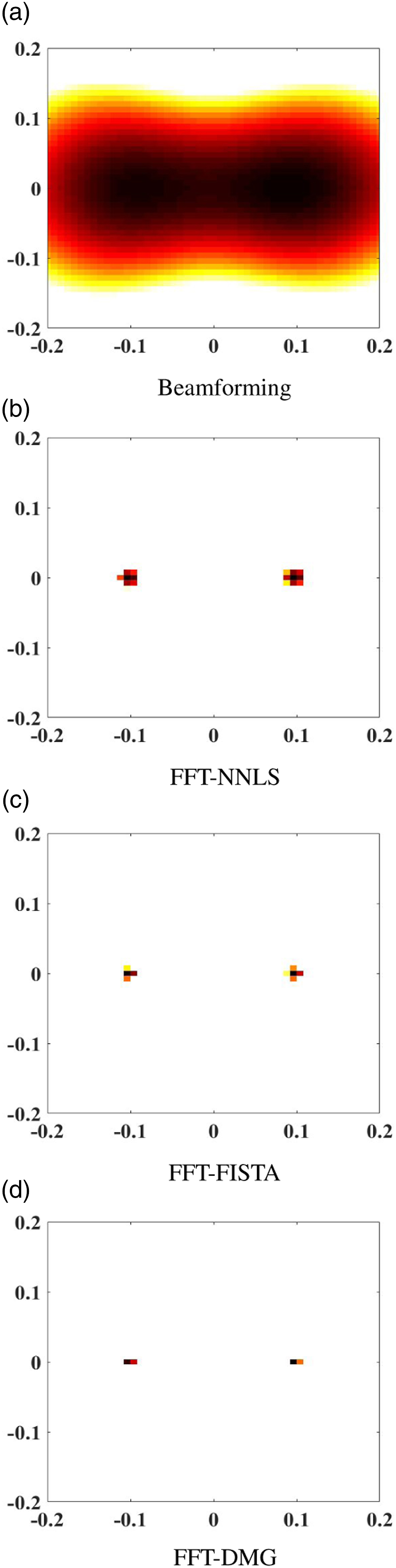

To compare the convergence efficiency of different algorithms, the proportional parameter R ¹⁸ is defined

$\mathrm{R}=\frac{g\left({\mathbf{X}}^{\left(n\right)}\right)-g\left({\mathbf{X}}^{(*)}\right)}{g\left({\mathbf{X}}^{(*)}\right)}$

(27)

where g(X⁽*⁾) is the optimal value. It can be seen that the smaller R is, the more accurate the identification is. According to the parameter R, the convergence process of different algorithms can be clearly observed.

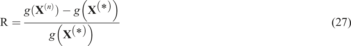
Figure 3 shows the relationship between the parameter R and the iteration number k on a logarithmic scale. At first, FFT-NNLS, FFT-FISTA, and FFT-DMG algorithms have relatively close convergence properties. However, the iterative curve of FFT-NNLS suddenly has a peak at the 203rd iteration. This intermittent fluctuation continued until the 404th iteration. The FFT-NNLS gradually stabilized after violent fluctuation. Finally, after 421 iterations, the convergence performance of FFT-NNLS cannot continue to improve, and it is in a stagnant state. The convergence performance of the latter two methods is better. After 3000 iterations, they can obtain good calculation accuracy.

Figure 3.

R values as a function of iterations.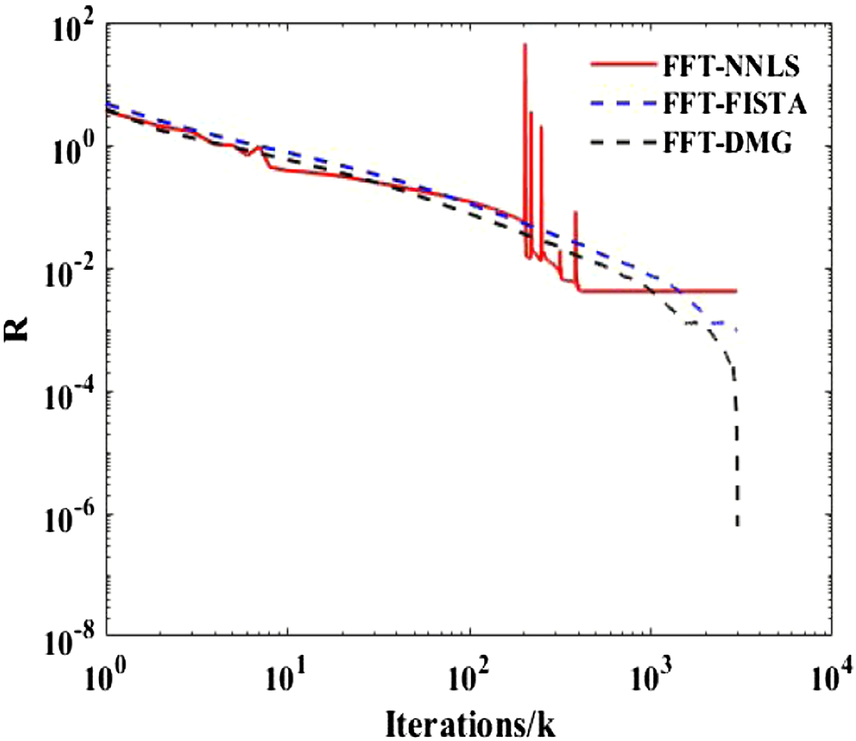

The efficiency of computation is a major concern. To visually display the running time of all algorithms, the iteration time of each algorithm with iteration number k is compared and analyzed, as shown in Figure 4. The processor used in the simulation condition is Intel Core(TM) i5-7500 CPU 3.0 GHz. After three thousand iterations, the FFT-NNLS takes 5.3170 s, and the FFT-FISTA and FFT-DMG take 3.2926 s and 3.2855 s. Each iteration of FFT-NNLS takes about 1.7723 ms, and each iteration of FFT-FISTA and FFT-DMG takes about 1.0975 ms and 1.0952 ms. It can be seen that FFT-FISTA and FFT-DMG save 38.07% and 38.21% time than FFT-NNLS. They can perform more iterations than FFT-NNLS in the same time. The extra time used by FFT-NNLS is due to the calculation of step size in each iteration. The step size in FFT-DMG is set by optimization before, so there is no need for extra time for each iteration. Compared to FFT-FISTA, in terms of each iteration time, FFT-DMG appears to have no obvious advantage. However, the real concern is the time taken by the algorithm to reach the same precision.

Figure 4.

Time values as a function of iterations.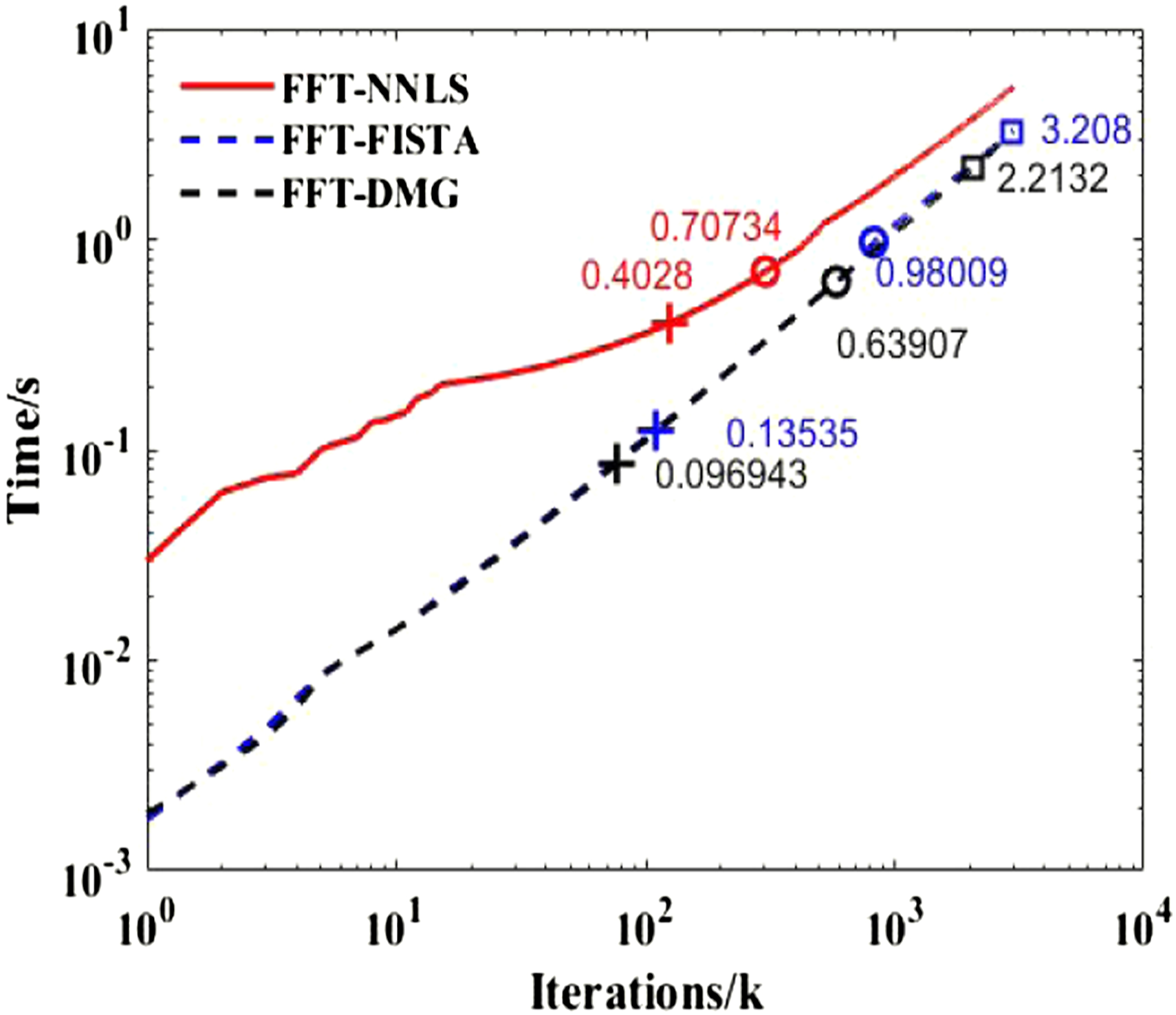

In Figure 4, the same precision is marked. (R = 0.1 (cross), R = 0.01 (circle) and R = 0.001 (square). It is more exact to go smaller.) Comparing FFT-NNLS with FFT-FISTA, we can find that the parameter R of FFT-NNLS can converge to 0.01 faster than FFT-FISTA. It means that even if FFT-FISTA takes less time for each iteration, the R value of FFT-NNLS can reach 0.01 in a shorter time and with fewer iterations. At 1435 iterations, the accuracy of FFT-FISTA is better than that of FFT-NNLS. In the above methods, the proposed FFT-DMG algorithm has better properties. Firstly, compared with FFT-NNLS algorithm, FFT-DMG needs shorter time for each iteration. Secondly, compared with FFT-FISTA, FFT-DMG can achieve the same accuracy with fewer iterations. When the parameter R is 0.1, 0.01, and 0.001, FFT-DMG is 28.38%, 34.79%, and 31.01% faster than FFT-FISTA, respectively. Among these three algorithms, FFT-DMG algorithm is the best in efficiency, which can identify sound source with the fastest speed and high quality. Notably, in the simulation, the number of grids is set to 2601, but in practical applications (such as in wind tunnels), the number of grids is very large, and the efficiency advantage of the proposed algorithm is more obvious.

In addition, we compare the computational efficiency of the methods at different frequencies and analyze the performance of the methods in high background noise conditions, as shown in Figures 5 and 6. Figure 5(a) shows the total time of 3000 iterations of each method. Figure 5(b)–(d) show the time taken under different R values. Black color of the colorbar indicates that the accuracy has not been reached during the 3000 iterations. It can be seen that, consistent with the previous analysis, the time used for FFT-FISTA and FFT-DMG is significantly reduced for the same number of iterations. Besides, the average time taken at all frequencies is calculated. Compared with FFT-FISTA, FFT-DMG can save 29.48% (R = 0.1), 29.05% (R = 0.01), and 28.94% (R = 0.001) of the computational time, respectively. Figure 6 shows the location map of 2000 Hz under the condition of low signal-to-noise ratio (SNR = 0 dB). It can be seen that due to noise interference, deconvolution methods are affected to some extent. This is because noise has an impact on the result of beamforming, and deconvolution beamforming is calculated on the basis of the beamforming. Therefore, when the CSM of beamforming is processed by noise reduction method (e.g., diagonal removal or diagonal reconstruction Ref. [38,39]), the robustness of the beamforming method to noise can be improved. Then the robustness of the deconvolution method to noise can also be improved.

Figure 5.

The time taken for sound source localization in simulation.

Figure 6.

Sound sources location map under high background noise conditions. (SNR = 0 dB).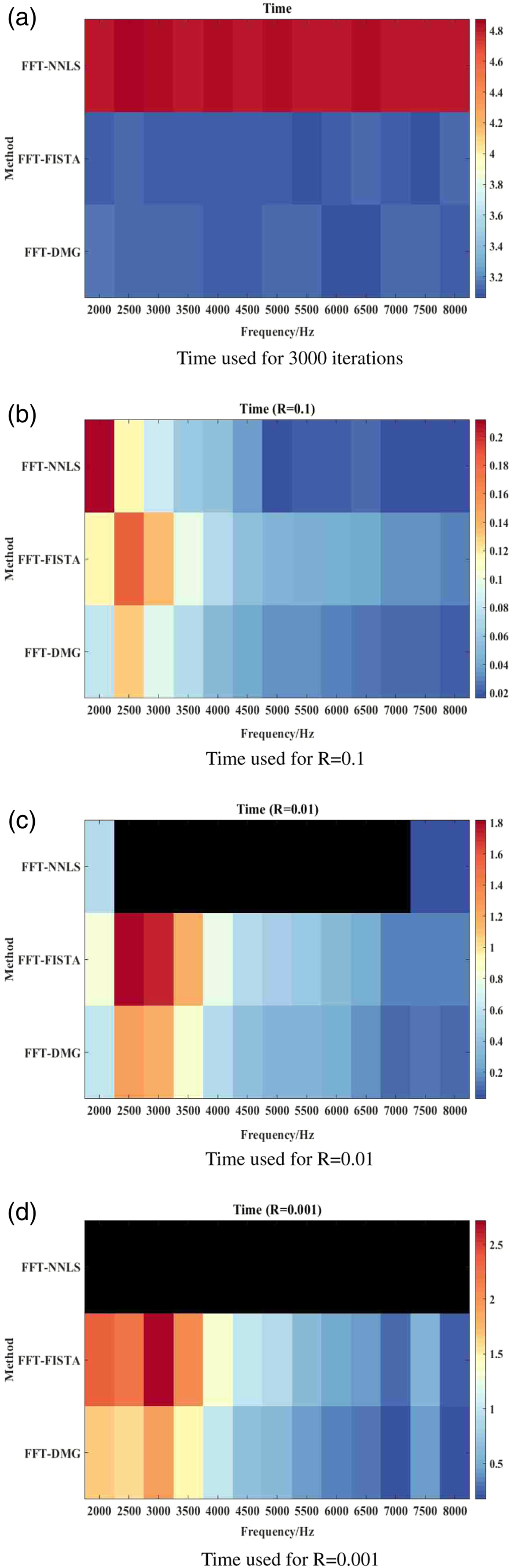

Experimental verification

In order to verify the correctness of the simulation, experimental verification is carried out. The experiment is conducted in an ordinary room. The 18-channel pseudo-random microphone array of HBK company and its matching collector are used. Set the center position of microphone array as the origin. Loudspeakers are arranged at the coordinates of (0.1,0,0.4) m and (−0.1,0,0.4) m. The sampling frequency is 16,384 Hz, and the total sampling time is 5 s. Figure 7 shows the layout of the experiment.

Figure 7.

Experiment layout.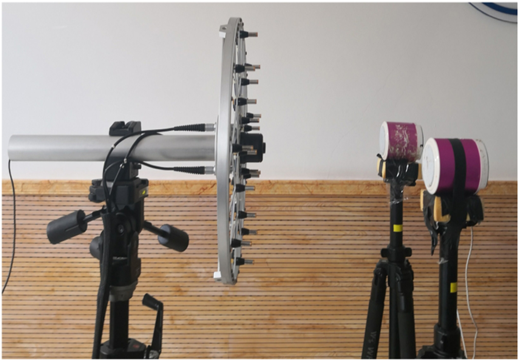

Apply FFT-NNLS, FFT-FISTA, and FFT-DMG algorithms to post-process the collected signals. The number of iterations is also 3000 times. Figure 8 shows the location results of the experiment. The sound source is clearly identified at the position where the loudspeaker is arranged. Compared with FFT-NNLS and FFT-FISTA algorithms, FFT-DMG has a certain improvement in resolution.

Figure 8.

Sound sources location map in experiment.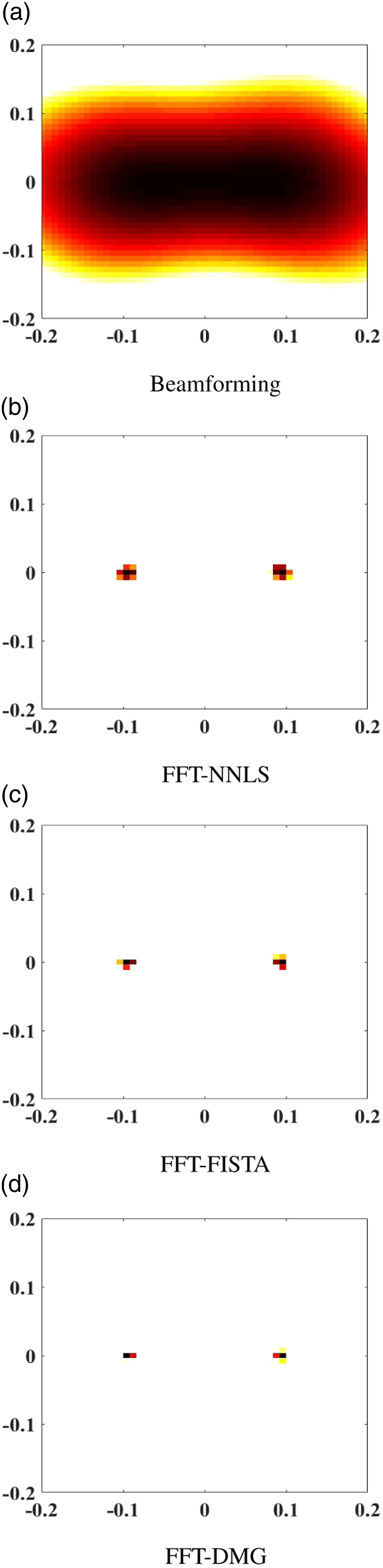

The parameter R is also used to evaluate the convergence property. Figure 9 shows the variation of the parameter R with the number of iterations k in experiment. It can be seen that under the same number of iterations, the convergence speed of FFT-DMG algorithm is the fastest and the decline is the most obvious. This proves the reason why this algorithm has advantages in the localization of sound sources.

Figure 9.

R values as a function of iterations.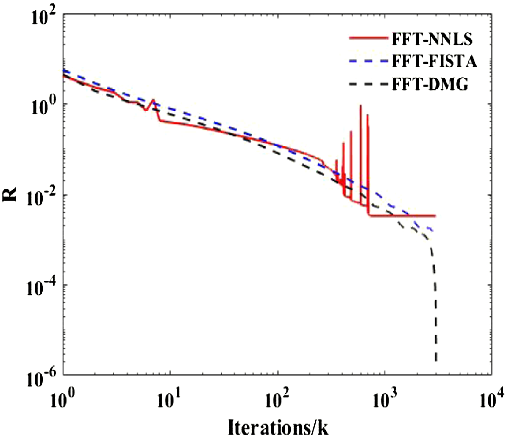

Figure 10 can compare the convergence efficiency of the algorithm more intuitively. First of all, according to 3000 iterations, FFT-NNLS, FFT-FISTA and FFT-DMG algorithms take 5.3311 s, 3.3191 s, and 3.2425 s, respectively. The average iteration time is 1.7770 ms, 1.1064 ms, and 1.0808 ms, respectively. FFT-FISTA and FFT-DMG are about 37.74% and 39.18% faster than FFT-NNLS. From this point of view, there is little difference in average iteration time between FFT-FISTA and FFT-DMG. Then the calculation time when the same accuracy is achieved is analyzed.

Figure 10.

Time values as a function of iterations.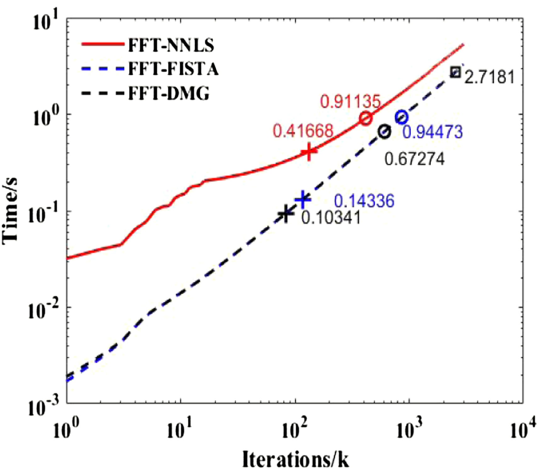

It can be seen that the convergence speed of FFT-DMG is always the fastest when reaching the same precisions. When the convergence parameter R reaches 0.1, FFT-DMG can save about 75.18% time compared with FFT-NNLS and about 27.87% time compared with FFT-FISTA. When the convergence parameter R reaches 0.01, FFT-DMG can save about 26.18% time compared with FFT-NNLS and about 28.79% time compared with FFT-FISTA. In addition, it can be seen that although the average iteration time of FFT-FISTA is faster than that of FFT-NNLS, the time FFT-FISTA used when R = 0.01 is longer than that of FFT-NNLS algorithm, which means that FFT-FISTA algorithm uses more iteration steps. Within 3000 iterations, only the R of FFT-DMG can reach 0.001. Figure 11 shows the comparison of computational efficiency at different frequencies in the experiment. The experiment is similar to the simulation. The R value of FFT-NNLS cannot reach 0.001 at these frequencies. The average time taken at all frequencies is also calculated. Compared with FFT-FISTA, FFT-DMG can save 29.70% (R = 0.1), 32.83% (R = 0.01), and 31.22% (R = 0.001) of the computational time, respectively. Therefore, through the analysis of computational efficiency, it can be noticed that the iterative efficiency of FFT-DMG is the best, and it is superior to FFT-NNLS and FFT-FISTA algorithms in time statistics.

Figure 11.

The time taken for sound source localization in experiment.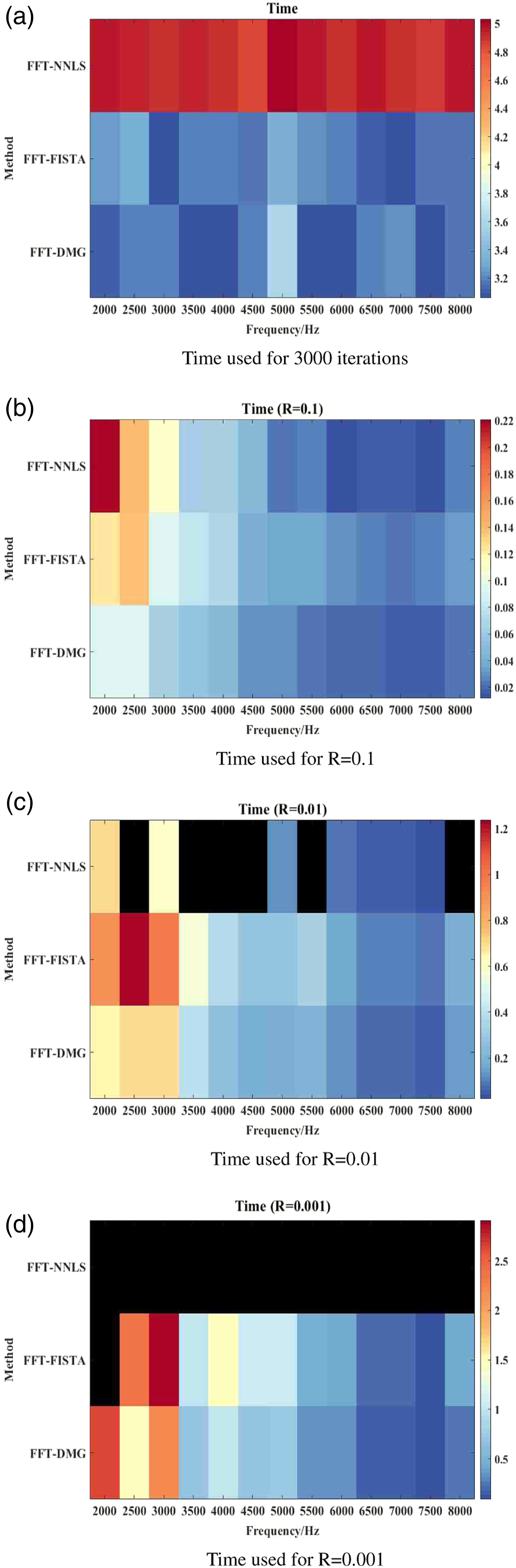

Conclusion

In order to improve the computational efficiency of deconvolution beamforming, a deconvolution method based on FFT-DMG algorithm is proposed. It can improve the computational efficiency of deconvolution beamforming and has good computational accuracy.

The performance of the proposed method is compared and verified with FFT-NNLS and FFT-FISTA algorithms. It is found that FFT-DMG algorithms take less time per iteration than FFT-NNLS on average, and can save approximately 40% of the calculation time. In addition, when the accuracy of the FFT-FISTA and FFT-DMG algorithms is consistent, the calculation time of FFT-DMG can be reduced by approximately 30%.

When all algorithms use the same number of iterations, FFT-DMG tends to provide solutions with a better spatial resolution than FFT-FISTA and FFT-NNLS. This feature makes the proposed method more advantageous in applications with a huge number of grids. Therefore, compared with FFT-NNLS and FFT-FISTA algorithms, FFT-DMG algorithm can achieve better calculation results in a shorter time, and has certain application value.