High-resolution CLEAN-SC: Theory and experimental validation

Abstract

In this article, a high-resolution extension of CLEAN-SC is proposed: high-resolution-CLEAN-SC. Where CLEAN-SC uses peak sources in ‘dirty maps’ to define so-called source components, high-resolution-CLEAN-SC takes advantage of the fact that source components can likewise be derived from points at some distance from the peak, as long as these ‘source markers’ are on the main lobe of the point spread function. This is very useful when sources are closely spaced together, such that their point spread functions interfere. Then, alternative markers can be sought in which the relative influence by point spread functions of other source locations is minimised. For those markers, the source components agree better with the actual sources, which allows for better estimation of their locations and strengths. This article outlines the theory needed to understand this approach and discusses applications to 2D and 3D microphone array simulations with closely spaced sources. An experimental validation was performed with two closely spaced loudspeakers in an anechoic chamber.

Introduction

Location of acoustic sources by phased array beamforming is subject to spatial resolution bounds, i.e. sources which are too close to each other cannot be resolved. The conventional beamforming (CB) method ¹ is limited by the Rayleigh criterion, ² which describes the minimum spacing between two resolvable sources as a function of array aperture and frequency. A further restriction of the application of CB is set by the dynamic range ¹ of the array, which is the maximum level difference between the peak source and other detectable sources. The first step towards minimisation of these limitations is the design of appropriate array patterns.^3,4 To obtain further enhancements in spatial resolution and dynamic range, deconvolution methods like DAMAS ⁵ and high-resolution methods like Functional Beamforming ⁶ have been proposed.

A well-known deconvolution technique is CLEAN-SC. ⁷ This method starts with an acoustic image obtained with CB and features the iterative removal of those parts of the acoustic image that are coherent with the peak source. For each iteration step, the removed part of the image is related to a ‘source component’, which estimates measured microphone data due to a single coherent source. Each source component is represented by an artificial ‘clean beam’ at the peak location in a new acoustic image: the ‘clean map’. The levels of the clean beams are calculated from the source components.

An advantage of CLEAN-SC, compared to other advanced beamforming methods, is its low sensitivity to errors made in the source model that describes sound propagation from potential sources to microphones. Another convenient feature is that the determination of source components is not very sensitive to the location that is marked as peak. In other words, if the scan grid is too coarse or if it is out of focus, a small error may be made in the peak location, but the corresponding source levels remain correct. Thus, CLEAN-SC provides levels at a higher reliability than CB.

CLEAN-SC is an appropriate tool for determining acoustic sources within a large range of levels, not being limited to the conventional dynamic range. On the other hand, it does not provide a spatial resolution beyond the Rayleigh limit. If two sources are too close to each other, the CB peak location is somewhere in between both sources, and the corresponding CLEAN-SC source component is a linear combination of the two individual sources.

In those cases, it can be advantageous to move the ‘source marker’ away from the actual peak location, to a location where the CB result is dominated by either one of the sources (see Figure 1). The thus obtained source components are significantly better estimates of the array data from the true sources. Improved estimations of the locations of the sources are obtained by applying CB to the improved source components.

Figure 1.

Sketch of the main idea of HR-CLEAN-SC.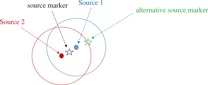

To determine the best marker locations, knowledge about the actual source locations is required. But these locations are not always known a priori. However, we will demonstrate that an iterative procedure, starting with the standard CLEAN-SC solution, also leads to an increase in resolution, based on the idea of optimising marker locations.

In the following section, the theory is outlined. In ‘Simulated array data’ section, applications to 2D and 3D microphone array simulations with closely spaced sources are discussed. ‘Experimental validation’ section describes an experimental validation with two loudspeaker sources. The conclusions are summarised in the final section.

Theory

The cross-spectral matrix (CSM)

The starting point for frequency-domain beamforming methods with microphone arrays is the CSM. It is assumed here that the CSM can be written as a summation of contributions from K incoherent sources:

$$\begin{array}{c}\multicolumn{1}{c}{\mathbf{C}=\sum _{k=1}^K{\mathbf{p}}_k{\mathbf{p}}_k^{*}.}\end{array}$$

(1)

Herein, ${\mathbf{p}}_k$ are N-dimensional ‘source vectors’ (N being the number of microphones) representing the Fourier transforms of the signals from the k-th source. The asterisk stands for the complex conjugate transpose. The assumption of equation (1) is valid under the following conditions:

The CSM is calculated from a large number of time blocks, so that the ensemble averages of the cross-products ${\mathbf{p}}_k{\mathbf{p}}_l^{*},k\ne l$ , can be neglected.

There is no decorrelation of signals from the same source between different microphones (e.g. due to sound propagation through turbulence).

There is no additional incoherent noise.

Steering vectors

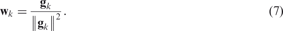
Beamforming methods make use of ‘steering vectors’ $\mathbf{g}\in {ℂ}^{N\times 1}$ . These vectors contain the microphone array responses of potential sources. It is quite common to assume point sources represented by free-field Green’s functions of the Helmholtz equation. Then the n-th element of g reads

$$\begin{array}{c}\multicolumn{1}{c}{g_n(\overrightarrow{\xi })=\frac{-1}{4\pi \Vert {\overrightarrow{x}}_n-\overrightarrow{\xi }\Vert }\exp (\frac{-2\pi \mathrm{if}\Vert {\overrightarrow{x}}_n-\overrightarrow{\xi }\Vert }{c}),}\end{array}$$

(2)

where f is the frequency, c the sound speed, ${\overrightarrow{x}}_n$ the position of the n-th microphone and $\overrightarrow{\xi }$ the source location. However, g can represent any sound source mechanism, like plane waves or point sources with non-uniform directivity, or extended source regions. Also, it can include acoustic propagation through non-uniform media. ⁸

For beamforming, a so-called ‘scan grid’ is defined, which is basically a set of steering vectors coupled to potential sources. The scan grid should comprise all sources that produce the CSM. It is favourable, in general, to implement the most accurate representation of the physics into the steering vectors, in other words, to maximise the likelihood of steering vectors g being proportional to the source vectors ${\mathbf{p}}_k$ . Ideally, the scan grid contains steering vectors ${\mathbf{g}}_k$ that are exactly proportional to the source vectors:

$$\begin{array}{c}\multicolumn{1}{c}{{\mathbf{p}}_k=a_k{\mathbf{g}}_k,}\end{array}$$

(3)

where a_k is a (complex-valued) source amplitude.

For actual array measurements, however, there is usually no exact proportionality. Deviations between actual source vectors and theoretical steering vectors can be due to the source not being a true point source, a non-uniform directivity, errors in the scan grid, errors in the microphone locations, errors in the sound propagation model or errors in the microphone sensitivity.

The aim of beamforming is to detect sources and to determine associated source powers, i.e. to decompose the CSM like

$$\begin{array}{c}\multicolumn{1}{c}{\mathbf{C}\approx \sum _{k=1}^K{A}_k{\mathbf{g}}_k{\mathbf{g}}_k^{*}.}\end{array}$$

(4)

For ideal source vectors ${\mathbf{p}}_k$ , for which equation (3) holds, the source powers A_k must be

$$\begin{array}{c}\multicolumn{1}{c}{A_k=|a_k{|}^2.}\end{array}$$

(5)

CB

The expression for calculating source power estimates with CB is

$${\tilde{A}}_k={\mathbf{w}}_k^{*}{\mathbf{Cw}}_k,$$

(6)

featuring the ‘weight vector’ ${\mathbf{w}}_k$ :

$${\mathbf{w}}_k=\frac{{\mathbf{g}}_k}{\Vert {\mathbf{g}}_k{\Vert }^2}.$$

(7)

Application of CB to the CSM assumed in equation (1) yields

$$\begin{array}{c}\multicolumn{1}{c}{{\tilde{A}}_k={\mathbf{w}}_k^{*}(\sum _{j=1}^K{\mathbf{p}}_j{\mathbf{p}}_j^{*}){\mathbf{w}}_k=\sum _{j=1}^K|{\mathbf{p}}_j^{*}{\mathbf{w}}_k{|}^2.}\end{array}$$

(8)

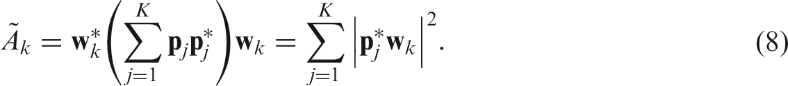
For ideal source vectors, equation (3), we have

$${\tilde{A}}_k=A_k+\sum _{\genfrac{}{}{0ex}{}{j=1}{j\ne k}}^K{A}_j|{\mathbf{g}}_j^{*}{\mathbf{w}}_k{|}^2.$$

(9)

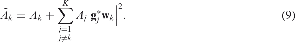
Equation (9) provides a good source power estimate for source k when the j-summation in the right-hand side is relatively small. If the sources $j\ne k$ have powers A_j that are comparable to A_k, then it is desirable to have

$$\begin{array}{c}\multicolumn{1}{c}{|{\mathbf{g}}_j^{*}{\mathbf{w}}_k{|}^2<<1.}\end{array}$$

(10)

The expression in the left-hand side of equation (10) is known as the ‘point spread function’ (PSF) of source j. Equation (10) states that the sources j and k must be sufficiently far away from each other, and that side lobes of the PSF should be small.^3,4 The PSF characteristics thus limit the application of CB. The aim of deconvolution methods, like the ‘CLEAN’ methods discussed in the next section, is essentially to correct for the PSFs.

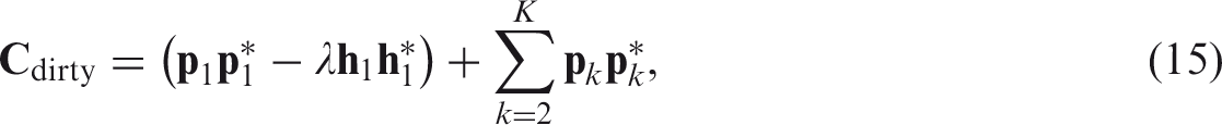
CLEAN-PSF and CLEAN-SC

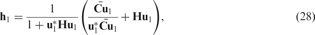
The classical CLEAN ⁹ deconvolution algorithm (referred to as ‘CLEAN-PSF’ in the CLEAN-SC publication ⁷ ) works as follows. Let ${\mathbf{p}}_1$ be the highest level source vector and ${\mathbf{g}}_1$ the best matching steering vector (e.g. found as the one for which CB yields the maximum source power estimate). Then the CSM is rewritten as follows:

$$\mathbf{C}={\mathbf{C}}_{\text{clean}}+{\mathbf{C}}_{\text{dirty}},$$

(11)

with

$${\mathbf{C}}_{\text{clean}}=\lambda {\mathbf{g}}_1{\mathbf{g}}_1^{*},$$

(12)

$${\mathbf{C}}_{\text{dirty}}=({\mathbf{p}}_1{\mathbf{p}}_1^{*}-\lambda {\mathbf{g}}_1{\mathbf{g}}_1^{*})+\sum _{k=2}^K{\mathbf{p}}_k{\mathbf{p}}_k^{*},$$

(13)

where λ is the source power estimate ${\tilde{A}}_1$ multiplied with a loop gain or damping factor ⁹ between 0 and 1. The ${\mathbf{C}}_{\text{clean}}$ results, featuring a source location associated with ${\mathbf{g}}_1$ and a corresponding amplitude, are coupled to a ‘clean map’, while ${\mathbf{C}}_{\text{dirty}}$ is used as input for the next iteration step.

The CLEAN-SC ⁷ counterparts of equations (12) and (13) are

$${\mathbf{C}}_{\text{clean}}=\lambda {\mathbf{h}}_1{\mathbf{h}}_1^{*},$$

(14)

$${\mathbf{C}}_{\text{dirty}}=({\mathbf{p}}_1{\mathbf{p}}_1^{*}-\lambda {\mathbf{h}}_1{\mathbf{h}}_1^{*})+\sum _{k=2}^K{\mathbf{p}}_k{\mathbf{p}}_k^{*},$$

(15)

with the ‘source component’ ${\mathbf{h}}_1$ defined by

$$\begin{array}{c}\multicolumn{1}{c}{{\mathbf{h}}_1=\frac{{\mathbf{Cw}}_1}{{\mathbf{w}}_1^{*}{\mathbf{Cw}}_1}=\frac{{\mathbf{p}}_1^{*}{\mathbf{w}}_1}{{\tilde{A}}_1}\{{\mathbf{p}}_1+\frac{1}{{\mathbf{p}}_1^{*}{\mathbf{w}}_1}\sum _{k=2}^K({\mathbf{p}}_k^{*}{\mathbf{w}}_1){\mathbf{p}}_k\},}\end{array}$$

(16)

where ${\mathbf{w}}_1$ is the weight vector associated with ${\mathbf{g}}_1$ via equation (7). The source component ${\mathbf{h}}_1$ can be regarded as an improved version of the steering vector ${\mathbf{g}}_1$ , being more proportional to the unknown source vector ${\mathbf{p}}_1$ .

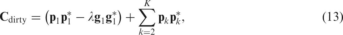
If the best-matching steering vector ${\mathbf{g}}_1$ is proportional to the source vector, then CLEAN-PSF is a perfect deconvolution method, since the contribution of the principal source ${\mathbf{p}}_1$ can be removed completely from the ‘dirty’ CSM, equation (13). With the right choice for λ, the first term in the right-hand side of (13) can be completely annihilated. This does not hold for CLEAN-SC. For proportional ${\mathbf{g}}_1$ and ${\mathbf{p}}_1$ (ideal source vectors), we obtain for the source component:

$$\begin{array}{c}\multicolumn{1}{c}{{\mathbf{h}}_1=\frac{A_1}{{\tilde{A}}_1}\{{\mathbf{g}}_1+\frac{1}{A_1}\sum _{k=2}^K{A}_k({\mathbf{g}}_k^{*}{\mathbf{w}}_1){\mathbf{g}}_k\}.}\end{array}$$

(17)

Thus, the dirty CSM gets polluted by contributions of the principal source. These contributions, however, can be relatively small, depending on the values of ${\mathbf{g}}_k^{*}{\mathbf{w}}_1$ , i.e. on the PSF values.

In the non-ideal case, when ${\mathbf{g}}_1$ is not proportional to ${\mathbf{p}}_1$ , the dirty matrix obtained with CLEAN-PSF, equation (13) can contain significant contributions of ${\mathbf{p}}_1$ . On the other hand, with CLEAN-SC, no additional errors are introduced when equation (17) is replaced by equation (16). This is one of the main advantages of CLEAN-SC compared to other deconvolution methods, namely that it does not lose performance if the steering vectors do not exactly match with source vectors.

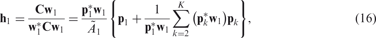
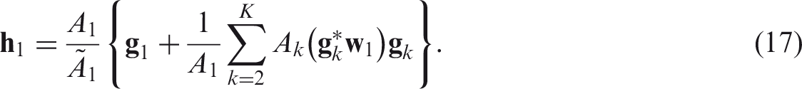
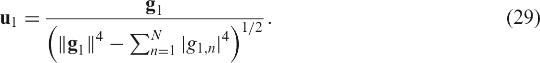
High-resolution CLEAN-SC

The fact that the best-matching steering vector ${\mathbf{g}}_1$ and the source vector ${\mathbf{p}}_1$ do not need to be proportional can be exploited for optimising the CLEAN-SC results. The source component ${\mathbf{h}}_1$ , equation (16), provides the best (proportional) estimate for ${\mathbf{p}}_1$ if the second term between the brackets in the right-hand side of equation (16) is minimised relative to the first term. This is realised by minimising the following cost function:

$$F({\mathbf{u}}_1)=\frac{\Vert \sum _{k=2}^K({\mathbf{p}}_k^{*}{\mathbf{u}}_1){\mathbf{p}}_k{\Vert }^2}{|{\mathbf{p}}_1^{*}{\mathbf{u}}_1{|}^2·\Vert {\mathbf{p}}_1{\Vert }^2},$$

(18)

where ${\mathbf{u}}_1$ is the weight vector ( ${\mathbf{w}}_1$ ) associated with an alternative ‘source marker’, as discussed in the ‘Introduction’ section. Basically, this cost function minimises the influence that other sources have on the CB result of the peak source. Obviously, not only the peak source needs to have minimum influence by other sources, the same holds for any source. In other words, each of the following cost functions needs to be minimised:

$$\begin{array}{c}\multicolumn{1}{c}{F_j({\mathbf{u}}_j)=\frac{\Vert \sum _{k=1,k\ne j}^K({\mathbf{p}}_k^{*}{\mathbf{u}}_j){\mathbf{p}}_k{\Vert }^2}{|{\mathbf{p}}_j^{*}{\mathbf{u}}_j{|}^2·\Vert {\mathbf{p}}_j{\Vert }^2}.}\end{array}$$

(19)

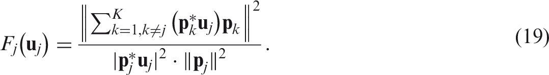
To evaluate the cost functions of equation (19), we need an initial set of source vector estimates ${\mathbf{p}}_j=a_j{\mathbf{g}}_j$ , which can be obtained with the standard CLEAN-SC method. Herein, the loop gain is set to 1, in order to obtain a unique marker location for each source. Then, updated marker locations can be obtained through successive minimisation of

$$\begin{array}{c}\multicolumn{1}{c}{F_j({\mathbf{u}}_j)=\frac{\Vert \sum _{k=1,k\ne j}^K{A}_k({\mathbf{g}}_k^{*}{\mathbf{u}}_j){\mathbf{g}}_k{\Vert }^2}{A_j^2|{\mathbf{g}}_j^{*}{\mathbf{u}}_j{|}^2·\Vert {\mathbf{g}}_j{\Vert }^2}.}\end{array}$$

(20)

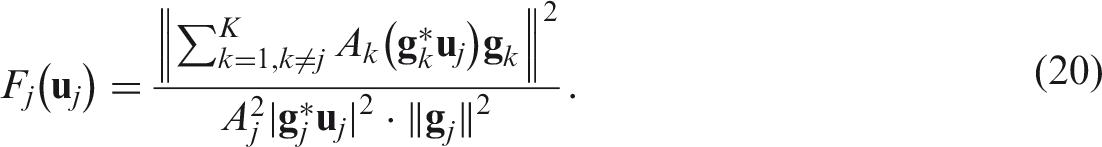
For each marker, the corresponding source component is

$${\mathbf{h}}_j=\frac{{\mathbf{Cu}}_j}{{\mathbf{u}}_j^{*}{\mathbf{Cu}}_j}.$$

(21)

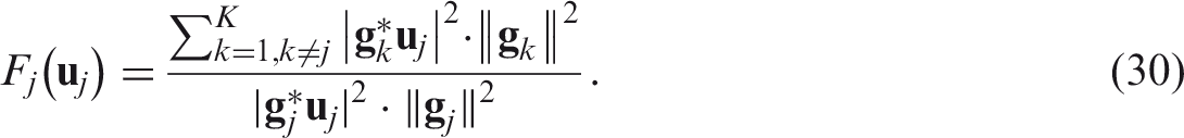
Source locations and power estimates are calculated by maximising the CB expression

$${\tilde{A}}_j={\mathbf{w}}_j^{*}{\mathbf{C}}_j{\mathbf{w}}_j,$$

(22)

where ${\mathbf{C}}_j$ is the CSM due to the j-th source, which can be written as

$${\mathbf{C}}_j\approx \alpha {\mathbf{h}}_j{\mathbf{h}}_j^{*},$$

(23)

for some constant α. This constant is obtained by inserting equation (21), yielding

$$\alpha ={\mathbf{u}}_j^{*}{\mathbf{C}}_j{\mathbf{u}}_j\approx {\mathbf{u}}_j^{*}{\mathbf{Cu}}_j.$$

(24)

The approximation herein is because ${\mathbf{u}}_j$ minimises equation (18). Thus, for the source power estimates, we have

$${\tilde{A}}_j=({\mathbf{u}}_j^{*}{\mathbf{Cu}}_j)|{\mathbf{w}}_j^{*}{\mathbf{h}}_j{|}^2.$$

(25)

After having performed these evaluations for each j, we can proceed with the next update by again successively minimising equation (20).

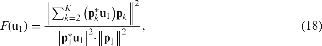
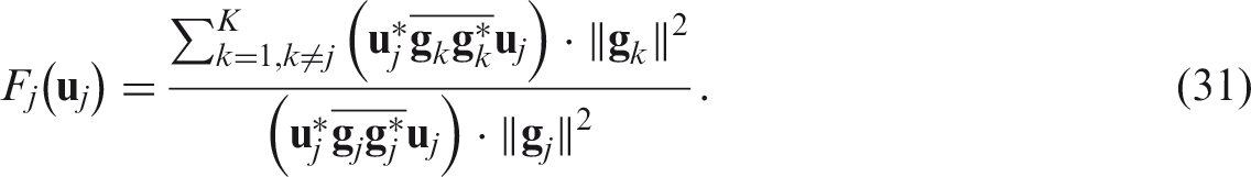
However, if sources of equal strength are spaced closely together (closer than the Rayleigh limit), then CLEAN-SC distributes the acoustic energy unequally over the source components. Thus, the weakest source contributes the least to the cost function, equation (20). This may lead to an optimum in which the weak sources remain weak. Therefore, we will omit the amplitudes in the cost function and use

$$F_j({\mathbf{u}}_j)=\frac{\Vert \sum _{k=1,k\ne j}^K({\mathbf{g}}_k^{*}{\mathbf{u}}_j){\mathbf{g}}_k{\Vert }^2}{|{\mathbf{g}}_j^{*}{\mathbf{u}}_j{|}^2·\Vert {\mathbf{g}}_j{\Vert }^2}.$$

(26)

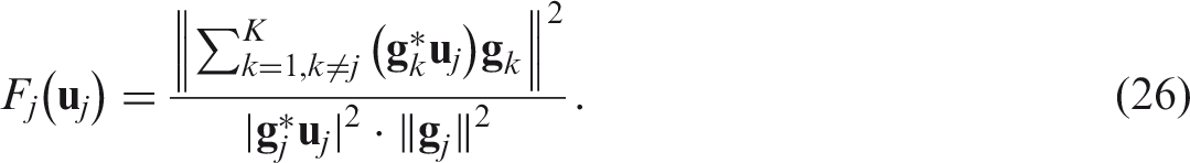
With this cost function, the solutions are basically scan grid points. This makes the solution space finite, so that the process can stop after a finite number of iterations.

To avoid division by zero in equation (26), we need to set a constraint on the marker location ${\mathbf{u}}_j$ :

$$|{\mathbf{g}}_j^{*}{\mathbf{u}}_j{|}^2\ge \mu >0.$$

(27)

This means that the PSF-value at the marker location is not more than $10\log (\mu )$ below the peak. Thus, if μ is larger than the largest side lobe level, the source marker will stay on the main lobe. In principle, the source marker could be located on a side lobe as well, but since beam patterns of actual sources may be different than the PSF, ⁷ it is safer to stay on the main lobe.

The method outlined above is called high-resolution CLEAN-SC (HR-CLEAN-SC), as it is a straightforward extension to standard CLEAN-SC, yielding a higher spatial resolution.

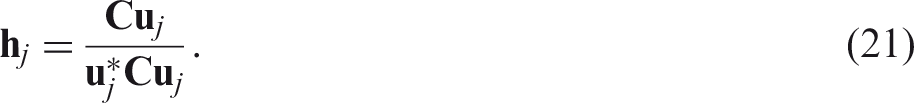
CSM diagonal removal

An important feature of CLEAN-SC is that it works well with CSM diagonal removal. In that case, the expression for the source component reads: ⁷

$${\mathbf{h}}_1=\frac{1}{1+{\mathbf{u}}_1^{*}{\mathbf{Hu}}_1}(\frac{{\overline{\mathbf{Cu}}}_1}{{\mathbf{u}}_1^{*}{\overline{\mathbf{Cu}}}_1}+{\mathbf{Hu}}_1),$$

(28)

in which the overbar in $\overline{\mathbf{C}}$ means ‘trimmed’, i.e. with the diagonal elements replaced by zeros. Further, H is a diagonal matrix, consisting of the diagonal elements of ${\mathbf{h}}_1{\mathbf{h}}_1^{*}$ . A solution of equation (28) is obtained by iteration. ⁷ The weight vector ${\mathbf{u}}_1$ is now calculated from the steering vector by ¹

$${\mathbf{u}}_1=\frac{{\mathbf{g}}_1}{(\Vert {\mathbf{g}}_1{\Vert }^4-\sum _{n=1}^N|g_{1,n}{|}^4{)}^{1/2}}.$$

(29)

There is no straightforward way to derive cost functions similar to equation (20) or (26). However, a reasonable estimate of equation (26) is

$$F_j({\mathbf{u}}_j)=\frac{\sum _{k=1,k\ne j}^K|{\mathbf{g}}_k^{*}{\mathbf{u}}_j{|}^2·\Vert {\mathbf{g}}_k{\Vert }^2}{|{\mathbf{g}}_j^{*}{\mathbf{u}}_j{|}^2·\Vert {\mathbf{g}}_j{\Vert }^2}.$$

(30)

The removed diagonal equivalent of equation (30) is

$$F_j({\mathbf{u}}_j)=\frac{\sum _{k=1,k\ne j}^K({\mathbf{u}}_j^{*}\overline{{\mathbf{g}}_k{\mathbf{g}}_k^{*}}{\mathbf{u}}_j)·\Vert {\mathbf{g}}_k{\Vert }^2}{({\mathbf{u}}_j^{*}\overline{{\mathbf{g}}_j{\mathbf{g}}_j^{*}}{\mathbf{u}}_j)·\Vert {\mathbf{g}}_j{\Vert }^2}.$$

(31)

The optimisation process is then equivalent to ‘High-resolution CLEAN-SC’ section. The source components ${\mathbf{h}}_j$ are calculated as in equation (28). Updated source locations are found by maximising the cost function G:

$$G({\mathbf{w}}_j)={\mathbf{w}}_j^{*}\overline{{\mathbf{h}}_j{\mathbf{h}}_j^{*}}{\mathbf{w}}_j$$

(32)

and source power estimates are calculated by

$${\tilde{A}}_j=({\mathbf{u}}_j^{*}{\overline{\mathbf{Cu}}}_j)({\mathbf{w}}_j^{*}\overline{{\mathbf{h}}_j{\mathbf{h}}_j^{*}}{\mathbf{w}}_j).$$

(33)

Simulated array data

In this section, we consider examples of 2D and 3D synthesised array measurements. The starting point for the simulations are CSMs obtained by evaluating summations like equation (1), so the assumptions listed in ‘The cross-spectral matrix (CSM)’ section are valid. By writing the CSM like this, separate sources are forced to be incoherent. For the threshold value introduced in equation (27), we choose:

$$\mu =0.25.$$

(34)

In other words, the PSF-value at the marker location is not more than 6 dB below the peak. As a rule, HR-CLEAN-SC needs not more than 10 iteration steps to converge to a solution of equation (26). However, in some cases, a repetitive loop exists between two solutions. Therefore, the maximum number of iterations was set to 20.

2D simulation

Array measurements were synthesised with a linear array of 2 m length, consisting of 101 microphones, uniformly spaced at 2 cm. The sound field consisted of plane waves, arriving from directions characterised by angles ${\theta }_k$ with respect to the y axis:

$$p_k(x,y)=a_k\exp \{\frac{2\pi \mathrm{if}}{c}[\cos ({\theta }_k)y+\sin ({\theta }_k)x]\}.$$

(35)

The array is on the $y=0$ line, so for the ‘measured’ pressures, we have

$$p_{k,n}=p_k(x_n,0)=a_k\exp \{\frac{2\pi \mathrm{if}}{c}\sin ({\theta }_k)x_n\}.$$

(36)

The simulated sound field consisted of two incoherent plane waves at 500 Hz, both at 1 Pa rms (94 dB), with incident angles −10° and −1°. Figure 2 shows the locations (angles) and the amplitudes of the sources, the CB array response, and the contributions from the sources individually (the PSFs). The angular spacing between the two sources is less than half the angular distance $\Delta \theta$ predicted by the Rayleigh criterion, which reads in two dimensions: ²

$$\Delta \theta =\frac{c}{\mathrm{Lf}},$$

(37)

where L is the length of the array. Therefore, CB is not able to resolve both sources, as is obvious from Figure 2. Consequently, CLEAN-SC cannot resolve the two sources either.

Figure 2.

Array response of sources at −10° and −1°, 500 Hz. Left: PSFs and ideal source marker locations; right: CLEAN-SC solution.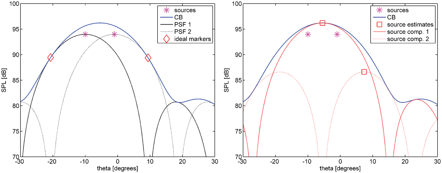

The HR-CLEAN-SC method, outlined in ‘High-resolution CLEAN-SC’ section, would give a perfect reconstruction of the PSFs if the source markers ${\mathbf{u}}_j$ would be at the locations where the PSF value of the other source is minimal. Those locations, which are indicated in Figure 2 (left), can only be determined if the PSFs and, hence, the source locations are known in advance, which is not always the case. However, we can iterate to the correct solution, as demonstrated in the following paragraphs.

The first step in the iteration process is made with standard CLEAN-SC. Herewith, two sources and corresponding source components are found as indicated in Figure 2 (right). The first source is found halfway the two actual sources and at a higher level. The second source has a much lower level and is found at a completely wrong location. However, this first estimate of the source locations is used to find first estimates of the source markers, by searching for minima of the PSFs associated with the source location estimates. The result is shown in Figure 3 (left).

Figure 3.

Sources at −10° and −1°, 500 Hz. Left: PSFs of CLEAN-SC solution and first marker estimates; right: first update of source estimates.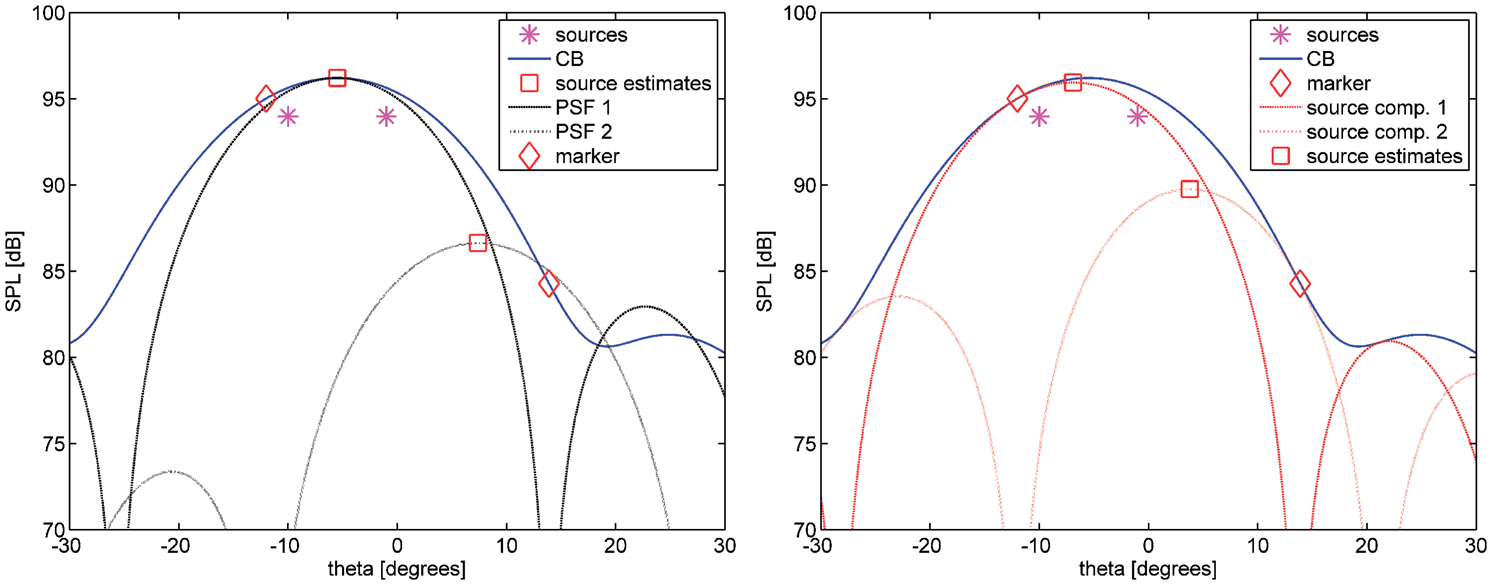

The next step is to calculate source components, equation (21), starting from these markers. Updated source locations are then found by searching the maximum value of the source components. This is illustrated in Figure 3 (right). By considering the PSFs of these updated source locations, we can find new marker locations, as illustrated in Figure 4 (left). With these new markers, we can determine new source components and update the source estimates, as shown in Figure 4 (right), and so on. By comparing the right-hand sides of Figures 2 to 4, we see that the source estimates clearly move into the directions of the true sources. After 10 iterations, the process has fully converged and the source estimates coincide with the true sources. This is shown in Figure 5.

Figure 4.

Sources at −10° and −1°, 500 Hz. Left: PSFs of first source updates and second marker estimates; right: second update of source estimates.

Figure 5.

Sources at −10° and −1°, 500 Hz. 10th update of source estimates.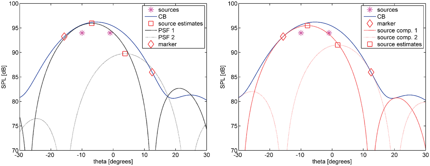

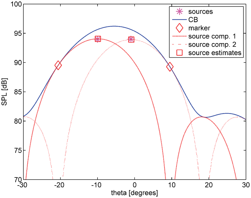
With this simulation, we demonstrated that the spatial resolution can be increased by a factor of 2 compared to the Rayleigh limit. The gain in resolution that can be attained depends on the constraint defined in equation (34). In fact, with the constraint value of 0.25 (6 dB), a gain by a factor 2.5 is possible in this 2D set-up (which follows from an analysis similar to the 3D analysis in Appendix 1).

Finally, it is noted that waves with equal strengths, as in this simulation, represent the worst case for HR-CLEAN-SC. When two sources have unequal strengths, the primary CB peak will be closer to the loudest source, and the associated CLEAN-SC source component contains less energy from the secondary source.

3D simulations

Simulations in three dimensions were made with an acoustic array in the $z=0$ plane. The array consisted of 133 microphones uniformly distributed over a disk with radius 0.6, as depicted in Figure 6. Acoustic fields of multiple incoherent point sources in the $z=1$ plane were simulated, each source at 94 dB. A series of six fixed frequencies were considered, ranging from 250 to 1500 Hz. The Rayleigh criterion ² for this set-up is approximately given by

$$\begin{array}{c}\multicolumn{1}{c}{\frac{\Delta x}{\Delta y}=1.218\frac{c}{\mathrm{Df}},}\end{array}$$

(38)

where D is the array diameter, $\Delta x$ the spacing between sources and $\Delta y$ the distance towards the array.

Figure 6.

Array for 3D simulations.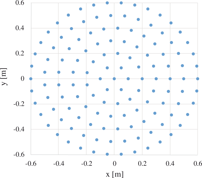

Two sources

The first simulation was made with two sources on the $x=0$ line, spaced 20 cm apart. The Rayleigh criterion, equation (38), predicts that sources can be separated at frequencies above 1700 Hz, hence for none of the frequencies considered in the simulation. This is confirmed by the CB-results (without CSM diagonal removal) in Figure 7 and the CLEAN-SC results in Figure 8. The intersections of the dashed lines indicate the locations of the sources.

Figure 7.

CB results with two sources (located at dashed line intersections).

Figure 8.

CLEAN-SC results with two sources (located at dashed line intersections).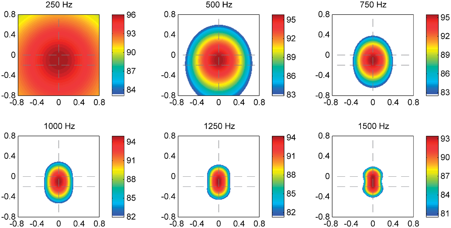

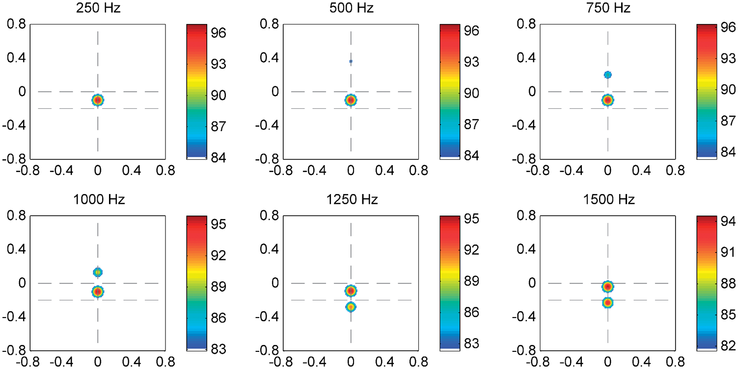
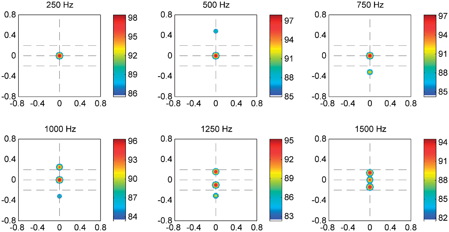
The HR-CLEAN-SC results are shown in Figure 9. A comparison with Figure 8 clearly shows the improvement of HR-CLEAN-SC, both in the location of the sources and in their estimated levels. The quality of the 500 Hz image in Figure 9 is comparable to the 1000 Hz image in Figure 8, and the same holds for the respective images at 750 Hz and 1500 Hz. Thus, it seems justified to conclude that the spatial resolution has increased by a factor 2. This is in line with the theory outlined in Appendix 1, where a gain by a factor 2.37 is predicted with $\mu =0.25$ .

Figure 9.

HR-CLEAN-SC results with two sources (located at dashed line intersections).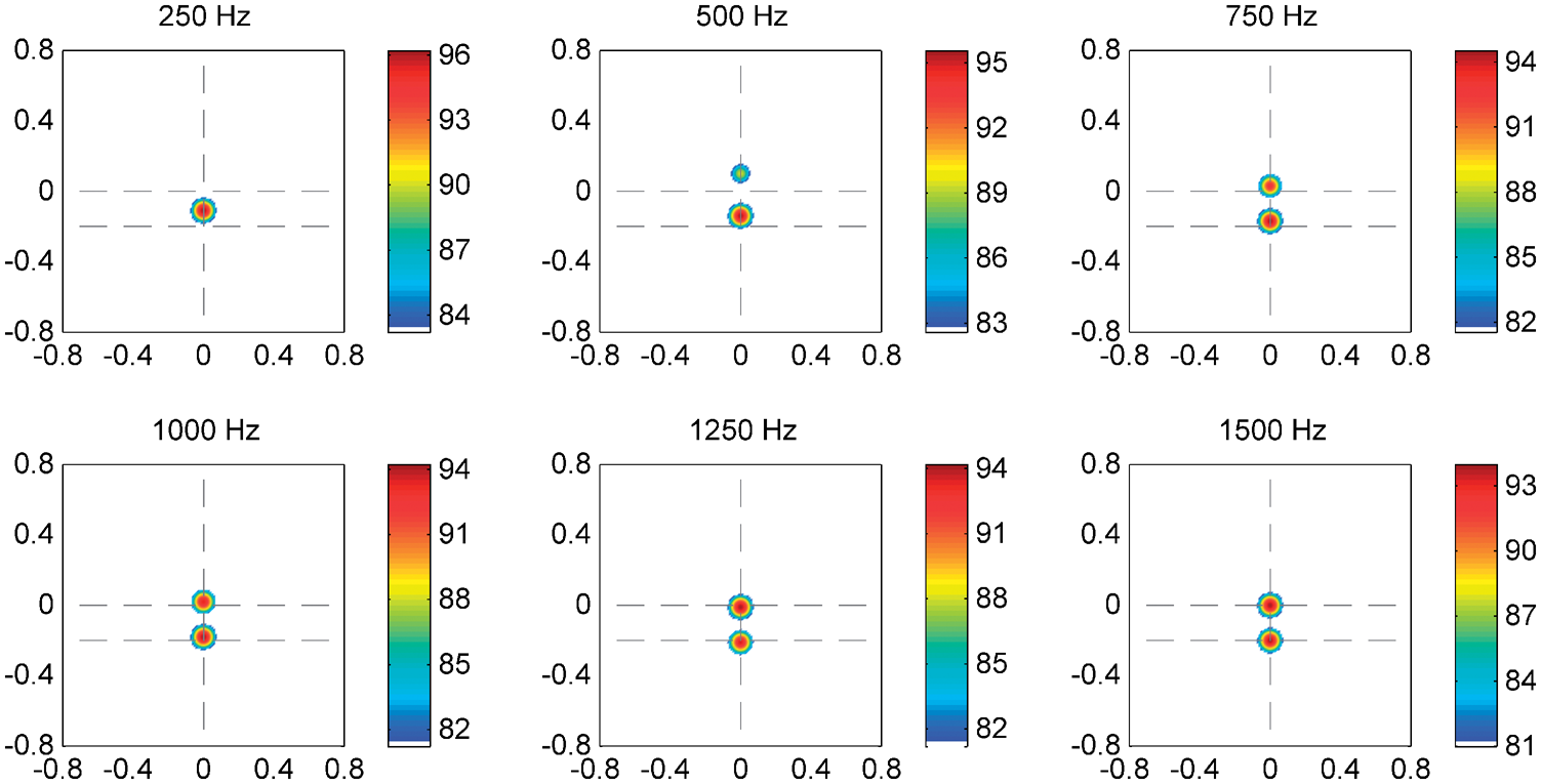

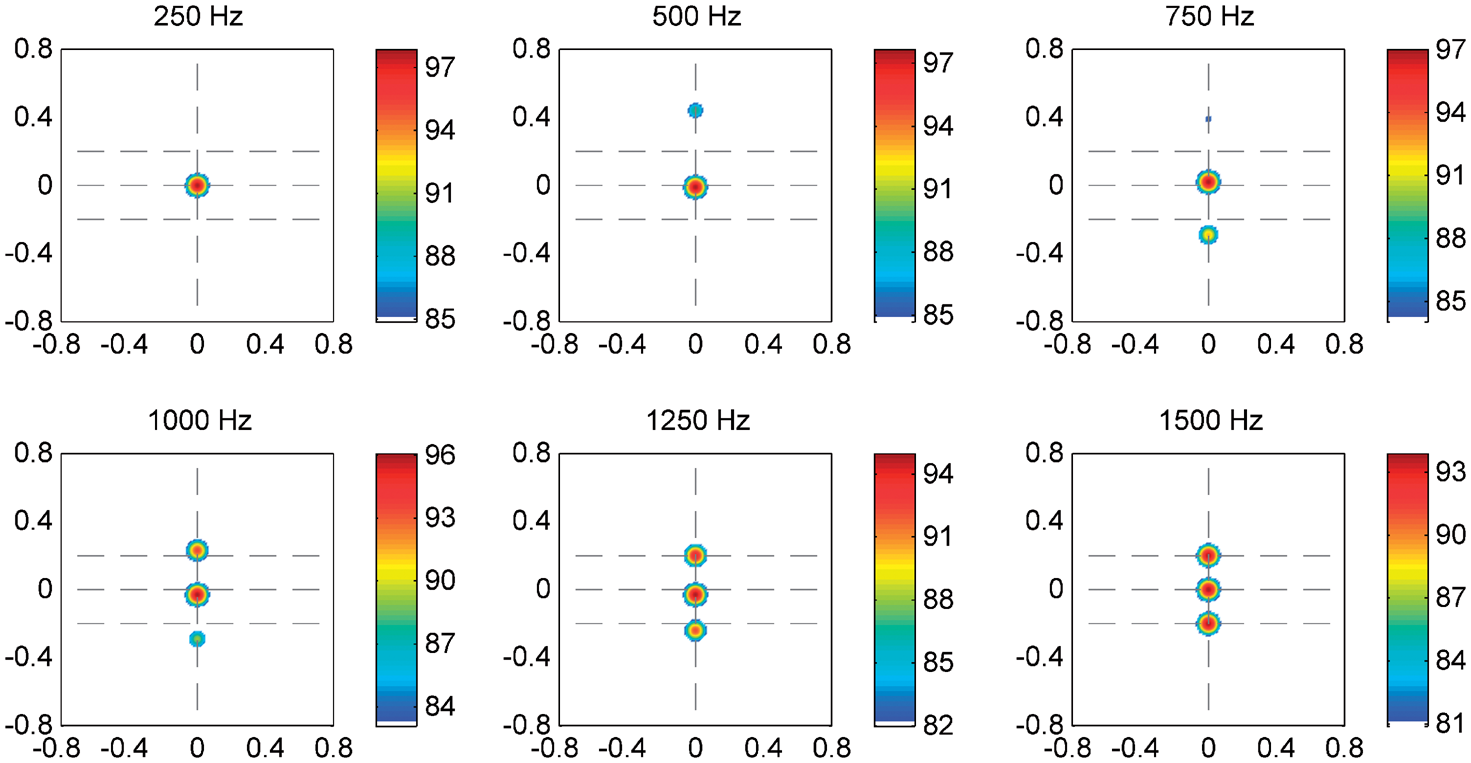
The beamform images in Figures 7 to 9 were obtained with the full CSM. However, in many beamforming applications, it is necessary to remove the diagonal. As outlined in ‘CSM diagonal removal’ section, the HR-CLEAN-SC approach without the CSM diagonal is less exact. This is confirmed by Figure 10, which is the removed diagonal equivalent of Figure 9. The results without diagonal are a little worse (especially at the lower part of the frequency range) than with full CSM. Nevertheless, there is still significant improvement compared to standard CLEAN-SC.

Figure 10.

HR-CLEAN-SC results with two sources (located at dashed line intersections); CSM diagonal removed.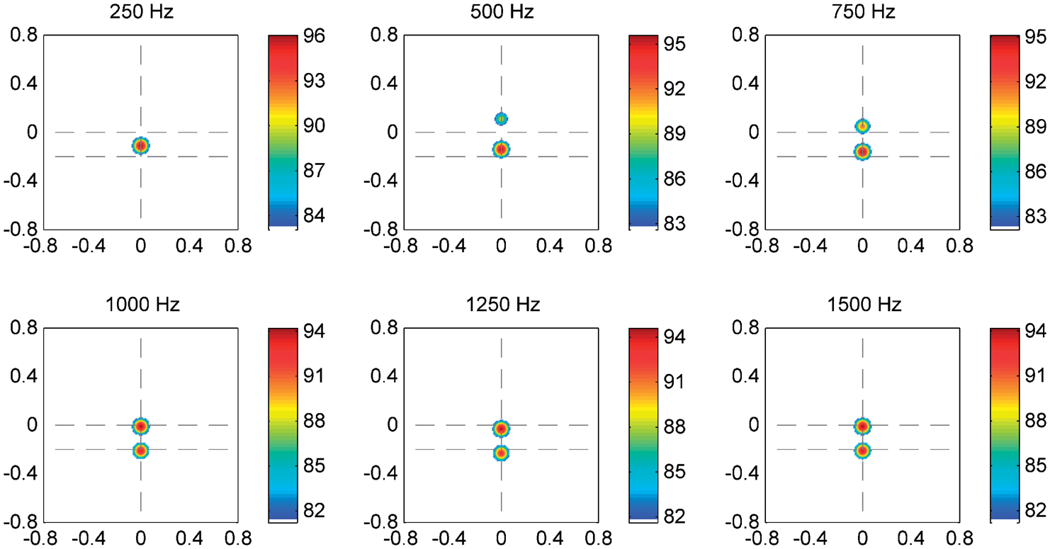

In the remaining part of this article, we consider beamforming only with the full CSM.

More than two sources

When the HR-CLEAN-SC method is applied to more than two sources, the summation in the numerator of equation (26) is done for more than one steering vector ${\mathbf{g}}_k$ . Thus, there is less freedom in minimising equation (26). Consequently, the improvements obtained with HR-CLEAN-SC are expected to be smaller than with two sources.

First, a simulation was made with three sources, again on the $x=0$ line and with 20 cm spacing. The CB-results are shown in Figure 11, the CLEAN-SC results in Figure 12, and the HR-CLEAN-SC results in Figure 13. The HR-CLEAN-SC results are still significantly better than the standard CLEAN-SC results, but the resolution improvement is no longer by a factor of 2.

Figure 11.

CB results with three sources (located at dashed line intersections).

Figure 12.

CLEAN-SC results with three sources (located at dashed line intersections).

Figure 13.

HR-CLEAN-SC results with three sources (located at dashed line intersections).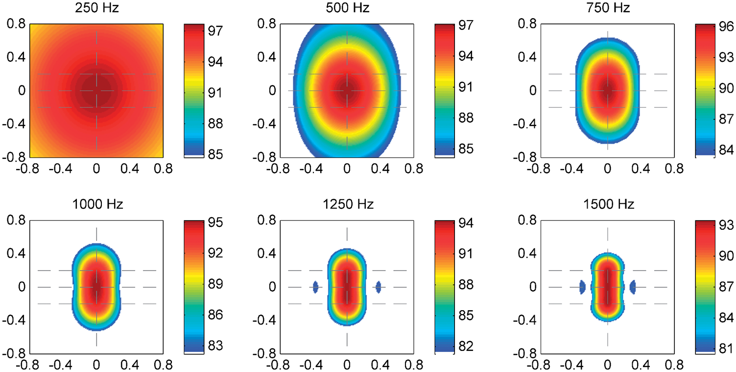

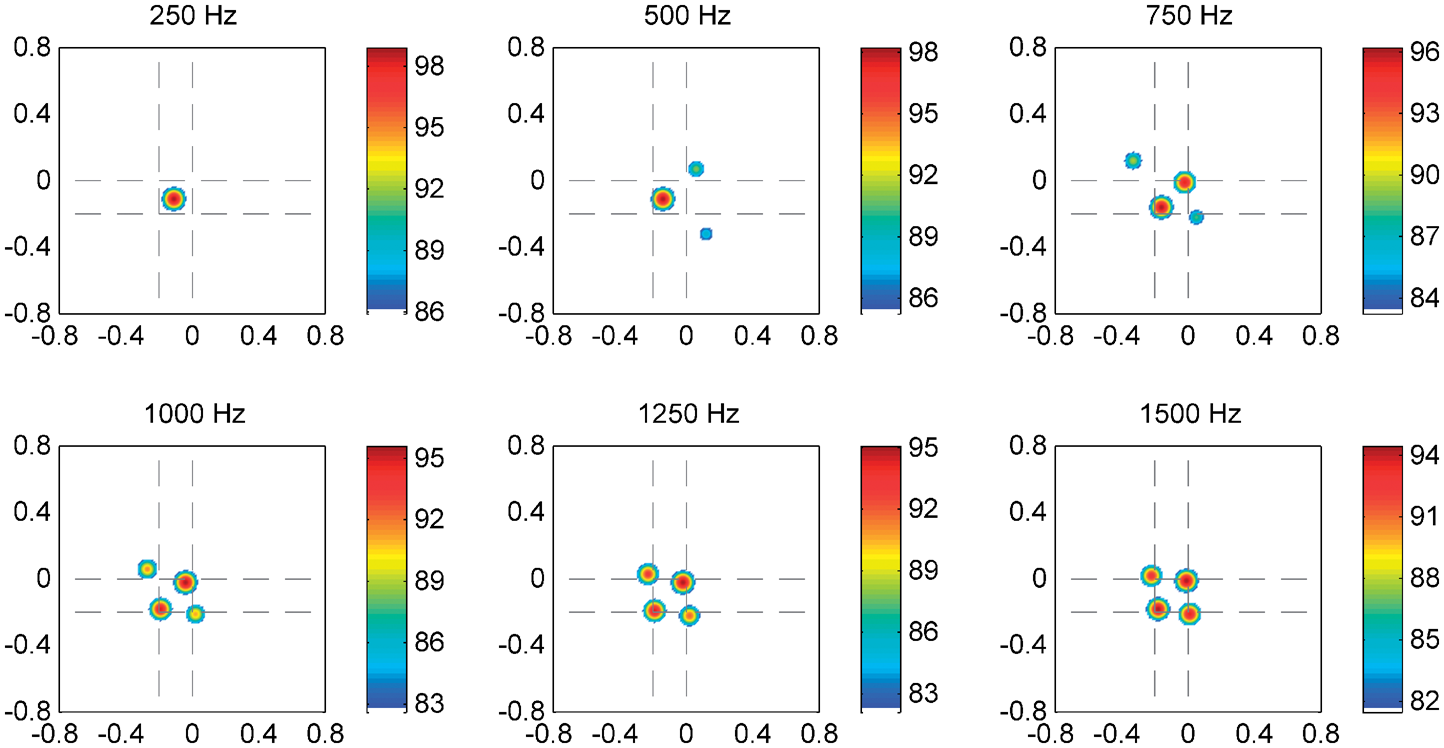
The trend of reduced added value is continued when four sources are closely spaced. This can be concluded from beamforming simulations shown in Figures 14 (CB), 15 (CLEAN-SC) and 16 (HR-CLEAN-SC).

Figure 14.

CB results with four sources (located at dashed line intersections).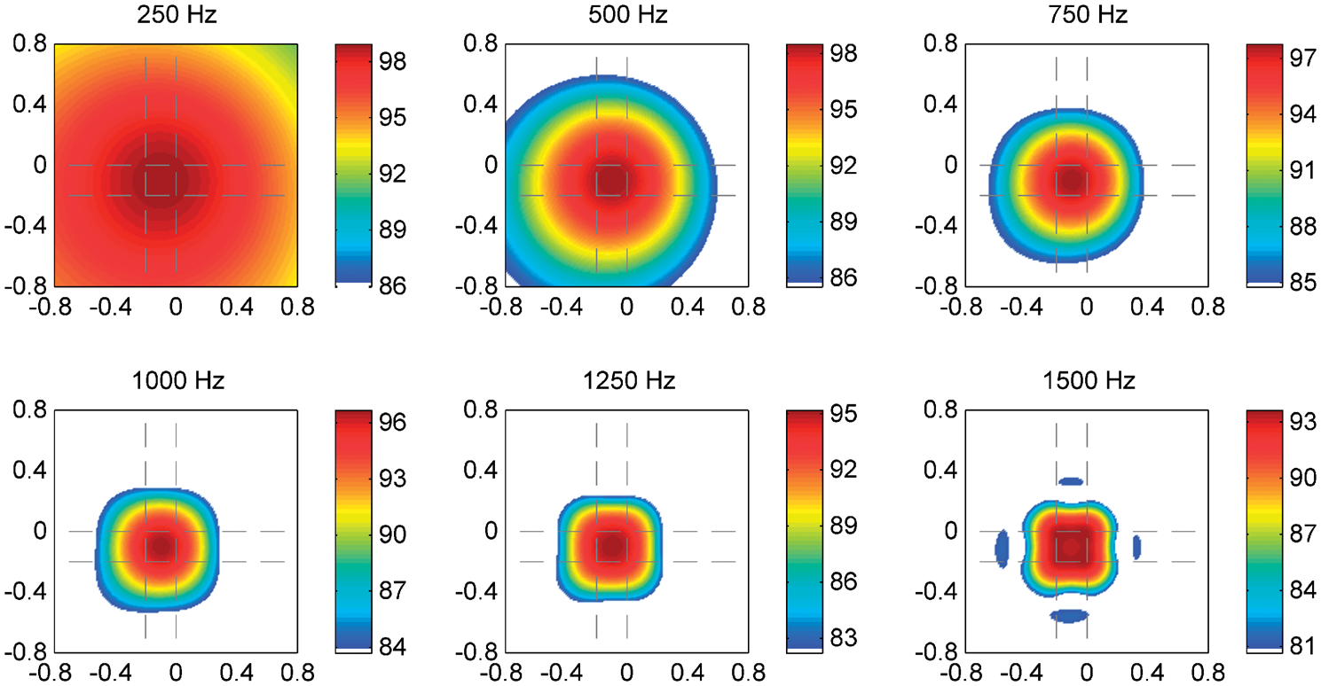

Experimental validation

Set-up

An experiment was performed in the anechoic chamber at the Faculty of Applied Sciences of Delft University of Technology (TU Delft). A 56-microphone array with a random distribution and a diameter of approximately 1 m was employed (see Figure 17). The microphones in the array are surrounded by a layer of absorption foam called ‘Flamex basic’, 15 mm thick. This avoids diffraction to a certain extent, especially for acoustic waves coming from directions close to normal, such as in this experiment. The array plane formed an angle of 4° with the vertical, which was accounted for in the microphone positions.

Figure 15.

CLEAN-SC results with four sources (located at dashed line intersections).

Figure 16.

HR-CLEAN-SC results with four sources (located at dashed line intersections).

Figure 17.

Set-up in TU Delft anechoic chamber with array of 56 microphones and two speakers.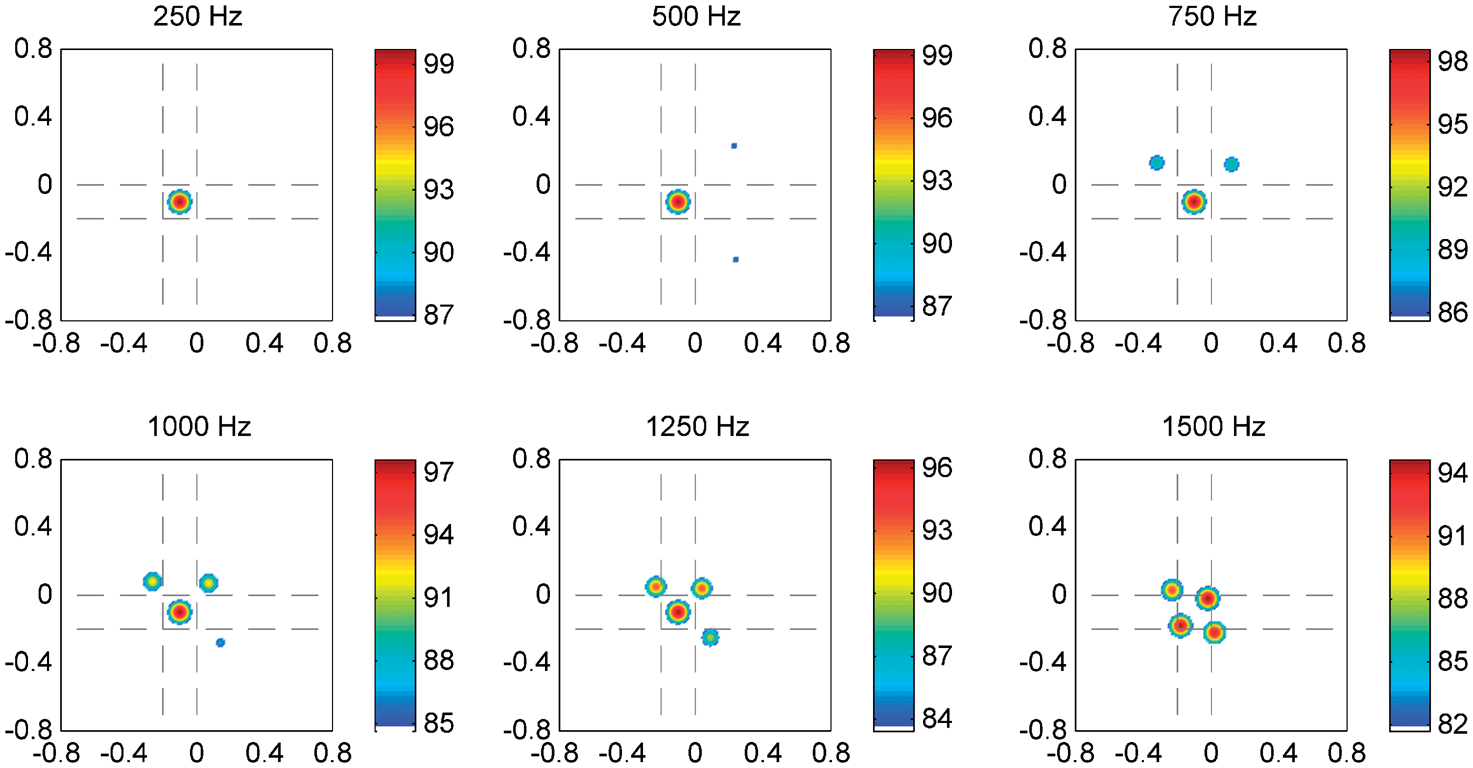

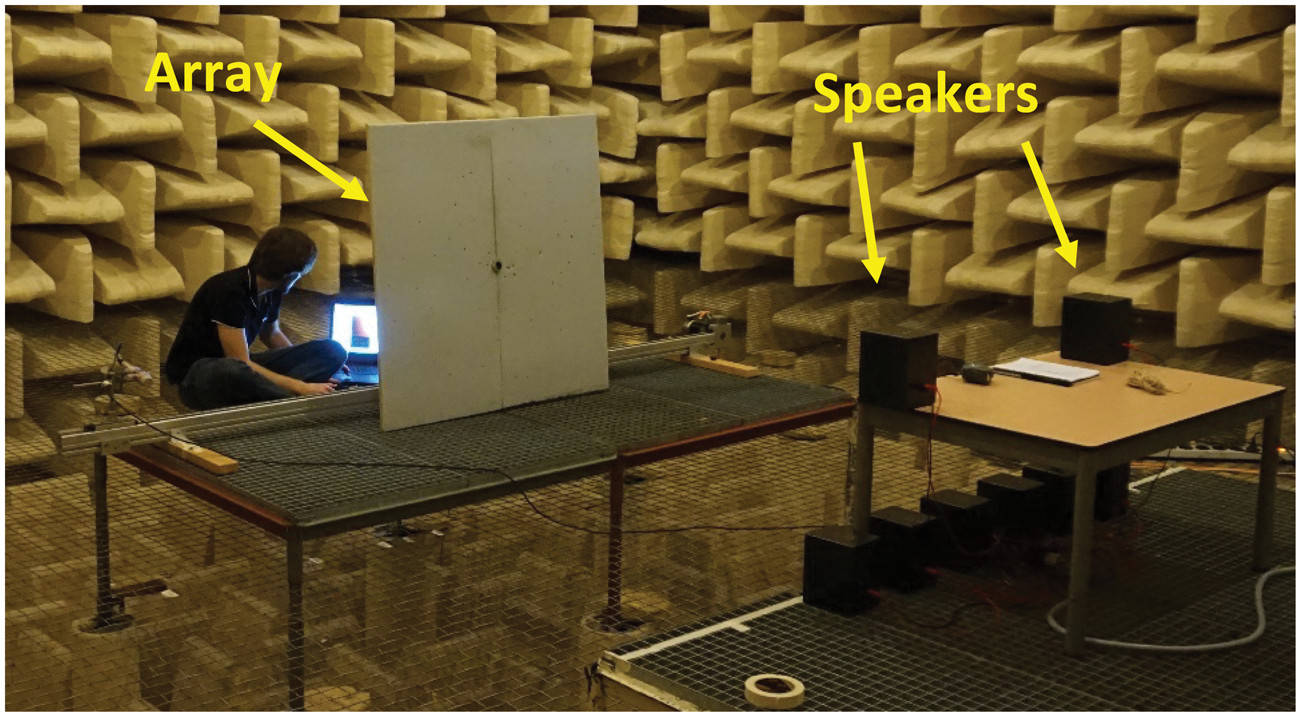
Two small speakers were located at 1.87 m from the array, at a number of different distances between each other: 12 cm, 25 cm, 50 cm and 80 cm. The speakers were placed on the table, with their baffles as far away from the table edge as possible, to avoid reflections. Tests performed with a sound level meter with and without table showed negligible differences in the sound levels measured. Thus, the influence of the table presence could be assumed negligible.

The two speakers were incoherently fed with white noise at 50 kHz sampling frequency. At each mutual speaker distance, three measurements were performed: (a) with both speakers active, (b) with only the left speaker on and (c) with only the right speaker on. When one of the speakers was turned off, the other was fed with (statistically) the same white noise signal as with both speakers on, so that beamforming results with both speakers could be compared against single speaker measurements. The recording time per measurement was 30 s, using a 50 kHz sampling frequency.

To obtain the time-averaged CSM, the acoustic data were separated into time blocks of 500 samples, yielding a frequency resolution of 100 Hz. FFT was applied with Hanning window and 50% overlap.

Results

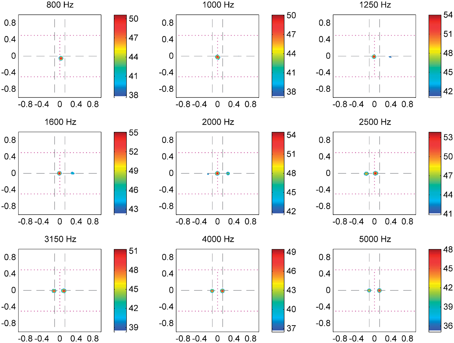
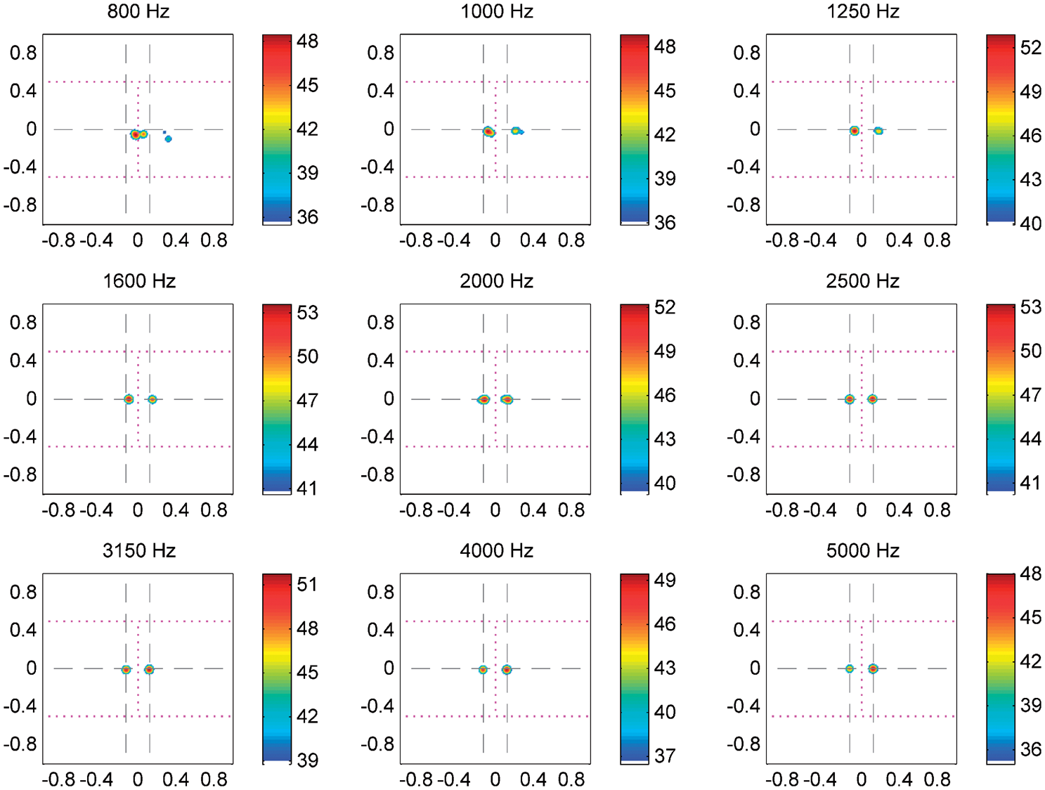
Beamforming (CB, CLEAN-SC and HR-CLEAN-SC) was applied at each narrowband frequency up to 10 kHz, and then summed up to 1/3 octave bands. HR-CLEAN-SC was applied under the same conditions as with the simulated data, mentioned in the first part of ‘Simulated array data’ section. Results with the two speakers at 25 cm separation distance are shown in Figures 18 to 20. At 25 cm separation, the Rayleigh criterion, equation (38), predicts resolvability at frequencies above 3000 Hz. This is confirmed by the CB and the CLEAN-SC results, shown in Figures 18 and 19, respectively. The HR-CLEAN-SC images in Figure 20 show significant resolution improvements at 1/3 octave band frequencies ranging from 1000 to 2500 Hz, so at frequencies considerably below the Rayleigh frequency limit. Just as for the simulations reported in ‘3D simulations’ section, a factor 2 is found for the resolution improvement, which agrees with the theoretical gain factor of 2.37, derived in Appendix 1.

Figure 18.

CB results with two sources in anechoic chamber, at 25 cm distance; sources located at dashed line intersections; dotted lines indicate integration areas.

Figure 19.

CLEAN-SC results with two sources in anechoic chamber, at 25 cm distance; sources located at dashed line intersections; dotted lines indicate integration areas.

Figure 20.

HR-CLEAN-SC results with two sources in anechoic chamber, at 25 cm distance; sources located at dashed line intersections; dotted lines indicate integration areas.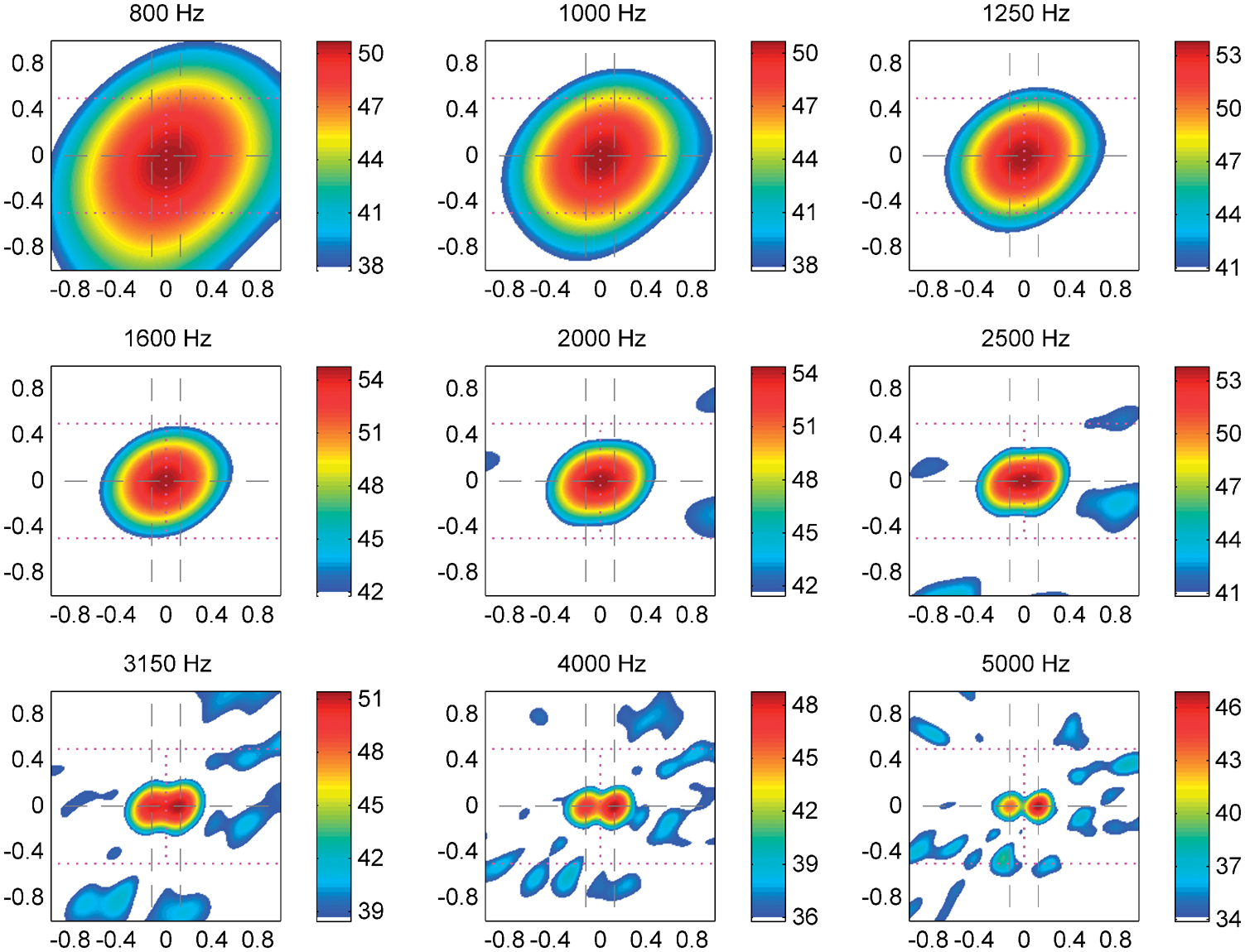

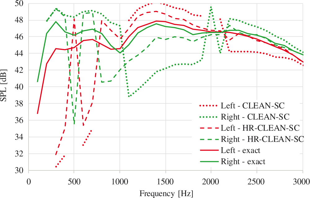
CLEAN-SC integration ⁷ was performed on the areas within the dotted lines in Figures 18 to 20. Integrated data obtained with CLEAN-SC and HR-CLEAN-SC with both loudspeakers on were compared against single speaker integrated results, which is shown in Figure 21. ^a The improvement obtained with HR-CLEAN-SC is clearly visible, especially between 1000 and 3000 Hz. See also the zoomed plot, Figure 22. However, the factor 2 is not entirely confirmed: the HR-CLEAN-SC results at 1500 Hz are worse than the CLEAN-SC results at 3000 Hz. Note that HR-CLEAN-SC also outperforms standard CLEAN-SC at high frequencies, thanks to the freedom in choosing the marker locations.

Figure 21.

CLEAN-SC and HR-CLEAN-SC integrated results with two sources in anechoic chamber, at 25 cm distance, compared against ‘exact’ single speaker measurements.

Figure 22.

Zoomed version of Figure 21.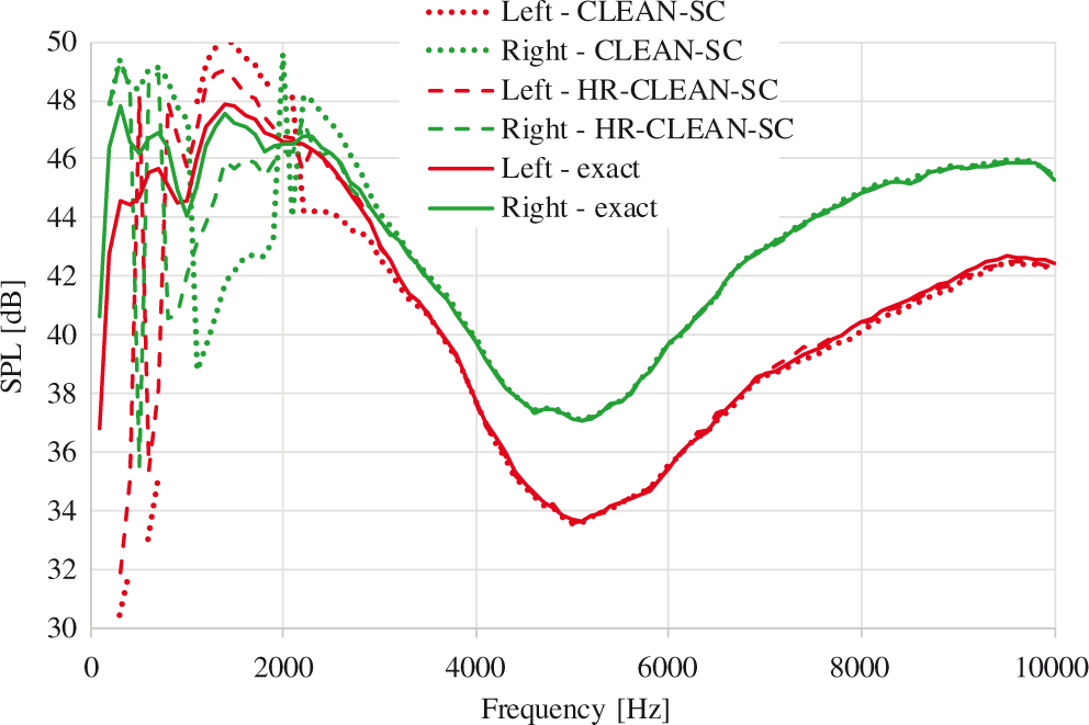

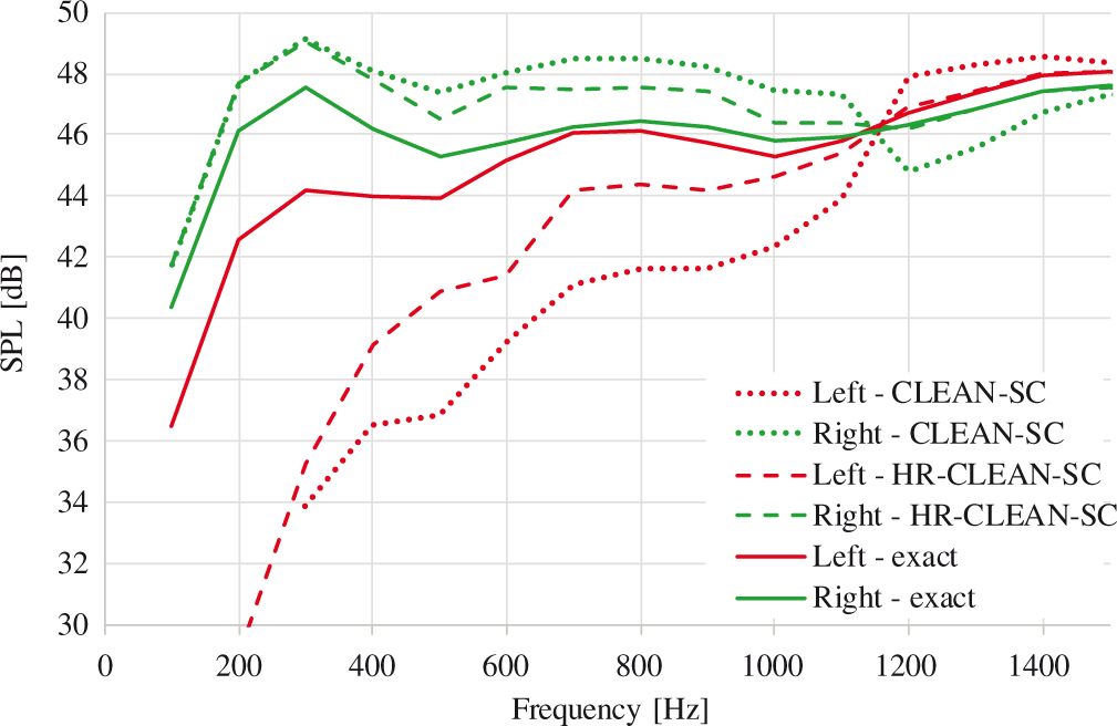
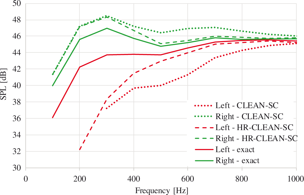
Similar results were found at other speaker distances. The results are summarised in Figures 23 (12 cm), 24 (50 cm) and 25 (80 cm). Each plot has its own range of frequencies. Note that there is always a trade-off in the spectra: if the right speaker level is underpredicted, then the left speaker level is overpredicted and vice versa. The total level is predicted correctly.

Figure 23.

CLEAN-SC and HR-CLEAN-SC integrated results with two sources in anechoic chamber, at 12 cm distance, compared against ‘exact’ single speaker measurements.

Figure 24.

CLEAN-SC and HR-CLEAN-SC integrated results with two sources in anechoic chamber, at 50 cm distance, compared against ‘exact’ single speaker measurements.

Figure 25.

CLEAN-SC and HR-CLEAN-SC integrated results with two sources in anechoic chamber, at 80 cm distance, compared against ‘exact’ single speaker measurements.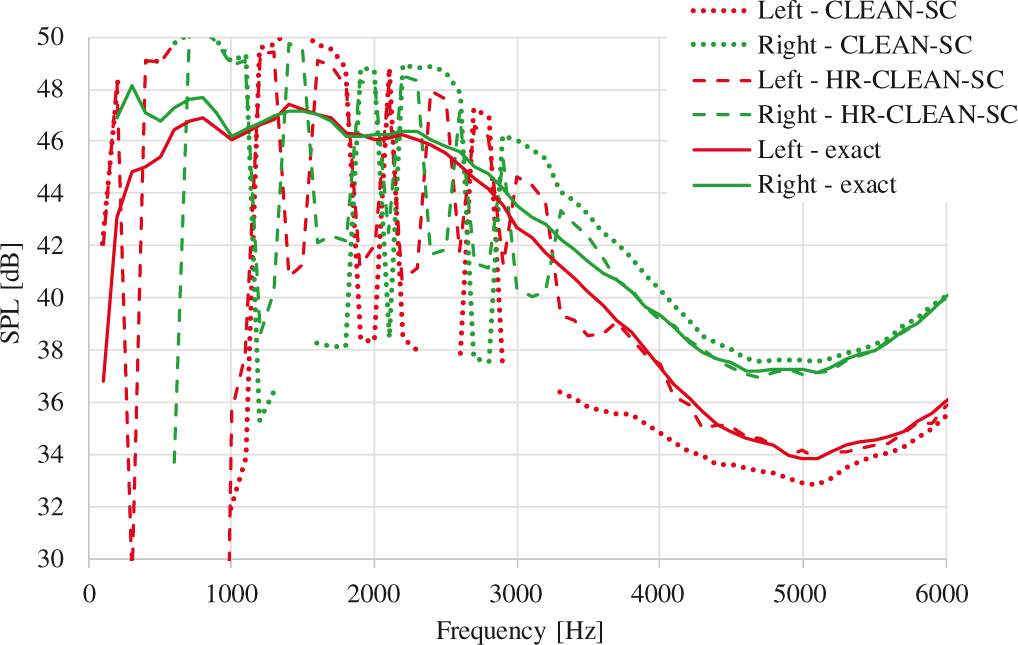

Conclusions

The HR-CLEAN-SC method, proposed in this article, is a high-resolution extension of CLEAN-SC. It is particularly suitable for pairs of closely spaced sources. Then the spatial resolution can be increased by, typically, a factor of 2. The features of the standard CLEAN-SC method are fully preserved. For beamforming applications with many sources (e.g. airframe noise measurements in wind tunnels), HR-CLEAN-SC is not expected to give much added value.

Obviously, HR-CLEAN-SC needs more computation time than CLEAN-SC. However, the most time-consuming part, which is CB at the start of the iteration process, does not need to be done more often. Consequently, when only a few CLEAN-SC iterations are needed, i.e. when the number of sources K is small, the additional computation time is limited.

HR-CLEAN-SC can be applied with and without removal of the CSM diagonal. In both cases, significant increase in resolution is found compared to the standard CLEAN-SC method. Without CSM removal, i.e. with the full CSM, the best results are obtained. When it is necessary to remove the diagonal, HR-CLEAN-SC may benefit from reconstruction methods. ¹⁰

The features of HR-CLEAN-SC were demonstrated with synthesised 2D and 3D array measurements. Experimental validation was done by measurements with two loudspeakers in an anechoic chamber.