Simulating isothermal Euler model with non-vacuum initial data via mR scheme

Abstract

We consider the isothermal Euler model with non-vacuum initial data. We extract the Riemann invariants of the isothermal Euler model, which admits vital applications. We also design the modified Rusanov (mR) scheme to solve the isothermal Euler model. This scheme consists of two steps, the first step of the scheme depends on a local parameter allowing to control diffusion. The second stage recovers conservation equation. This technique is a straightforward to implement and precise. We compare this scheme with the Rusanov scheme via three numerical examples. This numerical study verifies the efficiency of the mR scheme. Finally, the mR scheme can be used to solve many other models in applied science.

Introduction

The nonlinear hyperbolic systems of conservation laws take the form

$$U_t+F{\left(U\right)}_x=0.$$

(1)

These equations allow shocks and rarefaction wave solutions. A comprehensive survey on hyperbolic conservation laws and their applications can be found, for instance, the monographs of Majda ¹ Godlewski and Raviart, ² Glimm, ³ Evans, ⁴ Dafermos, ⁵ Smoller, ⁶ and LeVeque.^7,8 Indeed the solutions for the general initial value problems of hyperbolic conservation laws admit very vital features in applied science, such as the ultra-relativistic Euler equations,^9,10 the shallow water equations, ¹¹ and the phonon-Bose model. ¹² Behind several mathematical models, actually there is the very important “conservation law,” ^{13, 14} . In particular, equation (1) is a particular conservation law, where essentially a precise flux is fixed. Exactly by changing accordingly to the model the expression of the flux, equation (1) can read in other ways; in particular, it can become also a second-order PDE (partial differential equation) with diffusion and sources. In this sense, Keller–Segel problems from mathematical biology may involve nonlinear diffusion and external actions. Moreover, there are recent development in numerical techniques for solving various models arising in applied sciences and engineering, such as Volterra integro-differential equations of pantograph-delay type, ¹⁵ Telegraph equations, ¹⁶ linear complex differential equations, ¹⁷ systems of high-order Fredholm integro-differential equations,^18,19 nonlinear fractional Volterra integro-differential equations, ²⁰ systems of high-order linear differential–difference equations, ²¹ system of linear Volterra integral equations with variable coefficients, ²² second-order hyperbolic partial differential equation, ²³ nonlinear stochastic Itô-Volterra integral equations, ²⁴ and nonlocal reaction chemotaxis model. ²⁵

One of the most important models in fluid dynamics is the Euler equations, which are a set of quasilinear PDE equations governing adiabatic and inviscid flow. The linearized Euler equations are derived from Euler’s equations, with no thermal conduction and no viscous losses. The fluid in the linearized Euler physics interface is assumed to be an ideal gas. Indeed, a linearized Euler equation method is developed to investigate the choked combustor. ²⁶

In this paper, we consider the isothermal Euler model, which given as follows

$$\begin{array}{l}{\left(\rho \right)}_t+{\left(\rho v\right)}_x=0,\hfill \\ {\left(\rho v\right)}_t+{\left(\rho v^2+p\right)}_x=0,\hfill \end{array}$$

(2)

$\rho =\rho \left(t,x\right):\left[0,\infty \right)\times ℝ\to \left(0,\infty \right)$ and $v=v\left(t,x\right):\left[0,\infty \right)\times ℝ\to ℝ$ denote the density and the velocity resp. Indeed, p represents pressure and the equation of state is

$$p=p\left(\rho \right)=c^2\rho ,$$

(3)

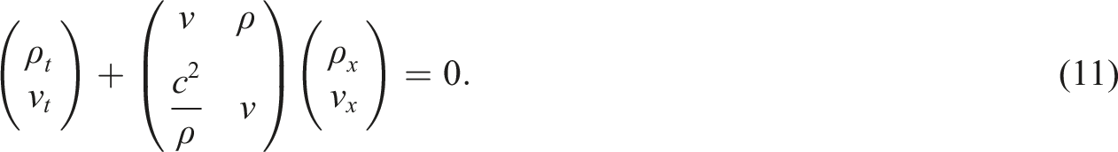
c is a non-zero constant propagation speed of sound. Sometimes one also refers this as pressure law. The isothermal equations become

$$\begin{array}{l}{\left(\rho \right)}_t+{\left(\rho v\right)}_x=0,\hfill \\ {\left(\rho v\right)}_t+{\left(\rho v^2+c^2\rho \right)}_x=0.\hfill \end{array}$$

(4)

Equation (4) models the flow of gas at constant temperature and flow of fluids for pressure ranges. The physical fields are supposed to rely on time $t\in {ℝ}_{t\ge 0}$ ; space $x\in ℝ$ , ^{27, 28} . In fact, this model has so many interesting applications in fluid dynamics and physics. Marchesin and Paes-Leme ²⁷ investigated the Riemann problem of model equation (4) in a duct with discontinuous cross-sectional area by attaching the stationary wave curve to the first and third wave curves. LeFloch and Shelukhin ²⁹ used the symmetry and scaling properties of both the isothermal Euler equations and the entropy-wave equation. Chen and Wang investigated the Cauchy problem for the Euler equations for compressible fluids. ³⁰ In the operation of the gas pipelines, there are strict upper bounds for the velocities in order to avert noise pollution by pipeline vibrations, which can be generated by the flow.^31,32 For further details concerning the isothermal Euler model, we refer to^33,34 and references therein.

In the case of a non-vacuum initial data, density stays positive for t ≥ 0. First equation of model equation (4) shows that the ρ(t, x) is determined by ρ₀(x) and an exponential function through a characteristic curve.

Lemma 1.1

If ρ₀(x) > 0 for all $x\in {ℝ}^N$ , then ρ(t, x) > 0 ∀ t ≥ 0 and $\forall x\in {ℝ}^N$ . ³⁵

Here the numerical mR scheme is used to solve one-dimensional isothermal Euler equations of gas dynamics. Actually, the Rusanov’s method is a local Lax–Friedrichs method that one seeks a local maximum rather than a global maximum of the wave speed, which is illustrated. ³⁶ In the proposed scheme in this paper, we used the local Rusanov velocity for extension in two dimensions because the calculation of Rusanov velocity is very easy with respect to the mesh Δ x with triangular mashes. The mR scheme has been implemented to solve a scalar conservation laws with stochastic time-space dependent flux function ³⁷ and non-homogeneous systems of conservation laws.^38,39 The mR technique has many advantages. First, it can compute the numerical flux corresponding to the real state of solution in the absence of Riemann problem solvers. Second, reasonable accuracy can be obtained easily and no special treatment is needed for the numerical solution of the isothermal Euler model with non-vacuum initial data because it is performed automatically in the integrated numerical flux function. Third, it is easy to implement, it is accurate, and moreover it avoids the solution of Riemann problems during the time integration process. On the other hand, the first stage (predictor) of the scheme depends on a local parameter allowing us to control diffusion, which modulates by using the limiters theory and Riemann invariant. In some models, the computation of Riemann invariant is so difficult, which is considered the only weakness point of this method. The mR scheme is linearly stable provided the condition for the canonical Courant–Friedrichs–Lewy (CFL) is satisfied. Moreover, this scheme is robust and efficient tool for solving many other hyperbolic systems of conservation laws, like the Ripa model, ⁴⁰ the blood flow in human artery, ⁴¹ and the Chaplygin gas model. ⁴² Actually, the presented results can be described the isothermal Euler equations with phase transition between a liquid and a vapor phase. ⁴³

We write equation (4) in a conserved form

$$U_t+F{\left(U\right)}_x=0,$$

(5)

$$U=\left(\begin{array}{c}{U}_1\\ U_2\end{array}\right)=\left(\begin{array}{c}\rho \\ \rho v\end{array}\right), F\left(U\right)=\left(\begin{array}{c}\rho v\\ \rho v^2+c^2\rho \end{array}\right).$$

(6)

The domains Λ, Ω of the (ρ, v), and (U₁, U₂) state spaces are

$$\begin{array}{l}\mathrm{\Lambda }=\left\{\left(\rho ,v\right)\in {ℝ}^{+}\times ℝ\right\},\hfill \\ \mathrm{\Omega }=\left\{\left(U_1,U_2\right)\in {ℝ}^{+}\times ℝ\right\},\hfill \end{array}$$

(7)

respectively.

Proposition 1.1

The mapping ϒ : Λ → Ω

$$\mathrm{{\rm Y}}\left(\rho ,v\right)=\left(\begin{array}{c}\rho \\ \rho v\end{array}\right)$$

(8)

is 1-1. Indeed, the corresponding Jacobian determinant is continuous and not equal zero.

Proof. First, we show that the mapping is injective. Let (ρ₁, v₁), (ρ₂, v₂) ∈ Λ with U₁(ρ₁, v₁) = U₁(ρ₂, v₂), U₂(ρ₁, v₁) = U₂(ρ₂, v₂). First, we have that v₁ = v₂ then ρ₁ = ρ₂. Second, we prove that this mapping is surjective: For each (U₁, U₂) ∈ Ω, there is

$$\left({\rho }_1,v_1\right)=\left(U_1,\frac{U_2}{U_1}\right)\in \mathrm{\Lambda },$$

(9)

such that

$$\mathrm{\Upsilon }\left({\rho }_1,v_1\right)=\left(\begin{array}{c}{U}_1\\ U_2\end{array}\right).$$

(10)

A simple computation yields

$$\mathit{det}\left(\frac{\partial (\left(U_1,U_2\right)}{\partial \left(\rho ,v\right)}\right)=\rho ,$$

this completes the proof.

We put the equation (4) in the quasilinear form

$$\left(\begin{array}{c}{\rho }_t\\ v_t\end{array}\right)+\left(\begin{array}{cc}v& \rho \\ \frac{c^2}{\rho }& v\end{array}\right)\left(\begin{array}{c}{\rho }_x\\ v_x\end{array}\right)=0.$$

(11)

The characteristic velocities (eigenvalues) for equation (4) are

$${\mu }_1=v-c<{\mu }_2=v+c,$$

(12)

c is the sound speed, which is corresponding to the 1 and 2 family of waves, respectively.

The eigenvectors for equation (4) are

$$r_1={\left(-\frac{\rho }{c},1\right)}^T,r_2={\left(\frac{\rho }{c},1\right)}^T.$$

(13)

Proposition 1.2

System equation (4) is strictly hyperbolic and genuinely nonlinear for ρ > 0 and $v\in ℝ$ .

Proof. The system equation (4) is strictly hyperbolic, since

$${\mu }_2-{\mu }_1=2c>0.$$

(14)

Indeed

$$\nabla {\mu }_1·r_1=\nabla {\mu }_2·r_2=1 > 0,$$

(15)

which admits the genuine nonlinearity.

For the details about the parametrization of shock waves and rarefaction waves, we refer to.[28,43]

The structure of this article is given as follows. The Riemann invariants of the isothermal Euler model equation (4) are formulated in Riemann Invariants. In Modified Rusanov scheme, we design the proposed scheme to solve the 1-D isothermal Euler equations. The numerical applications, numerical results, and comparison with the Rusanov scheme and HLL scheme are given in Numerical Results. Conclusion is drawn in Conclusions.

Riemann invariants

The Riemann invariants admit various interesting applications in different fields of applied science.^11,28 We deduce these invariants for isothermal Euler model equation (4).

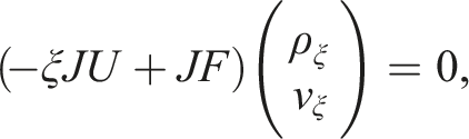
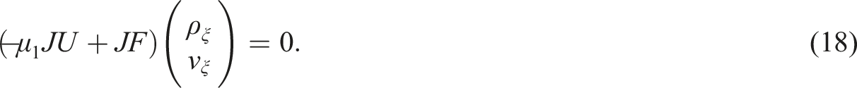
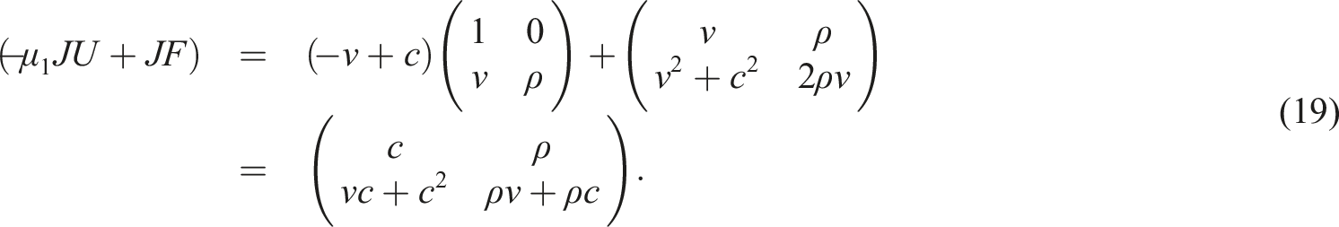
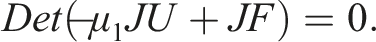
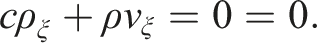
Assuming that eigenvalue $\xi =\frac{x}{t}$ , then $U=U\left(\frac{x}{t}\right)$ satisfies

$$\left(-\xi JU+JF\right)\left(\begin{array}{c}{\rho }_{\xi }\\ v_{\xi }\end{array}\right)=0,$$

where

$$U=\left(\begin{array}{c}\rho \\ \rho v\end{array}\right),F\left(U\right)=\left(\begin{array}{c}\rho v\\ \rho v^2+c^2\rho \end{array}\right)$$

(16)

and

$$JU=\left(\begin{array}{cc}1& 0\\ v& \rho \end{array}\right),JF=\left(\begin{array}{cc}v& \rho \\ v^2+c^2& 2\rho v\end{array}\right).$$

(17)

If $\left(\begin{array}{c}{\rho }_{\xi }\\ v_{\xi }\end{array}\right)\ne 0$ , then $\left(\begin{array}{c}{\rho }_{\xi }\\ v_{\xi }\end{array}\right)$ is an eigenvector of JU⁻¹JF. There are two types of rarefaction waves, 1-rarefaction wave and 2-rarefaction wave associated with the two different real eigenvalues, μ₁ < μ₂ of JU⁻¹JF.

For 1-rarefaction wave: The eigenvector $\left(\begin{array}{c}{\rho }_{\xi }\\ v_{\xi }\end{array}\right)$ obeys

$$\left(-{\mu }_{1}JU+JF\right)\left(\begin{array}{c}{\rho }_{\xi }\\ v_{\xi }\end{array}\right)=0.$$

(18)

Equation (17) yields

$$\begin{array}{lll}\left(-{\mu }_{1}JU+JF\right)\hfill & =\hfill & \left(-v+c\right)\left(\begin{array}{cc}1& 0\\ v& \rho \end{array}\right)+\left(\begin{array}{cc}v& \rho \\ v^2+c^2& 2\rho v\end{array}\right)\hfill \\ \hfill & =\hfill & \left(\begin{array}{cc}c& \rho \\ vc+c^2& \rho v+\rho c\end{array}\right).\hfill \end{array}$$

(19)

Using equation (18), we have

$$\begin{array}{l}c{\rho }_{\xi }+\rho v_{\xi }=0,\hfill \\ \left(vc+c^2\right){\rho }_{\xi }+\left(\rho v+\rho c\right)v_{\xi }=0.\hfill \end{array}$$

(20)

The two equations are dependent since

$$Det\left(-{\mu }_{1}JU+JF\right)=0.$$

So we have

$$c{\rho }_{\xi }+\rho v_{\xi }=0=0.$$

Hence, we get the ODE

$$cd\rho +\rho dv=0,$$

which has the solution

$$v+c\ln \rho =cons\tan t$$

represents the 1-rarefaction wave. Similarly, the solution

$$v-c\ln \rho =cons\tan t$$

denotes the 2-rarefaction wave.

Because Riemann invariants are constant across rarefaction curves, one can realize

$$w=v+c\ln \rho$$

(21)

and

$$z=v-c\ln \rho$$

(22)

are, respectively, the 1, 2-Riemann invariant of equation (4).

Lemma 2.1

The mapping (ρ, v)↦(w, z) is 1-1 accompanied by nonsingular Jacobian with $\rho \in {ℝ}^{+}$ , $v\in ℝ$ .

Proof. Consider

$$\begin{array}{l}\mathrm{\Theta }=w+z=2v,\hfill \\ \mathrm{\Gamma }=w-z=2c\ln \rho ,\hfill \end{array}$$

(23)

therefore Θ = Θ(v) is a function of v, Γ = Γ(ρ) is a function of ρ, and Θ^′(v) = 2 > 0, ${\mathrm{\Gamma }}^{\prime }\left(\rho \right)=2\frac{c}{\rho } > 0$ for ρ > 0. Thus the mapping (ρ, v)↦(Θ, Γ) is 1-1.The corresponding determinant is given by

$$\left|\begin{array}{cc}{\mathrm{\Gamma }}^{\prime }\left(\rho \right)& 0\\ 0& {\mathrm{\Theta }}^{\prime }\left(v\right)\end{array}\right|={\mathrm{\Gamma }}^{\prime }\left(\rho \right){\mathrm{\Theta }}^{\prime }\left(v\right) > 0.$$

The mapping (Θ, Γ)↦(w, z) is

$$\left(\begin{array}{c}\mathrm{\Theta }\\ \mathrm{\Gamma }\end{array}\right)=\left(\begin{array}{cc}1& 1\\ 1& -1\end{array}\right)\left(\begin{array}{c}w\\ z\end{array}\right),$$

(24)

which is a nonsingular linear mapping, hence (Θ, Γ)↦(w, z) is 1-1. Thus, (ρ, v)↦(w, z) is 1-1, indeed the determinant corresponding to the Jacobian not equal zero for ρ > 0 and $v\in ℝ$ .

Modified Rusanov scheme

We first explain the numerical implementation of the 1-D mR scheme. Integrating equation (1) with reference to time and space in a domain $\left[t_n,t_{n+1}\right]\times \left[x_{i-\frac{1}{2}},x_{i+\frac{1}{2}}\right]$ gives

$$U_i^{n+1}=U_i^n-\frac{\mathrm{\Delta }t}{\mathrm{\Delta }x}\left(F\left(U_{i+\frac{1}{2}}^n\right)-F\left(U_{i-\frac{1}{2}}^n\right)\right),$$

(25)

where $\mathrm{\Delta }x=x_{i+\frac{1}{2}}-x_{i-\frac{1}{2}}$ and $U_i^n$ is the space-time of the solution U through the domain $\left[x_{i-\frac{1}{2}},x_{i+\frac{1}{2}}\right]$ at time t_n, that is,

$$U_i^n=\frac{1}{\mathrm{\Delta }x}{\displaystyle {\int }_{x_{i-\frac{1}{2}}}^{x_{i+\frac{1}{2}}}U\left(t_n,x\right)dx,}$$

$F\left(U_{i\pm \frac{1}{2}}^n\right)$ is the numerical flux. Generally, the formulation of numerical fluxes $F\left(U_{i+\frac{1}{2}}^n\right)$ needs Riemann solutions at the cell interfaces. Suppose that the self-similar solution to Riemann problem of equation (1) with initial condition

$$U\left(x,0\right)=\{\begin{array}{ll}{U}_L,\hfill & \text{if}\hspace{1em}x<0,\hfill \\ U_R,\hfill & \text{if}\hspace{1em}x>0,\hfill \end{array}$$

(26)

given by

$$U\left(t,x\right)=R_s\left(\frac{x}{t},U_L,U_R\right),$$

R_s is Riemann solution that has to be determined exactly or approximated. Hence, the intermediate state $U_{i+\frac{1}{2}}^n$ in equation (25) at $x=x_{i+\frac{1}{2}}$ is

$$U_{i+\frac{1}{2}}^n=R_s\left(0,U_i^n,U_{i+1}^n\right).$$

(27)

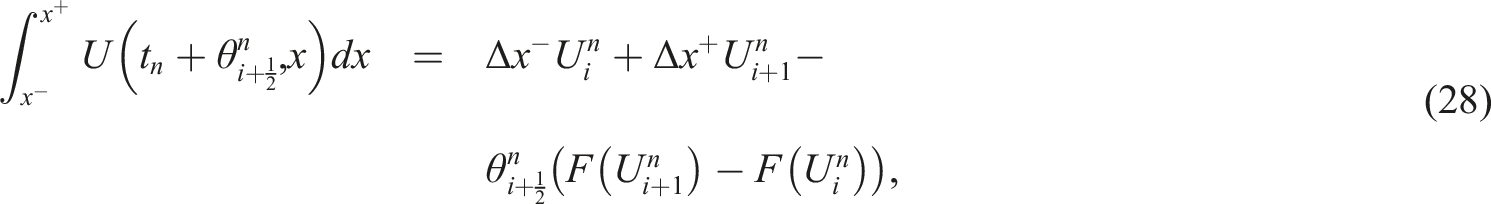
To get an approximation of $U_{i+\frac{1}{2}}^n$ , we adjust the mR technique given in^44–46 for conservation laws with source terms. To build $U_{i+\frac{1}{2}}^n$ that will be utilized in the corrector stage equation (25), we integrate equation (1) over a control domain $\left[t_n,t_n+{\theta }_{i+\frac{1}{2}}^n\right]\times \left[x^{-},x^{+}\right]$ . Here, $U_{i\pm \frac{1}{2}}^n$ is an approximation of Riemann solution R_s over the control volume [x⁻, x⁺] at $t_n+{\theta }_{i+\frac{1}{2}}^n$ . Hence, the resulting intermediate state is

$$\begin{array}{lll}{\displaystyle {\int }_{x^{-}}^{x^{+}}U\left(t_n+{\theta }_{i+\frac{1}{2}}^n,x\right)dx}\hfill & =\hfill & \mathrm{\Delta }{x}^{-}{U}_i^n+\mathrm{\Delta }{x}^{+}{U}_{i+1}^n-\hfill \\ \hfill & \hfill & {\theta }_{i+\frac{1}{2}}^n\left(F\left(U_{i+1}^n\right)-F\left(U_i^n\right)\right),\hfill \end{array}$$

(28)

where the distance measures are defined by

$$\mathrm{\Delta }{x}^{-}=\left|x^{-}-x_{i+\frac{1}{2}}\right|,\hspace{1em}\mathrm{\Delta }{x}^{+}=\left|x^{+}-x_{i+\frac{1}{2}}\right|.$$

We put x⁻ = x_i and x⁺ = x_i+1 in equation (28), then the predictor stage is given by

$$U_{i+\frac{1}{2}}^n=\frac{1}{2}\left(U_i^n+U_{i+1}^n\right)-\frac{{\theta }_{i+\frac{1}{2}}^n}{\mathrm{\Delta }x}\left(F\left(U_{i+1}^n\right)-F\left(U_i^n\right)\right),$$

(29)

where $U_{i+\frac{1}{2}}^n$ is an approximate average of solution U in control domain $\left[t_n,t_n+{\theta }_{i+\frac{1}{2}}^n\right]\times \left[x_i,x_{i+1}\right]$ defined as

$$U_{i+\frac{1}{2}}^n=\frac{1}{\mathrm{\Delta }x}{\displaystyle {\int }_{x_i}^{x_{i+1}}U}\left(x,t_n+{\theta }_{i+\frac{1}{2}}^n\right)dx.$$

(30)

To finish the structure of the mR scheme, the time parameter ${\theta }_{i+\frac{1}{2}}^n$ has to be chosen. The choosing of parameter ${\theta }_{i+\frac{1}{2}}^n$ relies on the stability analysis given in.[38] The variable ${\theta }_{j+1/2}^n$ is given by

$${\theta }_{i+\frac{1}{2}}^n={\alpha }_{i+\frac{1}{2}}^n\frac{\mathrm{\Delta }x}{2S_{i+\frac{1}{2}}^n}$$

(31)

where ${\alpha }_{i+\frac{1}{2}}^n$ is a local parameter to be determined locally, whereas $S_{i+\frac{1}{2}}^n$ is local Rusanov velocity defined as

$$S_{i+\frac{1}{2}}^n=\underset{k=1,\dots ,K}{\text{max}}\left(\text{max}\left(\mathrm{\mid }{\mathrm{\lambda }}_{k,i}^n\mathrm{\mid },\mathrm{\mid }{\mathrm{\lambda }}_{k,i+1}^n\mathrm{\mid }\right)\right),$$

(32)

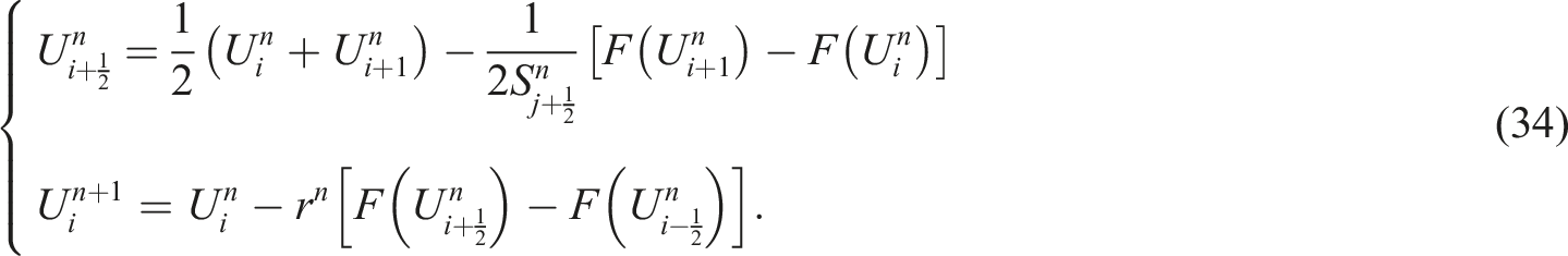
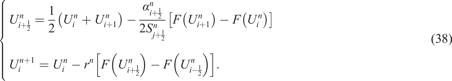
with ${\mathrm{\lambda }}_{k,i}^n$ is the k-th eigenvalue in equation (5). Thus, the predictor stage equation (29) can be represented as follows

$$U_{i+\frac{1}{2}}^n=\frac{1}{2}\left(U_i^n+U_{i+1}^n\right)-\frac{{\alpha }_{i+\frac{1}{2}}^n}{2S_{j+\frac{1}{2}}^n}\left[F\left(U_{i+1}^n\right)-F\left(U_i^n\right)\right].$$

(33)

It is clear that ${\alpha }_{i+\frac{1}{2}}^n=\frac{\mathrm{\Delta }t}{\mathrm{\Delta }x}{S}_{j+\frac{1}{2}}^n$ one recovers the Lax–Wendroff technique ⁴⁷ and ${\alpha }_{i+\frac{1}{2}}^n=1$ in the linear case the mR scheme goes to classical Rusanov scheme ⁴⁸ and in the nonlinear case one goes to first-order scheme written as the following

$$\{\begin{array}{l}{U}_{i+\frac{1}{2}}^n=\frac{1}{2}\left(U_i^n+U_{i+1}^n\right)-\frac{1}{2S_{j+\frac{1}{2}}^n}\left[F\left(U_{i+1}^n\right)-F\left(U_i^n\right)\right]\hfill \\ U_i^{n+1}=U_i^n-r^n\left[F\left(U_{i+\frac{1}{2}}^n\right)-F\left(U_{i-\frac{1}{2}}^n\right)\right].\hfill \end{array}$$

(34)

Another choice of the slopes ${\alpha }_{i+\frac{1}{2}}^n$ can be written as

$${\alpha }_{i+\frac{1}{2}}^n=\left(1-\mathrm{\Phi }\left(r_{i+\frac{1}{2}}\right)\right)\frac{S_{i+\frac{1}{2}}^n}{s_{i+\frac{1}{2}}^n}+\frac{\mathrm{\Delta }t}{\mathrm{\Delta }x}{S}_{i+\frac{1}{2}}^n\mathrm{\Phi }\left(r_{i+\frac{1}{2}}\right),$$

(35)

$s_{i+\frac{1}{2}}^n=\underset{k=1,\dots ,K}{\text{min}}\left(\text{max}\left(\mathrm{\mid }{\mathrm{\lambda }}_{k,i}^n\mathrm{\mid },\mathrm{\mid }{\mathrm{\lambda }}_{k,i+1}^n\mathrm{\mid }\right)\right)$ ; ${\mathrm{\Phi }}_{i+\frac{1}{2}}=\mathrm{\Phi }\left(r_{i+\frac{1}{2}}\right)$ is an appropriate limiter that defined by using a flux limiter function Φ acting on a quantity, which measures the ratio $r_{i+\frac{1}{2}}=\frac{U_{i+1-q}-U_{i-q}}{U_{i+1}-U_i},q=\text{sign}\left[F^{\prime }\left(U_{i+\frac{1}{2}}^n\right)\right]$ of the upwind varies to the local change by utilizing Riemann invariants in equations (21) and (22). ⁴⁹ Here, the van Albada function

$$\mathrm{\Phi }\left(r\right)=\frac{r+r^2}{1+r^2}$$

(36)

and Minmod function

$$\mathrm{\Phi }\left(r\right)=\text{max}\left(0,\text{min}\left(1,r\right)\right)$$

(37)

are utilized. The limiter functions for example Van Leer or Superbee functions can be utilized.^47,50 Finally, we formulate mR scheme of equation (1) as follows

$$\{\begin{array}{l}{U}_{i+\frac{1}{2}}^n=\frac{1}{2}\left(U_i^n+U_{i+1}^n\right)-\frac{{\alpha }_{i+\frac{1}{2}}^n}{2S_{j+\frac{1}{2}}^n}\left[F\left(U_{i+1}^n\right)-F\left(U_i^n\right)\right]\hfill \\ U_i^{n+1}=U_i^n-r^n\left[F\left(U_{i+\frac{1}{2}}^n\right)-F\left(U_{i-\frac{1}{2}}^n\right)\right].\hfill \end{array}$$

(38)

Numerical results

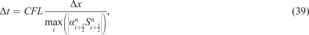
We introduce numerical simulation to isothermal Euler equations to validate the efficiency of the mR scheme by using Matlab Release 18. We take the following CFL condition with time step Δt

$$\mathrm{\Delta }t=CFL\frac{\mathrm{\Delta }x}{\underset{i}{\max }\left(\left|{\alpha }_{i+\frac{1}{2}}^n{S}_{i+\frac{1}{2}}^n\right|\right)},$$

(39)

CFL is a constant to be taken less than one.

Test 1

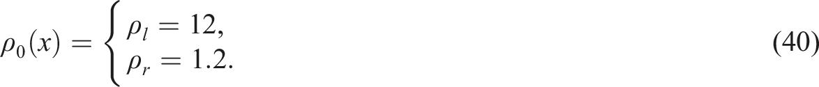
In the first test, we consider a Riemann problem with the following initial condition

$${\rho }_0\left(x\right)=\{\begin{array}{l}{\rho }_l=12,\hfill \\ {\rho }_r=\mathrm{1.2.}\hfill \end{array}$$

(40)

$$u_0\left(x\right)=\{\begin{array}{l}{u}_l=u_r=0.\hfill \end{array}$$

(41)

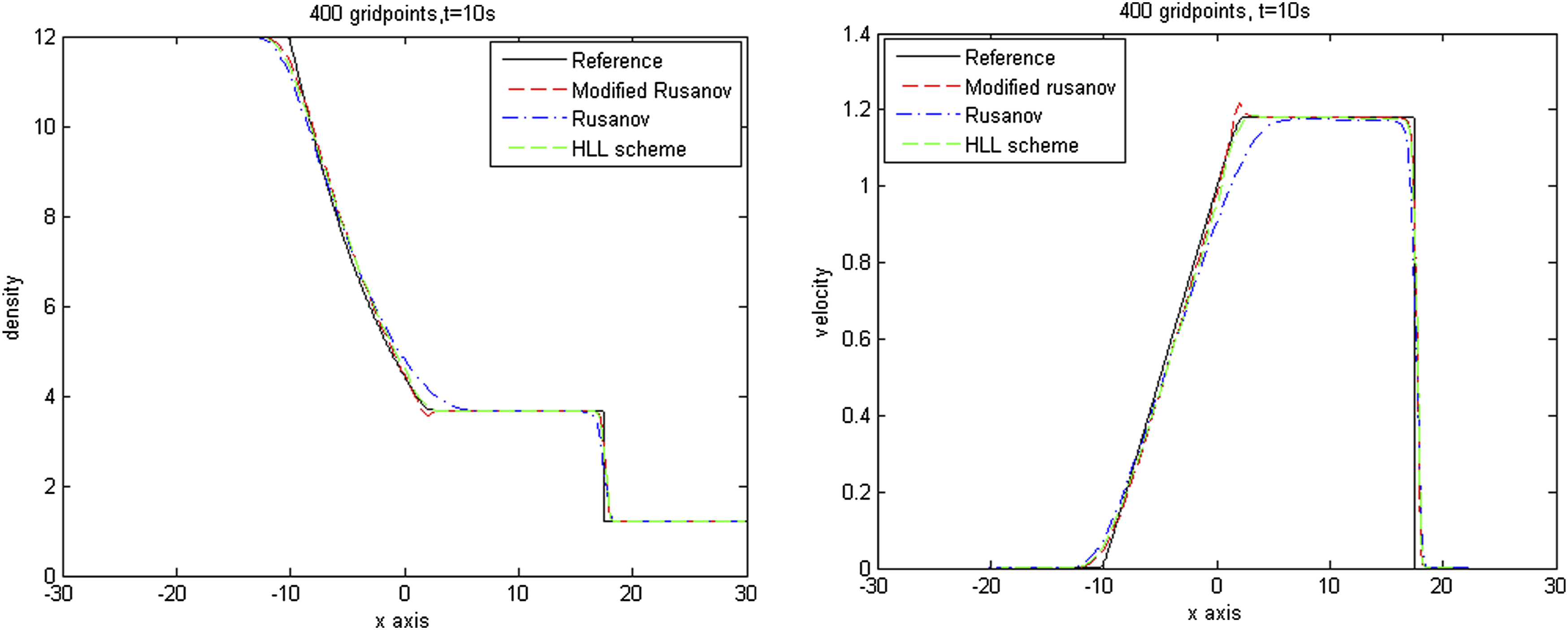
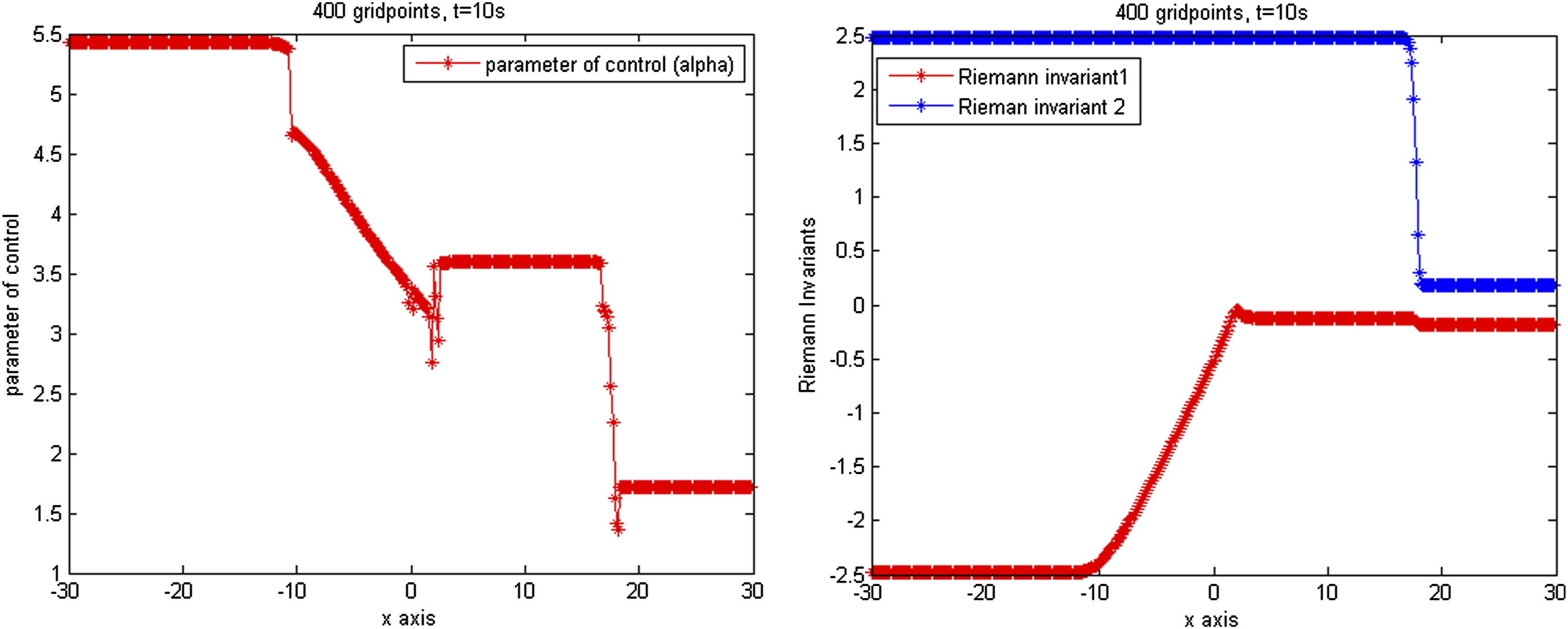
The solution consists of a rarefaction followed by a shock. We implement the mR scheme, classical Rusanov, and HLL schemes, utilizing 400 mesh points at time t = 10s. Figure 1 displays that the density and velocity for the mR scheme with limiter parameter of control, the Rusanov scheme, and HLL scheme with reference solution on 20000 gridpoints. We note that the results of Rusanov scheme are less accurate than mR and HLL schemes, whereas all the three schemes capable of capture the rarefaction and shock waves. The left part of Figure 2 shows the variation of parameter of control ${\alpha }_{i+\frac{1}{2}}^n$ , whereas right part illustrates the variation of Riemann invariants.

Figure 1.

Density (left) and velocity wave (right) at t = 10s.

Figure 2.

Parameter of control ${\alpha }_{i+\frac{1}{2}}^n$ (left) and Riemann invariants (right) at t = 10s.

Test 2

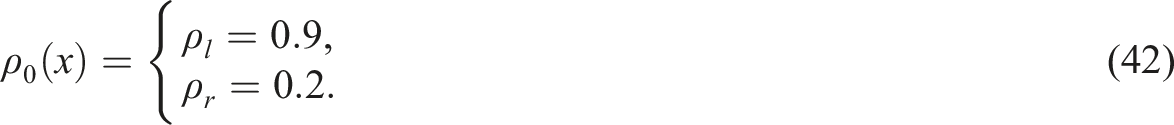
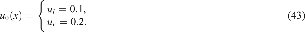
In the second test case, we present a Riemann problem with the following initial condition

$${\rho }_0\left(x\right)=\{\begin{array}{l}{\rho }_l=0.9,\hfill \\ {\rho }_r=\mathrm{0.2.}\hfill \end{array}$$

(42)

$$u_0\left(x\right)=\{\begin{array}{l}{u}_l=0.1,\hfill \\ u_r=\mathrm{0.2.}\hfill \end{array}$$

(43)

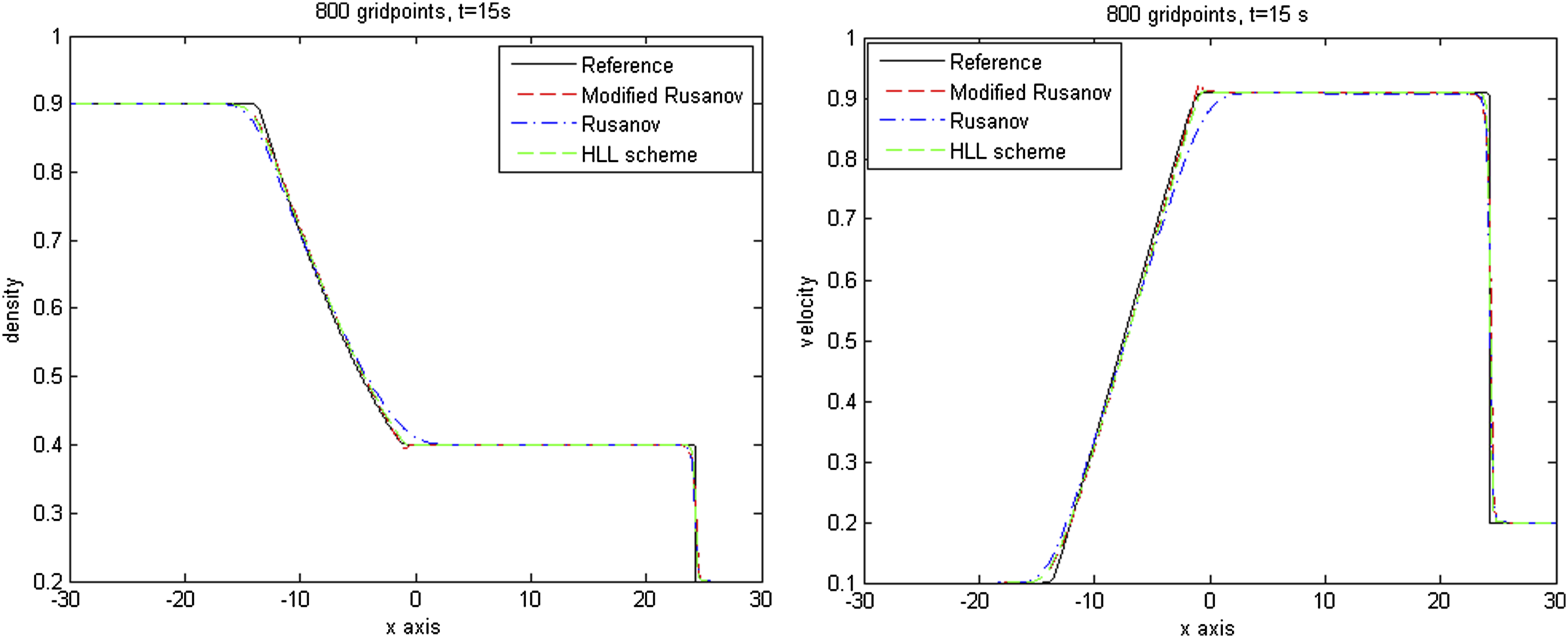
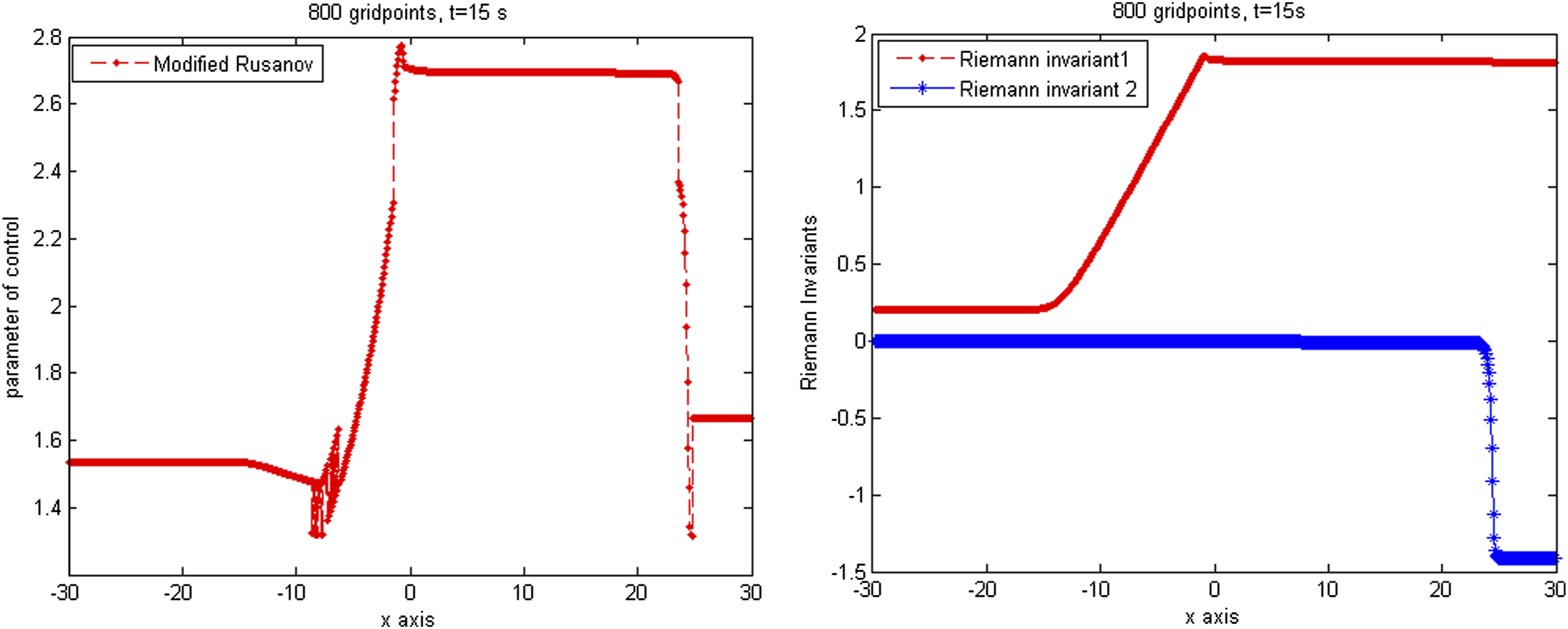
We implemented the mR scheme, classical Rusanov, and HLL scheme for isothermal equations, utilizing 800 mesh points at time t = 15s and the solution of this test case consists of a rarefaction followed by a shock. Figure 3 shows the density and velocity profile for three schemes and reference solution on 20000 gridpoints. We note that the mR method is more accurate than the Rusanov method and is as accurate as HLL scheme; also, the three schemes are capable of capturing the rarefaction and shock waves. The left part of from the Figure 4 shows the variation of parameter of control ${\alpha }_{i+\frac{1}{2}}^n$ , whereas right part shows the variation of Riemann invariants.

Figure 3.

Density (left) and velocity wave (right) at t = 15s.

Figure 4.

Parameter of control ${\alpha }_{i+\frac{1}{2}}^n$ (left) and Riemann invariants (right) at t = 15s.

Test 3

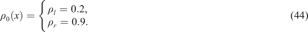
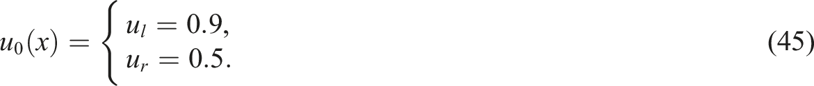
This test case was introduced in [51] and consists of a one-dimensional rectangle tube a shock; we present a Riemann problem with the following initial condition

$${\rho }_0\left(x\right)=\{\begin{array}{l}{\rho }_l=0.2,\hfill \\ {\rho }_r=\mathrm{0.9.}\hfill \end{array}$$

(44)

$$u_0\left(x\right)=\{\begin{array}{l}{u}_l=0.9,\hfill \\ u_r=\mathrm{0.5.}\hfill \end{array}$$

(45)

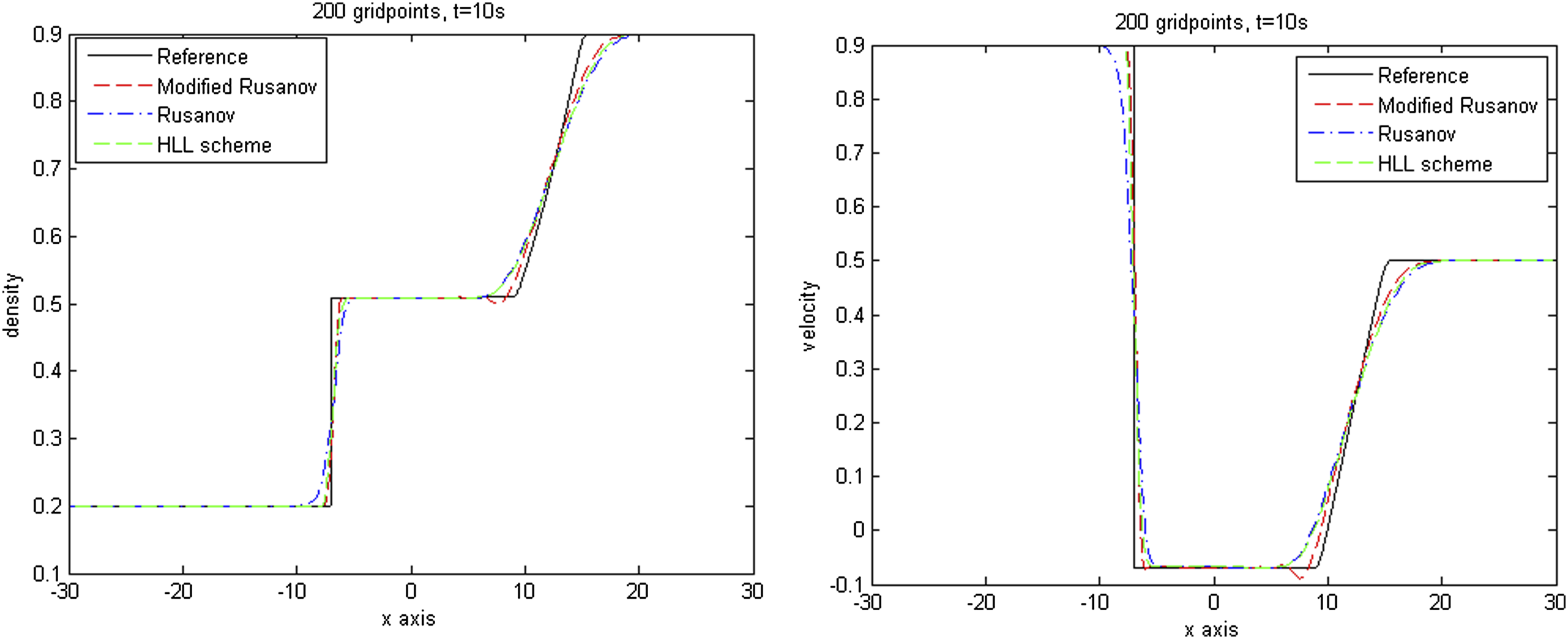
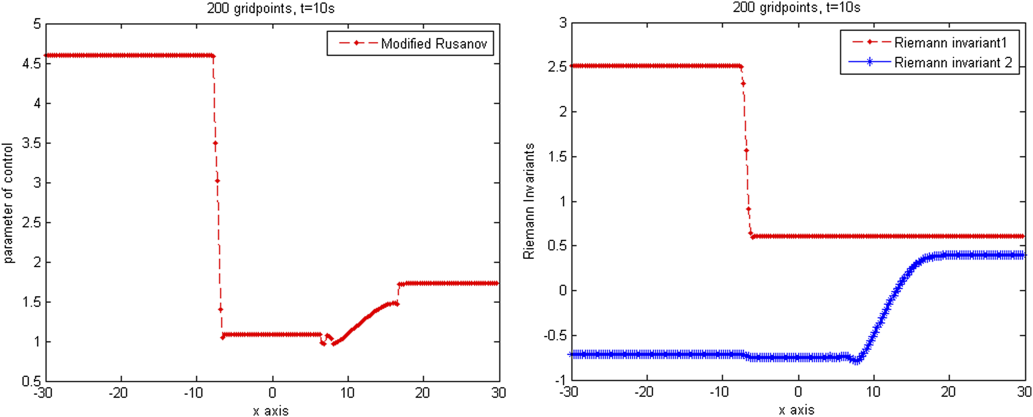
The solution of this test case consists of a shock followed by a rarefaction, utilizing 200 mesh points at time t = 10s. Figure 5 shows the comparison of density and velocity profile, using three schemes and reference solution on 20000 gridpoints. The left part of from the Figure 6 shows the variation of parameter of control ${\alpha }_{i+\frac{1}{2}}^n$ , whereas right part depicts the variation of Riemann invariants.

Figure 5.

Density (left) and velocity wave (right) at t = 10s.

Figure 6.

Parameter of control ${\alpha }_{i+\frac{1}{2}}^n$ (left) and Riemann invariants (right) at t = 10s.

Conclusions

We have investigated the isothermal Euler model with non-vacuum initial data. The derivation of Riemann invariants corresponding for the isothermal Euler model is introduced. The mR scheme was introduced for solving the 1-D initial value problems for the isothermal Euler model. This scheme has substantially different technical structure from the well-known schemes like finite difference. For comparison, Rusanov scheme was also implemented for solving the proposed model. Our results show that the results of the mR scheme are better and more accurate. Hence, it is concluded that mR scheme is a robust and efficient technique for solving such models.

Despite this success, this work is still a preliminary development of the isothermal Euler model. A more feasible way is to develop new conserved scheme for the 2D isothermal Euler system. We also consider the interaction of the elementary waves for the isothermal Euler model, which will be done in the future work.