Numerical investigation to the full URE equations via predictor-corrector scheme

Abstract

We produce the modified Rusanov (mR) method for the full ultra-relativistic Euler (URE) model. This system describes the flow of an ideal fluid of pressure $\mathsf{p}$ , spatial part $\mathsf{u}\in {\mathbb{R}}^3$ of the dimensionless four-velocity and particle density $\mathsf{n}$ . The nonlinear system in question is purely hyperbolic. The mR method is formulated as predictor and corrector phases. The predictor is based on the parameter of control $({\alpha }_{i+1/2}^n)$ , which is accountable for this scheme’s numerical diffusion. The balance conservation equation is reinstated by the corrector phase. Without utilizing Riemann problem solvers, the approach has the ability to compute the numerical flow that’s closest to the solution’s actually state. In the numerical simulation the results acquired via the mR method are compared with the Rusanov, the Lax-Friedrichs methods and reference solution with 10000 grid points calculated employing classical Rusanov. This numerical study confirms the effectiveness of the mR scheme. The mR technique can also be implemented to solve numerous other applied science models.

Introduction

These days, particle beams, astrophysics, high-energy nuclear physics, and free-electron technology for lasers all depend on relativistic gas dynamics. The relativistic Euler system is a generalization of the Euler model that account for the influences of special relativity in fluid mechanics and astronomy. This system depicts relativistic gas dynamics is inherently nonlinear, making analytical approaches to actual issues difficult to find. Instead, numerical solutions are typically attempted.^1–4 Furthermore, the existence of relativistic motion causes resistive effects to differ qualitatively and quantitatively from those observed in the Newtonian regime. There are certain numerical methods for solving relativistic equations that provide severe discontinuities for shock fronts and high order accuracy in fluid flow simulations’ smooth zones.^5–10

Nonlinear waves have lately acquired significance in nonlinear research due to their ability to minaret several complex phenomena with important applications.^11–15 Since nonlinear systems are extremely challenging to solve analytically, numerical techniques are widely used to calculate their approximate solutions.^16–19 In applied research, numerous kinds of nonlinear partial differential equations regulate a variety of flow fields including complicated phenomena.^20–23 Complex interactions between nonlinear waves can be observed in realistic systems with conservation laws. This intricacy is a significant barrier to comprehension of Riemann initial-data problem solutions. The mathematical framework of hyperbolic conservation principles appears in many diverse fields, including biology, elasticity, energy, oceanography, flow in porous media, and numerous other areas. Many flow fields that contain wave events are controlled by hyperbolic nonlinear systems that are quasi-linear.^24–27 Additionally, these models offer a wealth of fascinating partial differential equation-based mathematics problems.

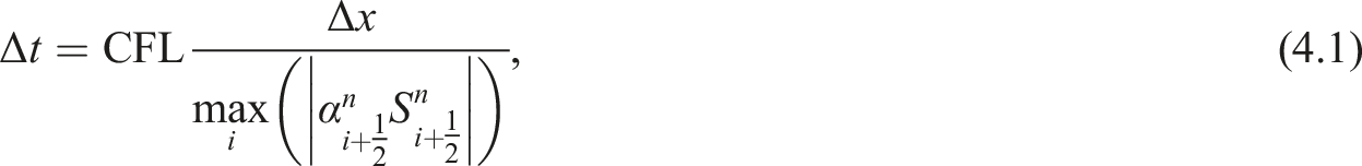
The modified Rusanov (mR) strategy is used in this article to solve the URE system. There are predictor and corrector steps in this method. Riemann invariants and limiters theory are used to govern a numerical diffusion control parameter in the predictor stage. The equation for balance conservation is retrieved in the second step. The study of stability showed that, depending on the choice of the control parameter, the mR method might be of order 1 or 2. ²⁸ The numerical results of the original Rusanov and the Lax-Friedrichs methods are also implemented for validation and comparison. The time step size is determined by the Courant-Friedrich-Lewy stability criteria, wherein no gas beam may physically pass across more than one cell gap in a single time step. Numerous numerical test cases are executed, which show that the mR technique is extremely effective and potent.

The following is the article’s structure. Section 2 presents the URE model. In Section 3, the mR method for solving the URE system is abbreviated. Section 4 introduces the numerical results through nine test cases. Section 5 contains further demonstration for the generated numerical outcomes. We offer observations and conclusions regarding the current findings in Section 6.

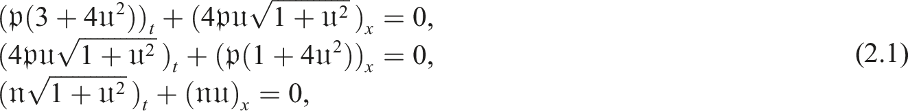
The mathematical model for URE

The mathematical model for URE in conservation form for energy, momentum, and mass is given as follows^29,30:

$\begin{array}{c}{(\mathfrak{p}(3+4{\mathfrak{u}}^2))}_t+{(4\mathfrak{p}\mathfrak{u}\sqrt{1+{\mathfrak{u}}^2})}_x=0,\hfill \\ {(4\mathfrak{p}\mathfrak{u}\sqrt{1+{\mathfrak{u}}^2})}_t+{(\mathfrak{p}(1+4{\mathfrak{u}}^2))}_x=0,\hfill \\ {(\mathfrak{n}\sqrt{1+{\mathfrak{u}}^2})}_t+{(\mathfrak{n}\mathfrak{u})}_x=0,\hfill \end{array}$

(2.1)

$\mathfrak{p}>0$ ; $\mathtt{v}=\mathfrak{u}/\sqrt{1+{\mathfrak{u}}^2}$ symbolize pressure and velocity, $\mid \mathtt{v}\mid <1$ , $\mathfrak{u}\in \mathbb{R}$ .

The eigenvalues of model (2.1) are

${\gamma }_1=\frac{2\mathfrak{u}\sqrt{1+{\mathfrak{u}}^2}-\sqrt{3}}{3+2{\mathfrak{u}}^2}<{\gamma }_2=\frac{\mathfrak{u}}{\sqrt{1+{\mathfrak{u}}^2}}<{\gamma }_3=\frac{2\mathfrak{u}\sqrt{1+{\mathfrak{u}}^2}+\sqrt{3}}{3+2{\mathfrak{u}}^2}.$

(2.2)

Proposition 2.1

²⁹ For $\mathfrak{p}>0$ ; $\mathfrak{u}\in \mathbb{R}$ and $\mathfrak{n}>0$ , the URE system (2.1) exhibits strict hyperbolicity. Additionally, the second defining field exhibits linear degeneration, and genuinely nonlinearity is present in the first and third characteristic fields.

The conditions for the Rankine-Hugoniot jump are

$\begin{array}{c}s\left[{\mathfrak{p}}_{+}(3+4{\mathfrak{u}}_{+}^2)-{\mathfrak{p}}_{-}(3+4{\mathfrak{u}}_{-}^2)\right]=4{\mathfrak{p}}_{+}{\mathfrak{u}}_{+}\sqrt{1+{\mathfrak{u}}_{+}^2}-4{\mathfrak{p}}_{-}{\mathfrak{u}}_{-}\sqrt{1+{\mathfrak{u}}_{-}^2},\hfill \\ s\left[4{\mathfrak{p}}_{+}{\mathfrak{u}}_{+}\sqrt{1+{\mathfrak{u}}_{+}^2}-4{\mathfrak{p}}_{-}{\mathfrak{u}}_{-}\sqrt{1+{\mathfrak{u}}_{-}^2}\right]={\mathfrak{p}}_{+}(1+4{\mathfrak{u}}_{+}^2)-{\mathfrak{p}}_{-}(1+4{\mathfrak{u}}_{-}^2),\hfill \\ s\left[{\mathfrak{n}}_{+}\sqrt{1+{\mathfrak{u}}_{+}^2}-{\mathfrak{n}}_{-}\sqrt{1+{\mathfrak{u}}_{-}^2}\right]={\mathfrak{n}}_{+}{\mathfrak{u}}_{+}-{\mathfrak{n}}_{-}{\mathfrak{u}}_{-},\hfill \end{array}$

(2.3)

with a constant velocity s, in which $({\mathfrak{p}}_{-},{\mathfrak{u}}_{-},{\mathfrak{n}}_{-})$ ; $({\mathfrak{p}}_{+},{\mathfrak{u}}_{+},{\mathfrak{n}}_{+})$ are the shock’s constant left and right states when ${\mathfrak{p}}_{\pm }>0$ . The entropy inequality is

$-s({\mathrm{\Psi }}_{+}-{\mathrm{\Psi }}_{-})+({\mathrm{\Phi }}_{+}-{\mathrm{\Phi }}_{-})>0,$

(2.4)

that is equivalent to ${\mathfrak{u}}_{-}>{\mathfrak{u}}_{+}$ , ³¹ where

$\begin{array}{c}\mathrm{\Psi }(\mathfrak{p},\mathfrak{u},\mathfrak{n})=-\mathfrak{n}\sqrt{1+{\mathfrak{u}}^2}\ln \frac{{\mathfrak{n}}^4}{{\mathfrak{p}}^3},\mathrm{\Phi }(\mathfrak{p},\mathfrak{u},\mathfrak{n})=-\mathfrak{n}\mathfrak{u}\ln \frac{{\mathfrak{n}}^4}{{\mathsf{p}}^3}.\hfill \end{array}$

(2.5)

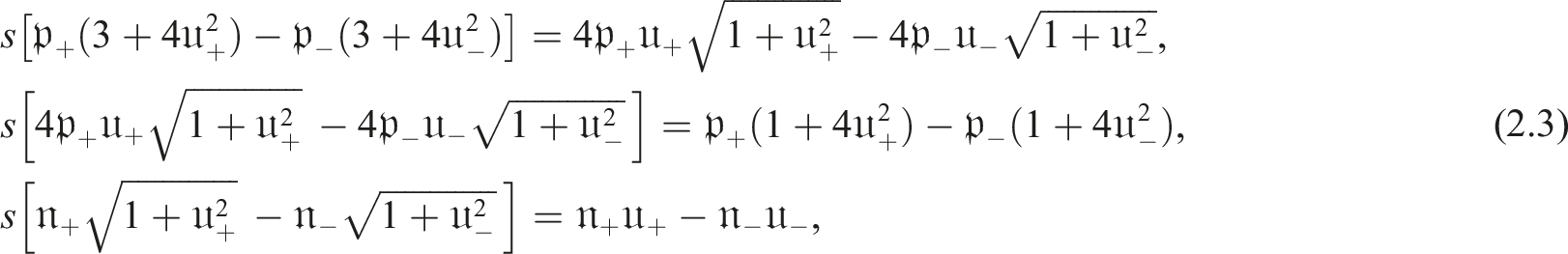
We consult ¹⁰ for more information on the parameters of elementary waves.

Brief description of the mR scheme

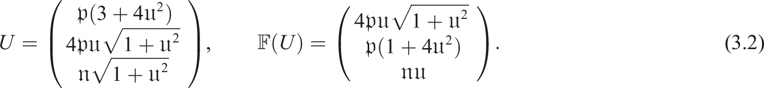
New, we rewrite the Eqs. (2.1) in following conservation form

$\frac{\partial U}{\partial t}+\frac{\partial \mathbb{F}(U)}{\partial x}=0,$

(3.1)

where $\mathbb{F}(U)$ and U denote the vector-value functions in R³, which can be written as the following

$U=\left(\begin{array}{c}\hfill \mathfrak{p}(3+4{\mathfrak{u}}^2)\hfill \\ \hfill 4\mathfrak{p}\mathfrak{u}\sqrt{1+{\mathfrak{u}}^2}\hfill \\ \hfill \mathfrak{n}\sqrt{1+{\mathfrak{u}}^2}\hfill \end{array}\right),\mathbb{F}(U)=\left(\begin{array}{c}\hfill 4\mathfrak{p}\mathfrak{u}\sqrt{1+{\mathfrak{u}}^2}\hfill \\ \hfill \mathfrak{p}(1+4{\mathfrak{u}}^2)\hfill \\ \hfill \mathfrak{n}\mathfrak{u}\hfill \end{array}\right).$

(3.2)

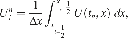
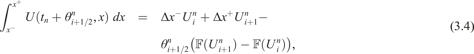
To present the modified Rusanov scheme, we integrate the equation (3.1) within the domain [t _n , t_n+1] × [x_i−1/2, x_i+1/2], we have the following finite volume method

$U_i^{n+1}=U_i^n-\frac{\mathrm{\Delta }t}{\mathrm{\Delta }x}\left(\mathbb{F}\left(U_{i+\frac{1}{2}}^n\right)-\mathbb{F}\left(U_{i-\frac{1}{2}}^n\right)\right),$

(3.3)

$U_i^n$ represents an average of the solutionsU in the range [x_i−1/2, x_i+1/2] at time t _n , that is,

$U_i^n=\frac{1}{\mathrm{\Delta }x}{\int }_{x_{i-\frac{1}{2}}}^{x_{i+\frac{1}{2}}}U(t_n,x)dx,$

and $\mathbb{F}(U_{i\pm 1/2}^n)$ represents the numerical flux at x = x_i±1/2 and time t _n . The fundamental of the finite volumes method is construction of the numerical fluxes, to build the numerical flux in the predictor phase.^28,32–35 Reintegrating equation (3.1) over the volume of control $[t_n,t_n+{\theta }_{i+1/2}^n]\times [x^{-},x^{+}]$ , ²⁶ produces

$\begin{array}{ccc}\hfill {\int }_{x^{-}}^{x^{+}}U(t_n+{\theta }_{i+1/2}^n,x)dx& =\hfill & \mathrm{\Delta }{x}^{-}{U}_i^n+\mathrm{\Delta }{x}^{+}{U}_{i+1}^n-\hfill \\ \hfill & \hfill & {\theta }_{i+1/2}^n\left(\mathbb{F}(U_{i+1}^n)-\mathbb{F}(U_i^n)\right),\hfill \end{array}$

(3.4)

where the solution U in the domain $[t_n,t_n+{\theta }_{i+1/2}^n]\times [x^{-},x^{+}]$ is approximated by $U_{i+1/2}^n=1/\mathrm{\Delta }{x}^{-}+\mathrm{\Delta }{x}^{+}{\int }_{x^{-}}^{x^{+}}U(x,t_n+{\theta }_{i+1/2}^n)dx$ , where Δx⁻ and Δx⁺ are distance measurements as

$\mathrm{\Delta }{x}^{-}=\left|x^{-}-x_{i+1/2}\right|,\mathrm{\Delta }{x}^{+}=\left|x^{+}-x_{i+1/2}\right|,$

which lead to write the predictor stage as the follows

$U_{i+\frac{1}{2}}^n=\frac{1}{2}\left(U_i^n+U_{i+1}^n\right)-\frac{{\alpha }_{i+\frac{1}{2}}^n}{2S_{i+\frac{1}{2}}^n}\left(\mathbb{F}(U_{i+1}^n)-\mathbb{F}(U_i^n)\right).$

(3.5)

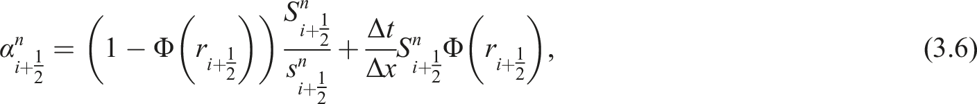
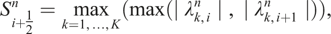
Actually, there are three choice for the parameter of control according to the analysis, namely in the linear case there are two choice and one choice in the nonlinear case, see 28. These choices given as follow:

(1) The first one is ${\alpha }_{i+1/2}^n=\mathrm{\Delta }t/\mathrm{\Delta }x{S}_{j+1/2}^n$ , then the scheme recovers the Lax-Wendroff scheme.

(2) The second one is ${\alpha }_{i+1/2}^n=1$ , then the scheme becomes the classical Rusanov scheme.

(3) The third one in the nonlinear case, the proposed scheme recovers the following first order scheme:

${\alpha }_{i+\frac{1}{2}}^n=\left(1-\mathrm{\Phi }\left(r_{i+\frac{1}{2}}\right)\right)\frac{S_{i+\frac{1}{2}}^n}{s_{i+\frac{1}{2}}^n}+\frac{\mathrm{\Delta }t}{\mathrm{\Delta }x}{S}_{i+\frac{1}{2}}^n\mathrm{\Phi }\left(r_{i+\frac{1}{2}}\right),$

(3.6)

where

$S_{i+\frac{1}{2}}^n=\underset{k=1,\dots ,K}{\text{max}}(\text{max}(\mid {\lambda }_{k,i}^n\mid ,\mid {\lambda }_{k,i+1}^n\mid )),$

$s_{i+1/2}^n=\underset{k=1,\dots ,K}{\text{min}}(\text{max}(\mid {\lambda }_{k,i}^n\mid ,\mid {\lambda }_{k,i+1}^n\mid ))$ and ${\mathrm{\Phi }}_{i+1/2}=\mathrm{\Phi }\left(r_{i+1/2}\right)$ is a suitable limiter, which is determined by applying the flux limiter functionΦ to a quantity, which calculates the ratio $r_{i+\frac{1}{2}}=\frac{W_{i+1-q}-W_{i-q}}{W_{i+1}-W_i},q=\mathrm{s}\mathrm{i}\mathrm{g}\mathrm{n}\left[F^{\prime }(W_{i+\frac{1}{2}}^n)\right]$ with ${\lambda }_{k,i}^n$ is the kth eigenvalues in Eqs. (2.1).

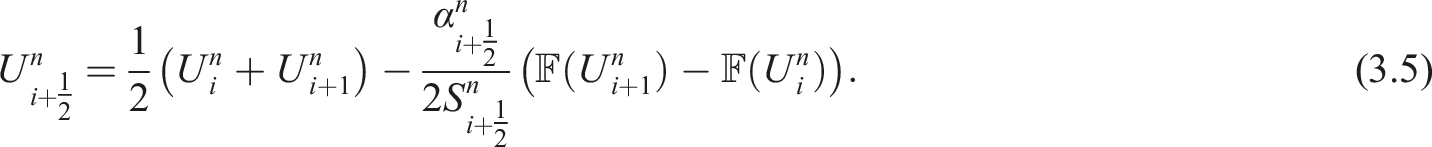
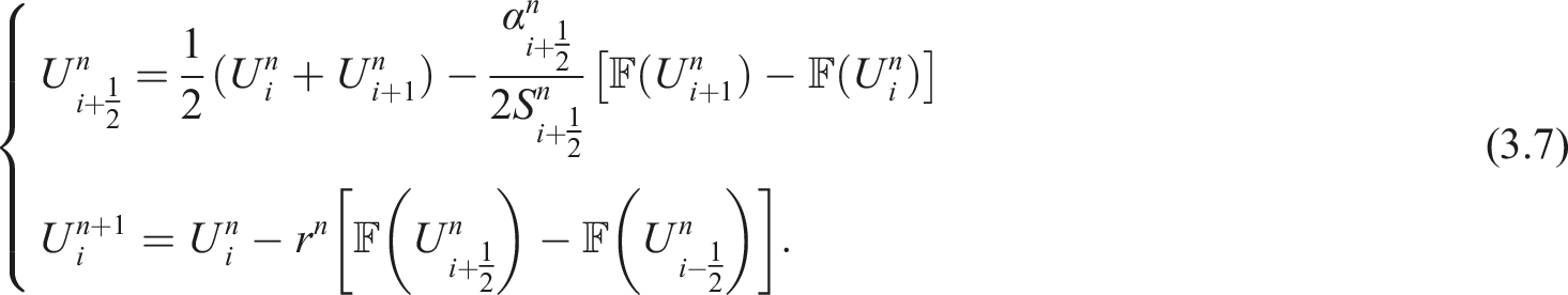
Finally, we can write the predictor and corrector modified Rusanov scheme for equation (3.1) as follows

$\left\{\begin{array}{c}{U}_{i+\frac{1}{2}}^n=\frac{1}{2}(U_i^n+U_{i+1}^n)-\frac{{\alpha }_{i+\frac{1}{2}}^n}{2S_{i+\frac{1}{2}}^n}\left[\mathbb{F}(U_{i+1}^n)-\mathbb{F}(U_i^n)\right]\hfill \\ U_i^{n+1}=U_i^n-r^n\left[\mathbb{F}\left(U_{i+\frac{1}{2}}^n\right)-\mathbb{F}\left(U_{i-\frac{1}{2}}^n\right)\right].\hfill \end{array}\right.$

(3.7)

The numerical simulation of the URE system

We present ninth numerical test cases, utilizing the mR scheme, classical Rusanov, Lax-Friedrichs scheme as well as a reference solution calculated using classical Rusanov with 10000 gridpoints for numerical simulation of the URE equations over the domain L = [0, 1]. In order to perform this numerical study, we choose the stability scenario ²⁸ in the next sense

$\mathrm{\Delta }t=\mathrm{CFL}\frac{\mathrm{\Delta }\mathsf{x}}{\underset{i}{\max }\left(\left|{\alpha }_{i+\frac{1}{2}}^n{S}_{i+\frac{1}{2}}^n\right|\right)},$

(4.1)

$\mathrm{CFL}=0.6$ .

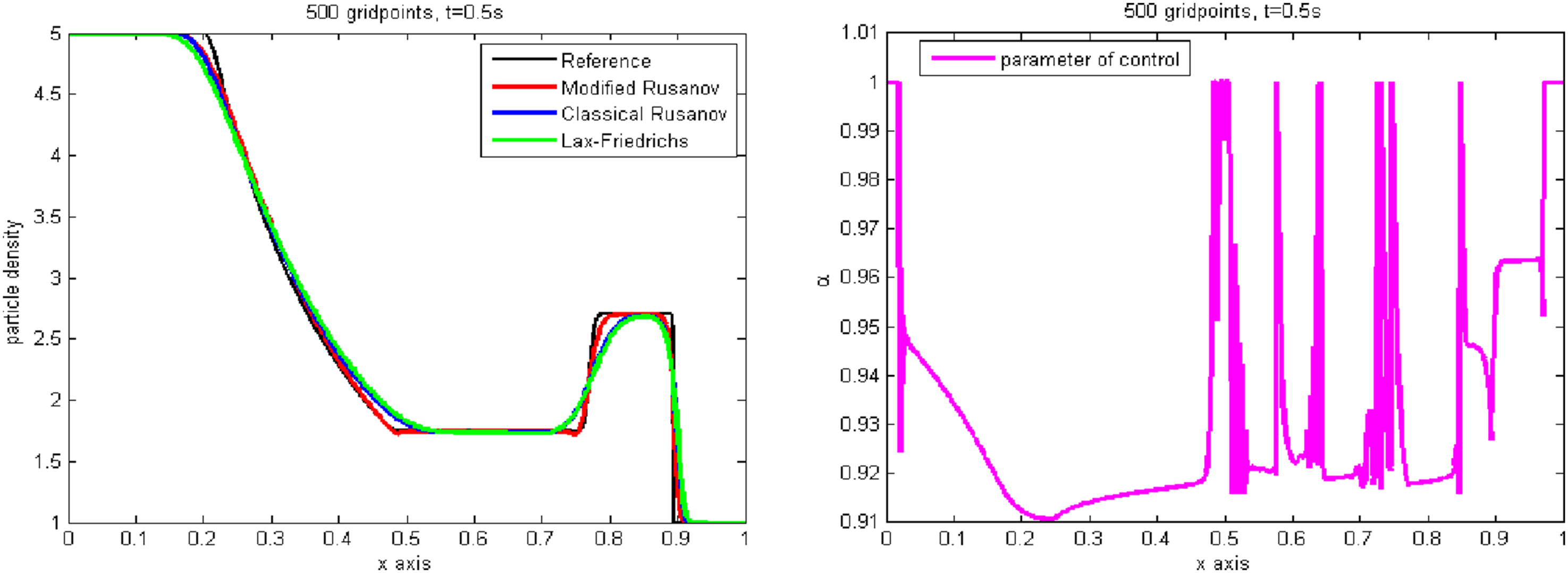
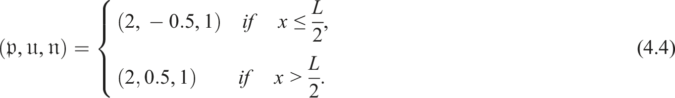
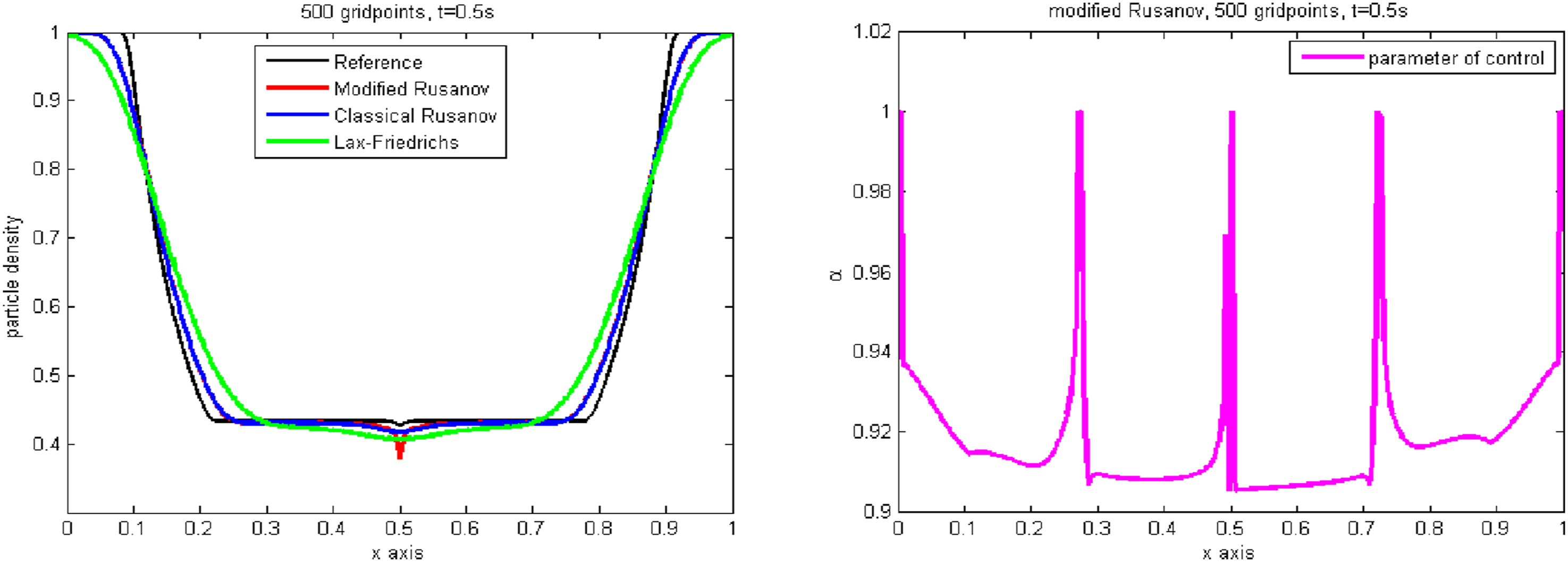
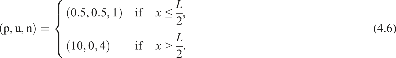
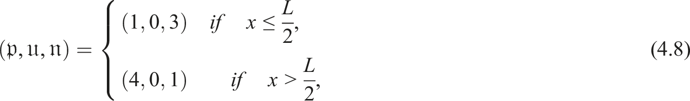
First test

We use the following initial conditions in this test case:

$(\mathfrak{p},\mathfrak{u},\mathfrak{n})=\left\{\begin{array}{c}(\mathrm{8,0,5})ifx\le \frac{L}{2},\hfill \\ (0.5,\mathrm{0,1})ifx>\frac{L}{2}.\hfill \end{array}\right.$

(4.2)

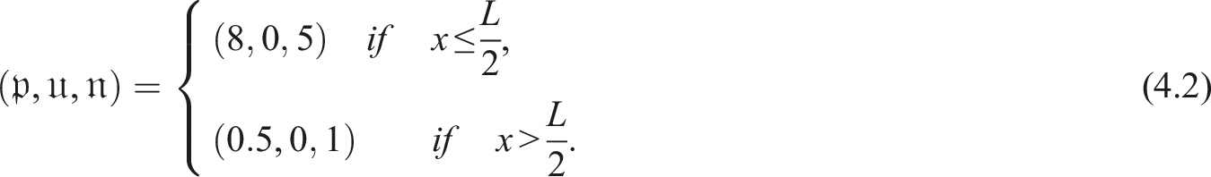
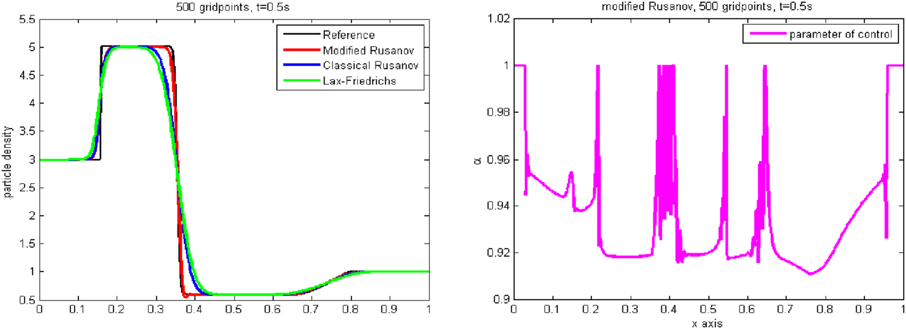
The solution to this problem involves an intermediate state bounded to the right by a shock wave and to the left by a transonic rarefaction wave. Figures 1 and 2 depict the propagation of the pressure, velocity, particle density, the control parameter’s variation ${\alpha }_{i+1/2}^n$ , respectively.

Figure 1.

Pressure, velocity at time t = 0.5 s.

Figure 2.

Particle density, 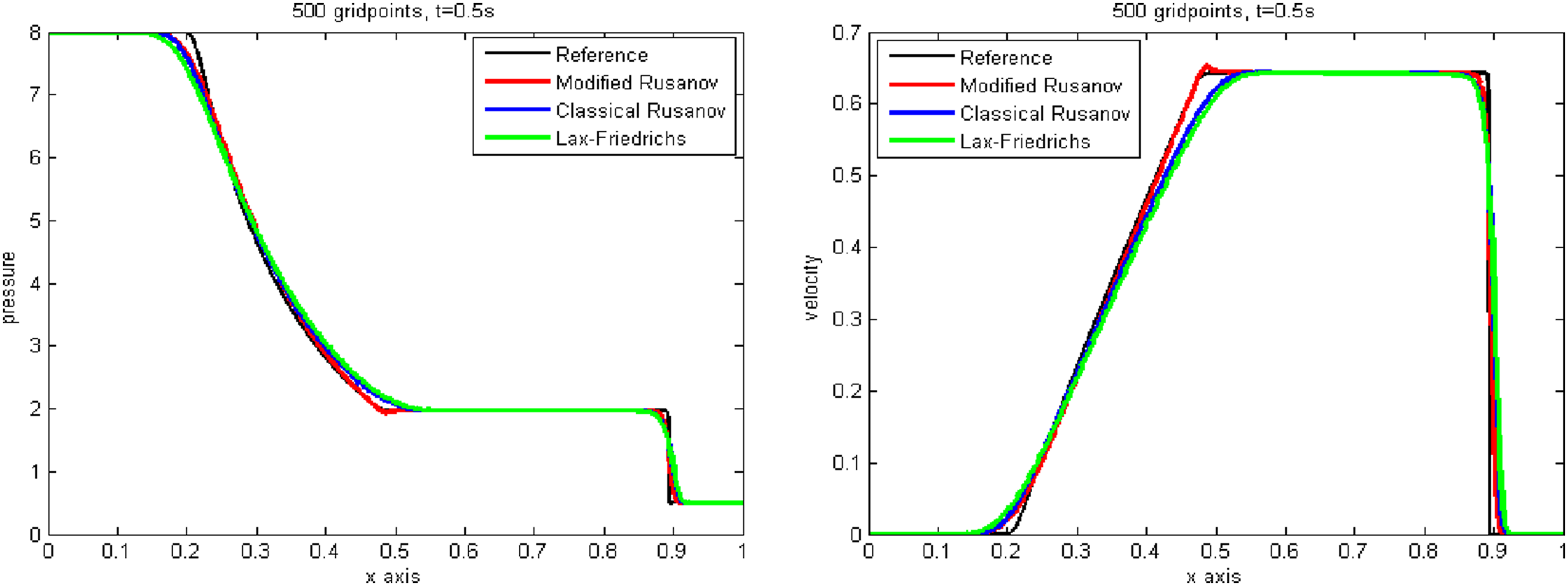${\alpha }_{i+1/2}^n$ is the control parameter at time t = 0.5 s.

Second test

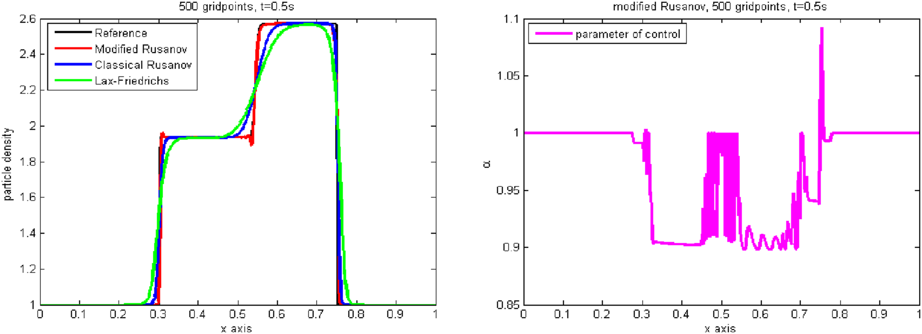
The initial data for this test case are as follows:

$(\mathfrak{p},\mathfrak{u},\mathfrak{n})=\left\{\begin{array}{c}(\mathrm{3,0.5},1)ifx\le \frac{L}{2},\hfill \\ (2,-0.5,1)ifx>\frac{L}{2}.\hfill \end{array}\right.$

(4.3)

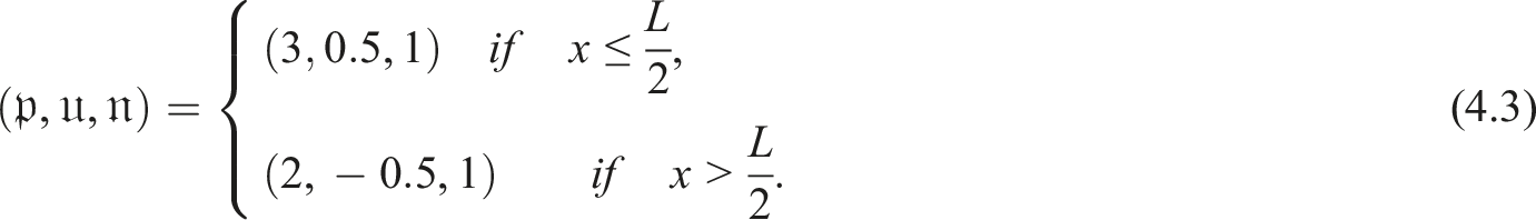
The solution is composed of two shock one traveling to let and the another traveling to left and the middle of two shock there is a contact discontinuity. Figures 3 and 4 illustrate the pressure, velocity, particle density, and variation of parameter of control, respectively.

Figure 3.

Pressure, speed wave at time t = 0.5 s.

Figure 4.

Particle density, controlling parameter 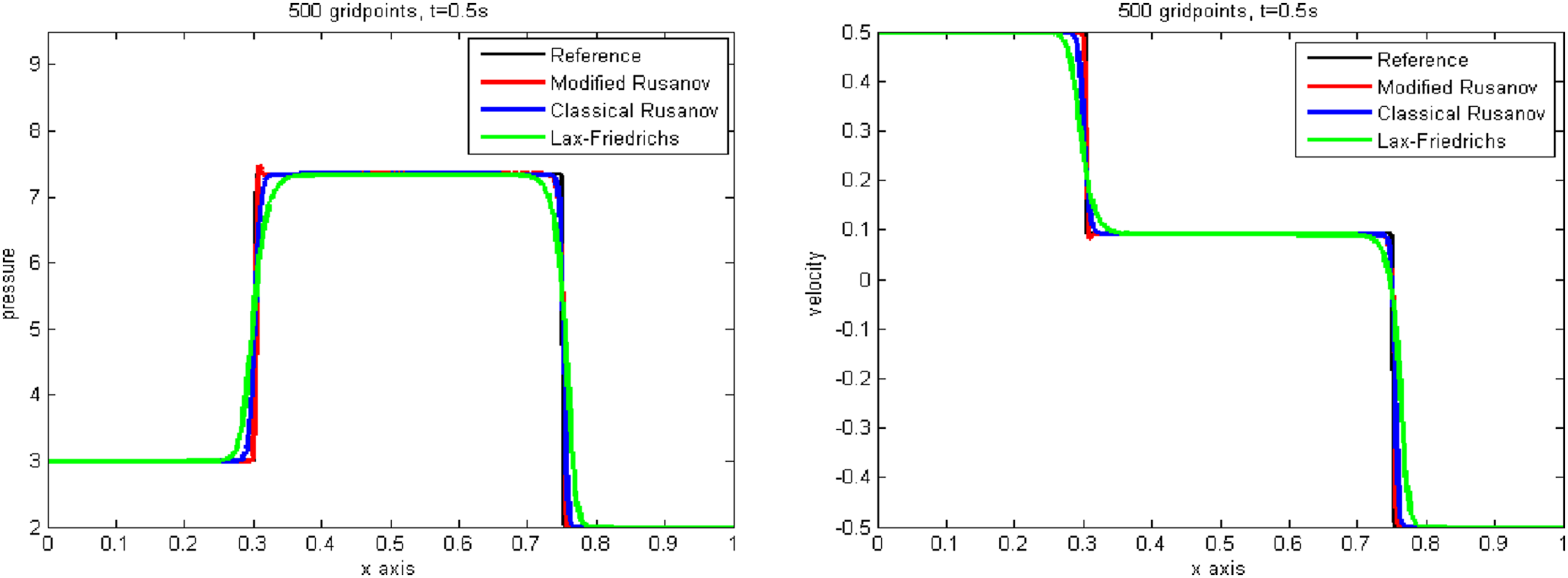${\alpha }_{i+1/2}^n$ at time t = 0.5 s.

Third test

We utilize the following as the initial conditions in this test case:

$(\mathfrak{p},\mathfrak{u},\mathfrak{n})=\left\{\begin{array}{c}(2,-0.5,1)ifx\le \frac{L}{2},\hfill \\ (\mathrm{2,0.5},1)ifx>\frac{L}{2}.\hfill \end{array}\right.$

(4.4)

This test case’s solution is composed of two strong rarefaction waves and a simple stationary contact discontinuity. Figures 5 and 6 illustrate the pressure, velocity, particle density, and variations in control parameters, respectively.

Figure 5.

Pressure, velocity at time t = 0.5 s.

Figure 6.

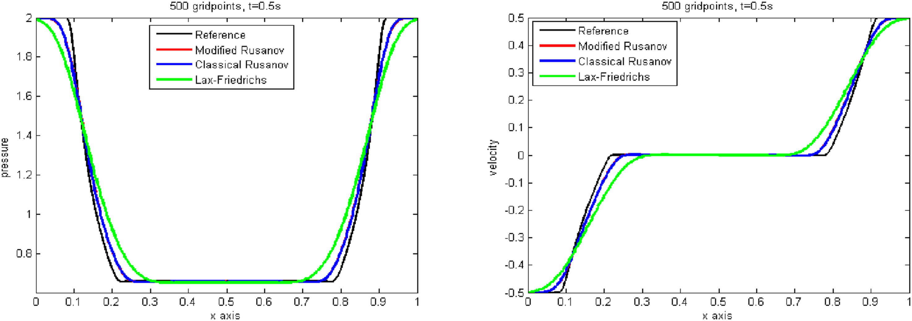
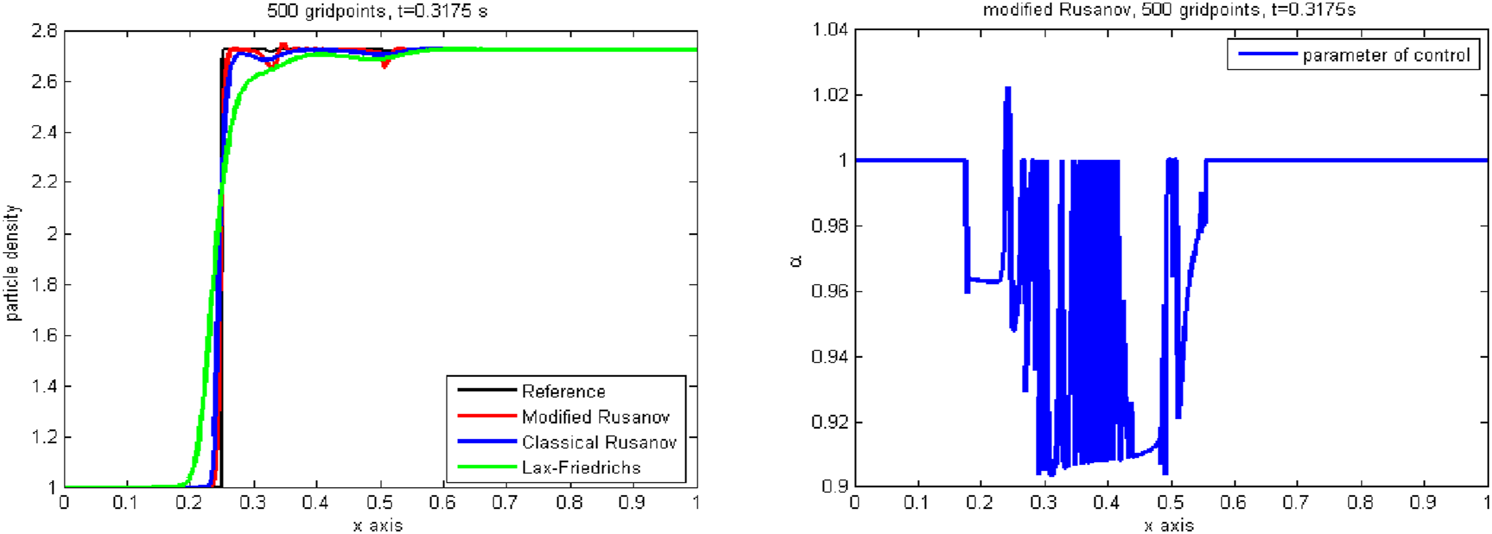
Particle density, ${\alpha }_{i+1/2}^n$ is the control parameter at time t = 0.5 s.

Fourth test

The initial data used in this test case are:

$(\mathfrak{p},\mathfrak{u},\mathfrak{n})=\left\{\begin{array}{c}(\mathrm{1,0.0},1)\text{if}x\le \frac{L}{2},\hfill \\ (4,-0.6495,2.725)\text{if}x>\frac{L}{2}.\hfill \end{array}\right.$

(4.5)

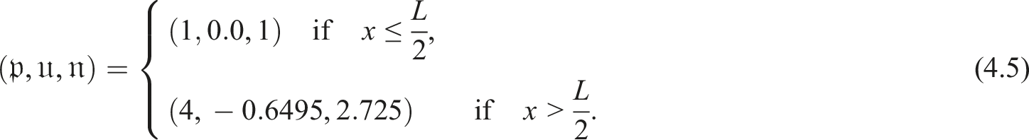
The solution comprises a single chock running from right to left. Figures 7 and 8 illustrate the pressure, velocity, particle density, and control parameter variation, respectively.

Figure 7.

Pressure, velocity at t = 0.3175 s.

Figure 8.

Particle density, controlling parameter 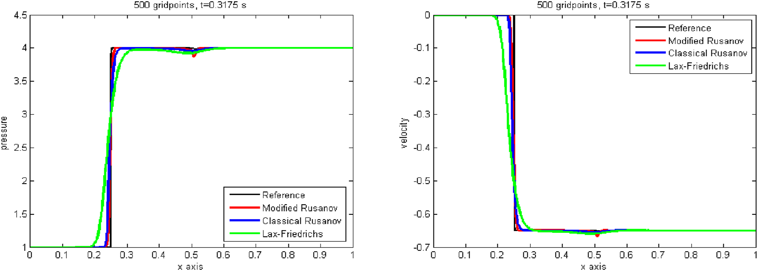${\alpha }_{i+1/2}^n$ at time t = 0.3175 s.

Fifth test

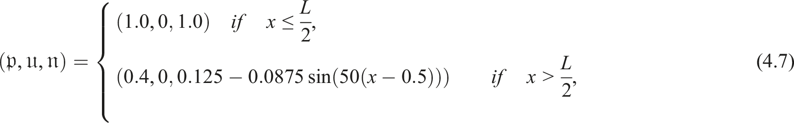
The initial conditions in this test case are as follows:

$(\mathrm{p},\mathrm{u},\mathrm{n})=\left\{\begin{array}{c}(0.5,0.5,1)\text{if}x\le \frac{L}{2},\hfill \\ (\mathrm{10,0,4})\text{if}x>\frac{L}{2}.\hfill \end{array}\right.$

(4.6)

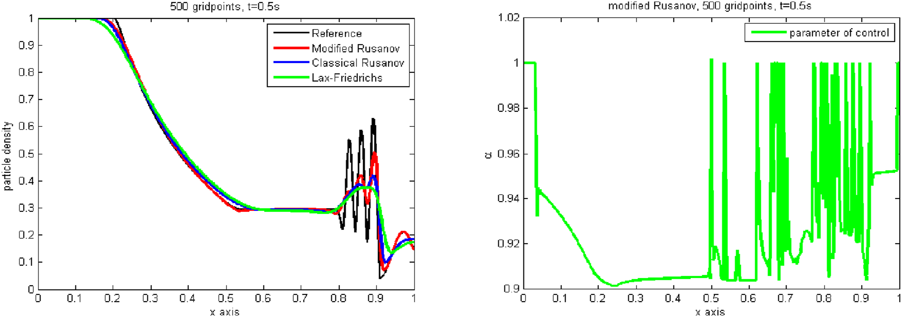
The solution involves a shock shifting from right to left and a wave of rarefaction moving from left to right. Figures 9 and 10 illustrate the pressure, velocity, particle density, and control parameter variation, respectively.

Figure 9.

Pressure, velocity at t = 0.5 s.

Figure 10.

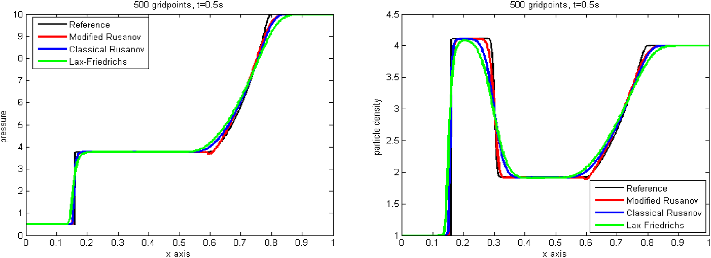
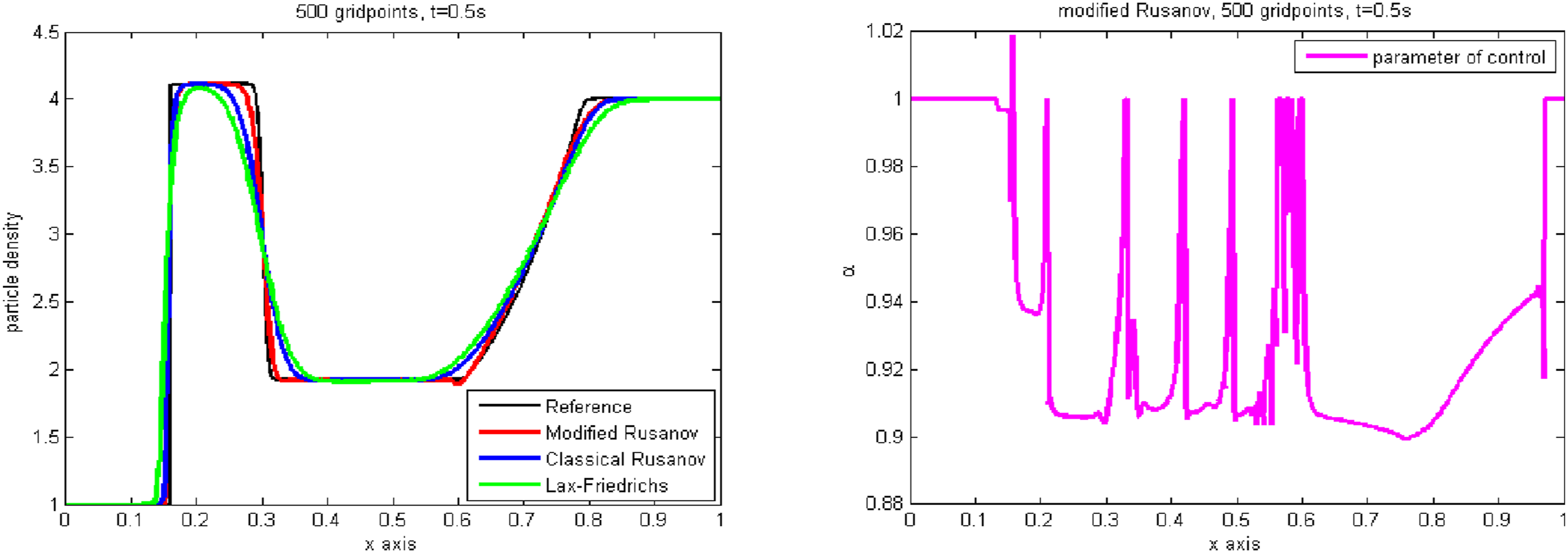
Particle density, controlling parameter ${\alpha }_{i+1/2}^n$ at time t = 0.5 s.

Sixth test

The present test case has the following initial data:

$(\mathfrak{p},\mathfrak{u},\mathfrak{n})=\left\{\begin{array}{c}(1.0,\mathrm{0,1.0})ifx\le \frac{L}{2},\hfill \\ (0.4,\mathrm{0,0.125}-0.0875\sin (50(x-0.5)))ifx>\frac{L}{2},\hfill \\ \hfill \end{array}\right.$

(4.7)

The solution is composed of wave rarefaction traveling from right to left and a shock wave traveling to the right. Figures 11 and 12 illustrate the pressure, velocity, particle density, and distinctions in control parameters, respectively.

Figure 11.

Pressure, velocity at t = 0.5 s.

Figure 12.

Particle density, controlling parameter 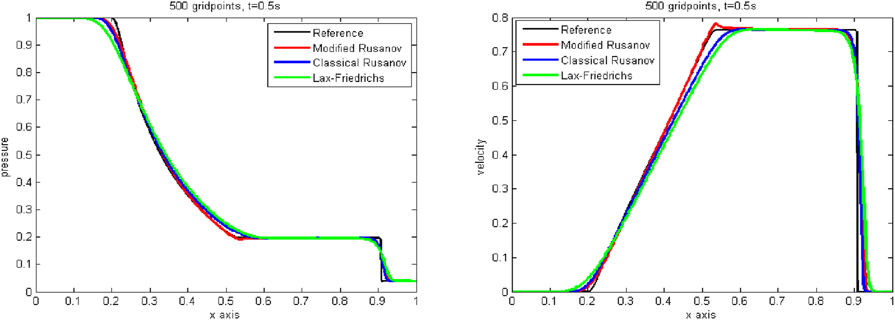${\alpha }_{i+1/2}^n$ at time t = 0.5 s.

Seventh test

The following are the initial conditions in the present case:

$(\mathfrak{p},\mathfrak{u},\mathfrak{n})=\left\{\begin{array}{c}(\mathrm{1,0,3})ifx\le \frac{L}{2},\hfill \\ (\mathrm{4,0,1})ifx>\frac{L}{2},\hfill \end{array}\right.$

(4.8)

The solution consists of wave shock going to left and a wave of rarefaction going to right. Figures 13 and 14 illustrate the pressure, velocity, particle density, and variation of parameter of control, respectively.

Figure 13.

Pressure, velocity at t = 0.5 s.

Figure 14.

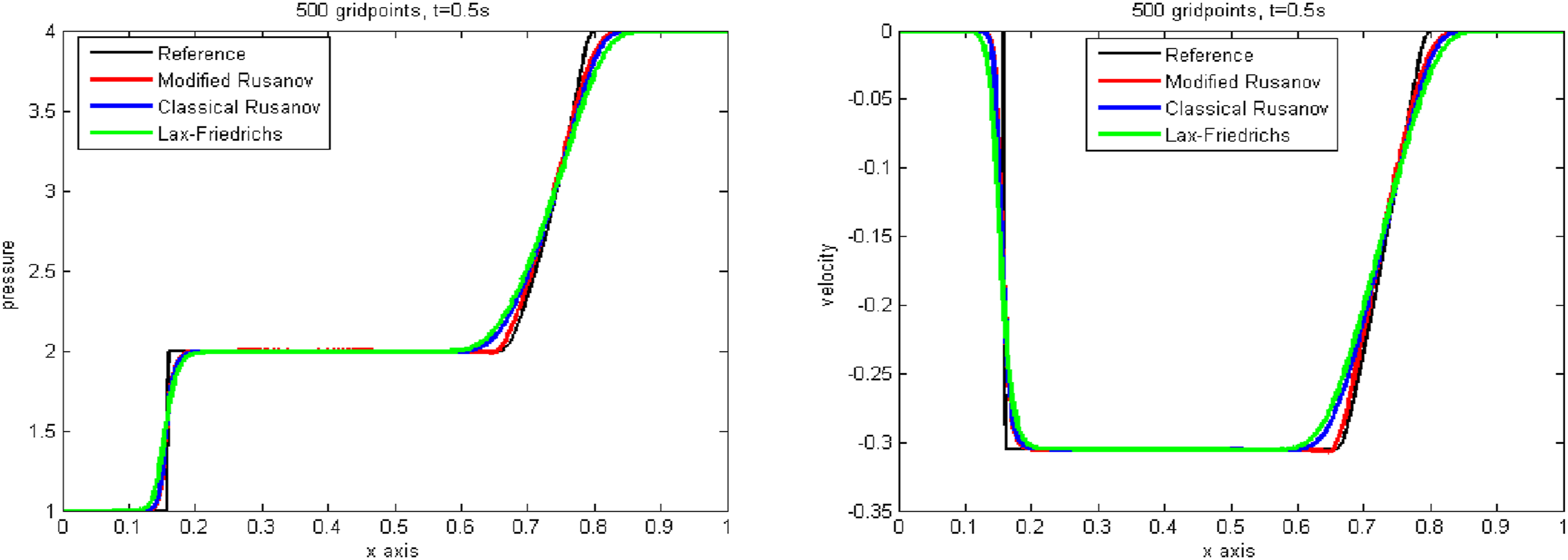
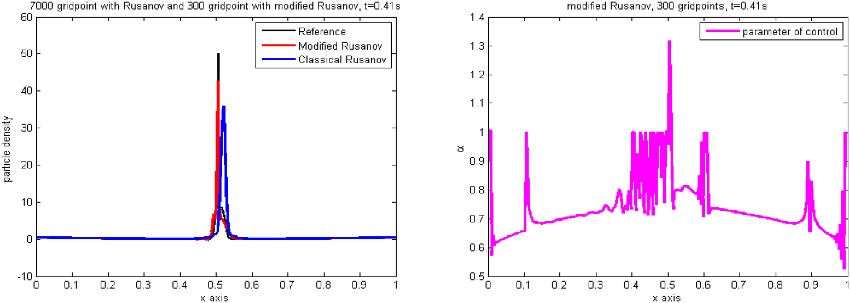
Particle density, controlling parameter ${\alpha }_{i+1/2}^n$ at t = 0.5 s.

Eighth test

This test scenario makes use of the following as its initial conditions

$(\mathfrak{p},\mathfrak{u},\mathfrak{n})=\left\{\begin{array}{c}(\mathrm{1000,0,1})if0\le x\le 0.1,\hfill \\ (0.1,\mathrm{0,1})if0.1<x\le 0.9,\hfill \\ (\mathrm{100,0,1})if0.9<x\le 1.0.\hfill \end{array}\right.$

(4.9)

The solution is constructed from up of two interfering relativistic blast waves. The numerical results on 300 mesh points for modified Rusanov and 7000 mesh points for classical Rusanov are shown in Figures 15 and 16 with final time of computation is t = 0.41 s. These figures illustrate the pressure, velocity, particle density and altering the controlling parameter, respectively. Our notice that the mR method with 300 mesh gridpoints is comparable with traditional Rusanov scheme with 7000 mesh elements.

Figure 15.

Pressure, velocity at t = 0.41 s.

Figure 16.

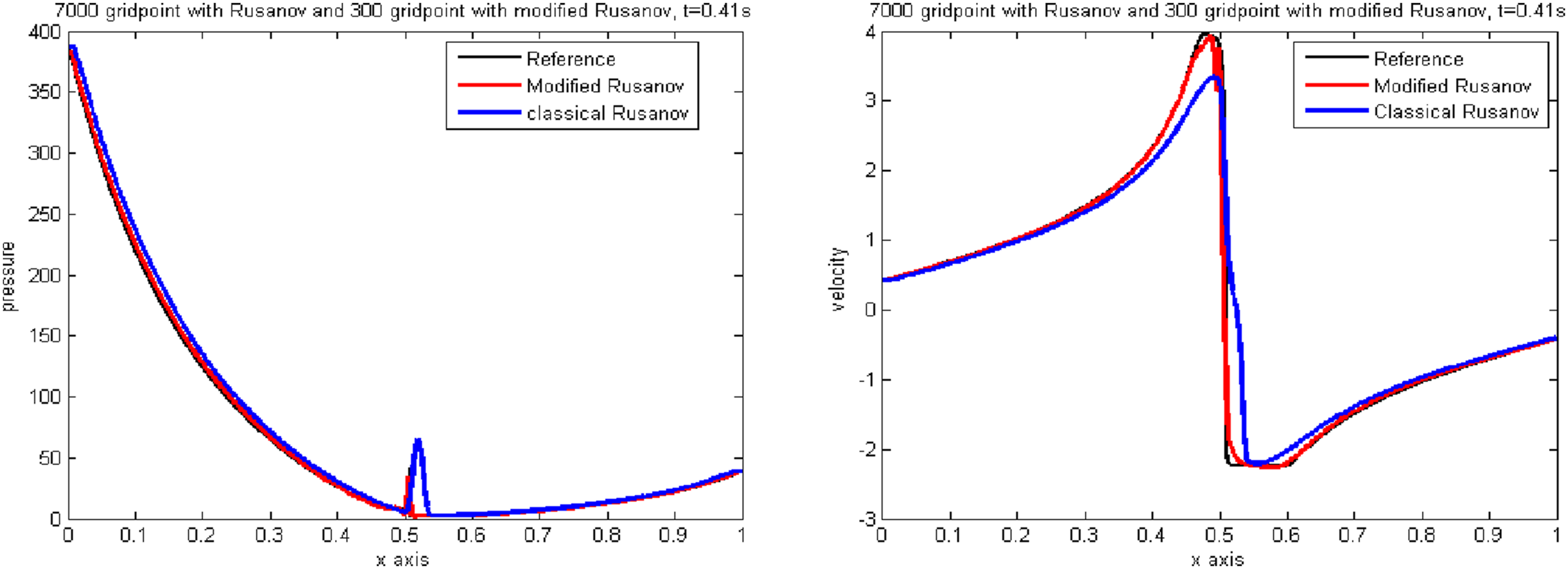
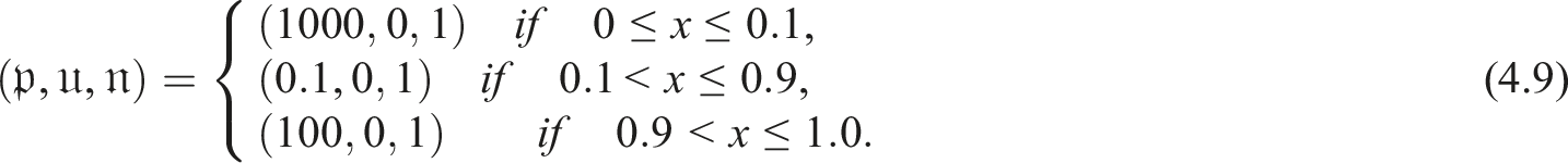
Particle density, parameter of control ${\alpha }_{i+1/2}^n$ at t = 0.41 s.

Ninth test

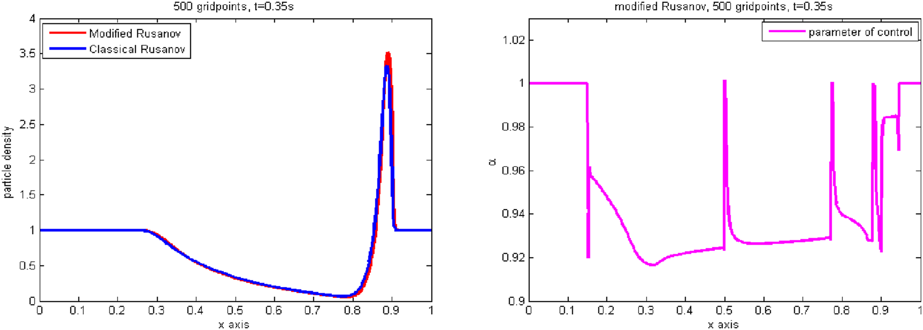
In this case, the following are the initial conditions:

$(\mathfrak{p},\mathfrak{u},\mathfrak{n})=\left\{\begin{array}{c}(\mathrm{1000,0,1})ifx\le \frac{L}{2},\hfill \\ (0.01,\mathrm{0,1})ifx>\frac{L}{2}.\hfill \end{array}\right.$

(4.10)

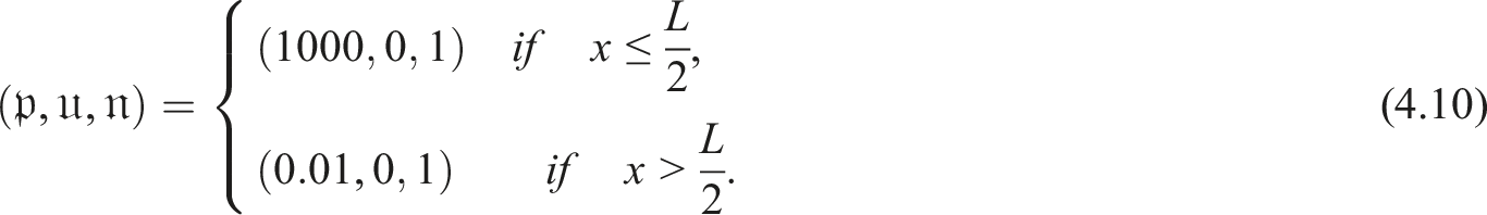
We simulate the proposed scheme and Rusanov scheme within the computation domain [0, 1] with 500 gridpoints and a t = 0.35 final execution time. Figures 17 and 18 illustrate the pressure, velocity, particle density, and changes of a controlling parameter, respectively.

Figure 17.

Pressure, velocity at t = 0.35 s.

Figure 18.

Particle density, controlling parameter 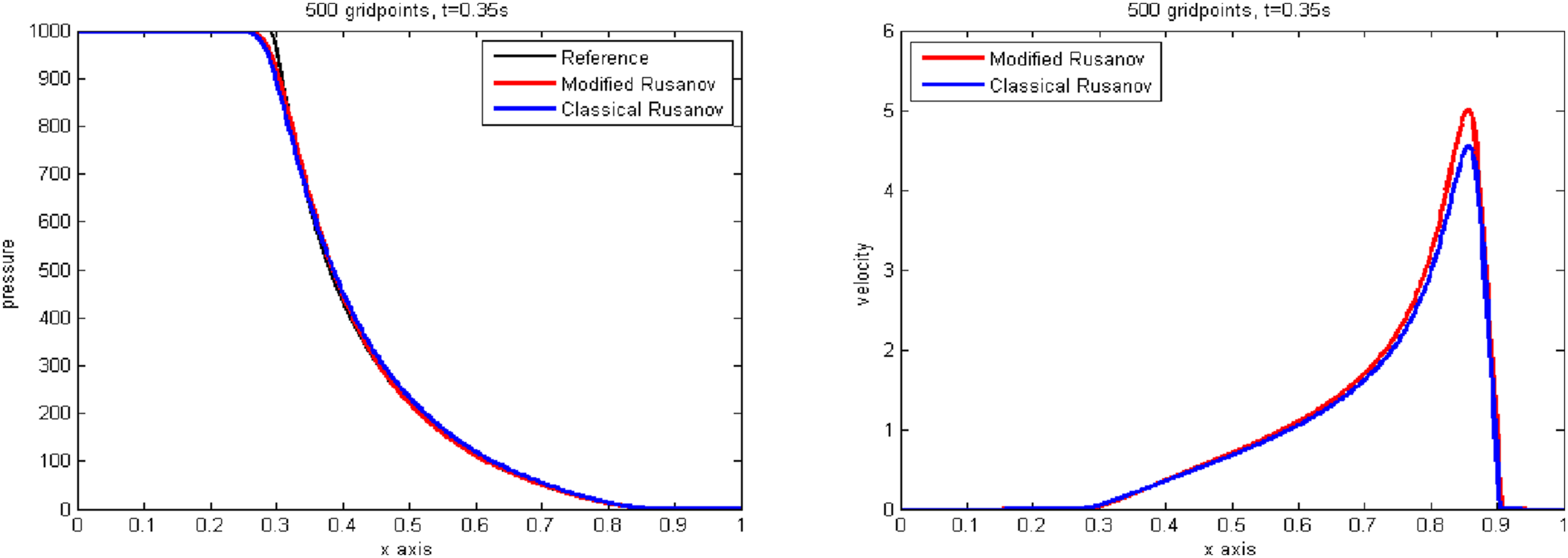${\alpha }_{i+1/2}^n$ at t = 0.35 s.

Discussion of the numerical results

We have implemented the mR scheme in order to solve the full ultra-relativistic Euler model. Actually, The basic ingredients for numerical solutions are the shock waves, contact discontinuities and rarefaction waves. The domain of computation in all calculations is [0, 1], which divides into 500 grid points, and the final computation time is t = 0.5 s, except in the test cases 4, 8, and 9, the final times are t = 0.3175 s, t = 0.41 s, and t = 0.35 s, respectively. Also, the mesh gridpoints in test case 9 is 300 mesh with modified Rusanov and 7000 mesh with traditional Rusanov scheme. We compared the pressure, velocity, and particle density results from the Rusanov, Lax-Friedrichs, and mR schemes with the reference solution that was calculated using Rusanov with 10,000 gridpoints. These techniques can all capture shock waves, contact discontinuities, and rarefaction waves. We point out that the results of the mR technique are more accurate than those of the traditional Rusanov and Lax-Friedrichs methods, with the exception of the ninth test case, where the mR scheme is equivalent to the Rusanov scheme. It was discovered that the mR scheme allows for high-resolution findings. As a result, such conservation laws can be solved numerically with accuracy and efficiency using the mR technique. Finally, the codes were built using FORTRAN 77 and the results were presented using MATLAB, this tests have been performed on 32-bit Windows7 machine with intel Core I5-2520M CPU 2.5 GHz processor.

Conclusions

In this study, we used the mR technique to solve the URE equations. Compared to well-known schemes like the Rusanov and Lax-Friedrichs schemes, this method is of the first order depending on the strength of the change in the flow and of the second order if the flow is smooth. Nine test cases are introduced to illustrate different structure of solutions for the URE model. Namely, we show the dynamical behavior of the presented solutions. According to the numerical results, the method has high precision shock and rarefaction resolution in the smooth zone and no nonphysical oscillations close to the shock locations. Therefore, it can be said that the mR technique is a reliable and efficient way to deal with these conservation law problems.

Despite this achievement, the URE model is still in its early stages of development. Future work will take into account the more practical approach of creating a new conserved scheme for the 2D URE model. Lastly, we want to expand the modified Rusanov technique to other hyperbolic PDEs, such the traffic flow model and the Euler system with changing cross-sectional area.