Stabilizing local boundary conditions for two-dimensional shallow water equations

Abstract

In this article, we present a sub-critical two-dimensional shallow water flow regulation. From the energy estimate of a set of one-dimensional boundary stabilization problems, we obtain a set of polynomial equations with respect to the boundary values as a requirement for the energy decrease. Using the Riemann invariant analysis, we build stabilizing local boundary conditions that guarantee the stability of the hydrodynamical state around a given steady state. Numerical results for the controller applied to the nonlinear problem demonstrate the performance of the method.

Introduction

Controlling the water levels and flows in river and dams is of a considerable societal interest, and it is the subject of much research in river engineering and control theory. Several control models have been developed to regulate the one-dimensional (1D) water flow. For instance, an algebraic Faedo–Galerkin method is proposed by Sene et al. ¹ where the design of a feedback control law is such that the energy decreases exponentially. The 1D flow regulation has also been addressed by the Riemann invariant analysis.^2–6 This comes out with a control law exercised on the flow through the upstream and/or downstream boundaries. To date, the extension to the two-dimensional (2D) setting has been limited in a restrictive manner. For example, a global H² stability result for a particular parabolic profile is achieved by Aamo et al. ⁷ and Balogh et al. ⁸ for the 2D Navier–Stokes equations. The authors use the actuators and the sensors only at the boundary wall. Also, under geometrical requirements, a local explicit feedback boundary control law is presented by Dia and Oppelstrup ⁹ for the stability in L²-norm of the 2D shallow water equations (SWE).

This article addresses the design and the implementation of local feedback boundary conditions that stabilize 2D shallow flow. The control’s objective is to bring the water volume to a desired steady state as fast as possible and it is subjected to the proper choice of a time-dependent boundary function called action. The implementation of such control law requires only the measurement of the initial state. The fluid movement is modeled by the SWE and is supposed to be sub-critical at the equilibrium set; hence, the well-posedness of the associated initial boundary-value problem requires two boundary conditions on the inflow boundaries and one condition on the outflow boundaries or impermeable boundaries. Considering that the controlled portion is an inflow boundary, the problem task is that of filling a bathtub with specified normal flow at the uncontrolled boundary part. For that, we use the 1D control technique developed by Dia ¹⁰ to establish stabilizing boundary conditions for the 2D SWE. The controller building process is based on the analysis of the characteristic variables of 1D hyperbolic systems. Those 1D systems are derived from a linearized version of the 2D SWE. Indeed, the main idea of this derivation is to neglect the residual rotational motions of the perturbation state so that the physical domain (for the system governing the perturbation state) is covered by a family of lines emanating from the controlled boundary portion. Afterward, a high-resolution finite volume method is used to assess the effectiveness of the proposed control law.

The rest of the article is organized as follows. In section “Setting of the problem,” we present the stabilization problem, linearize the control system around the steady state, write out the linear model governing the perturbation state, and list the main assumptions. Section “Stabilization of a dimensional reduced problem” addresses the control building process for a 1D stabilization system. Afterward, section “Numerical simulations” focuses on the original control problem; the boundary conditions for the nonlinear problem are defined and numerical experiments are performed to illustrate how the built boundary conditions stabilize the 2D nonlinear SWE.

Setting of the problem

Governing equations

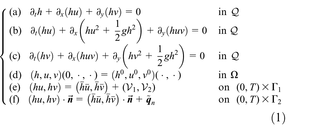
Consider a three-dimensional domain with a flat bottom in which water flows with a free-surface denoted by $\mathrm{\Omega }$ , a smooth open domain of ${\mathrm{ℝ}}^2$ , with boundary $\partial \mathrm{\Omega }={\mathrm{\Gamma }}_1\cup {\mathrm{\Gamma }}_2$ . The SWE is a set of hyperbolic partial differential equations (PDE) derived by depth integrating the Navier–Stokes equations^11,12 where one assumes that the horizontal length scale of the domain is much greater than the vertical one. In the absence of Coriolis effect, frictional, diffusion, and wind effects, the 2D SWE with boundary controller $({\mathcal{V}}_1,{\mathcal{V}}_2)$ are

$$\{\begin{array}{cc}(\mathrm{a}){\partial }_{t}h+{\partial }_x\left(\mathrm{hu}\right)+{\partial }_y\left(\mathrm{hv}\right)=0\hfill & \mathrm{in}\mathcal{Q}\hfill \\ \multicolumn{1}{c}{(\mathrm{b}){\partial }_t\left(\mathrm{hu}\right)+{\partial }_x(h{u}^2+\frac{1}{2}g{h}^2)+{\partial }_y\left(\mathrm{huv}\right)=0}& \mathrm{in}\mathcal{Q}\hfill \\ \multicolumn{1}{c}{(\mathrm{c}){\partial }_t\left(\mathrm{hv}\right)+{\partial }_x\left(\mathrm{huv}\right)+{\partial }_y(h{v}^2+\frac{1}{2}g{h}^2)=0}& \mathrm{in}\mathcal{Q}\hfill \\ \multicolumn{1}{c}{(\mathrm{d})(h,u,v)(0,·,·)=(h^0,u^0,v^0)(·,·)}& \mathrm{in}\mathrm{\Omega }\hfill \\ \multicolumn{1}{c}{(\mathrm{e})(\mathrm{hu},\mathrm{hv})=(\overline{h}\overline{u},\overline{h}\overline{v})+({\mathcal{V}}_1,{\mathcal{V}}_2)}& \mathrm{on}(0,T)\times {\mathrm{\Gamma }}_1\hfill \\ \multicolumn{1}{c}{(\mathrm{f})(\mathrm{hu},\mathrm{hv})·\overrightarrow{\mathit{n}}=(\overline{h}\overline{u},\overline{h}\overline{v})·\overrightarrow{\mathit{n}}+{\tilde{\mathit{q}}}_n}& \mathrm{on}(0,T)\times {\mathrm{\Gamma }}_2\hfill \end{array}$$

(1)

where $\mathcal{Q}=(0,T)\times \mathrm{\Omega }$ , $T>0$ , in the equations, $h$ is the height of the water column, $(u,v)$ is the velocity vector with reference to $(\mathrm{Ox},\mathrm{Oy})$ , and $g$ is the acceleration due to the gravity. The vector $\overrightarrow{\mathbf{n}}$ is the external normal vector at the boundary. The steady state $\left(\overline{h},\overline{u},\overline{v}\right)$ is the target state of the stabilization process and it is the solution of the stationary problem associated with equation (1). The quantity ${\tilde{\mathbf{q}}}_n$ represents the normal flow for the residual state at the uncontrolled boundary portion ${\mathrm{\Gamma }}_2$ . The physical domain is supposed to be uniformly convex with Lipschitz boundary. With given initial state $(h^0,u^0,v^0)$ , the control’s problem aims to provide suitable boundary condition $({\mathcal{V}}_1,{\mathcal{V}}_2)$ on ${\mathrm{\Gamma }}_1$ so that the state $(h,u,v)$ converges in time towards the equilibrium set $(\overline{h},\overline{u},\overline{v})$ .

Linearization

The SWE is derived under the hypothesis of hydrostatic balance and are based on physical nonlinear principles, whereas the design of boundary control for fluid phenomena relies on linearized wave models which are appropriate for the control of small disturbance. We introduce the conservative variable vector $\mathbf{U}=(h,q_1,q_2)$ , where $(q_1,q_2)=(\mathrm{hu},\mathrm{hv})$ and is the volumetric flow vector. Thus, equations (1a), (1b), and (1c) can be recast as

$${\partial }_t\mathbf{U}+{\partial }_x\mathbf{f}(\mathbf{U})+{\partial }_y\mathbf{g}(\mathbf{U})=0\mathrm{in}\mathcal{Q}$$

(2)

where

$$\mathbf{f}(\mathbf{U})=\left[\begin{array}{c}\mathrm{hu}\hfill \\ \multicolumn{1}{c}{h{u}^2+\frac{1}{2}g{h}^2}\\ \multicolumn{1}{c}{\mathrm{huv}}\end{array}\right]\mathrm{and}\mathbf{g}(\mathbf{U})=\left[\begin{array}{c}\mathrm{hv}\hfill \\ \multicolumn{1}{c}{\mathrm{huv}}\\ \multicolumn{1}{c}{h{v}^2+\frac{1}{2}g{h}^2}\end{array}\right]$$

Considering that the control’s objective is to reach the steady state, we introduce the residual state $\tilde{\mathbf{U}}=(\tilde{h},{\tilde{q}}_1,{\tilde{q}}_2)$ as the difference between the present state $\mathbf{U}$ and the steady state $\overline{\mathbf{U}}=(\overline{h},{\overline{q}}_1,{\overline{q}}_2)$

$$(\tilde{h},{\tilde{q}}_1,{\tilde{q}}_2)(t,x,y)=(h,q_1,q_2)(t,x,y)-(\overline{h},{\overline{q}}_1,{\overline{q}}_2)$$

Linearizing equation (1) around the steady state produces the linearized model

$${\partial }_t\tilde{\mathbf{U}}+\mathbf{A}{\partial }_x\tilde{\mathbf{U}}+\mathbf{B}{\partial }_y\tilde{\mathbf{U}}=0\mathrm{in}\mathcal{Q}$$

(3)

where

$$\begin{array}{c}\mathbf{A}=\left(\begin{array}{ccc}0\hfill & 1\hfill & 0\hfill \\ \multicolumn{1}{c}{c^2-{\overline{u}}^2}& 2\overline{u}\hfill & 0\hfill \\ \multicolumn{1}{c}{-\overline{u}\overline{v}}& \overline{v}\hfill & \overline{u}\hfill \end{array}\right)\mathrm{and}\hfill \\ \mathbf{B}=\left(\begin{array}{ccc}0\hfill & 0\hfill & 1\hfill \\ \multicolumn{1}{c}{-\overline{u}\overline{v}}& \overline{v}\hfill & \overline{u}\hfill \\ \multicolumn{1}{c}{c^2-{\overline{v}}^2}& 0\hfill & 2\overline{v}\hfill \end{array}\right)\mathrm{with}c=\sqrt{g\overline{h}}\hfill \end{array}$$

In the next subsection, the control problem (1) will be written as a stabilization problem of the above linearized system around $(0,0,0)$ .

Linearized boundary control problem

Equation (3) supports three families of wave solutions and the linearization changes dispersion forces but conserves energy of the wave field. The stabilization of equation (1) (reach the steady state) around $(\overline{h},{\overline{q}}_1,{\overline{q}}_2)$ has been replaced by the stabilization of equation (4) (cancel perturbation) around $(0,0,0)$ with prescribed initial conditions. Therefore, our control’s objective is now to find a boundary controller $({\mathcal{V}}_1,{\mathcal{V}}_2)$ on ${\mathrm{\Gamma }}_1$ , that is, boundary conditions to apply there, so that $(\tilde{h},{\tilde{q}}_1,{\tilde{q}}_2)$ is stable around $(0,0,0)$ . For that, we consider the linearized control problem

$$\{\begin{array}{cc}(\mathrm{a}){\partial }_t\tilde{\mathbf{U}}+\mathbf{A}{\partial }_x\tilde{\mathbf{U}}+\mathbf{B}{\partial }_y\tilde{\mathbf{U}}=0\hfill & \mathrm{in}\mathcal{Q}\hfill \\ \multicolumn{1}{c}{(\mathrm{b})(\tilde{h},{\tilde{q}}_1,{\tilde{q}}_2)(0,·,·)=({\tilde{h}}^0,{\tilde{q}}_1^0,{\tilde{q}}_2^0)(·,·)}& \mathrm{in}\mathrm{\Omega }\hfill \\ \multicolumn{1}{c}{(\mathrm{c})({\tilde{q}}_1,{\tilde{q}}_2)=({\mathcal{V}}_1,{\mathcal{V}}_2)}& \mathrm{on}(0,T)\times {\mathrm{\Gamma }}_1\hfill \\ \multicolumn{1}{c}{(\mathrm{d})({\tilde{q}}_1,{\tilde{q}}_2)·\overrightarrow{n}={\tilde{\mathbf{q}}}_n}& \mathrm{on}(0,T)\times {\mathrm{\Gamma }}_2\hfill \end{array}$$

(4)

Classical boundary conditions such as wall condition, periodic boundary conditions, and absorbing boundary conditions could be set to the system (4). However, we seek for boundary conditions that also give well-posed initial boundary-value problem (IBVP) and are able to bring the state $(\tilde{h},{\tilde{q}}_1,{\tilde{q}}_2)$ to $(0,0,0)$ as fast as possible.

It is worth noting that equation (4) is a well-posed IBVP; see the construction of admissible boundary conditions^9,13 for more details. In the next subsection, we list the assumptions to delineate the frame of the building process of the boundary controller.

Assumptions for the boundary conditions design

In this subsection, we list the assumptions and define the plan of the building process of the boundary conditions $({\mathcal{V}}_1,{\mathcal{V}}_2)$ :

• A1: To keep the building process of the stabilizing boundary conditions as simple as possible, we restrict our study to uniform steady states, but this is not necessary for the derivation of equation (4). A typical case of an application where this argument rests is the flow regulation of a river/lake with navigability constraints (regulation of the Sambre river and the Meuse river in France and Belgium by Bastin et al. ¹⁴ ). Linearization around non-uniform steady state provides variable Jacobian matrices and is outside the scope of this article. A method for the design of local boundary conditions that stabilize 2D SWE around a non-uniform equilibrium will be discussed in a forthcoming paper.

• A2: We deal with the sub-critical flow regime. Accordingly, we specify the flow vector at inflow (i.e. on ${\mathrm{\Gamma }}_1$ ) and prescribe the normal flow rate through the boundary part ${\mathrm{\Gamma }}_2$ .^15,16 In others words, to define the boundary conditions (4c) and (4d), we only need to design $({\mathcal{V}}_1,{\mathcal{V}}_2)$ . The normal flow ${\tilde{\mathbf{q}}}_n$ at equation (4d) is a reflecting boundary condition for the gravity waves on the uncontrolled boundary portion ${\mathrm{\Gamma }}_2$ , and it will be computed according to the control law on ${\mathrm{\Gamma }}_1$ .

  The assumption of the sub-critical flow regime also implies that the values $\overline{h},\overline{u}$ and $\overline{v}$ of the equilibrium state are non-zero, and the Froude number $F_r$ satisfies $F_r=\frac{{\Vert (\overline{u},\overline{v})\Vert }_2}{c}<1$ . For the sake of simplicity, we consider $\overline{u}$ and $\overline{v}$ positive, especially in the numerical experiments.

• A3: We deal with a uniform convex domain $\mathrm{\Omega }$ with Lipschitz boundary $\partial \mathrm{\Omega }={\mathrm{\Gamma }}_1\cup {\mathrm{\Gamma }}_2$ . We denote by $\phi$ the viewing angle of the controlled boundary portion ${\mathrm{\Gamma }}_1$ , and $\theta$ the angle between the x-axis and the straight line $(D_{\theta })$ . The latter passes through $O$ and intersects the boundary at points $L_{1_{\theta }}$ and $L_{2_{\theta }}$ with $L_{1_{\theta }}\in {\mathrm{\Gamma }}_1$ and $L_{2_{\theta }}\in {\mathrm{\Gamma }}_2$ as illustrated in Figure 1.

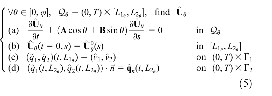
• A4: Under the assumption of flow irrotationality, we move from the Cartesian coordinates $(x,y)$ to the specific family of lines $s=x\cos \theta +y\sin \theta$ , where $\theta =\arctan \left(\frac{y}{x}\right)$ . We then make the reduction in the domain dimension from 2D to 1D by disregarding the $\theta$ -dependence of $\tilde{\mathbf{U}}$ . Let ${\overrightarrow{\mathit{n}}}_{\theta }$ be the unit vector of components $(\cos \theta ,\sin \theta )$ along $(D_{\theta })$ . We use the notation ${\hat{\mathbf{U}}}_{\theta }(t,s)$ for the approximation of the residual state $\tilde{\mathbf{U}}(t,x,y)$ over the line $(D_{\theta })$ . Projection of the 2D equations (4) onto the lines produces a set of 1D hyperbolic problems

$$\{\begin{array}{c}\forall \theta \in [0,\phi ],{\mathcal{Q}}_{\theta }=(0,T)\times [L_{1_{\theta }},L_{2_{\theta }}],\mathrm{find}{\hat{\mathbf{U}}}_{\theta }\hfill \\ \multicolumn{1}{c}{(\mathrm{a})\frac{\partial {\hat{\mathbf{U}}}_{\theta }}{\partial t}+(\mathbf{A}\cos \theta +\mathbf{B}\sin \theta )\frac{\partial {\hat{\mathbf{U}}}_{\theta }}{\partial s}=0}& \mathrm{in}{\mathcal{Q}}_{\theta }\hfill \\ \multicolumn{1}{c}{(\mathrm{b}){\hat{\mathbf{U}}}_{\theta }(t=0,s)={\hat{\mathbf{U}}}_{\theta }^0(s)}& \mathrm{in}[L_{1_{\theta }},L_{2_{\theta }}]\hfill \\ \multicolumn{1}{c}{(\mathrm{c})({\hat{q}}_1,{\hat{q}}_2)(t,L_{1_{\theta }})=({\hat{v}}_1,{\hat{v}}_2)}& \mathrm{on}(0,T)\times {\mathrm{\Gamma }}_1\hfill \\ \multicolumn{1}{c}{(\mathrm{d})({\hat{q}}_1(t,L_{2_{\theta }}),{\hat{q}}_2(t,L_{2_{\theta }}))·\overrightarrow{n}={\hat{\mathbf{q}}}_n(t,L_{2_{\theta }})}& \mathrm{on}(0,T)\times {\mathrm{\Gamma }}_2\hfill \end{array}$$

(5)

Although the system (5) varies with the plane-polar coordinates $(s,\theta )$ , it describes the disregarding of $\theta$ of the linearized model (4) but it is not standing for the linearized version of the polar coordinates SWE,^17,18 since we drop the terms $\frac{1}{s}\frac{\partial \tilde{\mathbf{U}}}{\partial \theta }\frac{\partial (\mathbf{A}\cos \theta +\mathbf{B}\sin \theta )}{\partial \theta }$ . This transformation concerns only the design of the boundary conditions but not for the control system. Therefore, it is crucial to note that the irrotational assumption is restricted to the perturbation state and only for the purpose of building local boundary conditions.

It is then adequate using equation (5) to analyze the wave dynamics. Indeed, the regularity is conserved through equation (5) since the system (4a) is strictly hyperbolic ¹⁹ —A4 leads to the uncoupling of the controlled portion of the boundary so that controlling one point on ${\mathrm{\Gamma }}_1$ can be done using only two points which are aligned along a ray. The singular value decomposition of the flux matrices of the polar coordinates of 2D SWE with $\overline{u},\overline{v}>0$ combined with the absence of Coriolis effects reveals an important dominance of the term $(\mathbf{A}\cos \theta +\mathbf{B}\sin \theta )\frac{\partial {\hat{\mathbf{U}}}_{\theta }}{\partial s}$ .

The shallow water gravity waves governed by system (5) obey unidirectional radial dispersions. Hence, they allow us to analyze the flow over a specific family of lines. To build stabilizing conditions, a flux analysis will be carried out by considering ${\hat{\mathbf{U}}}_{\theta }=(\hat{h},{\hat{q}}_1,{\hat{q}}_2)$ . In the next section, we present the design of stabilizing boundary conditions for equation (5) for a fixed $\theta$ .

Figure 1.

Schema of the domain $\mathrm{\Omega }$ treatment with controlled boundary portion ${\mathrm{\Gamma }}_1$ and uncontrolled boundary part ${\mathrm{\Gamma }}_2$ .

Stabilization of a dimensional reduced problem

So far, we have written the control problem (1) in terms of cancelation of the perturbation state and have derived a set of 1D control problems. In this section, a stabilization result of the reduced 1D problem is presented. Consequently, the control $({\hat{v}}_1(t,L_{1_{\theta }}),{\hat{v}}_2(t,L_{1_{\theta }}))$ and the normal flow ${\hat{\mathbf{q}}}_n(t,L_{2_{\theta }})$ will be designed using only the upstream boundary information, as described by Dia. ¹⁰

Characteristic variables

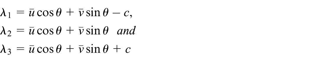
The eigenvalues (phase speeds) ${\lambda }_i$ of the matrix $\mathbf{A}\cos \theta +\mathbf{B}\sin \theta$ are

$$\begin{array}{l}{\lambda }_1=\overline{u}\cos \theta +\overline{v}\sin \theta -c,\\ {\lambda }_2=\overline{u}\cos \theta +\overline{v}\sin \theta and\\ {\lambda }_3=\overline{u}\cos \theta +\overline{v}\sin \theta +c\end{array}$$

Let $\mathbf{\Lambda }$ and $\mathbf{P}$ be, respectively, the diagonal matrix of eigenvalues and the matrix of eigenvectors of $\mathbf{A}\cos \theta +\mathbf{B}\sin \theta$ , then $\mathbf{A}\cos \theta +\mathbf{B}\sin \theta =\mathbf{P}\mathbf{\Lambda }{\mathbf{P}}^{-1}$ where

$$\mathbf{P}=\left(\begin{array}{ccc}1\hfill & 0\hfill & 1\hfill \\ \multicolumn{1}{c}{\overline{u}-c\cos \theta }& -\sin \theta \hfill & \overline{u}+c\cos \theta \hfill \\ \multicolumn{1}{c}{\overline{v}-c\sin \theta }& \cos \theta \hfill & \overline{v}+c\sin \theta \hfill \end{array}\right)$$

and $\mathbf{\Lambda }=\mathrm{diag}\{{\lambda }_1,{\lambda }_2,{\lambda }_3\}$ . After multiplication from left of $\frac{\partial {\hat{\mathbf{U}}}_{\theta }}{\partial t}+\mathbf{P}\mathbf{\Lambda }{\mathbf{P}}^{-1}\frac{{\hat{\mathbf{U}}}_{\mathbf{\theta }}}{\partial \mathbf{s}}=0$ by ${\mathbf{P}}^{-1}$ , it appears

$${\partial }_t\mathit{\xi }(t,s)+\mathbf{\Lambda }{\partial }_s\mathit{\xi }(t,s)=0$$

(6)

where $\mathit{\xi }(t,s)=({\xi }_1,{\xi }_2,{\xi }_3{)}^{\mathrm{tr}}={\mathbf{P}}^{-1}{\hat{\mathbf{U}}}_{\mathbf{\theta }}$ . The Riemann invariants (normal modes) ${\xi }_i$ for $i=1,2,3$ can be written out in details

$${\xi }_1(t,s)=\frac{1}{2c}({\lambda }_3\hat{h}(t,s)-Q_1(t,s)),Q_1(t,s)=\cos \theta {\hat{q}}_1(t,s)+\sin \theta {\hat{q}}_2(t,s)$$

(7)

$${\xi }_2(t,s)=\lambda {\prime }_2\hat{h}(t,s)+Q_2(t,s),Q_2(t,s)=\cos \theta {\hat{q}}_2(t,s)-\sin \theta {\hat{q}}_1(t,s)$$

(8)

$${\xi }_3(t,s)=\frac{1}{2c}(-{\lambda }_1\hat{h}(t,s)+Q_1(t,s)),{\lambda }_{2\prime }=\overline{u}\sin \theta -\overline{v}\cos \theta$$

(9)

The quantities $Q_1$ and $Q_2$ are viewed as volumetric flow variables over the line $(D_{\theta })$ . The sub-critical regime implies that $\sqrt{{\overline{u}}^2+{\overline{v}}^2}<c$ and that there are gravity waves (waves with velocities ${\lambda }_1$ and ${\lambda }_3$ ) propagating in opposite directions. It follows that ${\lambda }_1<0$ and ${\lambda }_3>0$ while the sign of ${\lambda }_2$ is not known in advance since it depends on $\theta$ . In fact, the sign of ${\lambda }_2$ determines the flow direction over the line $(L_{1_{\theta }}{L}_{2_{\theta }})$ . Choosing ${\lambda }_2>0\forall \theta \in [0,\phi ]$ corresponds to a regime with inflow at the boundary ${\mathrm{\Gamma }}_1$ . The domain description (assumption A3) ensures that and sets the reference $(O,\mathrm{Ox},\mathrm{Oy})$ such that ${\lambda }_2>0$ for a given steady state and for all $\theta \in [0,\phi ]$ .

Boundary controller building process

For a fixed value of $\theta$ , we denote $T_{\theta }=\frac{L_{2_{\theta }}-L_{1_{\theta }}}{{\lambda }_3}$ and consider the 1D stabilization problem for a channel flow controlled by one gate opening using an upstream boundary control over $(D_{\theta })$ as depicted in Figure 2.

Figure 2.

Lateral view of the reduced one-dimensional domain with upstream boundary control action.

To build the stabilizing boundary condition for the control problem (5), we consider the eigenstructure system

$$\{\begin{array}{cc}{\partial }_t\mathit{\xi }(t,s)+\mathbf{\Lambda }{\partial }_s\mathit{\xi }(t,s)=0\hfill & \mathrm{in}{\mathcal{Q}}_{\theta },\hfill \\ \multicolumn{1}{c}{\mathit{\xi }(t=0,s)={\mathit{\xi }}^0(s)}& \mathrm{in}[L_{1_{\theta }},L_{2_{\theta }}]\hfill \\ \multicolumn{1}{c}{{\xi }_1(t,L_{2_{\theta }})=\{\begin{array}{c}(\frac{{\lambda }_3}{-{\lambda }_1}{\xi }_3^0(L_{1_{\theta }})-{\xi }_1^0(L_{2_{\theta }}))\frac{t}{T_{\theta }}+{\xi }_1^0(L_{2_{\theta }})\mathrm{in}[0,T_{\theta }]\hfill \\ \multicolumn{1}{c}{\frac{{\lambda }_3}{-{\lambda }_1}{\alpha }_{\theta }(t-T_{\theta })\mathrm{in}[T_{\theta },T]}\end{array}}\\ \multicolumn{1}{c}{{\xi }_2(t,L_{1_{\theta }})=K(\kappa ){\alpha }_{\theta }(t)}& \mathrm{in}[0,T]\hfill \\ \multicolumn{1}{c}{{\xi }_3(t,L_{1_{\theta }})={\alpha }_{\theta }(t)}& \mathrm{in}[0,T]\hfill \end{array}$$

(10)

where the time-dependent function ${\alpha }_{\theta }$ defined in $[0,+\infty )$ stands for the upstream boundary action and the parameter $\kappa$ is chosen with respect to the gravity velocities, the stabilization rate $\mu$ , and the initial condition ${\mathit{\xi }}^0$ . Functions ${\alpha }_{\theta }$ and $K(\kappa )$ will be defined, and the boundary conditions ${\xi }_1(t,L_{2_{\theta }})$ and ${\xi }_2(t,L_{1_{\theta }})$ for $0\le t\le T_{\theta }$ will be justified.

Definition 1

For all fixed $\theta \in [0,\phi ]$ , we consider the following energy of (10)

$$E_{\theta }(t)=\sum _{i=1}^3{\int }_{L_{1_{\theta }}}^{L_{2_{\theta }}}{\xi }_i^2(t,s)\exp (-\frac{\mu }{{\lambda }_i}s)\mathrm{ds}$$

(11)

where $\mu$ is an arbitrary positive number.

This is the quantity to be stabilized and $\mu$ represents the stabilization rate. This definition shows that the energy can only change according to the changes of $\mathbf{\xi }$ across the boundaries. The weighting term in equation (11) makes sense since ${\lambda }_i\ne 0$ for $i=1,2,3$ as guaranteed by the physical domain description (assumption A3).

Let us remark that the hyperbolic equation (10) can be controlled performing output feedback force ²⁰ on the energy quantity (11).

Dissipative boundary conditions

For $i=1,2,3$ , one integrates on $[L_{1_{\theta }},L_{2_{\theta }}]$ the product of $\frac{\partial {\xi }_i}{\partial t}(t,s)+{\lambda }_i\frac{\partial {\xi }_i}{\partial s}(t,s)=0$ by ${\xi }_i(t,s)\exp (-\frac{\mu }{{\lambda }_i}s)$ and sums the three obtained relations to write the following energy estimation

$$\frac{\partial E_{\theta }(t)}{\partial t}+\mu E_{\theta }(t)=-\sum _{i=1}^3{\lambda }_i{[{\xi }_i^2(t,s)\exp (-\frac{\mu }{{\lambda }_i}s)]}_{L_{1_{\theta }}}^{L_{2_{\theta }}}$$

(12)

Exponential decay of the energy $E_{\theta }$ is achieved when the right-hand side (RHS) of equation (12) is non-positive.

We choose an action ${\alpha }_{\theta }$ satisfying

$${\xi }_1^2(t,L_{1_{\theta }})-{\xi }_1^2(t,L_{2_{\theta }})\exp (-\mu \frac{L_{\theta }}{{\lambda }_1})\ge 0$$

(13)

$${\xi }_2^2(t,L_{1_{\theta }})-{\xi }_2^2(t,L_{2_{\theta }})\exp (-\mu \frac{L_{\theta }}{{\lambda }_2})\le 0$$

(14)

$${\xi }_3^2(t,L_{1_{\theta }})-{\xi }_3^2(t,L_{2_{\theta }})\exp (-\mu \frac{L_{\theta }}{{\lambda }_3})=0$$

(15)

where $L_{\theta }=L_{2_{\theta }}-L_{1_{\theta }}$ . The relations (13)–(15) are dissipative boundary conditions ²¹ which are a sufficient exponential stability condition for equation (10). Our idea to fulfill the stability is to define an upstream action ${\alpha }_{\theta }$ using equation (15) and then to determine the corresponding flow rates $Q_1(t,L_{1_{\theta }})$ and $Q_2(t,L_{1_{\theta }})$ by satisfying equations (13) and (14).

Definition of the boundary action

The boundary action ${\alpha }_{\theta }$ can be defined as a damping function acting on the inflow at the upstream boundary $L_{1_{\theta }}$ . To express the boundary action ${\alpha }_{\theta }$ , we consider the third characteristic equation

$$\frac{\partial {\xi }_3}{\partial t}(t,s)+{\lambda }_3\frac{\partial {\xi }_3}{\partial s}(t,s)=0$$

(16)

We integrate equation (16) over the characteristic line from $(t,L_{1_{\theta }})$ to $(t+T_{\theta },L_{2_{\theta }})$ to get

$${\xi }_3(t,L_{1_{\theta }})={\xi }_3(t+T_{\theta },L_{2_{\theta }})$$

(17)

Then, we act on the characteristic variable ${\xi }_3$ at the boundary $L_{1_{\theta }}$

$${\xi }_3(t,L_{1_{\theta }})={\alpha }_{\theta }(t)$$

(18)

where ${\alpha }_{\theta }$ is a time-dependent function. Therefore, using equation (17), we get

$${\xi }_3(t,L_{2_{\theta }})={\xi }_3(t-T_{\theta },L_{1_{\theta }})$$

(19)

$$={\alpha }_{\theta }(t-T_{\theta })\mathrm{for}t\ge T_{\theta }.$$

(20)

We can then write equation (15) as

$${\alpha }_{\theta }^2(t)-{\alpha }_{\theta }^2(t-T_{\theta })\exp (-\mu T_{\theta })=0$$

Finally, to satisfy equation (15), we have to define the action function ${\alpha }_{\theta }$ such that $\forall t\ge T_{\theta }$

$$\{\begin{array}{c}{\alpha }_{\theta }(0)={\xi }_3^0(L_{1_{\theta }})\hfill \\ \multicolumn{1}{c}{{\alpha }_{\theta }(t)={\alpha }_{\theta }(t-T_{\theta })\exp (-\mu \frac{T_{\theta }}{2})}\end{array}$$

(21)

Note that the action ${\alpha }_{\theta }$ is completely defined when it is given on $[0,T_{\theta }]$ . The control action ${\alpha }_{\theta }$ requires $T_{\theta }$ as observability time and it is being defined for $t\ge T_{\theta }$ . In the time interval $[0,T_{\theta }]$ , the function ${\alpha }_{\theta }$ can be chosen arbitrarily provided that ${\alpha }_{\theta }(0)={\xi }_3^0(L_{1_{\theta }})$ . It is arbitrary in the sense that any non-growing function can be set to it.

Boundary conditions at $L_{2_{\theta }}$ (downstream)

According to the signs of the eigenvalues, only one condition should be stood at this boundary; we deal with

$$Q_1(t,L_{2_{\theta }})=0$$

(22)

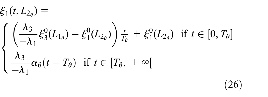
This condition reflects the gravity waves ( ${\xi }_1$ and ${\xi }_3$ ) and can be written as

$${\xi }_1(t,L_{2_{\theta }})=\frac{{\lambda }_3}{-{\lambda }_1}{\alpha }_{\theta }(t-T_{\theta })\forall t\ge T_{\theta }$$

(23)

This last characteristic decomposition reveals that boundary condition (22) for ${\xi }_1$ on $[0,T_{\theta }]$ is not yet defined, because for $t\in [0,T_{\theta }]$ , the function ${\alpha }_{\theta }$ is not acting on the characteristic variables ${\xi }_1$ and ${\xi }_2$ but only on the characteristic variable ${\xi }_3$ since it is being defined. To fill that gap, we consider the fact that ${\xi }_1(T_{\theta },L_{2_{\theta }})$ can be written out at the initial time $(t=0)$

$${\xi }_1(T_{\theta },L_{2_{\theta }})=\frac{{\lambda }_3}{-{\lambda }_1}{\alpha }_{\theta }(0)=\frac{{\lambda }_3}{-{\lambda }_1}{\xi }_3^0(L_{1_{\theta }})$$

(24)

and we use the following linear mapping; $\forall 0\le t\le T_{\theta }$

$${\xi }_1(t,L_{2_{\theta }})=\frac{\frac{{\lambda }_3}{-{\lambda }_1}{\xi }_3^0(L_{1_{\theta }})-{\xi }_1^0(L_{2_{\theta }})}{T_{\theta }}t+{\xi }_1^0(L_{2_{\theta }})$$

(25)

The boundary condition at the downstream boundary is then given by

$$\begin{array}{c}{\xi }_1(t,L_{2_{\theta }})=\hfill \\ \{\begin{array}{c}(\frac{{\lambda }_3}{-{\lambda }_1}{\xi }_3^0(L_{1_{\theta }})-{\xi }_1^0(L_{2_{\theta }}))\frac{t}{T_{\theta }}+{\xi }_1^0(L_{2_{\theta }})\mathrm{if}t\in [0,T_{\theta }]\hfill \\ \multicolumn{1}{c}{\frac{{\lambda }_3}{-{\lambda }_1}{\alpha }_{\theta }(t-T_{\theta })\mathrm{if}t\in [T_{\theta },+\infty [}\end{array}\hfill \end{array}$$

(26)

Boundary conditions at $L_{1_{\theta }}$ (upstream boundary controller)

The conditions at $L_{1_{\theta }}$ are completely defined by the prescription of the flow $(Q_1(t,L_{1_{\theta }}),Q_2(t,L_{1_{\theta }}))$ . We get those quantities by writing equations (13) and (14) as two second-order inequalities with respect to $Q_1(t,L_{1_{\theta }})$ and $Q_2(t,L_{1_{\theta }})$ , respectively. To replace $\hat{h}(t,L_{1_{\theta }})$ and $\hat{h}(t,L_{2_{\theta }})$ in the inequalities, one uses equations (17) and (18) and condition (22) to write: for $t\ge T_{\theta }$

$$\begin{array}{c}\hat{h}(t,L_{1_{\theta }})=\frac{1}{{\lambda }_1}(Q_1(t,L_{1_{\theta }})-2c{\alpha }_{\theta }(t))\mathrm{and}\hfill \\ \hat{h}(t,L_{2_{\theta }})=\frac{2c}{-{\lambda }_1}{\alpha }_{\theta }(t-T_{\theta })\hfill \end{array}$$

(27)

Thanks to equation (27), the left-hand side (LHS) of equations (13) and (14) can be written as second-order polynomials with respect to $Q_1(t,L_{1_{\theta }})$ and $R(t,L_{1_{\theta }})=\frac{{\lambda }_{2\prime }}{{\lambda }_1}{Q}_1(t,L_{1_{\theta }})+Q_2(t,L_{1_{\theta }})$ , respectively, and whom the roots are

$$Q_{1_1}(t,L_{1_{\theta }})=\frac{1-{\sigma }_1}{2}\frac{{\lambda }_3}{c}{\alpha }_{\theta }(t),R_1(t,L_{1_{\theta }})=2\frac{c}{{\lambda }_1}(\lambda {\prime }_2+\left|\lambda {\prime }_2\right|{\sigma }_2){\alpha }_{\theta }(t)$$

$$Q_{1_2}(t,L_{1_{\theta }})=\frac{1+{\sigma }_1}{2}\frac{{\lambda }_3}{c}{\alpha }_{\theta }(t),R_2(t,L_{1_{\theta }})=2\frac{c}{{\lambda }_1}(\lambda {\prime }_2-\left|\lambda {\prime }_2\right|{\sigma }_2){\alpha }_{\theta }(t)$$

where

$${\sigma }_1^2=-3+4\exp (-2\mu \frac{T_{\theta }c}{{\lambda }_1})\mathrm{and}{\sigma }_2^2=\exp (-\mu \frac{T_{\theta }c}{{\lambda }_2})$$

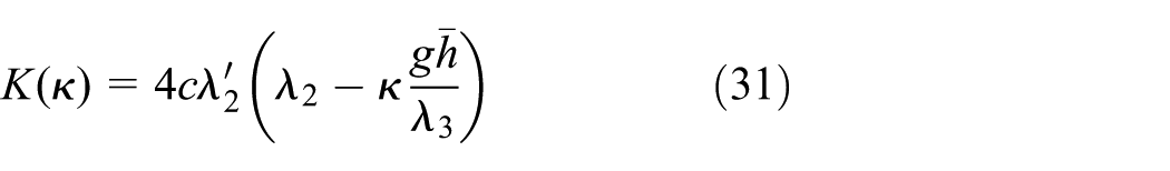
According to the coefficient of the second-order monomials, we choose the mean value of $R_1(t,L_{1_{\theta }})$ and $R_2(t,L_{1_{\theta }})$

$$R(t,L_{1_{\theta }})=2\frac{\lambda {\prime }_2}{{\lambda }_1}c{\alpha }_{\theta }(t)$$

(28)

and select

$$Q_1(t,L_{1_{\theta }})=2\kappa \frac{c}{{\lambda }_3}{\alpha }_{\theta }(t)$$

(29)

where $\kappa \in ]-\infty ,1-{\sigma }_1]\cup [1+{\sigma }_1,+\infty [$ . We can now write explicitly the boundary condition for ${\xi }_2$ at $L_{1_{\theta }}$ corresponding to the action ${\alpha }_{\theta }(t)$ for $t\ge T_{\theta }$ using characteristic variables

$${\xi }_2(t,L_{1_{\theta }})=K(\kappa ){\alpha }_{\theta }(t)\forall t\ge T_{\theta }$$

(30)

where

$$K(\kappa )=4c\lambda {\prime }_2({\lambda }_2-\kappa \frac{g\overline{h}}{{\lambda }_3})$$

(31)

As for the variable ${\xi }_1$ , the boundary condition at $L_{1_{\theta }}$ for ${\xi }_2$ on $[0,T_{\theta }]$ is not yet defined. To do so, we consider the choice of $\kappa$ such that

$$K(\kappa ){\alpha }_{\theta }(0)={\xi }_2^0(L_{1_{\theta }})$$

(32)

Such $\kappa$ exists, belongs to $]-\infty ,1-{\sigma }_1]\cup [1+{\sigma }_1,+\infty [$ and satisfies equation (32) according to the initial conditions. At $L_{1_{\theta }}$ the conditions are written as follows

$${\xi }_2(t,L_{1_{\theta }})=K(\kappa ){\alpha }_{\theta }(t)\mathrm{if}t\in [0,+\infty [$$

(33)

where $\kappa$ is such that equation (32) is satisfied

$${\xi }_3(t,L_{1_{\theta }})={\alpha }_{\theta }(t)\mathrm{if}t\in [0,+\infty [$$

(34)

We are now in the position to state our basic result for the exponential stability of a 1D hyperbolic system by means of the time-dependent action ${\alpha }_{\theta }$ .

Theorem 1

If the initial condition ${\xi }^0$ is in $L^2(L_{1_{\theta }},L_{2_{\theta }}{)}^3$ , then there exists an upstream boundary action ${\alpha }_{\theta }$ such that the stabilization system (10) has a unique global $L^2(L_{1_{\theta }},L_{2_{\theta }}{)}^3$ solution $\mathbf{\xi }$ and the following energy estimation holds

$$E_{\theta }(t)\le E_{\theta }(T_{\theta })\exp (-\mu (t-T_{\theta }))\forall t\ge T_{\theta }$$

(35)

Proof

It is well known that the unique solution $\mathbf{\xi }=({\mathbf{\xi }}_1,{\mathbf{\xi }}_2,{\mathbf{\xi }}_3)$ with the initial condition ${\mathbf{\xi }}^0$ has the form ${\xi }_i(t,s)={\xi }_i^0(s-{\lambda }_{i}t)$ for $i=1,2,3$ .

The exponential decay of the energy $E_{\theta }(t)$ holds since the non-positivity of ${\partial }_t{E}_{\theta }(t)+\mu E_{\theta }(t)$ for $t\ge T_{\theta }$ is guaranteed by the setting of boundary conditions (26), (33), and (34).

Remark 1

The action ${\alpha }_{\theta }$ and the energy $E_{\theta }$ have the same decay rate but the energy vanishes with a time delay of $T_{\theta }$ . Besides, this action is cost-effective in the practical manner since it requires only the local values at $s=L_{1_{\theta }}$ of the solution and just for $t\in [0,T_{\theta }]$ .

Remark 2

For $\kappa$ satisfying (32), we have

$$\{\begin{array}{c}{\hat{q}}_1(t,L_{1_{\theta }})=2c(\frac{\kappa }{{\lambda }_3}\cos \theta -\frac{{\lambda }_{2\prime }}{{\lambda }_1}(1-\frac{\kappa }{{\lambda }_3})\sin \theta ){\alpha }_{\theta }(t),\hfill \\ \multicolumn{1}{c}{{\hat{q}}_2(t,L_{1_{\theta }})=2c(\frac{\kappa }{{\lambda }_3}\sin \theta +\frac{{\lambda }_{2\prime }}{{\lambda }_1}(1-\frac{\kappa }{{\lambda }_3})\cos \theta ){\alpha }_{\theta }(t),}\end{array}\mathrm{and}{\hat{\mathit{q}}}_n(t,L_{2_{\theta }})=\overrightarrow{\mathbf{n}}·\overrightarrow{\mathbf{n}}{\prime }_{\theta }{Q}_2(t,L_{2_{\theta }})$$

where $\overrightarrow{\mathit{n}}{\prime }_{\theta }=\frac{d{\overrightarrow{\mathit{n}}}_{\theta }}{d\theta }$ is orthogonal to ${\overrightarrow{\mathit{n}}}_{\theta }$ (i.e. $\overrightarrow{\mathit{n}}{\prime }_{\theta }·{\overrightarrow{\mathit{n}}}_{\theta }=0$ ) and

$$\begin{array}{c}{Q}_2(t,L_{2_{\theta }})=\hfill \\ \{\begin{array}{cc}{\xi }_2^0({\lambda }_{2}t)-2\frac{{\lambda }_{2\prime }}{{\lambda }_1}c{\xi }_3^0({\lambda }_{3}t),\hfill & \mathrm{for}0<t\le T_{\theta }\hfill \\ \multicolumn{1}{c}{{\xi }_2^0({\lambda }_{2}t)-2\frac{{\lambda }_{2\prime }}{{\lambda }_1}c{\alpha }_{\theta }(t-T_{\theta })}& \mathrm{for}{T}_{\theta }<t\le \frac{L_{\theta }}{{\lambda }_2}\hfill \\ \multicolumn{1}{c}{K(\kappa ){\alpha }_{\theta }(t-\frac{L_{\theta }}{{\lambda }_2})-2\frac{{\lambda }_{2\prime }}{{\lambda }_1}c{\alpha }_{\theta }(t-T_{\theta })}& \mathrm{for}t\ge \frac{L_{\theta }}{{\lambda }_2}\hfill \end{array}\hfill \end{array}$$

(36)

Numerical results

To illustrate the exponential decay of the energy computed from the family of 1D hyperbolic systems, we consider the following spatial discretization

$${\theta }_1=\frac{\Delta \theta }{2},{\theta }_N=\phi -\frac{\Delta \theta }{2},{\theta }_p={\theta }_{p-1}+\Delta \theta$$

and

$$s_1=L_1,s_{N_s}=L_2,s_k=s_{k-1}+\Delta s$$

for $p=2,\dots ,N$ and $k=2,\dots ,N_s$ . The first-order upwind method ¹⁹ is applied to the hyperbolic system (10) with a constant action ${\alpha }_{\theta }$ on $[0,T_{\theta }]$ and the condition $({\hat{h}}^0,{\hat{q}}_1^0,{\hat{q}}_2^0)$ extracted from the initial state (see Figure 3).

Figure 3.

Decay of the energy for the family of 1D stabilization problems.

Stabilization rates provide the same shape of the energy decay within the time interval $[0,T^{\phi }]$ , where $T^{\phi }=\underset{\theta }{max}{T}_{\theta }$ . After this time, the decay rate is quicker for larger $\mu$ , but slows down after some time to approach the energy decay time-constant $1/\mu$ . The stabilization rate $\mu$ is related to the energy decay rate and the initial increasing. In this sense, the value $\mu$ can be viewed as the cost of the action. The “optimal” $\mu$ provides a compromise between a quick stabilization and a cost of the control effort.

Numerical simulations

In this section, we define the stabilizing boundary conditions for the nonlinear system (1) and perform numerical simulations.

Boundary conditions for the 2D SWE

Here, the problem consists of setting explicitly the conditions $({\mathcal{V}}_1,{\mathcal{V}}_2)$ and perform numerical experiments for the control system (1).

Definition 2

For any point of coordinates $(x,y)$ belonging to the boundary portion ${\mathrm{\Gamma }}_1$ , the control $({\mathcal{V}}_1,{\mathcal{V}}_2)$ is defined as

$${\mathcal{V}}_i(t,x,y)={\hat{v}}_i(t,L_{i_{\theta }})\mathrm{for}i=1,2,\mathrm{with}\theta =\arctan (x/y)$$

(37)

Definition 3

For any point of coordinates $(x,y)$ belonging to the uncontrolled boundary part ${\mathrm{\Gamma }}_2$ , the normal volumetric flow is given by

$${\tilde{\mathit{q}}}_n(t,x,y)={\hat{\mathit{q}}}_n(t,L_{2_{\theta }})\mathrm{with}\theta =\arctan (x/y)$$

(38)

where the quantities ${\hat{v}}_1(t,L_{1_{\theta }})$ , ${\hat{v}}_2(t,L_{1_{\theta }})$ , and ${\hat{\mathit{q}}}_n(t,L_{2_{\theta }})$ are given in Remark 2.

Next, we implement the defined boundary conditions for the real 2D SWE.

Implementation

Performing numerical simulations on a fluid domain with less symmetry requires specific scheme able to capture the boundary instabilities. For the sake of simplicity, we consider the use of quarter-annulus domain which simplifies the boundary conditions on ${\mathrm{\Gamma }}_2$ since the quantity $Q_1$ matches with the normal boundary flow. The boundary condition (1f) becomes $(\mathrm{hu},\mathrm{hv})·\overrightarrow{\mathit{n}}=(\overline{h}\overline{u},\overline{h}\overline{v})·\overrightarrow{\mathit{n}}$ . The second-order finite volume wave-propagation algorithm^19,22–24 for the 2D nonlinear SWE (1)-(37)-(38) is

$$\begin{array}{c}\multicolumn{1}{c}{{\mathbf{U}}_{\mathrm{ij}}^{n+1}={\mathbf{U}}_{\mathrm{ij}}-\frac{\Delta t}{\Delta x}({\mathcal{A}}^{+}\Delta U_{i-\frac{1}{2}j}+{\mathcal{A}}^{-}\Delta {\mathbf{U}}_{i+\frac{1}{2}j})}\\ -\frac{\Delta t}{\Delta x}({\tilde{F}}_{i+\frac{1}{2}j}-{\tilde{F}}_{i-\frac{1}{2}j})\hfill \\ -\frac{\Delta t}{\Delta y}({\mathcal{B}}^{+}\Delta {\mathbf{U}}_{\mathrm{ij}-\frac{1}{2}}+{\mathcal{B}}^{-}\Delta {\mathbf{U}}_{\mathrm{ij}+\frac{1}{2}})\hfill \\ -\frac{\Delta t}{\Delta y}({\tilde{G}}_{\mathrm{ij}+\frac{1}{2}}-{\tilde{G}}_{\mathrm{ij}-\frac{1}{2}})\hfill \end{array}$$

(39)

The quantity ${\mathbf{U}}_{\mathrm{ij}}$ is the approximation at time $t^n$ of the exact solution $\mathbf{U}$ to the cell average

$$U_{\mathrm{ij}}\approx \frac{1}{\Delta x\Delta y}\int {\int }_{C_{\mathrm{ij}}}U(t^n,x,y)\mathrm{dx}\mathrm{dy}$$

(40)

The 2D grid cell $C_{\mathrm{ij}}$ is defined as

$$C_{\mathrm{ij}}=[x_{i-\frac{1}{2}},x_{i+\frac{1}{2}}]\times [y_{j-\frac{1}{2}},y_{j+\frac{1}{2}}]$$

where $x_{i+\frac{1}{2}}-x_{i-\frac{1}{2}}=\Delta x$ and $y_{j+\frac{1}{2}}-y_{j-\frac{1}{2}}=\Delta y$ . The time $t^n=t^{n-1}+\Delta t$ where the non-constant time-step $\Delta t$ is computed under the Courant–Friedrichs–Lewy (CFL) stability condition. The fluctuations ${\mathcal{A}}^{\pm }\Delta \mathbf{U}$ and ${\mathcal{B}}^{\pm }\Delta \mathbf{U}$ represent the first-order update to the cell value resulting from the Riemann problems at the edges. Second-order correction terms ${\tilde{F}}_{i\pm \frac{1}{2}j}$ and ${\tilde{G}}_{\mathrm{ij}\pm \frac{1}{2}}$ are incorporated as in the 1D space based on the waves obtained from the 1D Riemann solution normal to each edge. We have limited the flux corrections ${\tilde{F}}_{i-\frac{1}{2}j}$ , and so on using the minmod limiter.

To implement the controller, we consider a rectangular domain $R_{\mathrm{\Omega }}$ containing the quarter-annulus $\mathrm{\Omega }$ . Between two consecutive time-steps, the flow vector is set to zero (i.e. $(hu,hv)=(0,0)$ ) over the cells localized strictly outside $\mathrm{\Omega }$ . With respect to the boundary conditions, we have dealt with $(\mathrm{hu},\mathrm{hv})=(\overline{h}\overline{u},\overline{h}\overline{v})+({\mathcal{V}}_1,{\mathcal{V}}_2)$ over the cells crossing the boundary portion ${\mathrm{\Gamma }}_1$ and $(\mathrm{hu},\mathrm{hv})·\overrightarrow{\mathit{n}}=(\overline{h}\overline{u},\overline{h}\overline{v})·\overrightarrow{\mathit{n}}$ over the cells crossing ${\mathrm{\Gamma }}_2$ .

For the numerical experiments, our interest is in the behavior of the dynamics of the controlled shallow water waves and the variation of the energy of the perturbation state subjected to the control law.

Test 1: dynamics of the controlled nonlinear waves

The objective of this test consists of bringing as quick as possible the state $(h,q_1,q_2)$ to the equilibrium set $(\overline{h},{\overline{q}}_1,{\overline{q}}_2)$ by the proper choice of the incoming volumetric flow (Figure 4).

Figure 4.

Water level according to the boundary control effects in a quarter-annulus domain.

The control introduces and propagates waves from ${\mathrm{\Gamma }}_1$ , and this propagation operates radially in the time interval $[0,T_{\phi }]$ , where $T_{\phi }=\underset{\theta \in [0,\phi ]}{min}{T}_{\theta }$ . For $t>T_{\phi }$ , the reflected waves from ${\mathrm{\Gamma }}_2$ and the incoming ones from ${\mathrm{\Gamma }}_1$ give rise to probable bi-dimensional waves. Attempts at higher stabilization rates produced very large control actions and violent flows which need extremely small time-steps and the generated moving shock wave becomes stronger.

Test 2: effect of the stabilizing boundary conditions

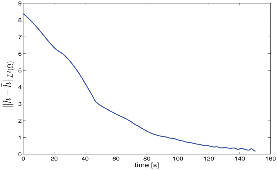
Figure 5 displays the variation of the perturbation energy for the height caused by control law with the following data: $\mathrm{\Omega }=[20,90]\times [0,\frac{\pi }{2}]$ , $\overline{h}=1\mathrm{m}$ , $\overline{u}=\overline{v}=0.02\mathrm{m}/\mathrm{s}$ , and $\mu =5e-05$ with the initial conditions $h^0(x,y)=0.75\mathrm{m}$ and $q^0(x,y)=(0,0)$ using an exponentially decreasing action.

Figure 5.

$L^2$ -norm of the perturbation of the height $h$ in the dimension of time.

The exponential shape of the energy decay showcases the robustness of the control $({\mathcal{V}}_1,{\mathcal{V}}_2)$ . The stabilization rate is chosen very small. Consequently, the decay rate $\exp (-\frac{\mu }{2}{T}_{\phi })$ of the action is close to 1. The action is then decreased sequentially with very small amplitude diminution. It is worth noting that the monotone exponential stability for the 2D nonlinear SWE does not yield from the exponential stability of the linearized SWE. The extension of the approach developed by Coron et al. ²⁵ may produce monotone exponential decay for the nonlinear problem via the linearized problem.

Conclusion

We apply 1D Riemann invariant analysis to build a boundary controller for the 2D shallow water model. In the corresponding 1D stabilization problems, the upstream boundary inflow is chosen as a suitable action on the third characteristic variable. Numerical experiments with a high-resolution dimensionally split finite volume method using Roe linearization shows that the developed control law works on the 2D nonlinear shallow water model, for small stabilization rates. Large stabilization rates give violent flows and the numerical stability issue can be addressed combining continuous and discontinuous Galerkin methods.