A heuristic review on the homotopy perturbation method for non-conservative oscillators

Abstract

The homotopy perturbation method (HPM) was proposed by Ji-Huan. He was a rising star in analytical methods, and all traditional analytical methods had abdicated their crowns. It is straightforward and effective for many nonlinear problems; it deforms a complex problem into a linear system; however, it is still developing quickly. The method is difficult to deal with non-conservative oscillators, though many modifications have appeared. This review article features its last achievement in the nonlinear vibration theory with an emphasis on coupled damping nonlinear oscillators and includes the following categories: (1) Some fallacies in the study of non-conservative issues; (2) non-conservative Duffing oscillator with three expansions; (3)the non-conservative oscillators through the modified homotopy expansion; (4) the HPM for fractional non-conservative oscillators; (5) the homotopy perturbation method for delay non-conservative oscillators; and (6) quasi-exact solution based on He’s frequency formula. Each category is heuristically explained by examples, which can be used as paradigms for other applications. The emphasis of this article is put mainly on Ji-Huan He’s ideas and the present authors’ previous work on the HPM, so the citation might not be exhaustive.

Introduction

Many problems in engineering are essentially nonlinear and are modeled by various nonlinear differential equations. In particular, nonlinear oscillators frequently appear in physics, engineering, biology, and other fields. For example, Fan et al. ¹ found that the low-frequency property of a capillary oscillation plays a vital role in mass and energy transmission in blood flow, permeability, and cell growth. The low frequency is also widely used in energy harvesting devices.^2–4 Additionally, many phenomena can be fully explained by the vibration theory; for example, the release oscillation^5–9 is the main factor affecting the ion release from a hollow fiber, while the thermal oscillation endows a cocoon with a particular bio-function. ¹⁰ The instability of a system also caught much attention to avoid any damage. ¹¹

In general, solving nonlinear differential equations is more complicated than linear differential equations. This paper focuses on a heuristic review on the HPM for non-conservative oscillators by the HPM.^12–13

The HPM has been expansively studied since 1999, and it has matured into a useful mathematics tool thanks to the efforts of many scientists, especially D.D. Ganji, ¹⁴ A. Yildirim, ¹⁵ D. Baleanu, ¹⁶ S. Nadeem, ¹⁷ S.T. Mohyud-din, ¹⁸ Y. Khan, ¹⁹ and others. ²⁰ The convergence of the unprecedented homotopy perturbation method ²¹ was proved by many researchers for various cases,^22–25 and various modifications appeared in the literature. Using the “modified homotopy perturbation method” as a search subject in Clarivate Analytics’ Web of Science, we found more than 400 items. Among all modifications, the He–Laplace method ²⁶ should be specially emphasized. The enhanced homotopy perturbation uses the rank upgrading technique.^27,28 The former was proposed by Xiao-Xia Li and Chun-Hui He and has wide applications^29–31; the latter is a couple of the HPM and the Laplace transform, and it has been proved to be tremendously effective for fractional differential equations.^32–39 The couple of the HPM with other methods has also caught much attention, for example, the generalized differential quadrature method ⁴⁰ and the Fourier transform. ⁴¹ The modifications with an auxiliary term and with two expanding parameters ⁴² are also notable.

During this decade, several works have been accomplished in the development of the oscillation theory by using the HPM. The regular HPM is discussed as follows:

The HPM has overcome the inherent shortcoming of the traditional perturbation method for the small parameter assumption. The homotopy perturbation method is to construct a homotopy equation with an embedding parameter $\rho \in \left[\mathrm{0,1}\right]$ , which is changed from 0 to 1, and used as an expanding parameter for the small parameter in the perturbation method. When $\rho =0$ , the constructed homotopy equation becomes a linear equation, which is easy to be solved, while when $\rho =1$ , it becomes the original one. So the solution process is to deform a linear equation to the nonlinear one gradually, and it converges to the exact solution when $\rho =1$ . As the solution process does not depend on a small parameter in the equation, the solution is uniformly valid for both weakly and strongly nonlinear cases.

Now, to explain the concept of the HPM, we write down an equation in the form

$$L\left(u\right)+N\left(u\right)=f\left(t\right)$$

(1)

where $L$ and N are, respectively, a linear operator and a nonlinear operator, and $f\left(t\right)$ is a known function. A homotopy equation can be constructed as follows

$$H\left(u,\mathrm{\hspace{0.17em}\rho }\right)=\left(1-\rho \right)L\left(u\right)+\rho \left[L\left(u\right)+N\left(u\right)-f\left(t\right)\right]=0,\hspace{1em}\rho \in \left[\mathrm{0,1}\right]$$

or

$$H\left(u,\mathrm{\hspace{0.17em}\rho }\right)=L\left(u\right)+\rho \left(N\left(u\right)-f\left(t\right)\right)=0,\hspace{1em}\rho \in \left[\mathrm{0,1}\right]$$

(2)

where $\rho$ is the homotopy parameter, and it monotonically increases from zero to the unit. The regular HPM is used to search for a solution of equation (2) in a power series in ρ

$$u\left(t,\rho \right)=u_0\left(t\right)+\rho u_1\left(t\right)+{\rho }^2{u}_2\left(t\right)+{\rho }^3{u}_3\left(t\right)+\cdots$$

(3)

Substituting (3) into the family equation (2) which can be rearranged in powers of $\rho$ as

$$H\left(u,\rho \right)=H_0+\rho H_1+{\rho }^2{H}_2+{\rho }^3{H}_3+\cdots =0$$

(4)

where

$$H_0=\underset{\rho \to 0}{\lim }H\left(u,\rho \right)\hspace{0.17em}\text{and}\hspace{0.17em}{H}_n=\frac{1}{n!}\underset{\rho \to 0}{\lim }\frac{{\partial }^{n}H\left(u,\rho \right)}{\partial {\rho }^n}$$

(5)

Due to linearly independence in $\rho$ , the following equations are imposed

$$H_0\left(u_0\right)=0,\hspace{1em}{H}_1\left(u_0,u_1\right)=0,\hspace{1em}{H}_2\left(u_0,u_1,u_2\right)=0,\mathrm{...}$$

(6)

These equations are simpler inhomogeneous linear equations. Solving these equations one by one, we obtain $u_0,u_1,u_2,u_3,\mathrm{...}$ . The approximate solution for equation (1) is found when ρ→1

$$u_{app}\left(t\right)=\underset{\rho \to 1}{\lim }u\left(t,\rho \right)=u_0\left(t\right)+u_1\left(t\right)+u_2\left(t\right)+u_3\left(t\right)+\cdots .$$

(7)

The expansion (3) is suitable for the conservative nonlinear oscillator. The application of the regular HPM to the non-conservative nonlinear oscillator leads to a shortcoming. This shortcoming is surely in the presence of linear damping force as in the case of damping Duffing oscillator where the secular terms due to the perturbations cannot be removed, and the solution cannot be obtained.

In the literature, the frequency is also decomposed into a power series in $\rho$ ,^12–13 but this is not enough for non-conservative oscillators, and the amplitude should also be expressed in a series in $\rho$ . We use the well-known Duffing equation with linear damping as an example to elucidate the idea of three expansions.

Let us consider first the conservative Duffing oscillator

$$\ddot{y}+y+y^3=0,\hspace{1em}y\left(0\right)=A,y^{\prime }\left(0\right)=0$$

(8)

The homotopy function can be built as

$$H\left(y,\rho \right)=\ddot{y}+y+\rho y^3=0,\hspace{1em}\rho \in \left[\mathrm{0,1}\right]$$

(9)

Suppose that the natural frequency and the function $y\left(t;\rho \right)$ have been perturbed in the form

$$1={\omega }^2+\rho {\omega }_1$$

(10)

$$y\left(t,\rho \right)=y_0\left(t\right)+\rho y_1\left(t\right)+{\rho }^2{y}_2\left(t\right)+\cdots .$$

(11)

Substituting (10) and (11) into (9) and setting to zero like power in $\rho$ , we get

$${\rho }^0:{\ddot{y}}_0+{\omega }^2{y}_0=0;\hspace{1em}{y}_0\left(0\right)=A\&{y^{\prime }}_0\left(0\right)=0$$

(12)

$${\rho }^1:{\ddot{y}}_1+{\omega }^2{y}_1=-y_0^3-{\omega }_1{y}_0;\hspace{1em}{y}_1\left(0\right)=0\&{y^{\prime }}_0\left(0\right)=0.$$

(13)

The solution of equation (12) has the form

$$y_0\left(t\right)=A\cos \omega t.$$

(14)

Accordingly, equation (13) becomes

$${\ddot{y}}_1+{\omega }^2{y}_1=-A\left(\frac{3}{4}{A}^2+{\omega }_1\right)\cos \omega t-\frac{A^3}{4}\cos 3\omega t$$

(15)

The secular term can be removed when

$${\omega }_1=-\frac{3}{4}{A}^2$$

(16)

At this end, we have the following approximate solution

$$y\left(t\right)=\left(1-\frac{1}{32{\omega }^2}{A}^2\right)A\cos \left(\omega t\right)+\frac{1}{32{\omega }^2}{A}^3\cos 3\left(\omega t\right)$$

(17)

where $\omega$ is given by

$$\omega =\sqrt{1+\frac{3}{4}{A}^2}$$

(18)

To illustrate that the above procedure cannot succeed for the non-conservative Duffing oscillator, we consider the following damping oscillator

$$\ddot{y}+\mu \dot{y}+y+y^3=0,\hspace{1em}y\left(0\right)=A,y^{\prime }\left(0\right)=0.$$

(19)

According to the above procedure, the homotopy equation corresponding to equation (19) becomes

$$H\left(y,\rho \right)=\ddot{y}+y+\rho \left(\mu \dot{y}+y^3\right)=0,\hspace{1em}\rho \in \left[\mathrm{0,1}\right].$$

(20)

By employing the two expansions (10) and (11) into equation (20) and setting all coefficients of like power of $\rho$ to zero and inserting the zero-order solution (14) into the first-order problems gives

$${\ddot{y}}_1+{\omega }^2{y}_1=-A\left(\frac{3}{4}{A}^2+{\omega }_1\right)\cos \omega t+\mu \omega A\sin \omega t-\frac{A^3}{4}\cos 3\omega t$$

(21)

Since the amplitude $A\ne 0$ , $\mu \ne 0$ , and $\omega \ne 0$ , then there is no reason to eliminate the coefficient of $\sin \omega t$ . According to this shortcoming, we can conclude that the bits of knowledge of the conservative oscillators are not suitable for the non-conservative oscillators.

The homotopy perturbation method always leads to an approximate solution of a nonlinear problem, but sometimes an exact one can be obtained.^43,44 The method was originally proposed to solving differential equations, but it can be used to solve fractal differential equations,^45,46 fractional differential equations, ⁴⁷ and integral equations,^48,49 and difference equations. ⁵⁰ It is extremely effective for inverse problems.^51–53

The strong motive for this work is to avoid errors and erroneous results that occur due to the use of the classical method for problems involving damping forces. Some notes on using the classical homotopy perturbation method for solving the non-conservative oscillators are given in the section Some Fallacies in the Study of Non-Conservative Issues. For a good understanding of the homotopy perturbation method for the non-conservative oscillator, the reader is referred to the section Non-Conservative Duffing Oscillators with Three Expansions, where more developments could be found in the following sections. The basic idea depends on the technology of the normal form used in the damping linear differential equations which leads to derive a total frequency that governs the damping forces besides the restoring forces.

Some fallacies in the study of non-conservative issues

Sometimes, the removal of secular terms can be done, and the solution can be obtained, but these solutions are fakes, and the frequency–amplitude relationship is distorted, is not correct, and does not agree with the numerical solution.

One of the main drawbacks of the classical method is the existence of two different equations that come from avoiding secular terms. These represent two equations covering the same frequency parameter $\Omega$ , and therefore, solutions of these equations will come to different results. The practice is always to try to combine these two equations into one to gain a specific result. It is worth noting that there is no ideal method that can be used in the merging process, which makes the solutions based on frequency accuracy. Therefore, an appropriate amendment must be sought to eliminate such obstacles to obtain the most accurate results. This is the subject of the present issues.

Some may think that using the properties of fractional differentiation may create a situation that can delete the secular terms, and thus, the desired solution can be obtained, but this is an illusion that we will show as follows:

Ex1: The idea is based on applying the fraction homotopy technique by introducing a fraction operator $D^{\alpha +1}$ instead of the operator $D^2$ into equation (19) and then let $\alpha \to 1$ into the final solution. ⁵⁴ Therefore, equation (19) becomes

$$D^{\alpha +1}y+\mu \dot{y}+y+Q{y}^3=0;\hspace{1em}y\left(0\right)=A,\hspace{1em}\dot{y}\left(0\right)=0;\hspace{1em}0<\alpha \le 1$$

(22)

The operator refers to the time-fractional operator obeys the definition of the Riemann–Liouville time-fractional derivative.

The corresponding homotopy equation becomes

$$D^{2}y+y+\rho \left(D^{\alpha +1}y+\mu \dot{y}-D^{2}y+Q{y}^3\right)=0;\hspace{1em}\rho \in \left[\mathrm{0,1}\right]$$

(23)

By inserting the two expansions (10) and (11) into (23), for setting the identical power of $\rho$ to zero, yields

$${\ddot{y}}_1+{\omega }^2{y}_1={\omega }_1{y}_0-\left(D^{\alpha +1}{y}_0+\mu {\dot{y}}_0-{\ddot{y}}_0+Q{y}_0^3\right)$$

(24)

Employing the zero-order solution (14) into (24) and using the appendix yields

$${\ddot{y}}_1+{\omega }^2{y}_1=-A\cos \omega t\left({\omega }_1+{\omega }^2+\frac{3}{4}{A}^{2}Q-{\omega }^{\alpha +1}\sin \left(\frac{1}{2}\pi \alpha \right)\right)+A\sin \omega t\left(-\mu \omega -{\omega }^{\alpha +1}\cos \left(\frac{1}{2}\pi \alpha \right)\right)-\frac{1}{4}{A}^{3}Q\cos 3\omega t$$

(25)

Dropping the secular terms from (25) requires

$${\omega }_1=-{\omega }^2-\frac{3}{4}{A}^{2}Q+{\omega }^{\alpha +1}\sin \left(\frac{1}{2}\pi \alpha \right)$$

(26)

$$\mu \omega =-{\omega }^{\alpha +1}\cos \left(\frac{1}{2}\pi \alpha \right)$$

(27)

Then the total solution of (25) without secular terms is

$$y_1\left(t\right)=\frac{A^{3}Q}{32{\omega }^2}\left(\cos 3\omega t-\cos \omega t\right)$$

(28)

To construct the frequency–amplitude relationship, we may combine (26) and (27) through the elimination ${\omega }^{\alpha +1}$ between them and inserting the result into the expansion (10) and letting $\rho \to 1$ yields

$$\left(1+\frac{3}{4}{A}^{2}Q\right)\cos \left(\frac{1}{2}\pi \alpha \right)+\mu \omega \sin \left(\frac{1}{2}\pi \alpha \right)=0.$$

(29)

Setting $\alpha \to 1$ into the above relation leads to $\mu \omega =0$ . In other words, inserting (26) into expansion (10) and setting $\rho \to 1$ becomes

$$1+\frac{3}{4}{A}^{2}Q={\omega }^{\alpha +1}\sin \left(\frac{1}{2}\pi \alpha \right)$$

(30)

Square (30) and adding to the squaring of (27) and setting $\alpha =1$ result into the following relation

$${\omega }^4-{\mu }^2{\omega }^2-{\left(1+\frac{3}{4}{A}^{2}Q\right)}^2=0$$

(31)

Since for periodic solution, the above relation must have positive roots, which cannot occur because the last term is always negative. Finally, they overcome the difficulty though the fraction calculus fails.

Ex2: Given the Rayleigh oscillator in the form ⁵⁵

$$\ddot{y}+a_1\dot{y}+a_{0}y+a_{2}y{\dot{y}}^2+a_3{\dot{y}}^3=0;\hspace{1em}y\left(0\right)=A,\hspace{1em}\dot{y}\left(0\right)=0$$

(32)

where $a_j;\hspace{0.17em}j=0:3$ are known real constants.

Construct the homotopy equation in the form

$$\ddot{y}+a_{0}y+\rho \left(a_1\dot{y}+a_{2}y{\dot{y}}^2+a_3{\dot{y}}^3\right)=0;\hspace{1em}\rho \in \left[\mathrm{0,1}\right].$$

(33)

Considering the frequency analysis so that we define the following frequency expansion

$${\Omega }^2=a_0+\rho {\Omega }_1+{\rho }^2{\Omega }_2+\cdots .$$

(34)

Employing (34) and (11) with (33), equating the identical powers of $\rho$ to zero yields the zero-order solution

$$y_0\left(t\right)=A\cos \Omega t$$

(35)

The first-order problem has the form

$${\ddot{y}}_1+{\Omega }^2{y}_1={\Omega }_1{y}_0-a_2{\dot{y}}_0^2{y}_0-a_1{\dot{y}}_0-a_3{\dot{y}}_0^3,y_1\left(0\right)=0,{\dot{y}}_1\left(0\right)=0$$

(36)

Substituting (35) into (36), the requirement of no secular term in $y_1\left(t\right)$ needs

$${\Omega }_1=\frac{1}{4}{A}^2{\Omega }^2{a}_2\hspace{1em}\text{and}$$

(37)

$${\Omega }^2=-\frac{4a_1}{3a_3{A}^2}$$

(38)

Solution of (36) without secular terms yields

$$y_1\left(t\right)=-\frac{A^3{a}_2}{32}\left(\cos 3\Omega t-\cos \Omega t\right)+\frac{A^3\Omega a_3}{32}\left(\sin 3\Omega t-3\sin \Omega t\right)$$

(39)

We, therefore, obtain

$$y\left(t\right)=A\cos \Omega t-\frac{A^3{a}_2}{32}\left(\cos 3\Omega t-\cos \Omega t\right)+\frac{A^3\Omega a_3}{32}\left(\sin 3\Omega t-3\sin \Omega t\right)$$

(40)

To find the frequency–amplitude relationship, from equation (34) by setting $\rho \to 1$ , we have

$${\Omega }^2=\frac{a_0}{1-\left(1/4\right)A^2{a}_2}$$

(41)

Another frequency equation is given by (38). Then there is duplication for the frequency–amplitude relationship. This represents a shortcoming in applying the regular homotopy perturbation method. The following examples can illustrate some of this fallacy:

Ex3: Consider the following delay harmonic second-order equation ⁵⁶

$$\ddot{y}+\mu \dot{y}+\sigma y\left(t-\tau \right)=0;\hspace{1em}y\left(0\right)=A,\dot{y}\left(0\right)=0$$

(42)

where $\mu \text{ and }\sigma$ are constant coefficients and $\tau$ refers to the time delay. If $\tau \to 0$ , the coefficient $\sigma$ will play as natural frequency. For nonzero $\tau$ , this equation leads to obtaining non-oscillation solutions. In order to obtain an oscillation solution, we need to modify it by introducing the missing term in an artificial way. Rewrite equation (42) in an equivalent type

$$\ddot{y}+\mu \dot{y}+{\Omega }^{2}y+\sigma y\left(t-\tau \right)-{\Omega }^{2}y=0;\hspace{1em}y\left(0\right)=A,\dot{y}\left(0\right)=0$$

(43)

To obtain a periodic solution, the frequency $\Omega$ must be chosen to have real and positive values.

At this stage, we can choose the two parts as

$$L\left(y\right)=\ddot{y}+{\Omega }^{2}y,\hspace{0.17em}\text{and}\hspace{0.17em}N\left(y\right)=\mu \dot{y}+\sigma y\left(t-\tau \right)-{\Omega }^{2}y$$

(44)

Construct the following homotopy equation

$$\begin{array}{l}H\left(y,\rho \right)=L\left(y\right)+\rho N\left(y\right)=0\\ =\left(\ddot{y}+{\Omega }^{2}y\right)+\rho \left(\mu \dot{y}+\sigma y\left(t-\tau \right)-{\Omega }^{2}y\right)=0;\hspace{1em}\rho \in \left[\mathrm{0,1}\right]\end{array}$$

(45)

Substituting the regular expansion (11) into (45), we obtain the following linear system

$${\ddot{y}}_0+{\Omega }^2{y}_0=0,\hspace{1em}{y}_0\left(0\right)=A,\hspace{1em}{\dot{y}}_0\left(0\right)=0$$

(46)

$${\ddot{y}}_1+{\Omega }^2{y}_1={\Omega }^2{y}_0-\mu {\dot{y}}_0-\sigma y_0\left(t-\tau \right),\hspace{1em}{y}_1\left(0\right)=0,\hspace{1em}{\dot{y}}_1\left(0\right)=0$$

(47)

The solution of equation (46) is equation (35). Consequently, we have

$$y_0\left(t-\tau \right)=A\cos \Omega \left(t-\tau \right)=A\cos \Omega t\cos \Omega \tau +A\sin \Omega t\sin \Omega \tau$$

(48)

Substituting (35) and (48) into equation (47) yields

$${\ddot{y}}_1+{\Omega }^2{y}_1=A\left({\Omega }^2-\sigma \cos \Omega \tau \right)\cos \Omega t+A\left(\mu \Omega -\sigma \sin \Omega \tau \right)\sin \Omega t$$

(49)

For the bounded solution, we must eliminate terms that produce secular terms from equation (49)

$$\sigma \cos \Omega \tau ={\Omega }^2\hspace{0.17em}\text{and}\hspace{0.17em}\sigma \sin \Omega \tau =\mu \Omega$$

(50)

The absence of the parameter $\tau$ will lead to a shortcoming. Therefore, the presence of $\tau$ is important to avoid the shortcoming. To find the frequency equation, from equation (50) and by a simple calculation, we have

$${\Omega }^4+{\mu }^2{\Omega }^2-{\sigma }^2=0$$

(51)

It is noted that the impact of the time delay $\tau$ is absent in the frequency equation (51) and so will be absent in the final solution. Accordingly, there is an allowance to discuss the implications of $\tau$ in the solution. However, by dropping the secular terms, the solution of the first-order problem because of the initial conditions becomes $y_1\left(t\right)=0$ . At this stage, the complete solution for the homotopy equation (45) is given as

$$y\left(t\right)=A\cos \Omega t$$

(52)

To ensure that there is a periodic solution, the frequency $\Omega$ governed by the frequency equation (51) must be real. But equation (51) is a quadratic in ${\Omega }^2$ . Since the middle term is fully positive and the last term is full negative, then there are no two alternative signs. Therefore, ${\Omega }^2$ cannot be positive. Consequently, the periodic solution cannot be found. At this stage, the frequency equation and the solution (13) are fakes.

Since equation (42) is a second-order linear equation, then its exact solution can be formulated in the case of a small time-delay parameter $\tau$ . In neglecting ${\tau }^2$ in the Taylor expansion, the function $y\left(t-\tau \right)$ can be expanded as

$$y\left(t-\tau \right)=y\left(t\right)-\tau \dot{y}\left(t\right)$$

(53)

Inserting equation (53) into the original equation (42) becomes

$$\ddot{y}\left(t\right)+\left(\mu -\tau \sigma \right)\dot{y}\left(t\right)+\sigma y\left(t\right)=0$$

(54)

Its exact solution through the normal form technique results in the form

$$y\left(t\right)=A{e}^{\left(1/2\right)\left(\tau \sigma -\mu \right)t}\cos t\sqrt{\sigma -\frac{1}{4}{\left(\mu -\tau \sigma \right)}^2}$$

(55)

Ex4: Consider the following delay Duffing equation ⁵⁷

$$\ddot{y}+\mu \dot{y}+\sigma y\left(t-\tau \right)+\beta y^3;\hspace{1em}y\left(0\right)=A,\dot{y}\left(0\right)=0$$

(56)

One can think that the presence of the term delayed can suppress the weakness of the damped Duffing equation. Again, we will show that this belief is not true.

Convert equation (56) into the following equivalent type

$$\ddot{y}+\mu \dot{y}+{\Omega }^{2}y+\sigma y(t-\tau )-{\Omega }^{2}y+\beta y^3;\hspace{0.17em}\hspace{0.17em}\hspace{0.17em}\hspace{0.17em}\hspace{0.17em}\hspace{0.17em}\hspace{0.17em}\hspace{0.17em}\hspace{0.17em}y\left(0\right)=A,\hspace{0.17em}\hspace{0.17em}\dot{y}\left(0\right)=0.$$

(57)

Construct the following homotopy equation

$$\left(\ddot{y}+{\Omega }^{2}y\right)+\rho \left(\mu \dot{y}+\sigma y\left(t-\tau \right)-{\Omega }^{2}y+\beta y^3\right)=0;\hspace{1em}\rho \in \left[\mathrm{0,1}\right]$$

(58)

Substituting the regular expansion (11) in the previous example into the above equation and rearranged in terms of powers of $\rho$ , we obtain the following equations

$${\ddot{y}}_0+{\Omega }^2{y}_0=0,\hspace{1em}{y}_0\left(0\right)=A,\hspace{1em}{\dot{y}}_0\left(0\right)=0$$

(59)

$${\ddot{y}}_1+{\Omega }^2{y}_1={\Omega }^2{y}_0-\mu {\dot{y}}_0-\sigma y_0\left(t-\tau \right)-\beta y_0^3,\hspace{1em}{y}_1\left(0\right)=0,\hspace{1em}{\dot{y}}_1\left(0\right)=0.$$

(60)

Substituting (35) and (48) into the first-order problem (60) yields

$$\begin{array}{l}{\ddot{y}}_1+{\Omega }^2{y}_1={\Omega }^{2}A\cos \Omega t+\mu \Omega A\sin \Omega t-\sigma A\cos \Omega t\cos \Omega \tau -\sigma A\sin \Omega t\sin \Omega \tau -\beta A^3{\cos }^3\Omega t\\ =A\left({\Omega }^2-\frac{3}{4}\beta A^2-\sigma \cos \Omega \tau \right)\cos \Omega t+A\left(\mu \Omega -\sigma \sin \Omega \tau \right)\sin \Omega t-\frac{1}{4}\beta A^3\cos 3\Omega t\end{array}$$

(61)

For a uniform solution, we must eliminate terms that produce secular terms from equation (61) to become

$${\ddot{y}}_1+{\Omega }^2{y}_1=-\frac{1}{4}\beta A^3\cos 3\Omega t$$

(62)

with the following solvability conditions

$$\sigma \cos \Omega \tau ={\Omega }^2-\frac{3}{4}\beta A^2\hspace{0.17em}\text{and}\hspace{0.17em}\sigma \sin \Omega \tau =\mu \Omega$$

(63)

Squaring and adding to formulate the following frequency equation

$${\Omega }^4-\left(\frac{3}{2}\beta A^2-{\mu }^2\right){\Omega }^2+\left(\frac{9}{16}{\beta }^2{A}^4-{\sigma }^2\right)=0$$

(64)

Now, we have the following condition that must ensure that ${\Omega }^2$ is positive

$$\frac{3}{2}\beta A^2>{\mu }^2\&\frac{9}{16}{\beta }^2{A}^4>{\sigma }^2$$

(65)

It remains another condition that is the discriminant must be positive to gain real roots of (64). It is easy to show that the discriminant $\Delta ={\left(\frac{3}{2}\beta A^2-{\mu }^2\right)}^2+4{\sigma }^2-\frac{9}{4}{\beta }^2{A}^4$ cannot be positive. This discriminant can be arranged as a polynomial quadratic in $\mu$ , that is, $\left({\mu }^4-3\beta A^2{\mu }^2+4{\sigma }^2\right)$ . This polynomial will be positive if for all, $\mu$ and its discriminant must be negative. This aim requires

$$9{\beta }^2{A}^4<16{\sigma }^2$$

(66)

Satisfying conditions (66) should ensure that the roots of equation (64) are real. But this condition conflicts with the last condition in (65). So the frequency equation (64) is improper. Further, any solution that depends on (64) fakes.

According to failures found in the above examples, it is urgent to search for another technique to treat the nonlinear damping oscillators.

Non-conservative Duffing oscillators with three expansions

This section considers the damped Duffing equation, which has wide applications in engineering.

Ex5: The non-conservative Duffing equation is given as follows

$$\ddot{y}+\mu \dot{y}+{\omega }_0^{2}y+Q{y}^3=0;\hspace{1em}y=y\left(t\right)$$

(67)

This equation is difficult to be solved by the traditional homotopy perturbation method, and here is used a modification suggested by He and El-Dib in Ref. [58], where the solution, frequency, and amplitude are expanded in series of ρ.

The homotopy equation corresponding to equation (67) is

$$\ddot{y}+{\omega }_0^{2}y=-\rho \left(\mu \dot{y}+Q{y}^3\right);\hspace{1em}\rho \in \left[\mathrm{0,1}\right]$$

(68)

By a similar operation as above, we have the zero-order linear equation

$${\ddot{y}}_0+{\omega }_0^2{y}_0=0$$

(69)

Its exact solution is

$$y_0\left(t\right)=A_0\cos \left({\omega }_{0}t+\theta \right)$$

(70)

where $A_0$ and $\theta$ are identified by the initial conditions.

Only one expansion is not enough, and for nonlinear oscillator, we also use the following expansion^12–13

$${\omega }_0^2\left(\rho \right)={\omega }^2-\rho {\omega }_1-{\rho }^2{\omega }_2+\cdots$$

(71)

where $\omega$ is the frequency to be further determined; and ${\omega }_j$ are identified in view of no security term in $y_j$ .

The two expansions given in equation (11) and (71) are effective for the conservative case, and for non-conservative oscillators, the amplitude $A$ has to be expanded in the form

$$A\left(t,\rho \right)=\alpha \left(1+\rho C_1\left(t\right)+{\rho }^2{C}_2\left(t\right)+\cdots \right)$$

(72)

where the unknowns $C_j\left(t\right)$ can be determined as the same rule for the determination of ${\omega }_j$ . In view of equations (71) and (72), equation (70) becomes

$$y_0(t;\rho )=\alpha (1+\rho C_1\left(t\right)+{\rho }^2{C}_2\left(t\right)+\mathrm{...})\cos \left(\omega t+\theta \right)\hspace{0.17em}.$$

(73)

When $\rho \to 0$ , we have $A\to A_0$ and $\omega \to {\omega }_0.$ Consequently, expansion (73) will convert to the solution (70). Thus, we have

$$y_0\left(t;0\right)=A_0\cos \left({\omega }_{0}t+\theta \right)$$

(74)

$$y_0\left(t;1\right)=\alpha \left(1+C_1\left(t\right)+C_2\left(t\right)+\cdots \right)\cos \left(\omega t+\theta \right)$$

(75)

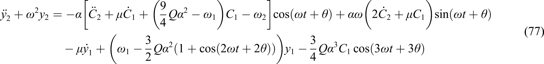
In view of equations (11), (71), and (73), from equation (68), we can obtain the following linear system

$${\ddot{y}}_1+{\omega }^2{y}_1=-\alpha \left({\ddot{C}}_1+\frac{3}{4}Q{\alpha }^2-{\omega }_1\right)\cos \left(\omega t+\theta \right)+\alpha \omega \left(\mu +2{\dot{C}}_1\right)\sin \left(\omega t+\theta \right)-\frac{1}{4}Q{\alpha }^3\cos \left(3\omega t+3\theta \right)$$

(76)

$$\begin{array}{l}{\ddot{y}}_2+{\omega }^2{y}_2=-\alpha \left[{\ddot{C}}_2+\mu {\dot{C}}_1+\left(\frac{9}{4}Q{\alpha }^2-{\omega }_1\right)C_1-{\omega }_2\right]\cos \left(\omega t+\theta \right)+\alpha \omega \left(2{\dot{C}}_2+\mu C_1\right)\sin \left(\omega t+\theta \right)\\ -\mu {\dot{y}}_1+\left({\omega }_1-\frac{3}{2}Q{\alpha }^2\left(1+\cos \left(2\omega t+2\theta \right)\right)\right)y_1-\frac{3}{4}Q{\alpha }^3{C}_1\cos \left(3\omega t+3\theta \right)\end{array}$$

(77)

To guarantee a periodic solution, the coefficients of $\cos \left(\omega t+\theta \right)$ and $\sin \left(\omega t+\theta \right)$ in equation (76) must be zero

$${\ddot{C}}_1={\omega }_1-\frac{3}{4}Q{\alpha }^2\&$$

(78)

$${\dot{C}}_1=-\frac{1}{2}\mu$$

(79)

The solution of equation (76) reads

$$y_1\left(t\right)=\frac{Q{\alpha }^3}{32{\omega }^2}\cos \left(3\omega t+3\theta \right)$$

(80)

Similarly, the periodic solution for equation (77) requires

$${\omega }_2={\ddot{C}}_2+\mu {\dot{C}}_1+\left(\frac{9}{4}Q{\alpha }^2-{\omega }_1\right)C_1+\frac{3Q^2{\alpha }^4}{128{\omega }^2}$$

(81)

$${\dot{C}}_2=-\frac{1}{2}\mu C_1$$

(82)

Using the above results, we obtain

$$\begin{array}{l}{y}_2\left(t\right)=\frac{Q{\alpha }^3}{256{\omega }^4}\left(-{\omega }_1+\frac{3Q{\alpha }^2}{2}\right)\cos \left(3\omega t+3\theta \right)-\frac{3\mu Q{\alpha }^3}{256{\omega }^3}\sin \left(3\omega t+3\theta \right)+\frac{3Q^2{\alpha }^5}{3072{\omega }^4}\cos \left(5\omega t+5\theta \right)\\ -\frac{3Q{\alpha }^3}{4\left(D^2+{\omega }^2\right)}{C}_1\left(t\right)\cos \left(3\omega t+3\theta \right)\end{array}$$

(83)

Solving $C_1$ from equation (79) yields

$$C_1\left(t\right)=-\frac{1}{2}\mu t$$

(84)

From equation (82), $C_2$ can be solved as

$$C_2\left(t\right)=\frac{1}{8}{\mu }^2{t}^2$$

(85)

In view of equations (78) and (79), we can solve ${\omega }_1$ from equation (78), which is

$${\omega }_1=\frac{3Q{\alpha }^2}{4}$$

(86)

Similarly, from equation (81), we have

$${\omega }_2=-\frac{1}{4}{\mu }^2-\frac{3}{4}Q{\alpha }^2\mu t+\frac{3Q^2{\alpha }^4}{128{\omega }^2}$$

(87)

Finally, from equation (71), we obtain

$${\omega }^2={\omega }_0^2-\frac{1}{4}{\mu }^2+\frac{3Q{\alpha }^2}{4}\left(1-\mu t+\cdots \right)+\frac{3Q^2{\alpha }^4}{128{\omega }^2}$$

(88)

Considering $e^{-\mu t}=1-\mu t+\cdots$ , we write equation (88) in the form

$${\omega }^2={\omega }_0^2-\frac{1}{4}{\mu }^2+\frac{3Q{\alpha }^2}{4}{e}^{-\mu t}+\frac{3Q^2{\alpha }^4}{128{\omega }^2}$$

(89)

This frequency formulation shows the damping effect on the frequency. When $\mu \to 0$ , equation (89) turns out to be the classical frequency formulation.

Further, in view of equations (84) and (85), from equation (72), we have

$$A\left(t\right)=\alpha \left[1-\left(\frac{1}{2}\mu t\right)+\frac{1}{2}{\left(\frac{1}{2}\mu t\right)}^2+\cdots \right]$$

(90)

Equation (90) can be expressed in the form

$$A\left(t\right)=\alpha e^{-\left(1/2\right)\mu t}$$

(91)

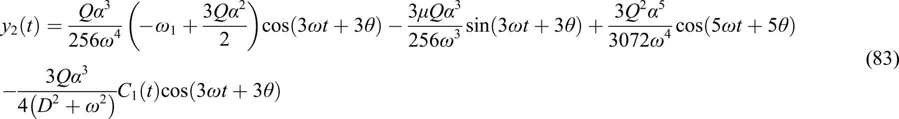
In view of equation (91), our result given in equation (73) leads to that for the linear harmonic equation when the nonlinear term is ignored.

In view of equations (91), (80), and (84), we obtain the following second-order approximate solution from equation (77)

$$y\left(t\right)=\alpha e^{-\left(1/2\right)\mu t}\cos \left(\omega t+\theta \right)+\frac{Q{\alpha }^3}{32{\omega }^2}\left(e^{-\left(3/2\right)\mu t}+\frac{3Q{\alpha }^2}{32{\omega }^3}\right)\cos \left(3\omega t+3\theta \right)+\frac{3\mu Q{\alpha }^3}{128{\omega }^3}\sin \left(3\omega t+3\theta \right)+\frac{3Q^2{\alpha }^5}{3072{\omega }^4}\cos \left(5\omega t+5\theta \right)$$

(92)

This solution is consistent with the solution when $\mu \to 0$ by the standard homotopy perturbation method.

It should be pointed out that μ > 0 for practical applications, and the frequency must be positive. To study its stability criteria, we rewrite equation (89) by introducing an artificial parameter ε

$${\omega }^2={\omega }_0^2-\frac{1}{4}{\mu }^2+\epsilon \left(\frac{3Q{\alpha }^2}{4}{e}^{-\epsilon \mu t}+\frac{3Q^2{\alpha }^4}{128{\omega }^2}\right);\hspace{1em}\epsilon \in \left[\mathrm{0,1}\right]$$

(93)

Using the traditional perturbation method to expand ω

$${\omega }^2={\Omega }_0^2+\epsilon {\Omega }_1+{\epsilon }^2{\Omega }_2+\cdots$$

(94)

By a simple operation as required by the perturbation method, we obtain

$${\Omega }_0=\sqrt{{\omega }_0^2-\frac{1}{4}{\mu }^2}$$

(95)

$${\Omega }_1=\frac{3Q{\alpha }^2}{4}+\frac{3Q^2{\alpha }^4}{128\left({\omega }_0^2-\left(1/4\right){\mu }^2\right)}$$

(96)

By setting $\epsilon =1$ in equation (94), we obtain

$${\omega }^2={\omega }_0^2-\frac{1}{4}{\mu }^2+\frac{3}{4}Q{\alpha }^2+\frac{3Q^2{\alpha }^4}{128\left({\omega }_0^2-\left(1/4\right){\mu }^2\right)}$$

(97)

The stability conditions are

$$\mu >0,\hspace{0.17em}\text{and}\hspace{0.17em}{\omega }_0^2-\frac{1}{4}{\mu }^2+\frac{3}{4}Q{\alpha }^2+\frac{3Q^2{\alpha }^4}{128\left({\omega }_0^2-\left(1/4\right){\mu }^2\right)}>0$$

(98)

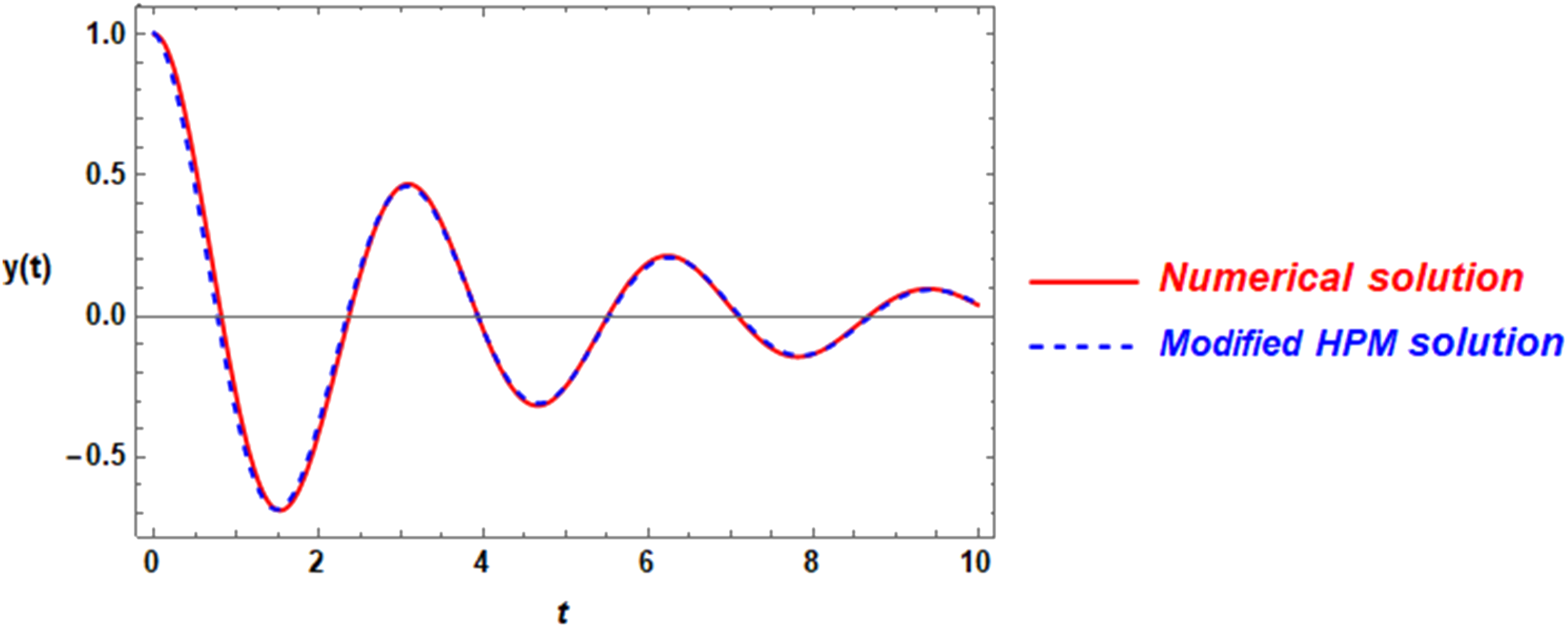
When $\mu =0$ , the stability conditions are the same as those obtained by the traditional homotopy perturbation method.^12–13 The comparison of our result with the numerical one is given in Figure 1 for some given parameters, and a good agreement is found.

Figure 1.

Comparison of the approximate solution of equation (92) with the numerical one when ${\omega }_0=2,\mu =0.5,Q=0.5,\theta =0,\text{ and }\alpha =1$ .

Ex6: The equations describing the lateral vibrations of a horizontally supported Jeffcott rotor system are given as follows ⁵⁹

$$\begin{array}{l}\ddot{x}+{\mu }_1\dot{x}+{\omega }_1^{2}x+Q_1{x}^3=\delta x{y}^2\\ \ddot{y}+{\mu }_2\dot{y}+{\omega }_2^{2}y+Q_2{y}^3=\delta y{x}^2\end{array}$$

(99)

where ${\mu }_i$ represents the damping coefficient, $Q_i$ refers to the Duffing coefficient, $\delta$ measures the strength of the interaction, and ${\omega }_i$ denotes the linear frequency. The above system is subject to the initial conditions: $x\left(0\right)=A,\stackrel{\hspace{0.17em}\dot{}}{x}\left(0\right)=0,\mathrm{\hspace{0.17em}y}\left(0\right)=\hspace{0.17em}B\&\hspace{0.17em}\dot{y}\left(0\right)=0$ . The above system represents a good application to the Duffing oscillator with three expansions given in the last example.

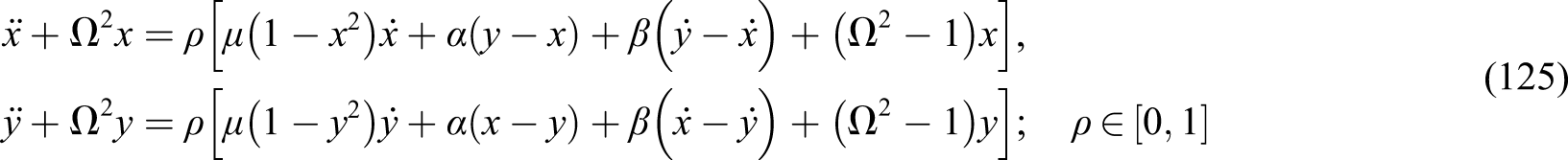
Suppose that the above system has a common frequency $\Omega$ . By introducing this frequency into the system (99) becomes

$$\begin{array}{l}\ddot{x}+{\Omega }^{2}x=\delta x{y}^2-{\mu }_1\dot{x}+\left({\Omega }^2-{\omega }_1^2\right)x-Q_1{x}^3,\\ \ddot{y}+{\Omega }^{2}y=\delta y{x}^2-{\mu }_2\dot{y}+\left({\Omega }^2-{\omega }_2^2\right)y-Q_2{y}^3\end{array}$$

(100)

Establish the corresponding homotopy equations in the form

$$\begin{array}{l}\ddot{x}+{\Omega }^{2}x=\rho \left(\delta x{y}^2-{\mu }_1\dot{x}+\left({\Omega }^2-{\omega }_1^2\right)x-Q_1{x}^3\right),\\ \ddot{y}+{\Omega }^{2}y=\rho \left(\delta y{x}^2-{\mu }_2\dot{y}+\left({\Omega }^2-{\omega }_2^2\right)y-Q_2{y}^3\right);\hspace{1em}\rho \in \left[\mathrm{0,1}\right]\end{array}$$

(101)

Supposing the suggested solutions can be expanded in the form

$$\begin{array}{l}x\left(t;\rho \right)=e^{-\frac{1}{2}\hspace{0.17em}\rho {\mu }_{1}t}\left(x_0\left(t\right)+\rho x_1\left(t\right)+{\rho }^2{x}_2\left(t\right)+\cdots \right),\\ y\left(t;\rho \right)=e^{-\frac{1}{2}\hspace{0.17em}\rho {\mu }_{2}t}\left(y_0\left(t\right)+\rho y_1\left(t\right)+{\rho }^2{y}_2\left(t\right)+\cdots \right)\end{array}$$

(102)

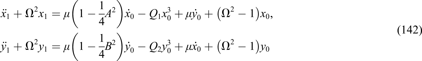
Substituting (102) into (101) and equating like powers of $\rho$ to zero, yields

$$x_0\left(t\right)=A\cos \Omega t\&y_0\left(t\right)=B\cos \Omega t$$

(103)

The first-order problem is given by

$$\begin{array}{l}{\ddot{x}}_1+{\Omega }^2{x}_1=\delta x{y}_0^2-{\mu }_1{\dot{x}}_0+\left({\Omega }^2-{\omega }_1^2\right)x_0-Q_1{x}_0^3,\\ {\ddot{y}}_1+{\Omega }^2{y}_1=\delta y{x}_0^2-{\mu }_2{\dot{y}}_0+\left({\Omega }^2-{\omega }_2^2\right)y_0-Q_2{y}_0^3\end{array}$$

(104)

Insert (103) into (104) and dropping the secular terms gives

$$\begin{array}{l}{\Omega }^2-{\omega }_1^2-\frac{3}{4}{Q}_1{A}^2+\frac{3}{4}\delta B^2=0,\\ {\Omega }^2-{\omega }_2^2-\frac{3}{4}{Q}_2{B}^2+\frac{3}{4}\delta A^2=0\end{array}$$

(105)

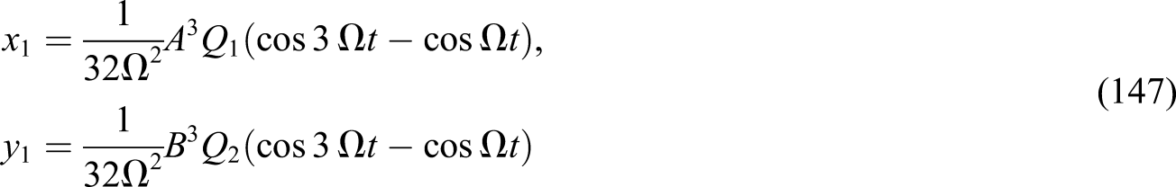
Under these solvability conditions (105), the solutions of the system (104) become

$$\begin{array}{l}{x}_1\left(t\right)=\frac{A}{32{\Omega }^2}\left(A^2{Q}_1-B^2\delta \right)\left(\cos 3\Omega t-\cos \Omega t\right),\\ y_1\left(t\right)=\frac{B}{32{\Omega }^2}\left(B^2{Q}_2-A^2\delta \right)\left(\cos 3\Omega t-\cos \Omega t\right).\end{array}$$

(106)

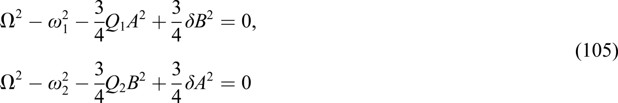
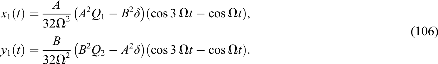
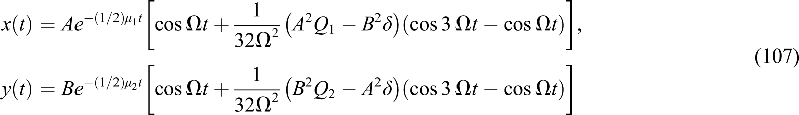
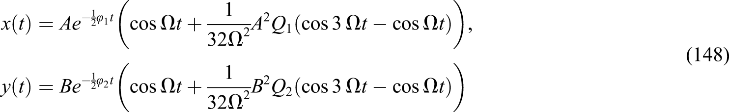
Employing (103) and (106) into the expansions (102) and letting $\rho \to 1$ yield the first-order approximate solutions in the form

$$\begin{array}{l}x\left(t\right)=A{e}^{-\left(1/2\right){\mu }_{1}t}\left[\cos \Omega t+\frac{1}{32{\Omega }^2}\left(A^2{Q}_1-B^2\delta \right)\left(\cos 3\Omega t-\cos \Omega t\right)\right],\\ y\left(t\right)=B{e}^{-\left(1/2\right){\mu }_{2}t}\left[\cos \Omega t+\frac{1}{32{\Omega }^2}\left(B^2{Q}_2-A^2\delta \right)\left(\cos 3\Omega t-\cos \Omega t\right)\right]\end{array}$$

(107)

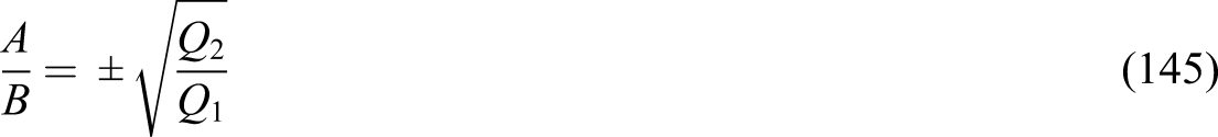
To establish the frequency–amplitude equation, we need to combine the solvability conditions that are given in (105). This aim may require to multiply the first equation of (105) by ${\omega }_2^2$ and subtracted from the second equation multiplied by ${\omega }_1^2$ yields

$${\Omega }^2=\frac{3}{4\left({\omega }_2^2-{\omega }_1^2\right)}\left[\left(Q_1{A}^2-\delta B^2\right){\omega }_2^2-\left(Q_2{B}^2-\delta A^2\right){\omega }_1^2\right]$$

(108)

At this stage, we may distinguish between two cases concerned to the relation of ${\omega }_1^2$ and ${\omega }_2^2$ . The first case where ${\omega }_2^2\ne {\omega }_1^2$ is known as the non-resonance case. The second case deals with the approaching of ${\omega }_2^2$ to ${\omega }_1^2$ . The last case is known as the internal resonance case.

For the internal resonance case, we may express the nearness of ${\omega }_2^2$ to ${\omega }_1^2$ by introducing a parameter $\sigma$ defining as

$${\omega }_2^2={\omega }_1^2+\sigma$$

(109)

Employing (109) with (105), one can estimate $\sigma$ to be

$$\sigma =\frac{3}{4}\left[\left(Q_1+\delta \right)A^2-\left(Q_2+\delta \right)B^2\right]$$

(110)

At this end, the frequency $\Omega$ becomes

$${\Omega }^2={\omega }_1^2+\frac{3}{4}\left(Q_1{A}^2-\delta B^2\right)$$

(111)

The non-conservative oscillators through the modified homotopy expansion

To avoid the fails in solving the damping oscillators, EL-Dib^60,61 uses the following modification for the homotopy exposition

$$y\left(t;\rho \right)=e^{-\left(1/2\right)\rho \phi t}\left(y_0\left(t\right)+\rho y_1\left(t\right)+{\rho }^2{y}_2\left(t\right)+\cdots \right)$$

(112)

The damping term $\left(e^{-\left(1/2\right)\rho \phi t}\right)$ is important for a damped oscillation. When $\phi \to 0$ , equation (112) reduces to the original one required by the homotopy perturbation method. It is noted that the parameter $\phi$ refers to all linear and nonlinear coefficients given in the nonlinear oscillators. It will be $\mu$ the damping coefficient of the simple damping Duffing oscillator. In the above examples Ex2 and Ex3, we can summarize the suitable decay parameter $\phi$ in each example. In Ex1, the suitable $\phi =\mu \omega +{\omega }^{\alpha +1}\cos \left(\left(1/2\right)\pi \alpha \right)$ , and in Ex2, the damping parameter $\phi$ is constructed from the linear damping coefficient $a_1$ and the cubic nonlinear damping coefficient $a_3$ to be $\phi =a_1+\left(3/4\right)a_3{A}^2{\Omega }^2$ , and in Ex3 and Ex4, the damping parameter becomes φ = μ − (σ/Ω)sinΩτ.

The question now is how the damping parameter $\phi$ can be estimated. Usually, in the homotopy perturbations for the conservative oscillations, there is only one solvability condition used to determine the frequency–amplitude relationship. The application of the homotopy perturbation technique through the modified homotopy expansion will impose two solvability conditions: one of them used to construct the frequency equation and the second one used to determine the parameter $\phi$ . The absence of the parameter $\phi$ in the analysis of the non-conservative oscillator will lead to producing two solvability conditions in terms of the frequency parameter, and so duplication in the frequency equations occurs, which will produce wrong solutions.

In what follows, some examples are derived from the illustration:

Ex7: Consider the following Van der Pol oscillator ⁶²

$$\ddot{y}-\mu \left(1-y^2\right)\dot{y}+y=0,\hspace{1em}y\left(0\right)=A,\dot{y}\left(0\right)=0$$

(113)

where $\mu >0$ is the coefficient of the damping force.

To solve equation (113), we first write the corresponding homotopy equation in the form

$$\ddot{y}+y=\rho \mu \left(1-y^2\right)\dot{y};\hspace{1em}\rho \in \left[\mathrm{0,1}\right]$$

(114)

where the unknowns $\phi$ and $y_n\left(t\right)$ will be determined later. Inserting (112) into (114) and then setting the coefficient of the identical powers $\rho$ to zero yields the zero-order solution in the form

$$y_0\left(t\right)=A\cos t$$

(115)

The first-order problem is

$${\ddot{y}}_1+y_1=\phi {\dot{y}}_0+\mu \left(1-y_0^2\right){\dot{y}}_0$$

(116)

Employing (115) with (116) and dropping the secular terms yields

$$\phi =-\mu \left(1-\frac{1}{4}{A}^2\right)$$

(117)

Free of the secular terms equation (116) has the solution

$$y_1=-\frac{1}{32}\mu A^3\left(\sin 3t-3\sin t\right)$$

(118)

The first-order solution can be formulated in the form

$$y\left(t\right)=A{e}^{\left(1/2\right)\mu \left(1-\left(1/4\right)A^2\right)t}\left(\cos t-\frac{1}{32}\mu A^2\left(\sin 3t-3\sin t\right)\right)$$

(119)

Investigation of the above solution shows that the oscillation will grow up with increasing its amplitude as $\mu$ is increased. There is a special amplitude $A=2$ , where the oscillation has a periodic behavior and there is a conservation of energy.

Important note: It is observed that the nonlinear damping term in equation (113) has appeared into the decay parameter $\phi$ through replacing $y^2$ by ${\left(\left(1/2\right)A\right)}^2$ . If we use this substitution from the beginning, then equation (113) will reduce to

$$\ddot{y}-\mu \left(1-\frac{1}{4}{A}^2\right)\dot{y}+y=0$$

(120)

This is a linear damping second-order equation having the following exact solution

$$y\left(t\right)=A{e}^{\left(1/2\right)\mu \left(1-\left(1/4\right)A^2\right)t}\cos \omega t$$

(121)

where $\omega$ is the total frequency that is given by

$${\omega }^2=1-\frac{1}{4}{\mu }^2{\left(1-\frac{1}{4}{A}^2\right)}^2$$

(122)

The solution (121) is more accurate than the approximate solution (119) obtained through the perturbation technique.

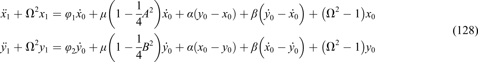
Ex8: Consider the following two coupled damped Van der Pol oscillators ⁶³

$$\begin{array}{l}\ddot{x}-\mu \left(1-x^2\right)\dot{x}+x=\alpha \left(y-x\right)+\beta \left(\dot{y}-\dot{x}\right),\\ \ddot{y}-\mu \left(1-y^2\right)\dot{y}+y=\alpha \left(x-y\right)+\beta \left(\dot{x}-\dot{y}\right)\end{array}$$

(123)

where $\mu ,\alpha ,\text{and }\beta$ are constants. This system is subjected to the following initial conditions

$$x\left(0\right)=A,\dot{x}\left(0\right)=0,y\left(0\right)=B\&\dot{y}\left(0\right)=0$$

(124)

Suppose that the above system has a common frequency $\Omega$ to be determined. Therefore, the corresponding homotopy system can be established in the form

$$\begin{array}{c}\ddot{x}+{\Omega }^{2}x=\rho \left[\mu \left(1-x^2\right)\dot{x}+\alpha \left(y-x\right)+\beta \left(\dot{y}-\dot{x}\right)+\left({\Omega }^2-1\right)x\right],\\ \ddot{y}+{\Omega }^{2}y=\rho \left[\mu \left(1-y^2\right)\dot{y}+\alpha \left(x-y\right)+\beta \left(\dot{x}-\dot{y}\right)+\left({\Omega }^2-1\right)y\right];\hspace{1em}\rho \in \left[\mathrm{0,1}\right]\end{array}$$

(125)

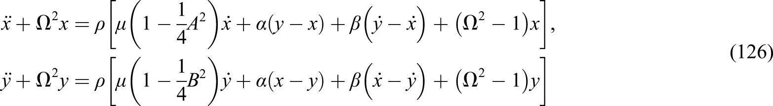
As mentioned before, the above nonlinear system can be converted to its corresponding linear one to facilitate the homotopy perturbation analysis, which leads to catching the exact solution. The converted system will arise through replacing $x^2$ and $y^2$ by $\left(1/4\right)A^2$ and $\left(1/4\right)B^2$ , respectively. The results are

$$\begin{array}{l}\ddot{x}+{\Omega }^{2}x=\rho \left[\mu \left(1-\frac{1}{4}{A}^2\right)\dot{x}+\alpha \left(y-x\right)+\beta \left(\dot{y}-\dot{x}\right)+\left({\Omega }^2-1\right)x\right],\\ \ddot{y}+{\Omega }^{2}y=\rho \left[\mu \left(1-\frac{1}{4}{B}^2\right)\dot{y}+\alpha \left(x-y\right)+\beta \left(\dot{x}-\dot{y}\right)+\left({\Omega }^2-1\right)y\right]\end{array}$$

(126)

Employing the system (112) into the system (126) and setting all identical powers in each equation to zero, we have

$$x_0\left(t\right)=A\cos \Omega t,\hspace{1em}{y}_0\left(t\right)=B\cos \Omega t$$

(127)

The system of the first-order problem is

$$\begin{array}{l}{\ddot{x}}_1+{\Omega }^2{x}_1={\phi }_1{\dot{x}}_0+\mu \left(1-\frac{1}{4}{A}^2\right){\dot{x}}_0+\alpha \left(y_0-x_0\right)+\beta \left({\dot{y}}_0-{\dot{x}}_0\right)+\left({\Omega }^2-1\right)x_0\\ {\ddot{y}}_1+{\Omega }^2{y}_1={\phi }_2{\dot{y}}_0+\mu \left(1-\frac{1}{4}{B}^2\right){\dot{y}}_0+\alpha \left(x_0-y_0\right)+\beta \left({\dot{x}}_0-{\dot{y}}_0\right)+\left({\Omega }^2-1\right)y_0\end{array}$$

(128)

Inserting the system of the zero-order solution into (128) and removing the secular terms requires

$${\Omega }^2-\left(1+\alpha \right)=-\frac{A}{B}\alpha ,\hspace{1em}\&\hspace{1em}{\Omega }^2-\left(1+\alpha \right)=-\frac{B}{A}\alpha$$

(129)

$${\phi }_1=\mu \left(1-\frac{1}{4}{A}^2\right)-\beta \left(1-\frac{B}{A}\right),\hspace{1em}\&\hspace{1em}{\phi }_2=\mu \left(1-\frac{1}{4}{B}^2\right)-\beta \left(1-\frac{A}{B}\right)$$

(130)

To obtain the frequency formulation, from equation (129), we have

$${\Omega }^2=1+\frac{3}{2}\alpha \hspace{0.17em}or\hspace{0.17em}{\Omega }^2=1+\frac{1}{2}\alpha$$

(131)

Replacing the two ratios $B/A$ and $A/B$ from the decaying parameters ${\phi }_1$ and ${\phi }_2$ with the help of (129) and (131) yields

$${\phi }_1=\mu \left(1-\frac{1}{4}{A}^2\right)-\frac{3}{2}\beta \hspace{1em}or\hspace{1em}{\phi }_1=\mu \left(1-\frac{1}{4}{A}^2\right)-\frac{1}{2}\beta$$

(132)

$${\phi }_2=\mu \left(1-\frac{1}{4}{B}^2\right)-\frac{3}{2}\beta ,\hspace{1em}or\hspace{1em}{\phi }_2=\mu \left(1-\frac{1}{4}{B}^2\right)-\frac{1}{2}\beta$$

(133)

Where the first order solutions have vanished, then the perturbed solutions are, only, the zero solutions given in (127). Therefore, substituting (127) into (126) and using (130), to produce the following exact solutions

$$x\left(t\right)=A{e}^{\left(1/2\right)t\left(\mu \left(1-\left(1/4\right)A^2\right)-\left(3/2\right)\beta \right)}\cos t\sqrt{1+\frac{3}{2}\alpha },\hspace{1em}y\left(t\right)=B{e}^{\left(1/2\right)t\left(\mu \left(1-\left(1/4\right)B^2\right)-\frac{3}{2}\beta \right)}\cos t\sqrt{1+\frac{3}{2}\alpha }$$

(134)

$$\text{Or}\hspace{0.17em}x\left(t\right)=A{e}^{\left(1/2\right)t\left(\mu \left(1-\left(1/4\right)A^2\right)-\left(1/2\right)\beta \right)}\cos t\sqrt{1+\frac{1}{2}\alpha },\hspace{1em}y\left(t\right)=B{e}^{\left(1/2\right)t\left(\mu \left(1-\left(1/4\right)B^2\right)-\left(1/2\right)\beta \right)}\cos t\sqrt{1+\frac{1}{2}\alpha }$$

(135)

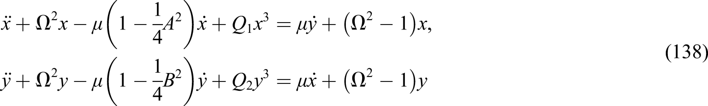
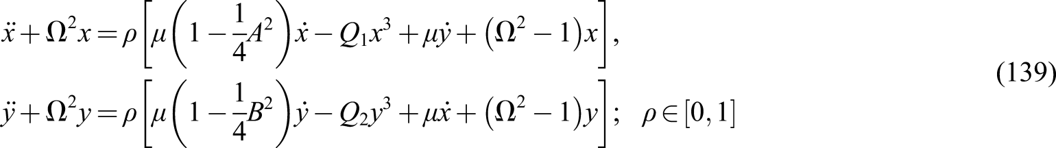
Ex9: The system of two coupled Van der Pol oscillators is one of the canonical models exhibiting the mutual synchronization behavior. ⁶⁴ Consider the following coupled Duffing–Van der Pol oscillator

$$\begin{array}{c}\ddot{x}-\mu \left(1-x^2\right)\dot{x}+x+Q_1{x}^3=\mu \dot{y},\\ \ddot{y}-\mu \left(1-y^2\right)\dot{y}+y+Q_2{y}^3=\mu \dot{x}\end{array}$$

(136)

where $\mu$ , $Q_1$ , and $Q_2$ are constants. Consider that this system has initial conditions

$$x\left(0\right)=A,\dot{x}\left(0\right)=0,y\left(0\right)=B\&\dot{y}\left(0\right)=0$$

(137)

Introducing the common-conservative frequency $\Omega$ and using the simplification given in the above examples into the system (136) becomes

$$\begin{array}{l}\ddot{x}+{\Omega }^{2}x-\mu \left(1-\frac{1}{4}{A}^2\right)\dot{x}+Q_1{x}^3=\mu \dot{y}+\left({\Omega }^2-1\right)x,\\ \ddot{y}+{\Omega }^{2}y-\mu \left(1-\frac{1}{4}{B}^2\right)\dot{y}+Q_2{y}^3=\mu \dot{x}+\left({\Omega }^2-1\right)y\end{array}$$

(138)

Construct the homotopy system in the form

$$\begin{array}{l}\ddot{x}+{\Omega }^{2}x=\rho \left[\mu \left(1-\frac{1}{4}{A}^2\right)\dot{x}-Q_1{x}^3+\mu \dot{y}+\left({\Omega }^2-1\right)x\right],\\ \ddot{y}+{\Omega }^{2}y=\rho \left[\mu \left(1-\frac{1}{4}{B}^2\right)\dot{y}-Q_2{y}^3+\mu \dot{x}+\left({\Omega }^2-1\right)y\right];\hspace{1em}\rho \in \left[\mathrm{0,1}\right]\end{array}$$

(139)

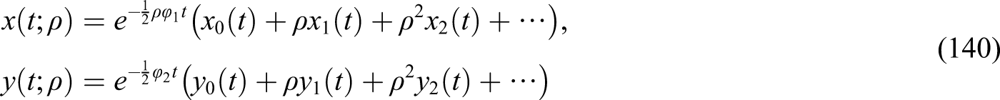
Consider the suggested solutions are performed as

$$\begin{array}{l}x\left(t;\rho \right)=e^{-\frac{1}{2}\hspace{0.17em}\rho {\phi }_{1}t}\left(x_0\left(t\right)+\rho x_1\left(t\right)+{\rho }^2{x}_2\left(t\right)+\cdots \right),\\ y\left(t;\rho \right)=e^{-\frac{1}{2}\hspace{0.17em}{\phi }_{2}t}\left(y_0\left(t\right)+\rho y_1\left(t\right)+{\rho }^2{y}_2\left(t\right)+\cdots \right)\end{array}$$

(140)

Employing (140) into (139), then arranging in powers of $\rho$ , and setting the identical powers to zero yield

$$x_0\left(t\right)=A\cos \Omega t,\hspace{1em}{y}_0\left(t\right)=B\cos \Omega t$$

(141)

The first-order system is

$$\begin{array}{l}{\ddot{x}}_1+{\Omega }^2{x}_1=\mu \left(1-\frac{1}{4}{A}^2\right){\dot{x}}_0-Q_1{x}_0^3+\mu {\dot{y}}_0+\left({\Omega }^2-1\right)x_0,\\ {\ddot{y}}_1+{\Omega }^2{y}_1=\mu \left(1-\frac{1}{4}{B}^2\right){\dot{y}}_0-Q_2{y}_0^3+\mu {\dot{x}}_0+\left({\Omega }^2-1\right)y_0\end{array}$$

(142)

Secular terms can be imposed when the zero-order solutions are inserted into the system (142). Removing the resulting secular terms requires that

$${\Omega }^2-1=-\frac{3}{4}{A}^2{Q}_1,\hspace{0.17em}\hspace{0.17em}\hspace{0.17em}\hspace{0.17em}\hspace{0.17em}{\Omega }^2-1=-\frac{3}{4}{B}^2{Q}_2,$$

(143)

$$\hspace{0.17em}\hspace{0.17em}{\phi }_1=\mu \left(1-\frac{1}{4}{A}^2\right)-\beta \left(1-\frac{B}{A}\right)\hspace{0.17em}\hspace{0.17em}\hspace{0.17em}\hspace{0.17em}\hspace{0.17em}\hspace{0.17em}\hspace{0.17em}\&\hspace{0.17em}\hspace{0.17em}\hspace{0.17em}\hspace{0.17em}\hspace{0.17em}{\phi }_2=\mu \left(1-\frac{1}{4}{B}^2\right)-\beta \left(1-\frac{A}{B}\right).$$

(144)

It can be read, from the two solvability conditions (143), that there is a relationship between the two amplitudes $A$ and $B$ . That is

$$\frac{A}{B}=\pm \sqrt{\frac{Q_2}{Q_1}}$$

(145)

Employing (145) with (143), the frequency equation is found in the form

$${\Omega }^2=1\pm \frac{3}{4}AB\sqrt{Q_1{Q}_2}$$

(146)

Solution of the first-order system without secular terms gives

$$\begin{array}{l}{x}_1=\frac{1}{32{\Omega }^2}{A}^3{Q}_1\left(\cos 3\Omega t-\cos \Omega t\right),\\ y_1=\frac{1}{32{\Omega }^2}{B}^3{Q}_2\left(\cos 3\Omega t-\cos \Omega t\right)\end{array}$$

(147)

Inserting (141) and (147) into (140) and letting $\rho \to 1$ lead to

$$\begin{array}{l}x\left(t\right)=A{e}^{-\frac{1}{2}{\phi }_{1}t}\left(\cos \Omega t+\frac{1}{32{\Omega }^2}{A}^2{Q}_1\left(\cos 3\Omega t-\cos \Omega t\right)\right),\\ y\left(t\right)=B{e}^{-\frac{1}{2}{\phi }_{2}t}\left(\cos \Omega t+\frac{1}{32{\Omega }^2}{B}^2{Q}_2\left(\cos 3\Omega t-\cos \Omega t\right)\right)\end{array}$$

(148)

where ${\phi }_1,{\phi }_2$ , and $\Omega$ are given by (144) and (146), respectively.

Ex10: Consider the following generalized Van der Pol type oscillator ⁶⁵

$$\ddot{y}+a_1\dot{y}+a_{0}y+a_2{y}^3+a_3\dot{y}{y}^2+a_{4}y{\dot{y}}^2+a_5{\dot{y}}^3=0;\hspace{1em}y\left(0\right)=A,\hspace{1em}\dot{y}\left(0\right)=0$$

(149)

The homotopy equation is

$$\ddot{y}+a_{0}y+\rho \left[\left(a_1+a_3{y}^2+a_5{\dot{y}}^2\right)\dot{y}+a_2{y}^3+a_{4}y{\dot{y}}^2\right]=0;\hspace{0.17em}\hspace{0.17em}\hspace{0.17em}\rho \in \left[\mathrm{0,1}\right]$$

(150)

Considering the frequency analysis so that we define the following frequency expansion

$${\Omega }^2=a_0+\rho {\Omega }_1+{\rho }^2{\Omega }_2+\cdots$$

(151)

Assuming that the function $y\left(t;\rho \right)$ has been expanded as

$$y\left(t;\rho \right)=e^{-\rho \phi t}\left(y_0\left(t\right)+\rho y_1\left(t\right)+{\rho }^2{y}_2\left(t\right)+\cdots \right)$$

(152)

Employing (151) and (152) with (150) and equating the identical powers of $\rho$ to zero yield

$${\rho }^0:{\ddot{y}}_0+{\Omega }^2{y}_0=0,y_0\left(0\right)=A,{\dot{y}}_0\left(0\right)=0$$

(153)

$${\rho }^1:{\ddot{y}}_1+{\Omega }^2{y}_1=\left({\Omega }_1-a_2{y}_0^2-a_4{\dot{y}}_0^2\right)y_0+2\phi {\dot{y}}_0-\left(a_1+a_3{y}_0^2+a_5{\dot{y}}_0^2\right){\dot{y}}_0,y_1\left(0\right)=0,{\dot{y}}_1\left(0\right)=0$$

(154)

Solution of the zero-order problem leads to

$$y_0\left(t\right)=A\cos \Omega t$$

(155)

Substituting (155) into (154), the requirement of no secular term in $y_1\left(t\right)$ needs

$${\Omega }_1=\frac{1}{4}{A}^2\left(3a_2+a_4{\Omega }^2\right)$$

(156)

and

$$\phi =\frac{1}{2}{a}_1-\frac{1}{8}\left(a_3+3a_5{\Omega }^2\right)A^2$$

(157)

Solution of (154) without secular terms becomes

$$y_1\left(t\right)=-\frac{A^3}{32{\Omega }^2}\left[\left(a_4{\Omega }^2-a_2\right)\left(\cos 3\Omega t-\cos \Omega t\right)+\Omega \left(a_3-a_5{\Omega }^2\right)\left(\sin 3\Omega t-3\sin \Omega t\right)\right]$$

(158)

If the first-order approximation is enough, then setting $\rho \to 1$ in the expansions (151) and (152) yields the approximate solution and the frequency, respectively

$${\Omega }^2=\frac{a_0+\left(3/4\right)a_2{A}^2}{1-\left(1/4\right)a_4{A}^2}$$

(159)

$$y\left(t\right)=A{e}^{-\left(1/2\right)\left(a_1-\left(1/4\right)\left(a_3+3a_5{\Omega }^2\right)A^2\right)t}\left\{\cos \Omega t-\frac{A^2}{32{\Omega }^2}\left[\left(a_4{\Omega }^2-a_2\right)\left(\cos 3\Omega t-\cos \Omega t\right)+\Omega \left(a_3-a_5{\Omega }^2\right)\left(\sin 3\Omega t-3\sin \Omega t\right)\right]\right\}$$

(160)

It is observed that the above oscillation becomes in the form of the conservative behavior when

$${\Omega }^2=\frac{4a_1-a_3{A}^2}{3a_5{A}^2}$$

(161)

By combining (159) and (161), we show the periodic solution can occur only when the amplitude $A$ satisfies the following relation

$$\left(a_3{a}_4-9a_5{a}_2\right)A^4-4\left(a_3+a_4{a}_1+3a_0{a}_5\right)A^2+16a_1=0$$

(162)

Ex11: In the present example, we have developed a technique for obtaining the asymptotic solutions of third-order critically damped linear systems. Consider the following linear third-order damping oscillator^66,67

$$\stackrel{\dots }{y}\left(t\right)+P\ddot{y}\left(t\right)+\mu \dot{y}\left(t\right)+\sigma y\left(t\right)=0,y\left(0\right)=A,\dot{y}\left(0\right)=0\&\ddot{y}\left(0\right)=0$$

(163)

where $P,\hspace{0.17em}\mu$ , and $\sigma$ are constants.

This problem is a linear damping third-order equation and its exact solution can be obtained through the modified homotopy perturbation analysis. The exact solution will arise when the first-order solution vanishes so that the zero-order solution is the exact one.

To apply the homotopy perturbation technique, the frequency parameter will be introduced in the form ${\Omega }^{3}y$ and equation (163) is rewritten as

$$\left(D^2-\Omega D+{\Omega }^2\right)\left(D+\Omega \right)y+P\ddot{y}+\mu \dot{y}+\sigma y={\Omega }^{3}y$$

(164)

where $\Omega$ is the unknown frequency. Introducing a new variable U, which is defined as

$$\left(D+\Omega \right)y\left(t\right)=U\left(t\right)$$

(165)

Accordingly, we have

$$U\left(0\right)=\Omega y\left(0\right)+\dot{y}\left(0\right)=A\Omega ,\&\hspace{0.17em}\dot{U}\left(0\right)=\Omega \dot{y}\left(0\right)+\ddot{y}\left(0\right)=0$$

(166)

In view of equations (165) and (166), we can convert equation (164) into the form

$$\left(D^2+{\Omega }^2\right)U=\Omega \dot{U}-{\left(D+\Omega \right)}^{-1}\left(P{D}^2+\mu D+\sigma -{\Omega }^3\right)U$$

(167)

The third-order equation of equation (163) is now converted to the second-order partner. The homotopy equation is

$$\left(D^2+{\Omega }^2\right)U\left(t\right)=\rho \left[\Omega \dot{U}-{\left(D+\Omega \right)}^{-1}\left(P{D}^2+\mu D+\sigma -{\Omega }^3\right)U\right]$$

(168)

The solution is assumed to have the form

$$U\left(t;\rho \right)=e^{-\rho \phi t}\left(U_0\left(t\right)+\rho U_1\left(t\right)+{\rho }^2{U}_2\left(t\right)+\cdots \right)$$

(169)

By the standard solution process required by the homotopy perturbation method, we have

$$U_0\left(t\right)=A\Omega \cos \Omega t$$

(170)

and the equation for $U_1$ reads

$$\left(D^2+{\Omega }^2\right)U_1\left(t\right)=-\left(\Omega +2\phi \right){\dot{U}}_0+\frac{1}{D^2-{\Omega }^2}[\left({\Omega }^4-\sigma \Omega \right)U_0+\left(\sigma -\mu \Omega -{\Omega }^3\right){\dot{U}}_0+\left(\mu -P\Omega \right){\ddot{U}}_0\hspace{0.17em}+P{\stackrel{⃛}{U}}_0]$$

(171)

In view of equation (170), equation (171) becomes

$$\left(D^2+{\Omega }^2\right)U_1\left(t\right)=\frac{A}{2}\left(4{\Omega }^2\phi +\sigma -\mu \Omega +{\Omega }^3-P{\Omega }^2\right)\sin \Omega t-\frac{A}{2}\left({\Omega }^3-\sigma -\Omega \left(\mu -P\Omega \right)\right)\cos \Omega t$$

(172)

No secular term in $U_1$ requires

$${\Omega }^3+P{\Omega }^2-\mu \Omega -\sigma =0$$

(173)

$$\phi =\frac{P{\Omega }^2+\mu \Omega -{\Omega }^3-\sigma }{4{\Omega }^2}$$

(174)

The parameter $\phi$ can be simplified if ${\Omega }^3$ is eliminated with the help of (173) which becomes

$$\phi =\frac{1}{2{\Omega }^2}\left(P{\Omega }^2-\sigma \right)$$

(175)

At this end, the exact solution of equation (167) is that

$$U\left(t\right)=A\Omega e^{-\left(1/2{\Omega }^2\right)\left(P{\Omega }^2-\sigma \right)t}\cos \Omega t$$

(176)

To derive the full decay solution of equation (163), (176) is inserted into (165) and the resulting first-order linear equation is solved to yield

$$y\left(t\right)=\frac{A}{{\phi }^2-2\phi \Omega +2{\Omega }^2}\left[e^{-\Omega t}\left({\phi }^2-\phi \Omega +{\Omega }^2\right)+\Omega e^{-\phi t}\left(\left(\Omega -\phi \right)\cos \Omega t+\Omega \sin \Omega t\right)\right]$$

(177)

This happens to be the exact solution, showing the effectiveness of the modified homotopy perturbation method.

Homotopy perturbation method for fractional non-conservative oscillators

Fractional vibration has become a hot topic in both mathematics and vibration theory. One of the most effective analytical methods for fractional oscillators is the homotopy perturbation method.

Ex12: The fractional damping Duffing equation is described as^68,69

$$\ddot{y}+\mu D^{\alpha }y+{\omega }_0^{2}y+Q{y}^3=0;\hspace{1em}0<\alpha <1$$

(178)

where $\mu ,\hspace{0.17em}{\omega }_0^2$ , and $Q$ are constants. The fractional derivative obeys the definition of the Riemann–Liouville time-fractional derivative. The initial conditions are assumed to be $y\left(0\right)=A,\dot{y}\left(0\right)=0$ . Introducing the total frequency $\Omega$ into equation (178) so that he homotopy equation is

$$H\left(y;\rho \right)=\ddot{y}+{\Omega }^{2}y+\rho \left(\left({\omega }_0^2-{\Omega }^2\right)y+\mu D^{\alpha }y+Q{y}^3\right)=0$$

(179)

Express the suggested solution in the form

$$y\left(t;\rho \right)=e^{-\rho \phi t}\left(y_0\left(t\right)+\rho y_1\left(t\right)+{\rho }^2{y}_2\left(t\right)+\cdots \right)$$

(180)

Inserting (180) into (179) and proceeding what is required by the homotopy perturbation method, equation (179) becomes

$$H\left(y;\rho \right)=H_0\left(y_0\right)+\rho H_1\left(y_1,y_0\right)+{\rho }^2{H}_2\left(y_2,y_1,y_0\right)+\cdots =0$$

(181)

The estimation $H_n;n=\mathrm{0,1,2},\mathrm{...}$ becomes as follows

$$H_0\left(y_0\right)=\underset{\rho \to 0}{\lim }H\left(y;\rho \right)$$

(182)

$$H_1\left(y_1,y_0\right)=\underset{\rho \to 0}{\lim }\frac{\partial }{\partial \rho }H\left(y;\rho \right)$$

(183)

$$H_r\left(,y_r,\mathrm{...},y_1,y_0\right)=\frac{1}{r!}\underset{\rho \to 0}{\lim }\frac{{\partial }^r}{\partial {\rho }^r}H\left(y;\rho \right)$$

(184)

By setting $H_r=0;r=\mathrm{0,1,2},\mathrm{...}$ , we obtain a linear system. The zero-order problem is

$${\ddot{y}}_0+{\Omega }^2{y}_0=0,y_0\left(0\right)=A,{\dot{y}}_0\left(0\right)=0$$

(185)

The first-order problem has the form

$${\ddot{y}}_1+{\Omega }^2{y}_1=-\left({\omega }_0^2-{\Omega }^2\right)y_0-Q{y}_0^3+2\phi {\dot{y}}_0-\mu D^{\alpha }{y}_0,y_1\left(0\right)=0,{\dot{y}}_1\left(0\right)=0$$

(186)

Inserting the solution of equation (185) into equation (186) yields

$${\ddot{y}}_1+{\Omega }^2{y}_1=-A\left({\omega }_0^2-{\Omega }^2\right)\cos \Omega t-\frac{1}{4}{A}^{3}Q\left(3\cos \Omega t+\cos 3\Omega t\right)-2A\phi \Omega \sin \Omega t-\mu A{D}^{\alpha }\cos \Omega t$$

(187)

Employing the following fraction derivative of $\cos \Omega t$ into equation (187)

$$D^{\alpha }\cos \Omega t={\Omega }^{\alpha }\cos \left(\Omega t+\frac{1}{2}\pi \alpha \right)$$

(188)

Dropping the secular terms requires that

$${\Omega }^2={\omega }_0^2+\frac{3}{4}{A}^{2}Q-\mu {\Omega }^{\alpha }\cos \left(\frac{1}{2}\pi \alpha \right)$$

(189)

$$\phi =\frac{1}{2}\mu {\Omega }^{\alpha -1}\sin \left(\frac{1}{2}\pi \alpha \right)$$

(190)

The total solution of equation (187) without the secular terms has the form

$$y_1\left(t\right)=\frac{1}{32{\Omega }^2}{A}^{3}Q\left(\cos 3\Omega t-\cos \Omega t\right)$$

(191)

It is noted that the ordinary Duffing equation and its approximate solution can be obtained in the limit case as α→1.

The final first-order approximate solution reads

$$y\left(t\right)=A{e}^{-\left(1/2\right)t\mu {\Omega }^{\alpha -1}\sin \left(\left(1/2\right)\pi \alpha \right)}\left(\cos \Omega t+\frac{1}{32{\Omega }^2}{A}^{2}Q\left(\cos 3\Omega t-\cos \Omega t\right)\right)$$

(192)

To enhance the solution and the frequency formula, we may select the decaying parameter $\phi$ , in the suggested solution (180), to be equal $\left(1/2\right)\mu$ , and the approximate solution (192) becomes

$$y\left(t\right)=A{e}^{-\left(1/2\right)\mu t}\left(\cos \Omega t+\frac{1}{32{\Omega }^2}{A}^{2}Q\left(\cos 3\Omega t-\cos \Omega t\right)\right)$$

(193)

Also, the solvability condition (190) becomes

$$1={\Omega }^{\alpha -1}\sin \left(\frac{1}{2}\pi \alpha \right)$$

(194)

Removing ${\Omega }^{\alpha }$ from the solvability condition (189) with the help of (194) yields the following frequency formula

$${\Omega }^2+\mu \cot \left(\frac{1}{2}\pi \alpha \right)\Omega -\left({\omega }_0^2+\frac{3}{4}{A}^{2}Q\right)=0$$

(195)

Ex13: Consider the following fractional Van der Pol oscillator ⁷⁰

$$\ddot{y}-\mu \left(1-y^2\right)D^{\alpha }y+y=0,\hspace{1em}0<\alpha <1$$

(196)

where $\mu >0$ is the coefficient of the damping coefficient. The initial conditions are selected to be y(0) = A and ẏ(0) = 0.

As mentioned before, equation (196) can be transformed to the linearized form by replacing $y^2$ to become $\left(1/4\right)A^2$ ; then we have a harmonic linear second-order equation with a fractional damping term

$$\ddot{y}-\mu \left(1-\frac{1}{4}{A}^2\right)D^{\alpha }y+y=0$$

(197)

Introducing the total frequency $\Omega$ for the system under consideration and establishing the corresponding homotopy equation in the form

$$\ddot{y}+{\Omega }^{2}y=\rho \left(\mu \left(1-\frac{1}{4}{A}^2\right)D^{\alpha }y+\left({\Omega }^2-1\right)y\right);\hspace{1em}\rho \in \left[\mathrm{0,1}\right]$$

(198)

Inserting the expansion (180) into (198), the zero-order solution has the form

$$y_0\left(t\right)=A\cos \Omega t$$

(199)

Employing (199) into (198) and dropping the secular terms yields

$${\Omega }^2-1+\mu \left(1-\frac{1}{4}{A}^2\right){\Omega }^{\alpha }\cos \left(\frac{1}{2}\pi \alpha \right)=0$$

(200)

$$2\phi =-\mu \left(1-\frac{1}{4}{A}^2\right){\Omega }^{\alpha -1}\sin \left(\frac{1}{2}\pi \alpha \right)$$

(201)

Because equation (198) is a linear equation, the first-order solution is $y_1\left(t\right)=y_2\left(t\right)=\cdots =y_n\left(t\right)=0$ . Accordingly, the zero-order solution represents the exact solution of equation (4). To find the frequency formulation, we set $\phi =\left(1/2\right)\mu \left(1-\left(1/4\right)A^2\right)$ , and from equations (200) and (201), we have

$${\Omega }^2-\mu \left(1-\frac{1}{4}{A}^2\right)\Omega \cot \left(\frac{1}{2}\pi \alpha \right)-1=0$$

(202)

So the exact solution becomes

$$y\left(t\right)=A{e}^{\left(1/2\right)\mu \left(1-\left(1/4\right)A^2\right)t}\cos \Omega t$$

(203)

The homotopy perturbation method for delay non-conservative oscillators

Ex14: Consider the following delayed Duffing equation ⁷¹

$$\ddot{y}+\mu \dot{y}\left(t-\tau \right)+{\omega }_0^{2}y+Q{y}^3=0;\hspace{1em}y\left(0\right)=A,\hspace{1em}\dot{y}\left(0\right)=0$$

(204)

The Duffing oscillator is given by the special case $\tau =0$ of the second-order pendulum equation.

The homotopy equation is

$$\ddot{y}+{\Omega }^{2}y+\rho \left(\mu \dot{y}\left(t-\tau \right)+\left({\omega }_0^2-{\Omega }^2\right)y+Q{y}^3\right)=0;\hspace{1em}\rho \in \left[\mathrm{0,1}\right]$$

(205)

Substituting the expansion (180) into equation (205) and setting the identical powers of $\rho$ to zero yields the solution of the zero-order problem has the form

$$y_0\left(t\right)=A\cos \Omega t$$

(206)

Accordingly, we have

$${\dot{y}}_0\left(t-\tau \right)=-A\Omega \left(\sin \Omega t\cos \Omega \tau -\cos \Omega t\sin \Omega \tau \right)$$

(207)

The first-order problem is given by

$${\ddot{y}}_1+{\Omega }^2{y}_1=2\phi {\dot{y}}_0-\mu {\dot{y}}_0\left(t-\tau \right)-\left({\omega }_0^2-{\Omega }^2\right)y_0-Q{y}_0^3$$

(208)

Inserting (206) and (207) into (208) and removing secular terms requires that

$${\Omega }^2-\left({\omega }_0^2+\frac{3}{4}{A}^{2}Q\right)=\mu \Omega \sin \Omega \tau ,\text{and}$$

(209)

$$\phi =\frac{1}{2}\mu \cos \Omega \tau$$

(210)

Solution of equation (208) free of the secular terms is

$$y_1\left(t\right)=\frac{1}{32{\Omega }^2}{A}^{3}Q\left(\cos 3\Omega t-\cos \Omega t\right)$$

(211)

The first approximate solution is

$$y\left(t\right)=A{e}^{-\left(1/2\right)t\mu \cos \Omega \tau }\left(\cos \Omega t+\frac{1}{32{\Omega }^2}{A}^{2}Q\left(\cos 3\Omega t-\cos \Omega t\right)\right)$$

(212)

It is noted that when the decay parameter $\phi$ , in the expansion (180), has been replaced by the value of the delay parameter $\tau$ , then (210) becomes

$$2\tau \hspace{0.17em}\Omega =\Omega \mu \hspace{0.17em}\cos \Omega \tau$$

(213)

In addition, the final solution (212) becomes

$$y\left(t\right)=A{e}^{-\tau t}\left(\cos \Omega t+\frac{1}{32{\Omega }^2}{A}^{2}Q\left(\cos 3\Omega t-\cos \Omega t\right)\right)$$

(214)

For the delayed Duffing oscillator (204), stability of large amplitude is rapidly oscillating periodic solutions.

The frequency formula can be obtained free of the harmonic functions of $\tau$ . In view of equations (213) and (209), the following frequency–amplitude equation is obtained

$${\Omega }^4-2\left({\omega }_0^2+\frac{3}{4}{A}^{2}Q+\frac{1}{2}{\mu }^2-2{\tau }^2\right){\Omega }^2+{\left({\omega }_0^2+\frac{3}{4}{A}^{2}Q\right)}^2=0$$

(215)

It is observed that the solution (214) will oscillate when

$${\mu }^2>4{\tau }^2,\text{and}$$

(216)

$${\omega }_0^2+\frac{3}{4}{A}^{2}Q+\frac{1}{2}{\mu }^2-2{\tau }^2>0$$

(217)

Ex15: Given the delay Van der Pol oscillator ⁷²

$$\ddot{y}+y-\mu \left(1-y^2\right)\dot{y}=\eta \dot{y}\left(t-\tau \right)\hspace{0.17em}y\left(0\right)=A,\hspace{0.17em}\hspace{0.17em}\hspace{0.17em}\dot{y}\left(0\right)=0,$$

(218)

where $\mu$ and $\eta$ are positive coefficients and $\tau$ is the time-delay parameter.

Equation (218) can be simplified to be

$$\ddot{y}+y-\mu \left(1-\frac{1}{4}{A}^2\right)\dot{y}=\eta \dot{y}\left(t-\tau \right)$$

(219)

Introducing the non-conservative frequency $\Omega$ and building the homotopy equation in the form

$$\ddot{y}+{\Omega }^{2}y=\rho \left[\mu \left(1-\frac{1}{4}{A}^2\right)\dot{y}+\eta \dot{y}\left(t-\tau \right)+\left({\Omega }^2-1\right)y\right]:\hspace{1em}\rho \in \left[\mathrm{0,1}\right]$$

(220)

Express the suggested solution given by (180), where $y_0\left(t\right)$ and $y_1\left(t\right)$ are, respectively, given by

$$y_0\left(t\right)=A\cos \Omega t$$

(221)

$${\ddot{y}}_1+{\Omega }^2{y}_1=2\phi {\dot{y}}_0+\mu \left(1-\frac{1}{4}{A}^2\right){\dot{y}}_0+\eta {\dot{y}}_0\left(t-\tau \right)+\left({\Omega }^2-1\right)y_0$$

(222)

Inserting (221) into (222) becomes

$${\ddot{y}}_1+{\Omega }^2{y}_1=A\left[\left({\Omega }^2-1\right)+\Omega \eta \sin \Omega \tau \right]\cos \Omega t-A\Omega \left[2\phi +\mu \left(1-\frac{1}{4}{A}^2\right)+\eta \cos \Omega \tau \right]\sin \Omega t$$

(223)

Removing secular terms requires

$${\Omega }^2-1=-\Omega \eta \sin \Omega \tau$$

(224)

$$\phi =-\frac{1}{2}\mu \left(1-\frac{1}{4}{A}^2\right)-\frac{1}{2}\eta \cos \Omega \tau$$

(225)

Due to the vanishing of $y_1$ , the solution (221) becomes the exact solution which is

$$y\left(t\right)=A{e}^{\left(1/2\right)t\left(\mu \left(1-\left(1/4\right)A^2\right)+\eta \cos \Omega \tau \right)}\cos \Omega t$$

(226)

To relax the frequency equation without using the Taylor expansion, we may be assuming that the decay parameter $\phi$ in (180) becomes $\tau$ and then the solvability (225) should be changed to become

$$\left[2\tau +\mu \left(1-\frac{1}{4}{A}^2\right)\right]\Omega =-\eta \Omega \cos \Omega \tau$$

(227)

Accordingly, the solution (226) becomes

$$y\left(t\right)=A{e}^{-\tau t}\cos \Omega t$$

(228)

By squaring each of (224) and (227) and adding yields

$${\Omega }^4-\left\{{\left[2\tau +\mu \left(1-\frac{1}{4}{A}^2\right)\right]}^2-{\eta }^2+2\right\}{\Omega }^2+1=0$$

(229)

Ex16: Consider the following linear third-order delay damping oscillator^61,73

$$\stackrel{\dots }{y}\left(t\right)+P\ddot{y}\left(t\right)+\mu \dot{y}\left(t\right)+\sigma y\left(t\right)=\eta \dot{y}\left(t-\tau \right)+\lambda y\left(t-\tau \right),y\left(0\right)=A,\dot{y}\left(0\right)=0\&\ddot{y}\left(0\right)=0$$

(230)

where $P,\hspace{0.17em}\mu$ , and $\sigma$ are constants.

To apply the homotopy perturbation technique, the frequency parameter will be introduced in the form ${\Omega }^{3}y$ and equation (230) is rewritten as

$$\left(D^2-\Omega D+{\Omega }^2\right)\left(D+\Omega \right)y+P\ddot{y}+\mu \dot{y}+\sigma y={\Omega }^{3}y+\eta \dot{y}\left(t-\tau \right)+\lambda y\left(t-\tau \right)$$

(231)

By the following transform

$$\left(D+\Omega \right)y\left(t\right)=U\left(t\right)$$

(232)

we have

$$U\left(0\right)=\Omega y\left(0\right)+\dot{y}\left(0\right)=A\Omega ,\hspace{1em}\&\hspace{1em}\dot{U}\left(0\right)=\Omega \dot{y}\left(0\right)+\ddot{y}\left(0\right)=0$$

(233)

Equation (231) is converted to the form

$$\left(D^2+{\Omega }^2\right)U=\Omega \dot{U}-{\left(D+\Omega \right)}^{-1}\left[\left(P{D}^2+\mu D+\sigma -{\Omega }^3\right)U+\left(\eta D+\lambda \right)U\left(t-\tau \right)\right]$$

(234)

The homotopy equation is

$$\left(D^2+{\Omega }^2\right)U\left(t\right)=\rho \left\{\Omega \dot{U}-{\left(D+\Omega \right)}^{-1}\left[\left(P{D}^2+\mu D+\sigma -{\Omega }^3\right)U+\left(\eta D+\lambda \right)U\left(t-\tau \right)\right]\right\};\hspace{1em}\rho \in \left[\mathrm{0,1}\right]$$

(235)

Express the non-conservative homotopy expansion as

$$U\left(t;\rho \right)=e^{-\rho \phi t}\left(U_0\left(t\right)+\rho U_1\left(t\right)+{\rho }^2{U}_2\left(t\right)+\cdots \right)$$

(236)

Employing (236) into the homotopy equation (235) and setting the coefficient of the identical powers of $\rho$ to zero yields the first two terms of (236) in the following form:

The zero-order equation has the solution

$$U_0\left(t\right)=A\Omega \cos \Omega t$$

(237)

$$U_0\left(t-\tau \right)=A\Omega \cos \Omega \left(t-\tau \right)$$

(238)

The equation for $U_1$ reads

$$\begin{array}{l}\left(D^2+{\Omega }^2\right)U_1\left(t\right)=-\left(\Omega +2\phi \right){\dot{U}}_0+\frac{1}{D^2-{\Omega }^2}\{\left[P{D}^2+\left({\Omega }^4-\sigma \Omega \right)+\left(\sigma -\mu \Omega -{\Omega }^3\right)D+\left(\mu -P\Omega \right)D^2\right]U_0\left(t\right)\\ +\left(\lambda \Omega +\left(\eta \Omega -\lambda \right)D-\eta D^2\right)U_0\left(t-\tau \right)\}\end{array}$$

(239)

Inserting (237) and (238) into (239) reduces to

$$\begin{array}{l}\left(D^2+{\Omega }^2\right)U_1\left(t\right)=\frac{1}{2}A\left[\left(\lambda +\eta \Omega \right)\cos \Omega \tau -\left(\lambda -\eta \Omega \right)\sin \Omega \tau +{\Omega }^3+P{\Omega }^2-\mu \Omega -\sigma \right]\cos \Omega t\\ +\frac{1}{2}A\left[4{\Omega }^2\phi -\left(\lambda -\eta \Omega \right)\cos \Omega \tau -\left(\lambda +\eta \Omega \right)\sin \Omega \tau +{\Omega }^3-P{\Omega }^2-\mu \Omega +\sigma \right]\sin \Omega \end{array}$$

(240)

The no secular term assumption requires

$${\Omega }^3+P{\Omega }^2-\mu \Omega -\sigma =-\left(\lambda +\eta \Omega \right)\cos \Omega \tau +\left(\lambda -\eta \Omega \right)\sin \Omega \tau$$

(241)

$$\phi =\frac{1}{4{\Omega }^2}\left[-\sigma +\mu \Omega +P{\Omega }^2-{\Omega }^3+\left(\lambda -\eta \Omega \right)\cos \Omega \tau +\left(\lambda +\eta \Omega \right)\sin \Omega \tau \right]$$

(242)

Under these conditions, $U_1\equiv 0$ , and $U_0$ is the exact solution for equation (235)

$$U\left(t\right)=U_0\left(t\right)=A\Omega e^{-\phi t}\cos \Omega t$$

(243)

In view of equations (241) and (242), $\phi$ is simplified as

$$\phi =\frac{1}{2{\Omega }^2}\left(P{\Omega }^2-\sigma +\lambda \cos \Omega \tau +\eta \Omega \sin \Omega \tau \right)$$

(244)

In view of equation (243), from equation (232), we obtain the solution of equation (230), which is

$$y\left(t\right)=\frac{A}{{\phi }^2-2\phi \Omega +2{\Omega }^2}\left[e^{-\Omega t}\left({\phi }^2-\phi \Omega +{\Omega }^2\right)+\Omega e^{-\phi t}\left(\left(\Omega -\phi \right)\cos \Omega t+\Omega \sin \Omega t\right)\right]$$

(245)

The frequency formulation given in equation (241) is expressed in an inexplicit form. In order to have an explicit one, we introduce an artificial parameter in equation (241)

$${\Omega }^3+P{\Omega }^2-\mu \Omega -\sigma =\epsilon \left[-\left(\lambda +\eta \Omega \right)\cos \Omega \tau +\left(\lambda -\eta \Omega \right)\sin \Omega \tau \right];\hspace{1em}\epsilon \in \left[\mathrm{0,1}\right]$$

(246)

Expand the frequency $\Omega \left(\rho \right)$ as

$$\Omega \left(\rho \right)={\Omega }_0+\epsilon {\Omega }_1+{\epsilon }^2{\Omega }_2+\cdots$$

(247)

Employing (247) into (246), collecting the identical power of $\epsilon$ , and setting it to zero yield

$${\epsilon }^0:{\Omega }_0^3+P{\Omega }_0^2-\mu {\Omega }_0-\sigma =0$$

(248)

$${\epsilon }^1:{\Omega }_1=\frac{\left(\lambda -\eta {\Omega }_0\right)\sin {\Omega }_0\tau -\left(\lambda +\eta {\Omega }_0\right)\cos {\Omega }_0\tau }{\left(3{\Omega }_0^2+2P{\Omega }_0-\mu \right)}$$

(249)

Inserting the solution of (248) into (249) to have the following approximate value

$$\Omega ={\Omega }_0+\frac{\left(\lambda -\eta {\Omega }_0\right)\sin {\Omega }_0\tau -\left(\lambda +\eta {\Omega }_0\right)\cos {\Omega }_0\tau }{\left(3{\Omega }_0^2+2P{\Omega }_0-\mu \right)}$$

(250)

Ex17: Consider the following fractional damped Duffing oscillator with delay ⁵⁴

$$\ddot{y}\left(t\right)+\mu \dot{y}\left(t\right)+{\omega }_0^{2}y\left(t\right)+\eta D^{\alpha }y\left(t-\tau \right)+Q{y}^3\left(t\right)=0,\hspace{1em}0<\alpha <1$$

(251)

where $\mu ,\hspace{0.17em}\eta ,\hspace{0.17em}Q$ , and ${\omega }_0^2$ are real constant coefficients. This system is subjected to $y\left(0\right)=A,\hspace{1em}\dot{y}\left(0\right)=0$ . The nearness of $\alpha$ to zero into equation (251) and the Duffing oscillator having a displacement time-delayed are found. As α has become close to unity, the velocity time-delayed of the Duffing equation should be obtained.

We will use the frequency expansion technique and the modified homotopy expansion to derive an approximate solution for the given equation. According to the homotopy technique, we can formulate the following homotopy equation

$$\ddot{y}\left(t;\rho \right)+{\omega }_0^{2}y\left(t;\rho \right)+\rho \left(\mu \dot{y}+\eta D^{\alpha }y\left(t-\tau ;\rho \right)+Q{y}^3\left(t;\rho \right)\right)=0;\hspace{1em}\rho \in \left[\mathrm{0,1}\right]$$

(252)

Expand each of the natural frequency as

$${\omega }^2\left(\rho \right)={\omega }_0^2+\rho {\omega }_1+{\rho }^2{\omega }_2+\cdots$$

(253)

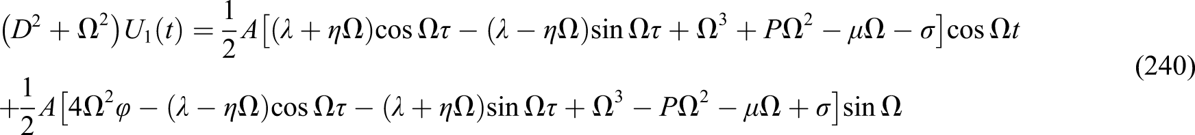
Employing (180) and (253) into (252), we get the equations at each order as

$${\ddot{y}}_0+{\omega }^2{y}_0=0;\hspace{1em}{y}_0\left(0\right)=A,{\dot{y}}_0\left(0\right)=0$$

(254)

$${\ddot{y}}_1+{\omega }^2{y}_1={\omega }_1{y}_0+2\phi {\dot{y}}_0-\left(\mu {\dot{y}}_0+\eta D^{\alpha }{y}_0\left(t-\tau \right)+Q{y}_0^3\right);\hspace{1em}{y}_1\left(0\right)=0,{\dot{y}}_1\left(0\right)=0$$

(255)

The solution of equation (254) is known to be

$$y_0\left(t\right)=A\cos \omega t$$

(256)

Accordingly, we have

$$y_0\left(t-\tau \right)=A\cos \omega \left(t-\tau \right)$$

(257)

Inserting (256) and (257) into (255) yields

$${\ddot{y}}_1+{\omega }^2{y}_1=\left(A{\omega }_1-\frac{3}{4}{A}^{3}Q\right)\cos \omega t+\omega A\left(\mu -2\phi \right)\sin \omega t-A\eta D^{\alpha }\cos \omega \left(t-\tau \right)-\frac{1}{4}{A}^{3}Q\cos 3\omega t;\hspace{1em}{y}_1\left(0\right)=0,\hspace{0.17em}{\dot{y}}_1\left(0\right)=0$$

(258)

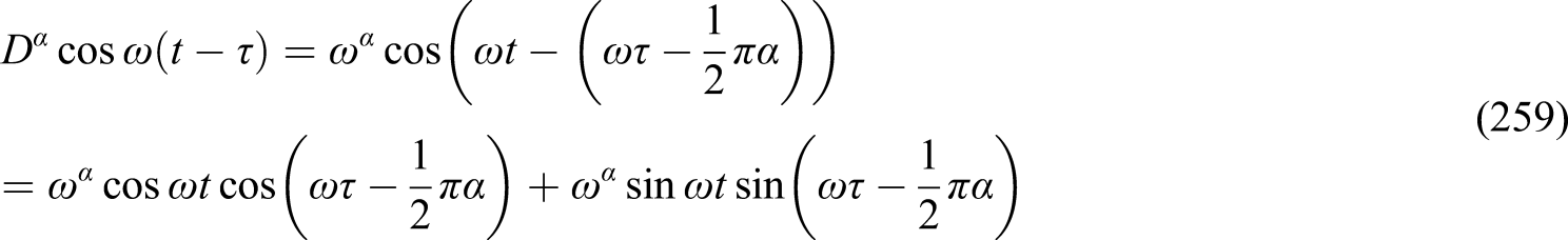
The fractional-order derivative of $y_0\left(t-\tau \right)$ , involved in equation (255), can be easily approximately established in the light of the fractional definition in the form

$$\begin{array}{l}{D}^{\alpha }\cos \omega \left(t-\tau \right)={\omega }^{\alpha }\cos \left(\omega t-\left(\omega \tau -\frac{1}{2}\pi \alpha \right)\right)\\ ={\omega }^{\alpha }\cos \omega t\cos \left(\omega \tau -\frac{1}{2}\pi \alpha \right)+{\omega }^{\alpha }\sin \omega t\sin \left(\omega \tau -\frac{1}{2}\pi \alpha \right)\end{array}$$

(259)

Substituting (259) into (258) and then dropping the secular terms yield

$${\omega }_1=\frac{3}{4}{A}^{2}Q+\eta {\omega }^{\alpha }\cos \left(\omega \tau -\frac{1}{2}\pi \alpha \right)$$

(260)

$$\phi =\frac{1}{2}\mu -\frac{1}{2}\eta {\omega }^{\alpha -1}\sin \left(\omega \tau -\frac{1}{2}\pi \alpha \right)$$

(261)

The uniform first-order solution is

$$y_1\left(t\right)=\frac{A^{3}Q}{32{\omega }^2}\left(\cos 3\omega t-\cos \omega t\right)$$

(262)

For the one iteration process, we insert (256) and (262) into (180) for letting $\rho \to 1$ yields

$$y\left(t\right)=A{e}^{-\left(1/2\right)t\left(\mu -\eta {\omega }^{\alpha -1}\sin \left(\omega \tau -\left(1/2\right)\pi \alpha \right)\right)}\left(\cos \omega t+\frac{A^{2}Q}{32{\omega }^2}\left(\cos 3\omega t-\cos \omega t\right)\right)$$

(263)

Similarly, we insert (260) into (253) and setting $\rho \to 1$ gets

$${\omega }^2-\left({\omega }_0^2+\frac{3}{4}{A}^{2}Q\right)=\eta {\omega }^{\alpha }\cos \left(\omega \tau -\frac{1}{2}\pi \alpha \right)$$

(264)

This is the frequency–amplitude relationship which depends on the time delay parameter $\tau$ and the order of the fractional parameter $\alpha$ . To establish the frequency–amplitude equation free of the harmonic functions, we may take the decaying parameter as the delay parameter $\tau$ . Therefore, (261) may be changed to be

$$\left(2\tau -\mu \right)\omega =-\eta {\omega }^{\alpha }\sin \left(\omega \tau -\frac{1}{2}\pi \alpha \right)$$

(265)

Also, the solution (263) becomes

$$y\left(t\right)=A{e}^{-\tau t}\left(\cos \omega t+\frac{A^{2}Q}{32{\omega }^2}\left(\cos 3\omega t-\cos \omega t\right)\right)$$

(266)

where the frequency $\omega$ can be estimated by squaring both (264) and (265) and adding yields

$${\omega }^4-\left[2\left({\omega }_0^2+\frac{3}{4}{A}^{2}Q\right)-{\left(2\tau -\mu \right)}^2\right]{\omega }^2+{\left({\omega }_0^2+\frac{3}{4}{A}^{2}Q\right)}^2={\eta }^2{\omega }^{2\alpha }$$

(267)

This frequency formulation can be directly used for practical applications.

Quasi-exact solution based on He’s frequency formula

There are alternative methods for nonlinear oscillators; some famous ones include the variational iteration method,^74–79 the exp-function method,^80–83 the variational theory,^82–84 the G’/G-expansion method, ⁸⁵ the Bayesian inference method, ⁸⁶ the barycentric rational interpolation collocation method, ⁸⁷ and others. ⁸⁸ This section focuses itself on a simple method to find the frequency–amplitude relationship of a nonlinear oscillator using He’s frequency formulation,^89–91 which represents a genius idea in converting a nonlinear equation into a linear equation. Since a linear equation often has a perfect solution, the solution of the linearized equation represents a near-perfect solution to the nonlinear equation, which is called a quasi-exact solution. However, dealing with a linear equation, whatever it is, is more accessible than dealing with a nonlinear equation.

Ex18: Consider the following oscillator of the Van der Pol type

$$\ddot{y}+\mu \left(1-\cos y\right)\dot{y}+f\left(y\right)=0;\hspace{1em}y\left(0\right)=A\&\dot{y}\left(0\right)=0$$

(268)

where the potential function $f\left(y\right)$ is defined as

$$f\left(y\right)={\displaystyle {\sum }_n{a}_n{y}^{2n+1}}$$

(269)

It is seen that the nonlinear damping term in equation (268) is a harmonic function. Without expanding this function, a difficulty will arise to analyze this equation by a perturbation technique. The suitable simple process to solve the above equation is using the non-perturbative approach.

Based on He’s frequency formula, equation (268) is rewritten approximately as

$$\ddot{y}+\mu \left(1-\cos y\right)\dot{y}+{\omega }^{2}y=0$$

(270)

where ${\omega }^2$ is estimated as

$${{\omega }^2=\frac{df}{dy}|}_{y=\left(1/2\right)A}={{\displaystyle {\sum }_n\left(2n+1\right)a_n{y}^{2n}}|}_{y=\left(1/2\right)A}={\displaystyle {\sum }_n\frac{\left(2n+1\right)}{2^{2n}}{a}_n{A}^{2n}}$$

(271)

Further, the nonlinear damping coefficient is evaluated as

$${\cos y|}_{y=\left(1/2\right)A}=\cos \left(\frac{1}{2}A\right)$$

(272)

Inserting (272) into equation (270) becomes

$$\ddot{y}+\mu \left(1-\cos \left(\frac{1}{2}A\right)\right)\dot{y}+{\omega }^{2}y=0$$

(273)

Now, equation (273) is a linear damping equation that is simpler than equation (268) where ${\omega }^2$ plays as a natural frequency. It is a solution having the exact form

$$y\left(t\right)=A{e}^{-\left(1/2\right)\mu \left(1-\cos \left(\left(1/2\right)A\right)\right)}\cos \Omega t$$

(274)

where the non-conservative frequency $\Omega$ is given by

$${\Omega }^2={\omega }^2-\frac{1}{4}{\mu }^2{\left(1-\cos \left(\frac{1}{2}A\right)\right)}^2$$

(275)

He’s frequency formula has been widely applied to various nonlinear vibration problems, for example, vibration systems in a microgravity condition,^92–94 3-D printing system, ⁹⁵ Fangzhu oscillator, ⁹⁶ the fractal cubic–quintic Duffing equation, ⁹⁷ the fractal Toda oscillator, ⁹⁸ and many modifications appeared in the literature.^99–101

Ex19: Solve the following fractional damping Duffing equation using He’s frequency formula ¹⁰²

$$D^{\alpha +1}y+\mu D^{\alpha }y+{\omega }_0^{2}y+Q{y}^3=0;\hspace{1em}y\left(0\right)=A,\hspace{1em}\dot{y}\left(0\right)=0;\hspace{1em}0<\alpha <1$$

(276)

In terms of the restoring force

$$f\left(y\right)={\omega }_0^{2}y+Q{y}^3$$

(277)

the fractional Duffing equation (276) becomes

$$D^{\alpha +1}y+\mu D^{\alpha }y+f\left(y\right)=0$$

(278)

Based on He’s frequency formula, equation (278) can be written in the form

$$D^{\alpha +1}y+\mu D^{\alpha }y+{\omega }^{2}y=0$$

(279)

where the Duffing frequency ${\omega }^2$ is estimated as ⁸⁶

$${\omega }^2={\frac{df}{dy}|}_{y=\left(1/2\right)A}={\omega }_0^2+\frac{3}{4}Q{A}^2$$

(280)

Now, equation (279) has a linear form with the fractional order. It can be solved using the modified homotopy technique. It is noted that the Duffing frequency ${\omega }^2$ will be used as a natural frequency for the linearized equation (279). Applying $\left(D^2+{\omega }^2\right){\left(D^{\alpha +1}+{\omega }^2\right)}^{-1}$ to both sides of equation (279), we have

$$\left(D^2+{\omega }^2\right)y+\mu {\left(D^{\alpha +1}+{\omega }^2\right)}^{-1}{D}^{\alpha }y=0$$

(281)

A homotopy equation is

$$\left(D^2+{\Omega }^2\right)y+\rho \left[\left({\omega }^2-{\Omega }^2\right)y+\mu {\left(D^{\alpha +1}+{\omega }^2\right)}^{-1}{D}^{\alpha }y\right]=0;\hspace{1em}\rho \in \left[\mathrm{0,1}\right]$$

(282)

By a similar operation, as shown above, we have

$$y_0=A\cos \Omega t$$

(283)

$$\left(D^2+{\Omega }^2\right)y_1=-\left({\omega }^2-{\Omega }^2\right)y_0+2\phi {\dot{y}}_0-\mu {\left(D^{\alpha +1}+{\omega }^2\right)}^{-1}{D}^{\alpha }{y}_0$$

(284)

It is noted that the following formulas are useful to use

$$D^{\alpha }\cos \Omega t={\Omega }^{\alpha }\cos \left(\Omega t+\frac{1}{2}\pi \alpha \right)$$

(285)

$${\left(D^{\alpha +1}+{\omega }^2\right)}^{-1}\cos \left(\Omega t+\frac{1}{2}\pi \alpha \right)=\frac{{\omega }^2\cos \left(\Omega t+\left(1/2\right)\pi \alpha \right)+{\Omega }^{\alpha +1}\sin \Omega t}{\left({\Omega }^{2\alpha +2}+{\omega }^4-2{\omega }^2{\Omega }^{\alpha +1}\sin \left(\pi \alpha /2\right)\right)}$$

(286)

Inserting (283) into (284) and using (285) and (286) yields

$$\left(D_t^2+{\Omega }^2\right)y_1=\left({\Omega }^2-{\omega }^2\right)A\cos \Omega t-2A\Omega \phi \sin \Omega t+A{\Omega }^{\alpha }\mu \frac{{\omega }^2\cos \left(\Omega t+\left(1/2\right)\pi \alpha \right)+{\Omega }^{\alpha +1}\sin \Omega t}{\left({\Omega }^{2\alpha +2}+{\omega }^4-2{\omega }^2{\Omega }^{\alpha +1}\sin \left(\left(1/2\right)\pi \alpha \right)\right)}$$

(287)

Dropping the secular terms requires

$${\Omega }^2={\omega }^2-\frac{{\Omega }^{\alpha }{\omega }^2\mu \cos \left(\left(1/2\right)\pi \alpha \right)}{\left({\Omega }^{2\alpha +2}+{\omega }^4-2{\omega }^2{\Omega }^{\alpha +1}\sin \left(\left(1/2\right)\pi \alpha \right)\right)}$$

(288)

$$\phi =\frac{\mu {\Omega }^{\alpha -1}\left({\Omega }^{\alpha +1}-{\omega }^2\sin \left(\left(1/2\right)\pi \alpha \right)\right)}{2\left({\Omega }^{2\alpha +2}+{\omega }^4-2{\omega }^2{\Omega }^{\alpha +1}\sin \left(\left(1/2\right)\pi \alpha \right)\right)}$$

(289)

Under the above conditions, $y_1\equiv 0$ so that $y_0$ is the exact solution for the linearized equation (279) which is given by

$$y\left(t\right)=y_0\left(t\right)=A{e}^{-\phi t}\cos \Omega t$$

(290)

This solution is called the quasi-exact solution of the original fractional Duffing equation.

Due to the complicated frequency formula (288), a perturbation technique can be used to get an approximation of it. Introduce a small parameter $\epsilon$ into (288) so that

$${\Omega }^2\left(\epsilon \right)={\omega }^2-\frac{\epsilon {\Omega }^{\alpha }{\omega }^2\mu \cos \left(\left(1/2\right)\pi \alpha \right)}{\left({\Omega }^{2\alpha +2}+{\omega }^4-2{\omega }^2{\Omega }^{\alpha +1}\sin \left(\left(1/2\right)\pi \alpha \right)\right)}$$

(291)

Expanded the frequency ${\Omega }^2\left(\epsilon \right)$ in the form

$${\Omega }^2\left(\epsilon \right)={\Omega }_0+\epsilon {\Omega }_1+{\epsilon }^2{\Omega }_2+\cdots$$

(292)

Inserting (292) into (291), the zero-order and the first-order of the frequency expansion are estimated to become

$${\Omega }_0={\omega }^2$$

(293)

$${\Omega }_1=-\frac{{\Omega }_0^{\alpha }{\omega }^2\mu \cos \left(\left(1/2\right)\pi \alpha \right)}{\left({\Omega }_0^{2\alpha +2}+{\omega }^4-2{\omega }^2{\Omega }_0^{\alpha +1}\sin \left(\left(1/2\right)\pi \alpha \right)\right)}$$

(294)

Employing (293) into (294) yields

$${\Omega }_1=-\frac{{\omega }^{2\alpha }\mu \cos \left(\left(1/2\right)\pi \alpha \right)}{{\omega }^2\left({\omega }^{4\alpha }+1-2{\omega }^{2\alpha }\sin \left(\left(1/2\right)\pi \alpha \right)\right)}$$

(295)

The first-order approximate frequency formula can be obtained as

$${\Omega }^2={\omega }^2-\frac{{\omega }^{2\alpha }\mu \cos \left(\left(1/2\right)\pi \alpha \right)}{{\omega }^2\left({\omega }^{4\alpha }+1-2{\omega }^{2\alpha }\sin \left(\left(1/2\right)\pi \alpha \right)\right)}$$

(296)

This approximate frequency can be used to estimate the decay parameter φ.

Conclusion

This work is focused on the analysis of the above-described examples for the non-conservative oscillators. As pointed out by D.D. Ganji in Science Watch on February 8, (2008), He’s perturbation method itself is mathematically beautiful and extremely accessible to non-mathematicians. This review article confirms this fact again, and the modification of the homotopy perturbation method has made the solution process for conservative oscillators extremely simple. In addition, we would also like to point out that our new modification is unique to HPM and that it does not exist in the other methods such as straightforward, Lindstedt–Poincare’ technique, multiple scales method, and others, and it can be used with these methods to address issues of the non-conservative oscillators, and it will give good results. This review article uses examples to show the basic ideas and the solution process and can be used as a paradigm for other applications.