Hybrid rayleigh–van der pol–duffing oscillator: Stability analysis and controller

Abstract

The current study examines the hybrid Rayleigh–Van der Pol–Duffing oscillator (HRVD) with a cubic–quintic nonlinear term and an external excited force. The Poincaré–Lindstedt technique is adapted to attain an approximate bounded solution. A comparison between the approximate solution with the fourth-order Runge–Kutta method (RK4) shows a good matching. In case of the autonomous system, the linearized stability approach is employed to realize the stability performance near fixed points. The phase portraits are plotted to visualize the behavior of HRVD around their fixed points. The multiple scales method, along with a nonlinear integrated positive position feedback (NIPPF) controller, is employed to minimize the vibrations of the excited force. Optimal conditions of the operation system and frequency response curves (FRCs) are discussed at different values of the controller and the system parameters. The system is scrutinized numerically and graphically before and after providing the controller at the primary resonance case. The MATLAB program is employed to simulate the effectiveness of different parameters and the controller on the system. The calculations showed that NIPPF is the best controller. The validations of time history and FRC of the analysis as well as the numerical results are satisfied by making a comparison among them.

Introduction

Nonlinear vibration provides an interesting potential example of the mathematical description of the nonlinear behavior of many phenomena in science, physics, and practical engineering; for example, the N/MEMS system vibrates nonlinearly.^1-7 The nonlinear wave equation of Kundu–Mukherjee–Naskar equation can be finally converted into a Duffing-like equation. ⁸ Fangzhou oscillator is a generalized Duffing equation (DE) with a singular term.^9-11 The nonlinear vibration systems in a porous medium can be converted to a fractal modification of the DE. ^12-14 The gecko-like vibration plays an important role in the accurate 3-D printing process. ¹⁵ The inherent pull-in instability of MEMS systems can be completely overcome by the fractal vibration theory.^16-18 The homotopy perturbation method (HPM) ¹⁹ and the Hamitonian approach ²⁰ are two main analytical tools for nonlinear vibration systems. The combination of the Laplace transforms, Lagrange multiplier, fractional complex transforms, and Mohand transform with HPM was employed to find approximate solutions for nonlinear partial differential equations.^21-25 Additionally, there are many other methods available in the literature.

Duffing equation is adopted in many problems such as optical stability, electrical circuit, oscillation of plasma, and the buckled beam. ²⁶ Nonlinear oscillations have been of paramount importance in practical engineering, physics, applied mathematics, and several real-world requirements for many years. Nayfeh ²⁷ and Mickens ²⁸ utilized different approaches to obtain approximate solutions for nonlinear oscillators. Moatimid ²⁹ combined the HPM and Laplace transform to obtain an approximate bounded solution for the parametric DE. This analysis resulted in an exact solution for the cubic DE and showed that the damped parameter and the cubic stiffness parameter have a destabilizing influence on the system. In the last decades, much research was devoted to examining the control of resonantly forced systems in several practical engineering areas. In the passive vibration absorbers, a physical practice is associated with primary organization, whereas in case of active absorbers, the device is replaced by a control system of sensors, actuators, and filters. The Van der Pol (VDP) oscillator is an essential nonlinear oscillator, which has been comprehensively investigated. However, the results of delayed universal VDP oscillators were relatively fewer. The combination of cubic–quintic Duffing–Van der Pol equation (DVdP) and two external periodic forcing terms was scrutinized by Ghaleb et al. ³⁰ In case of the autonomous system near the equilibrium points, the linearized stability was reached. Furthermore, in case of the nonautonomous system, by utilizing the multiple time scales, stability was analyzed. The bifurcation controller for a delayed extended DVdP oscillator was considered by Huang. ³¹ The impression of feedback advantage of the bifurcation point of the controlled oscillator was numerically demonstrated. Kimiaeifar et al. ³² employed the homotopy analysis method to analyze DVdP oscillator. A comparison between the analytical solutions and the numerical results has been proven effective and convenient. Therefore, the method is an effective implementation for resolving this kind of nonlinear problems.

Amer and Soleman ³³ examined the reaction of a dynamical system of a parametric excited pendulum. The delayed feedback control was applied to overcome the vibration of the system. The periodic solution of a nonlinear oscillator describing the generalized Rayleigh equation was investigated by Cveticanin et al. ³⁴ The obtained analytical solutions matched those calculated by the elliptic harmonic balance with generalized Fourier series and Jacobian elliptic functions. Miwadinou et al. ³⁵ examined the nonlinear dynamics of the hybrid Rayleigh–Van der Pol–Duffing oscillator (HRVD). They revealed that the system presents nine resonance states. They showed that the resonance phenomena were strong with respect to the nonlinear quadratic and cubic damping as well as the external force. Additionally, the numerical simulations were utilized to illustrate bifurcation. Kumar et al. ³⁶ proposed a single-degree-of-freedom oscillator in order to characterize the side force acting on a rigid ground owing to human walking. The proposed oscillator was a modification of the HRVD oscillator by presenting a supplementary nonlinear desensitization term. Stability analysis of the suggested oscillator has been performed by consuming the energy balance method and performance Poincaré–Lindstedt (P-L) technique. Amer et al. ³⁷ presented the nonlinear integrated positive position feedback (NIPPF) approach to combine the compensations of both integral resonant controller (IRC) and positive position feedback controller (PPF) of control nonlinear systems. They utilized the equation of the HRVD oscillator by combining NIPPF to control the vibrating system.

There are numerous ways to reduce the higher amplitude of vibrations that occur in nonlinear dynamical systems. In this regard, Amer et al. ³⁸ compared the evolution of time in three different types of control, namely, IRC, PPF, and NIPPF on their main model. They showed that the best one of them is the NIPPF controller, which reduces the vibration at larger or shorter times. Furthermore, as shown by Omidi and Mahmoodi, ³⁹ the NIPPF control has a great influence because it reduces the oscillation at the exact resonance frequency. Kandil and El-Gohary, ⁴⁰ regarding Lyapunov method, applied the proportional derivative control to the delay time effect of its performance. This effect was reduced with the reduction of the rotational beam oscillations at varying speed. The multiple scales method was utilized to obtain the analytical solution. The Lyapunov first technique was employed to carry out a stability examination for plotting the bifurcation profiles. The equation of the HRVD subjected to an external force was presented by Cveticanin et al. ³⁴ as follows

$$\ddot{x}+{\omega }_0^2\hspace{0.17em}x+2\mu \hspace{0.17em}\dot{x}+{\beta }_1\hspace{0.17em}x\hspace{0.17em}\dot{x}+{\beta }_2{\dot{x}}^2+{\delta }_1\hspace{0.17em}{x}^2\dot{x}+{\delta }_2{\dot{x}}^3+\lambda \hspace{0.17em}{x}^3+\gamma \hspace{0.17em}{x}^5=F\hspace{0.17em}\cos \hspace{0.17em}\varpi t$$

(1)

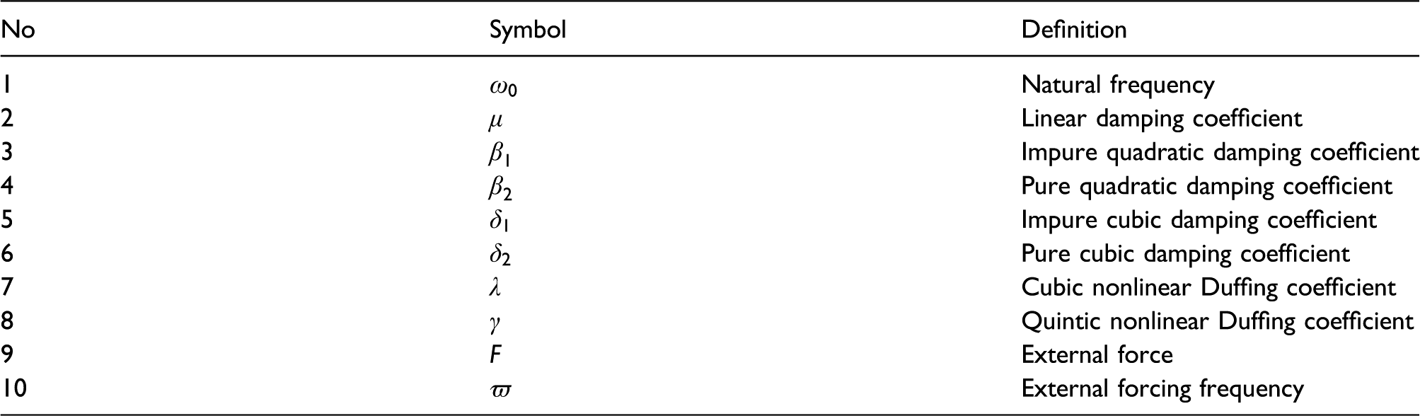
For simplicity, the coefficients that appear in equation (1) may be listed as follows:

No	Symbol	Definition
1	${\omega }_0$	Natural frequency
2	$\mu$	Linear damping coefficient
3	${\beta }_1$	Impure quadratic damping coefficient
4	${\beta }_2$	Pure quadratic damping coefficient
5	${\delta }_1$	Impure cubic damping coefficient
6	${\delta }_2$	Pure cubic damping coefficient
7	$\lambda$	Cubic nonlinear Duffing coefficient
8	$\gamma$	Quintic nonlinear Duffing coefficient
9	$F$	External force
10	$\varpi$	External forcing frequency

Constructed with the aforementioned features, the current study aims to examine the NIPPF controller under an external force as the HRVD oscillator. The vibrating system is calculated analytically by using the frequency response equation. Furthermore, to determine the optimal conditions for the operation of the system, frequency response curves are plotted for different values ​of the controller and system parameters. The validations of time history figures and frequency response curves (FRCs) for the analytical and numerical results are satisfied. To crystallize the presentation of the current work, the rest of the article is structured as follows: Linearized Stability of the HRVD is devoted to adapting the Lindstedt–Poincaré technique in order to extract an analytic bounded solution of the HVPD oscillator. Controller Design via Multiple Scales Method examines the linearized stability of the considered problem. This section involves the phase portraits around the equilibrium points of the HRVD oscillator. The controller design that is proposed by using the multiple scales method and its subsections is introduced in Steady-State Solution. Finally, based on the fundamental findings, the concluding remarks are given throughout Conclusions.

Poincaré–Lindstedt technique

In perturbation theory, the Lindstedt–Poincaré technique (L-P) ²⁷ is a procedure for approximating consistent periodic solutions to differential equations which the classical perturbation approaches fail to provide. In this section, developing the L-P yields the bounded periodic solution of equation (1). In this approach, equation (1) may be written in light of the HPM sense as follows

$$\ddot{x}+{\omega }_0^2\hspace{0.17em}x+\rho \left(2\mu \hspace{0.17em}\dot{x}+{\beta }_1\hspace{0.17em}x\hspace{0.17em}\dot{x}+{\beta }_2{\dot{x}}^2+{\delta }_1\hspace{0.17em}{x}^2\dot{x}+{\delta }_2{\dot{x}}^3+\lambda \hspace{0.17em}{x}^3+\gamma \hspace{0.17em}{x}^5-F\hspace{0.17em}\cos \hspace{0.17em}\varpi t\right)=0;\hspace{1em}\rho \in \left[\mathrm{0,1}\right]$$

(2)

where $\rho$ represents a small embedding homotopy parameter.

Along with the current methodology, the time-independent variable $t$ will be transformed to another time-independent variable $\tau$ like $\tau =\omega t$ , where $\omega$ is defined as an artificial frequency of the given oscillator.

It follows that equation (2) may be transferred to the following equation

$${\omega }^2{x}^{″}+{\omega }_0^2\hspace{0.17em}x+\rho \left(2\mu \hspace{0.17em}\omega \hspace{0.17em}{x}^{\prime }+{\beta }_1\hspace{0.17em}\omega \hspace{0.17em}x\hspace{0.17em}{x}^{\prime }+{\beta }_2\hspace{0.17em}{\omega }^2{x^{\prime }}^2+{\delta }_1\hspace{0.17em}\omega \hspace{0.17em}{x}^2{x}^{\prime }+{\delta }_2{\omega }^3{x^{\prime }}^3+\lambda \hspace{0.17em}{x}^3+\gamma \hspace{0.17em}{x}^5-F\hspace{0.17em}\cos \hspace{0.17em}\varpi \tau -F\rho \hspace{0.17em}{\mathrm{\Omega }}_1\sin \hspace{0.17em}\varpi \tau \right)=0$$

(3)

herein, the prime denotes the differentiation with respect to the independent variable $\tau$ .

In order to obtain acceptable secular terms, the initial conditions (I. C.) may be modified as follows

$$x\left(0\right)={\displaystyle \sum _{j=0}^{\infty }{\rho }^j{a}_j},\hspace{0.17em}\text{and}\hspace{0.17em}\dot{x}\left(0\right)=0$$

(4)

where $a_j,\hspace{1em}j=\mathrm{1,2...}$ are arbitrate constants to be determined later.

According to the methodology of the P-L, the function $x$ and parameter $\omega$ are expanded in powers of $\rho$ as follows

$$x\left(t\right)={\displaystyle \sum _{j=0}^{\infty }{\rho }^j{x}_j\left(t\right)=x_0\left(t\right)+\rho \hspace{0.17em}{x}_1\left(t\right)+{\rho }^2{x}_2\left(t\right)+\mathrm{....}}\text{,}\hspace{0.17em}\text{and,}\hspace{1em}\omega =1+\rho \hspace{0.17em}{\mathrm{\Omega }}_1+{\rho }^2{\mathrm{\Omega }}_2+\mathrm{........}$$

(5)

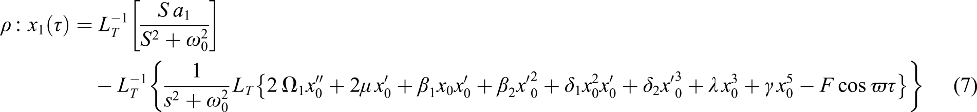
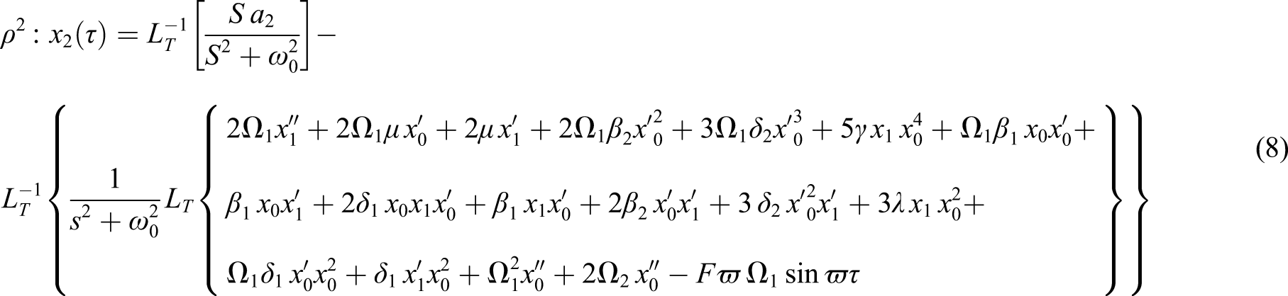
Substituting equations (5) into (3) and identifying the coefficients of the same powers of $\rho$ on both sides, one finds the following hierarchy equations

$${\rho }^0:\hspace{0.17em}{x}_0\left(\tau \right)=a_0\cos \hspace{0.17em}{\omega }_0\tau$$

(6)

where the initial conditions (4) are utilized.

$$\rho :\hspace{0.17em}{x}_1\left(\tau \right)=L_T^{-1}\left[\frac{S\hspace{0.17em}{a}_1}{S^2+{\omega }_0^2}\right]-L_T^{-1}\left\{\frac{1}{s^2+{\omega }_0^2}{L}_T\left\{2\hspace{0.17em}{\mathrm{\Omega }}_1{x}_0^{″}+2\mu \hspace{0.17em}{x}_0^{\prime }+{\beta }_1{x}_0{x}_0^{\prime }+{\beta }_2{x^{\prime }}_0^2+{\delta }_1{x}_0^2{x}_0^{\prime }+{\delta }_2{x^{\prime }}_0^3+\lambda \hspace{0.17em}{x}_0^3+\gamma \hspace{0.17em}{x}_0^5-F\cos \hspace{0.17em}\varpi \tau \right\}\right\}$$

(7)

and

$$\begin{array}{l}{\rho }^2:\hspace{0.17em}{x}_2\left(\tau \right)=L_T^{-1}\left[\frac{S\hspace{0.17em}{a}_2}{S^2+{\omega }_0^2}\right]-\\ L_T^{-1}\left\{\frac{1}{s^2+{\omega }_0^2}{L}_T\left\{\begin{array}{l}2{\mathrm{\Omega }}_1{x}_1^{″}+2{\mathrm{\Omega }}_1\mu \hspace{0.17em}{x}_0^{\prime }+2\mu \hspace{0.17em}{x}_1^{\prime }+2{\mathrm{\Omega }}_1{\beta }_2{x^{\prime }}_0^2+3{\mathrm{\Omega }}_1{\delta }_2{x^{\prime }}_0^3+5\gamma \hspace{0.17em}{x}_1\hspace{0.17em}{x}_0^4+{\mathrm{\Omega }}_1{\beta }_1\hspace{0.17em}{x}_0{x}_0^{\prime }+\\ {\beta }_1\hspace{0.17em}{x}_0{x}_1^{\prime }+2{\delta }_1\hspace{0.17em}{x}_0{x}_1{x}_0^{\prime }+{\beta }_1\hspace{0.17em}{x}_1{x}_0^{\prime }+2{\beta }_2\hspace{0.17em}{x}_0^{\prime }{x}_1^{\prime }+3\hspace{0.17em}{\delta }_2\hspace{0.17em}{x^{\prime }}_0^2{x}_1^{\prime }+3\lambda \hspace{0.17em}{x}_1\hspace{0.17em}{x}_0^2+\\ {\mathrm{\Omega }}_1{\delta }_1\hspace{0.17em}{x}_0^{\prime }{x}_0^2+{\delta }_1\hspace{0.17em}{x}_1^{\prime }{x}_0^2+{\mathrm{\Omega }}_1^2{x}_0^{″}+2{\mathrm{\Omega }}_2\hspace{0.17em}{x}_0^{″}-F\varpi \hspace{0.17em}{\mathrm{\Omega }}_1\sin \hspace{0.17em}\varpi \tau \end{array}\right\}\right\}\end{array}$$

(8)

As identified by equations (7) and (8), the solution of first and second orders depends fundamentally on the zero-order solution.

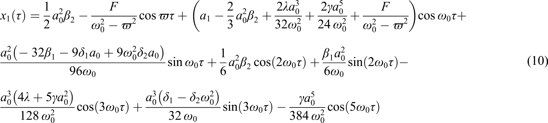
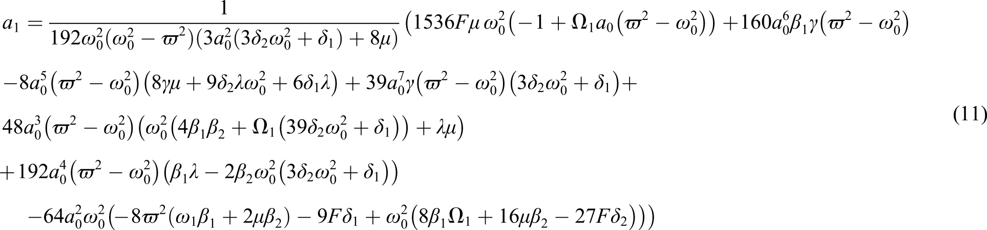
On substituting equations (6) into (7), by using the Mathematica software version 12.2.0.0, the uniform valid expansion requires a cancellation of the substance of the secular terms. Therefore, the coefficients of the functions $\cos \hspace{0.17em}{\omega }_0\tau$ and $\sin \hspace{0.17em}{\omega }_0\tau$ must be canceled. Consequently, the parameters $a_0$ and ${\mathrm{\Omega }}_1$ are determined as follows

$$a_0=2\sqrt{\frac{-2\mu }{{\delta }_1+3{\delta }_2{\omega }_0^2}}\hspace{1em}\text{and,}\hspace{1em}{\mathrm{\Omega }}_1=\frac{\mu \left(20\gamma \hspace{0.17em}\mu -3\lambda \hspace{0.17em}{\delta }_1-9\lambda \hspace{0.17em}{\delta }_2{\omega }_0^2\right)}{{\omega }_0^2{\left({\delta }_1+3{\delta }_2{\omega }_0^2\right)}^2}$$

(9)

It follows that the periodic solution $x_1\left(\tau \right)$ then becomes

$$\begin{array}{l}{x}_1\left(\tau \right)=\frac{1}{2}{a}_0^2{\beta }_2-\frac{F}{{\omega }_0^2-{\varpi }^2}\cos \hspace{0.17em}\varpi \tau +\left(a_1-\frac{2}{3}{a}_0^2{\beta }_2+\frac{2\lambda a_0^3}{32{\omega }_0^2}+\frac{2\gamma a_0^5}{24\hspace{0.17em}{\omega }_0^2}+\frac{F}{{\omega }_0^2-{\varpi }^2}\right)\cos \hspace{0.17em}{\omega }_0\tau +\\ \frac{a_0^2\left(-32{\beta }_1-9{\delta }_1{a}_0+9{\omega }_0^2{\delta }_2{a}_0\right)}{96{\omega }_0}\sin \hspace{0.17em}{\omega }_0\tau +\frac{1}{6}{a}_0^2{\beta }_2\cos \left(2{\omega }_0\tau \right)+\frac{{\beta }_1{a}_0^2}{6{\omega }_0}\sin \left(2{\omega }_0\tau \right)-\\ \frac{a_0^3\left(4\lambda +5\gamma a_0^2\right)}{128\hspace{0.17em}{\omega }_0^2}\cos \left(3{\omega }_0\tau \right)+\frac{a_0^3\left({\delta }_1-{\delta }_2{\omega }_0^2\right)}{32\hspace{0.17em}{\omega }_0}\sin \left(3{\omega }_0\tau \right)-\frac{\gamma a_0^5}{384\hspace{0.17em}{\omega }_0^2}\cos \left(5{\omega }_0\tau \right)\end{array}$$

(10)

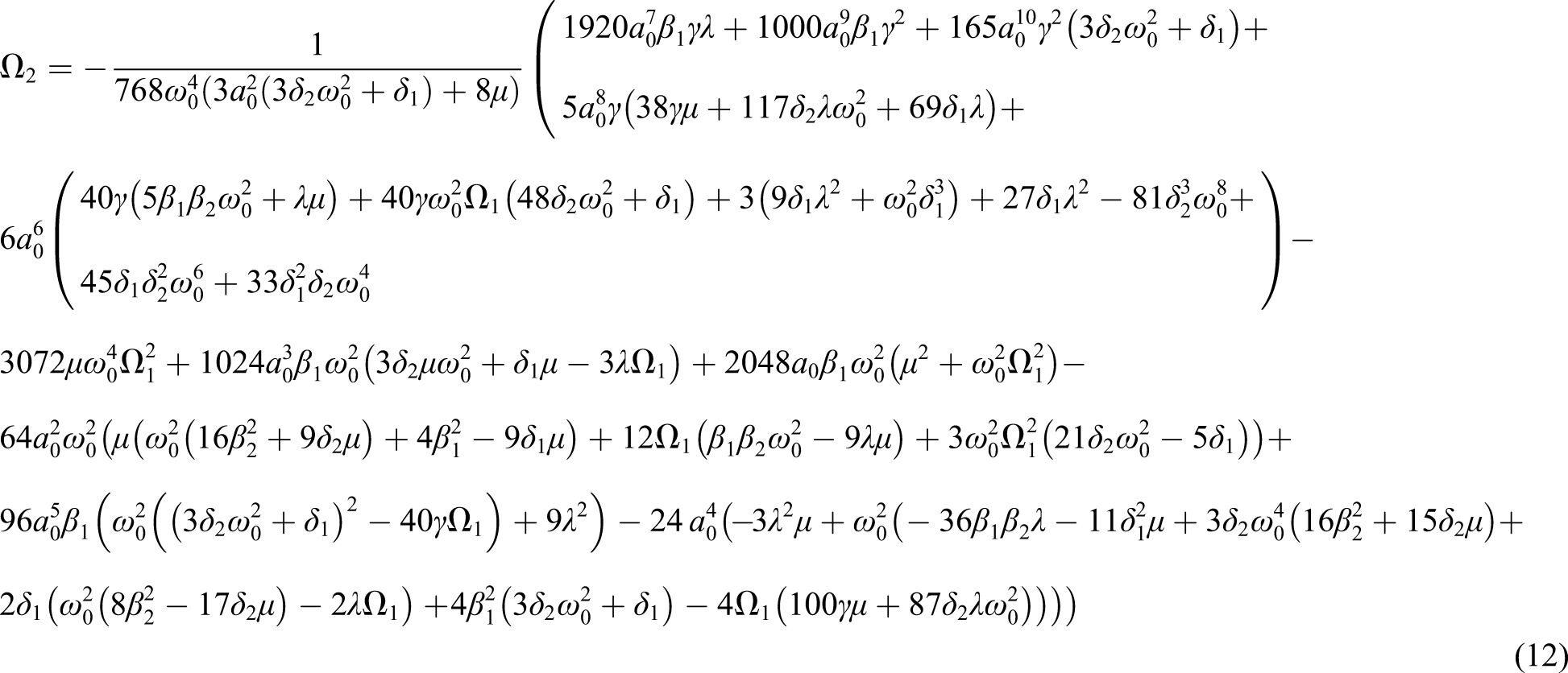
Once more, substituting equations (6), (9), and (10) into (8), the invalidation of the secular terms makes the parameters $a_1$ and ${\mathrm{\Omega }}_2$ to be determined as follows

$$\begin{array}{l}{a}_1=\frac{1}{192{\omega }_0^2\left({\omega }_0^2-{\varpi }^2\right)\left(3a_0^2\left(3{\delta }_2{\omega }_0^2+{\delta }_1\right)+8\mu \right)}(1536F\mu \hspace{0.17em}{\omega }_0^2\left(-1+{\mathrm{\Omega }}_1{a}_0\left({\varpi }^2-{\omega }_0^2\right)\right)+160a_0^6{\beta }_1\gamma \left({\varpi }^2-{\omega }_0^2\right)\\ -8a_0^5\left({\varpi }^2-{\omega }_0^2\right)\left(8\gamma \mu +9{\delta }_2\lambda {\omega }_0^2+6{\delta }_1\lambda \right)+39a_0^7\gamma ({\varpi }^2-{\omega }_0^2)\left(3{\delta }_2{\omega }_0^2+{\delta }_1\right)+\\ 48a_0^3\left({\varpi }^2-{\omega }_0^2\right)\left({\omega }_0^2\left(4{\beta }_1{\beta }_2+{\mathrm{\Omega }}_1\left(39{\delta }_2{\omega }_0^2+{\delta }_1\right)\right)+\lambda \mu \right)\\ +192a_0^4\left({\varpi }^2-{\omega }_0^2\right)\left({\beta }_1\lambda -2{\beta }_2{\omega }_0^2\left(3{\delta }_2{\omega }_0^2+{\delta }_1\right)\right)\\ -64a_0^2{\omega }_0^2\left(-8{\varpi }^2({\omega }_1{\beta }_1+2\mu {\beta }_2)-9F{\delta }_1+{\omega }_0^2(8{\beta }_1{\mathrm{\Omega }}_1+16\mu {\beta }_2-27F{\delta }_2)\right)\end{array}$$

(11)

and

$$\begin{array}{l}{\mathrm{\Omega }}_2=-\frac{1}{768{\omega }_0^4\left(3a_0^2\left(3{\delta }_2{\omega }_0^2+{\delta }_1\right)+8\mu \right)}(\begin{array}{l}1920a_0^7{\beta }_1\gamma \lambda +1000a_0^9{\beta }_1{\gamma }^2+165a_0^{10}{\gamma }^2\left(3{\delta }_2{\omega }_0^2+{\delta }_1\right)+\\ 5a_0^8\gamma \left(38\gamma \mu +117{\delta }_2\lambda {\omega }_0^2+69{\delta }_1\lambda \right)+\end{array}\\ 6a_0^6\left(\begin{array}{l}40\gamma \left(5{\beta }_1{\beta }_2{\omega }_0^2+\lambda \mu \right)+40\gamma {\omega }_0^2{\mathrm{\Omega }}_1\left(48{\delta }_2{\omega }_0^2+{\delta }_1\right)+3\left(9{\delta }_1{\lambda }^2+{\omega }_0^2{\delta }_1^3\right)+27{\delta }_1{\lambda }^2-81{\delta }_2^3{\omega }_0^8+\\ 45{\delta }_1{\delta }_2^2{\omega }_0^6+33{\delta }_1^2{\delta }_2{\omega }_0^4\end{array}\right)-\\ 3072\mu {\omega }_0^4{\mathrm{\Omega }}_1^2+1024a_0^3{\beta }_1{\omega }_0^2\left(3{\delta }_2\mu {\omega }_0^2+{\delta }_1\mu -3\lambda {\mathrm{\Omega }}_1\right)+2048a_0{\beta }_1{\omega }_0^2\left({\mu }^2+{\omega }_0^2{\mathrm{\Omega }}_1^2\right)-\\ 64a_0^2{\omega }_0^2\left(\mu \left({\omega }_0^2\left(16{\beta }_2^2+9{\delta }_2\mu \right)+4{\beta }_1^2-9{\delta }_1\mu \right)+12{\mathrm{\Omega }}_1\left({\beta }_1{\beta }_2{\omega }_0^2-9\lambda \mu \right)+3{\omega }_0^2{\mathrm{\Omega }}_1^2\left(21{\delta }_2{\omega }_0^2-5{\delta }_1\right)\right)+\\ 96a_0^5{\beta }_1\left({\omega }_0^2\left({\left(3{\delta }_2{\omega }_0^2+{\delta }_1\right)}^2-40\gamma {\mathrm{\Omega }}_1\right)+9{\lambda }^2\right)-24\hspace{0.17em}{a}_0^4(-3{\lambda }^2\mu +{\omega }_0^2(-36{\beta }_1{\beta }_2\lambda -11{\delta }_1^2\mu +3{\delta }_2{\omega }_0^4\left(16{\beta }_2^2+15{\delta }_2\mu \right)+\\ 2{\delta }_1\left({\omega }_0^2\left(8{\beta }_2^2-17{\delta }_2\mu \right)-2\lambda {\mathrm{\Omega }}_1\right)+4{\beta }_1^2\left(3{\delta }_2{\omega }_0^2+{\delta }_1\right)-4{\mathrm{\Omega }}_1\left(100\gamma \mu +87{\delta }_2\lambda {\omega }_0^2\right))))\end{array}$$

(12)

It follows that the uniform valid solution $x_2\left(\tau \right)$ becomes

$$\begin{array}{l}{x}_2\left(\tau \right)=A_0+A_1\cos \hspace{0.17em}{\omega }_0\tau +A_2\hspace{0.17em}\sin \hspace{0.17em}{\omega }_0\tau +A_3\cos \left(2{\omega }_0\tau \right)+A_4\sin \left(2{\omega }_0\tau \right)+A_5\cos \left(3{\omega }_0\tau \right)+A_6\sin \left(3{\omega }_0\tau \right)+\\ A_7\cos \left(4{\omega }_0\tau \right)+A_8\sin \left(4{\omega }_0\tau \right)+A_9\cos \left(5{\omega }_0\tau \right)+A_{10}\sin \left(5{\omega }_0\tau \right)+A_{11}\cos \left(6{\omega }_0\tau \right)+A_{12}\sin \left(6{\omega }_0\tau \right)+\\ A_{13}\cos \left(7{\omega }_0\tau \right)+A_{14}\sin \left(7{\omega }_0\tau \right)+A_{15}\cos \left(9{\omega }_0\tau \right)+A_{16}\cos \left(\varpi \tau \right)+A_{17}\sin \left(\varpi \tau \right)+A_{18}\cos \left(\varpi +{\omega }_0\right)\tau +\\ A_{19}\sin \left(\varpi +{\omega }_0\right)\tau +A_{20}\cos \left(\varpi -{\omega }_0\right)\tau +A_{21}\sin \left(\varpi -{\omega }_0\right)\tau +A_{22}\cos \left(\varpi +2{\omega }_0\right)\tau +A_{23}\sin \left(\varpi +2{\omega }_0\right)\tau \\ A_{24}\cos \left(\varpi -2{\omega }_0\right)\tau +A_{25}\sin \left(\varpi -2{\omega }_0\right)\tau +A_{26}\cos \left(\varpi +4{\omega }_0\right)\tau +A_{27}\cos \left(\varpi -4{\omega }_0\right)\tau \end{array}$$

(13)

where the constants $A_i$ , $i=1,2,...,27$ . In order to follow the study more easily, they will be moved from the study.To obtain the constant $a_2$ , we need to eliminate the secular terms of the third-order solution. This procedure is very tedious, yet straightforward. For easier follow-up of the study, it will be removed.

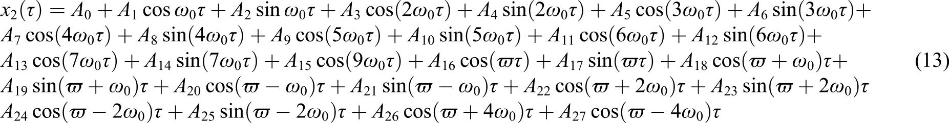
Finally, the approximate bounded solution of the equation of motion that is given in equation (1) will be written as follows

$$x\left(\tau \right)=\underset{\rho \to 1}{\lim }\left(x_0\left(\tau \right)+\rho \hspace{0.17em}{x}_1\left(\tau \right)+{\rho }^2{x}_2\left(\tau \right)\right)$$

(14)

where $x_0\left(\tau \right),x_1\left(\tau \right)$ , and $x_2\left(\tau \right)$ are the time-dependent functions that are given by equations (6), (10), and (13), respectively.

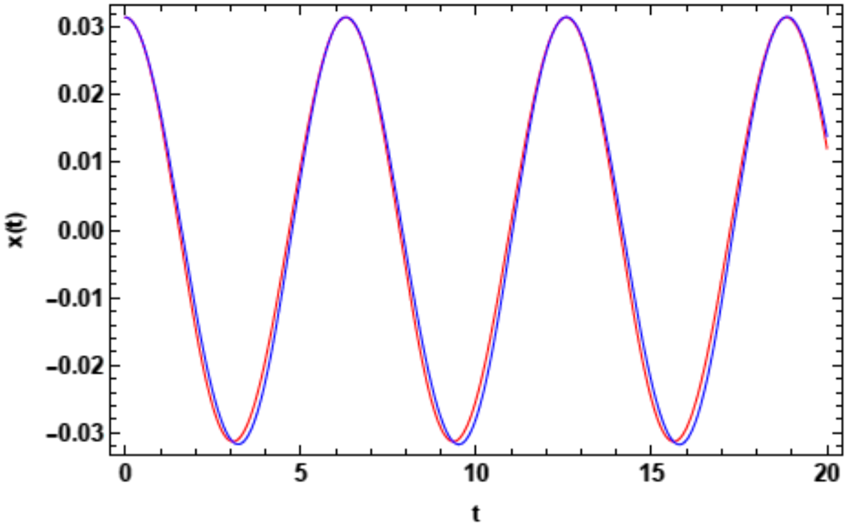
To check the feasibility of the implication of the previous L-P, it is appropriate to compare this method with the numerical methodology known as RK4. Therefore, in what follows the analytic approximate solution as given by equation (14) is sketched in red. On the other hand, the RK4 of the considered system as given by equation (1) is plotted in blue. The following figure is graphed of a system having the following particulars:

$${\omega }_0=1,\hspace{0.17em}\mu =-0.0005,\hspace{0.17em}{\beta }_1=3.5,\hspace{0.17em}{\beta }_2=0.125,\hspace{0.17em}{\delta }_1=1.05,\hspace{0.17em}{\delta }_2=0.85,\lambda =-0.6,\hspace{0.17em}\gamma =0.05,\hspace{0.17em}F=0.5\hspace{0.17em}\text{and}\hspace{0.17em}\varpi =200$$

According to these particulars, the first initial condition then becomes: $x\left(0\right)=0.0\hspace{0.17em}3147$ . This value is very essential as an initial condition for the implication of the software RK4.

As shown from this figure, the two curves are nearly coincident. This shows that L-P, as an analytic approximate solution, is a promising and powerful perturbed technique Figures 1–7.

Figure 1.

Perturbed solution as given in equation (14).

Figure 2.

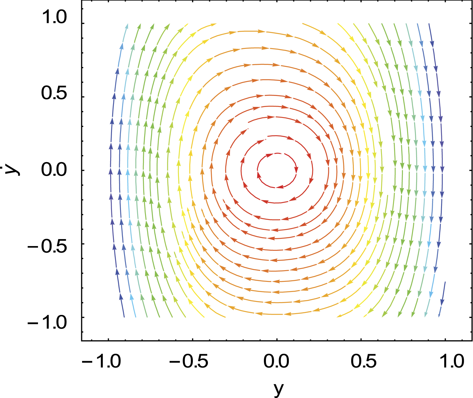
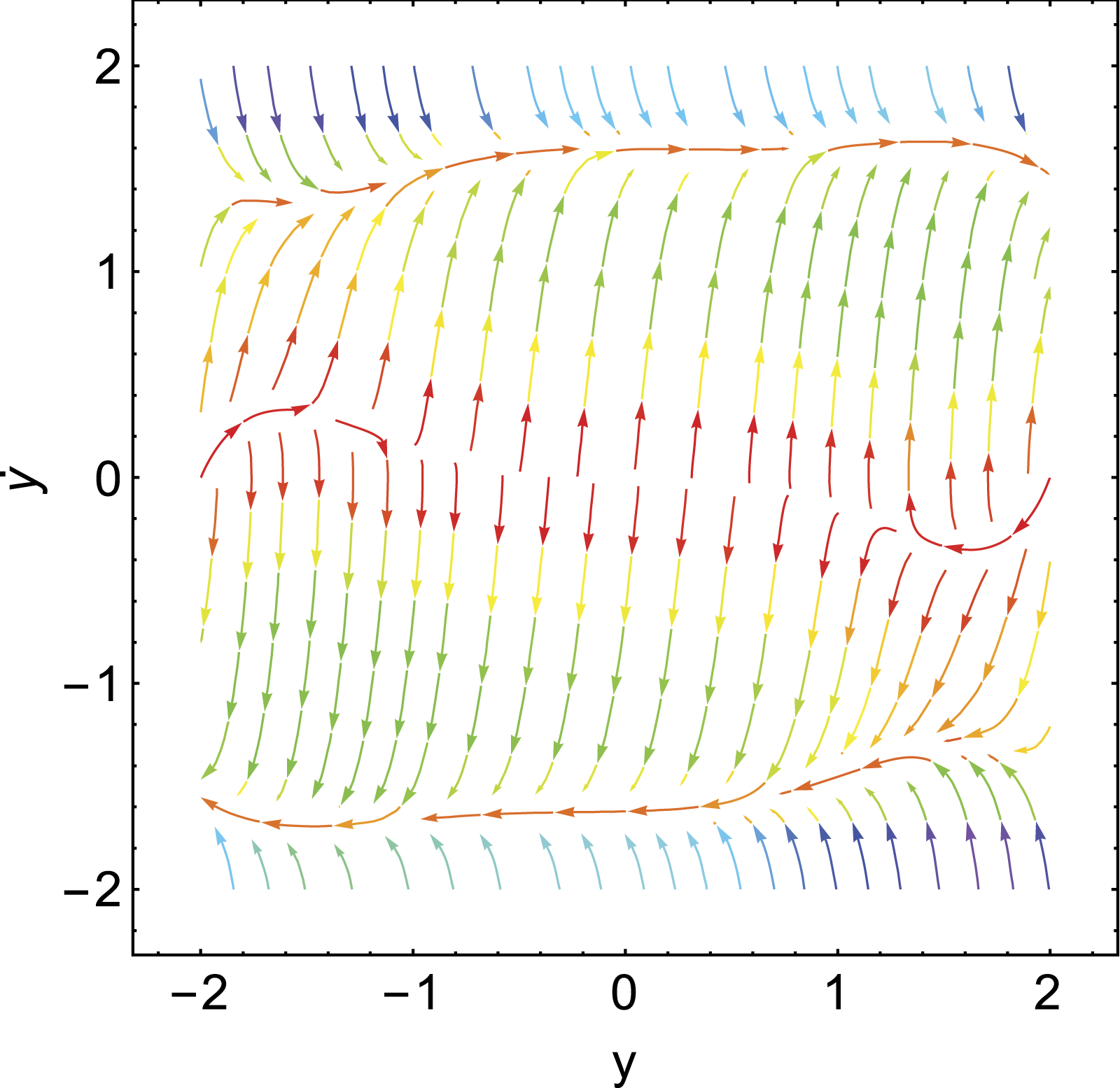
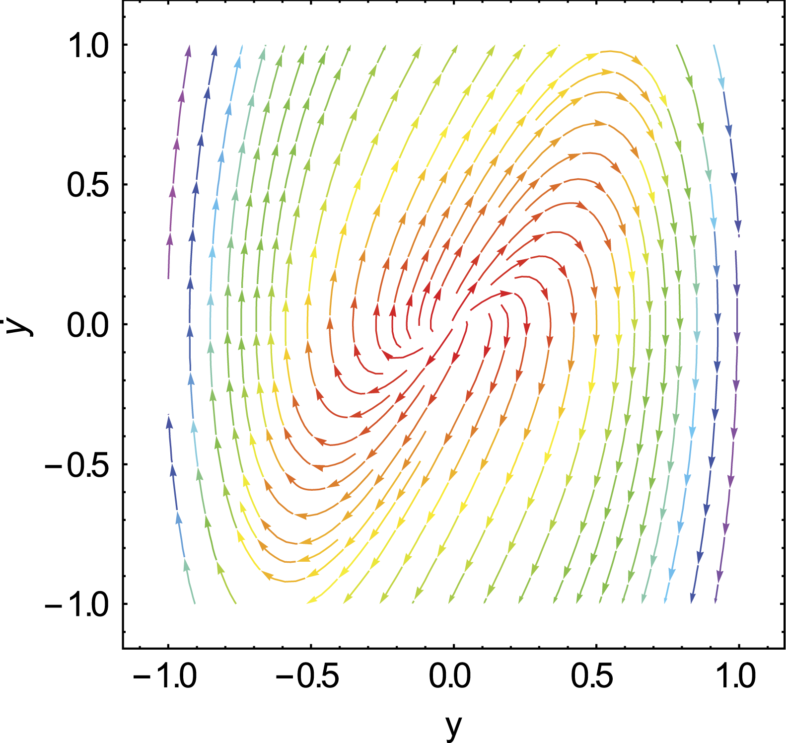
Dynamical behavior (stable center) with given parameters listed in Table 1.

Figure 3.

Dynamical behavior (unstable saddle point) with given parameters listed in Table 1.

Figure 4.

Dynamical behavior (unstable saddle point) with given parameters listed in Table 1.

Figure 5.

Dynamical behavior (unstable saddle point) with given parameters listed in Table 1.

Figure 6.

Dynamical behavior (unstable saddle point) with given parameters listed in Table 1.

Figure 7.

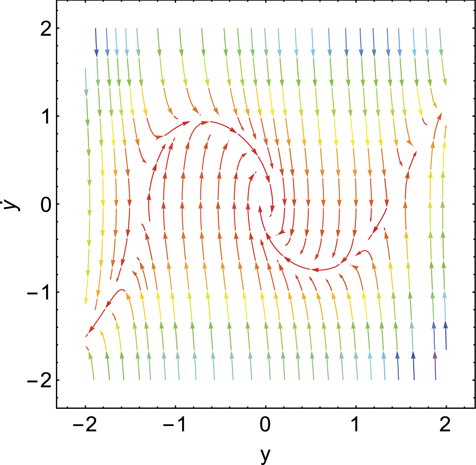
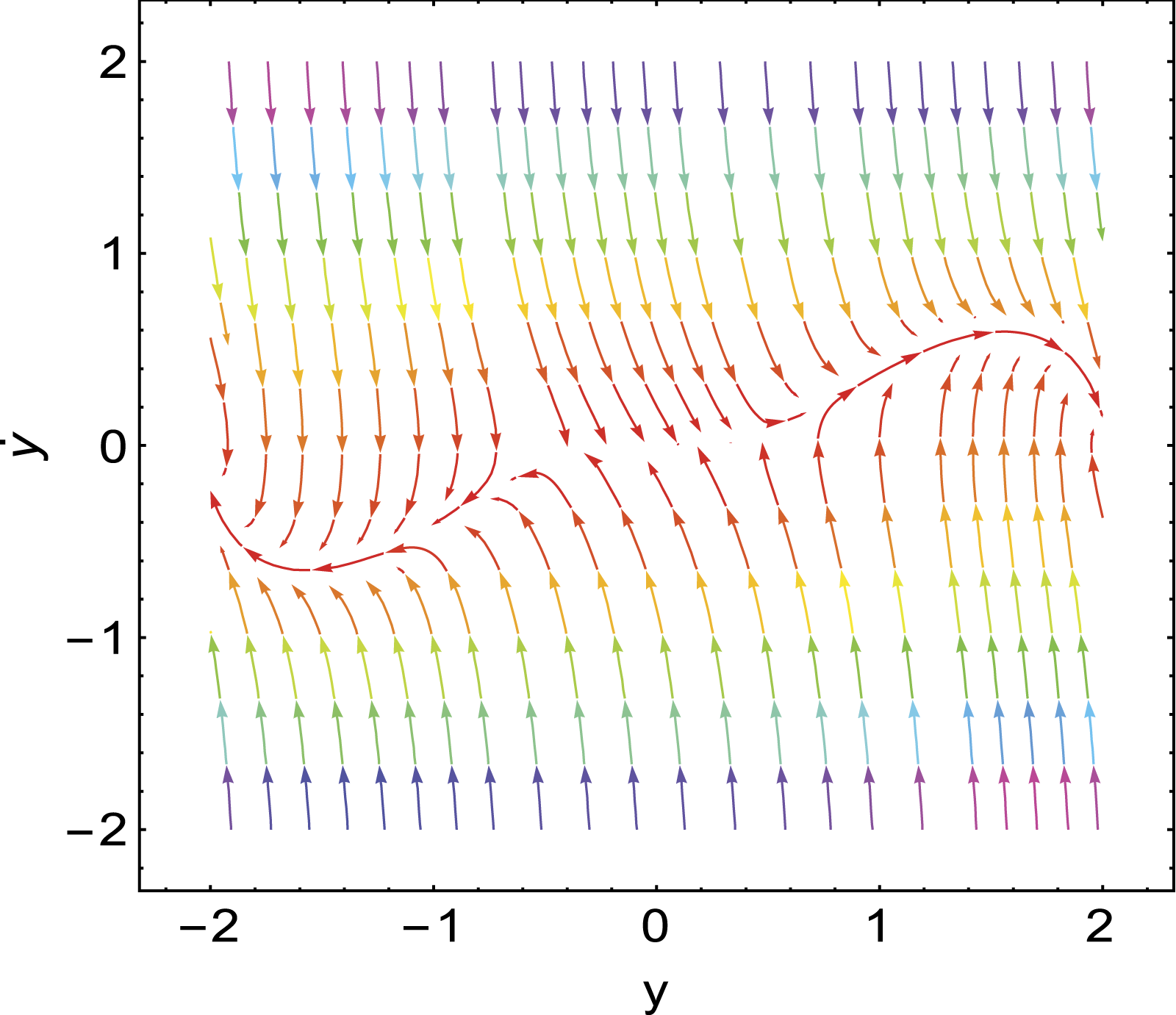
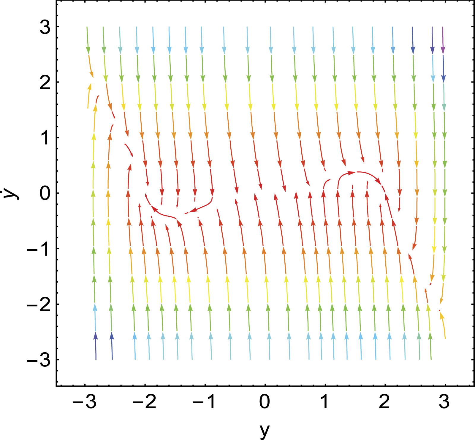
Dynamical behavior (unstable saddle point) with given parameters listed in Table 1.

Linearized Stability of the HRVD

Throughout this section, the linearized technique is employed for the HRVD as given by equation (1). Unfortunately, the following procedure is valid only for the autonomous system. Therefore, an external force must be neglected, or $F\to 0$ .

Along with this approach, the autonomous system of the HRVD then becomes

$$\ddot{x}+{\omega }_0^2\hspace{0.17em}x+2\mu \hspace{0.17em}\dot{x}+{\beta }_1\hspace{0.17em}x\hspace{0.17em}\dot{x}+{\beta }_2{\dot{x}}^2+{\delta }_1\hspace{0.17em}{x}^2\dot{x}+{\delta }_2{\dot{x}}^3+\lambda \hspace{0.17em}{x}^3+\gamma \hspace{0.17em}{x}^5=0$$

(15)

Considering the transformation: $\dot{x}=y$ , it follows that equation (15) may be converted to the following system

$$\dot{x}=g\left(x,y\right),\dot{y}=h\left(x,y\right)$$

(16)

where

$$g\left(x,y\right)=y,h\left(x,y\right)=-{\omega }_0^2\hspace{0.17em}x-2\mu \hspace{0.17em}\dot{x}-{\beta }_1\hspace{0.17em}x\hspace{0.17em}\dot{x}-{\beta }_2{\dot{x}}^2-{\delta }_1\hspace{0.17em}{x}^2\dot{x}-{\delta }_2{\dot{x}}^3-\lambda \hspace{0.17em}{x}^3-\gamma \hspace{0.17em}{x}^5$$

(17)

The fixed points (equilibrium points) happen at the points $\left(x_0,y_0\right)$ , where

$$g\left(x_0,y_0\right)=0,h\left(x_0,y_0\right)=0$$

(18)

It follows that

$$y_0=0$$

(19)

and

$${\omega }_0^2\hspace{0.17em}{x}_0+2\mu \hspace{0.17em}{y}_0+{\beta }_1\hspace{0.17em}{x}_0\hspace{0.17em}{y}_0+{\beta }_2{y}_0^2+{\delta }_1\hspace{0.17em}{x}_0^2{y}_0+{\delta }_2{y}_0^3+\lambda \hspace{0.17em}{x}_0^3+\gamma \hspace{0.17em}{x}_0^5=0$$

(20)

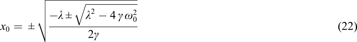
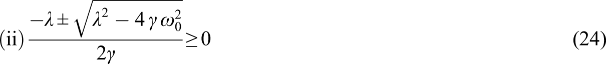
It follows that there are five fixed points as follows

$$y_0=0$$

(21)

and

$$x_0=\pm \sqrt{\frac{-\lambda \pm \sqrt{{\lambda }^2-4\hspace{0.17em}\gamma \hspace{0.17em}{\omega }_0^2}}{2\gamma }}$$

(22)

In order to obtain real equilibrium points, the following conditions must be satisfied

$$\left(\text{i}\right){\lambda }^2\ge 4\hspace{0.17em}\gamma \hspace{0.17em}{\omega }_0^2$$

(23)

and

$$\left(\text{ii}\right)\hspace{0.17em}\frac{-\lambda \pm \sqrt{{\lambda }^2-4\hspace{0.17em}\gamma \hspace{0.17em}{\omega }_0^2}}{2\gamma }\ge 0$$

(24)

Expanding the Taylor expansion up to the first order to develop the functions $g\left(x,y\right)$ and $h\left(x,y\right)$ round the critical points, one finds the following Jacobian matrix

$$J=\left(\begin{array}{cc}0& 1\\ -\left({\omega }_0^2+{\beta }_1\hspace{0.17em}{y}_0+2{\delta }_1\hspace{0.17em}{x}_0{y}_0+3\lambda \hspace{0.17em}{x}_0^2+5\gamma \hspace{0.17em}{x}_0^4\right)& -\left(2\mu +{\beta }_1\hspace{0.17em}{x}_0+2{\beta }_2{y}_0+{\delta }_1\hspace{0.17em}{x}_0^2+3{\delta }_2{y}_0^2\right)\end{array}\right)$$

(25)

It follows that at the equilibrium points, the Jacobian matrix becomes

$$J=\left(\begin{array}{cc}-\mathrm{\Lambda }& 1\\ -\left({\omega }_0^2+{\beta }_1\hspace{0.17em}{y}_0+2{\delta }_1\hspace{0.17em}{x}_0{y}_0+3\lambda \hspace{0.17em}{x}_0^2+5\gamma \hspace{0.17em}{x}_0^4\right)& -\left(2\mu +{\beta }_1\hspace{0.17em}{x}_0+2{\beta }_2{y}_0+{\delta }_1\hspace{0.17em}{x}_0^2+3{\delta }_2{y}_0^2\right)-\mathrm{\Lambda }\end{array}\right)$$

(26)

From the above matrix, the eigenvalues are given as

$${\mathrm{\Lambda }}_{\mathrm{1,2}}=\frac{-1}{2}\left(2\mu +{\beta }_1{x}_0+2{\beta }_2{y}_0+{\delta }_1{x}_0^2+3{\delta }_2{y}_0^2\pm \sqrt{\begin{array}{l}{\left(2\mu +{\beta }_1\hspace{0.17em}{x}_0+2{\beta }_2{y}_0+{\delta }_1\hspace{0.17em}{x}_0^2+3{\delta }_2{y}_0^2\right)}^2\\ -4\left({\omega }_0^2+{\beta }_1\hspace{0.17em}{y}_0+2{\delta }_1\hspace{0.17em}{x}_0{y}_0+3\lambda \hspace{0.17em}{x}_0^2+5\gamma \hspace{0.17em}{x}_0^4\right)\end{array}}\right).$$

(27)

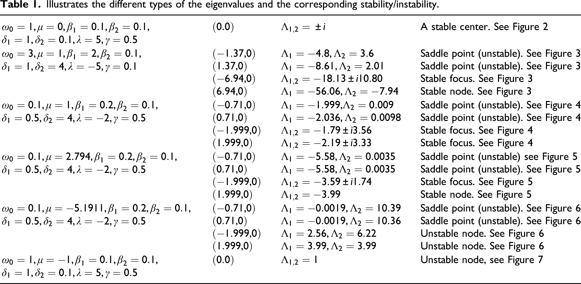
Characteristically, if the eigenvalue of the Jacobian, which is calculated at the equilibrium point, has a negative real part, the equilibrium point becomes a stable state. The equilibrium point, on the other hand, is unstable if at least one of the eigenvalues has a positive real part. It is more appropriate to consider a sample chosen system to indicate the stability/instability configuration in light of the equilibrium points. Consequently, the nature of the eigenvalues gives the criterion. This procedure may be done in the following Table 1.

Table 1.

Illustrates the different types of the eigenvalues and the corresponding stability/instability.

$\begin{array}{l}{\omega }_0=1,\hspace{0.17em}\mu =0,\hspace{0.17em}{\beta }_1=0.1,\hspace{0.17em}{\beta }_2=0.1,\\ {\delta }_1=1,\hspace{0.17em}{\delta }_2=0.1,\hspace{0.17em}\lambda =5,\hspace{0.17em}\gamma =0.5\end{array}$	$\left(0.0\right)$	${\mathrm{\Lambda }}_{\mathrm{1,2}}=\pm i$	A stable center. See Figure 2
$\begin{array}{l}{\omega }_0=3,\hspace{0.17em}\mu =1,\hspace{0.17em}{\beta }_1=2,\hspace{0.17em}{\beta }_2=0.1,\\ {\delta }_1=1,\hspace{0.17em}{\delta }_2=4,\hspace{0.17em}\lambda =-5,\hspace{0.17em}\gamma =0.1\end{array}$	$\left(-1.37,0\right)$	${\mathrm{\Lambda }}_1=-4.8,\hspace{0.17em}{\mathrm{\Lambda }}_2=3.6$	Saddle point (unstable). See Figure 3
	$\left(1.37,0\right)$	${\mathrm{\Lambda }}_1=-8.61,\hspace{0.17em}{\mathrm{\Lambda }}_2=2.01$	Saddle point (unstable). See Figure 3
	$\left(-6.94,0\right)$	${\mathrm{\Lambda }}_{\mathrm{1,2}}=-18.13\pm i10.80$	Stable focus. See Figure 3
	$\left(6.94,0\right)$	${\mathrm{\Lambda }}_1=-56.06,\hspace{0.17em}{\mathrm{\Lambda }}_2=-7.94$	Stable node. See Figure 3
$\begin{array}{l}{\omega }_0=0.1,\hspace{0.17em}\mu =1,\hspace{0.17em}{\beta }_1=0.2,\hspace{0.17em}{\beta }_2=0.1,\\ {\delta }_1=0.5,\hspace{0.17em}{\delta }_2=4,\hspace{0.17em}\lambda =-2,\hspace{0.17em}\gamma =0.5\end{array}$	$\left(-0.71,0\right)$	${\mathrm{\Lambda }}_1=-1.999,{\mathrm{\Lambda }}_2=0.009$	Saddle point (unstable). See Figure 4
	$\left(0.71,0\right)$	${\mathrm{\Lambda }}_1=-2.036,\hspace{0.17em}{\mathrm{\Lambda }}_2=0.0098$	Saddle point (unstable). See Figure 4
	$\left(-1.999,0\right)$	${\mathrm{\Lambda }}_{\mathrm{1,2}}=-1.79\pm i3.56$	Stable focus. See Figure 4
	$\left(1.999,0\right)$	${\mathrm{\Lambda }}_{\mathrm{1,2}}=-2.19\pm i3.33$	Stable focus. See Figure 4
$\begin{array}{l}{\omega }_0=0.1,\hspace{0.17em}\mu =2.794,\hspace{0.17em}{\beta }_1=0.2,\hspace{0.17em}{\beta }_2=0.1,\\ {\delta }_1=0.5,\hspace{0.17em}{\delta }_2=4,\hspace{0.17em}\lambda =-2,\hspace{0.17em}\gamma =0.5\end{array}$	$\left(-0.71,0\right)$	${\mathrm{\Lambda }}_1=-5.58,\hspace{0.17em}{\mathrm{\Lambda }}_2=0.0035$	Saddle point (unstable) see Figure 5
	$\left(0.71,0\right)$	${\mathrm{\Lambda }}_1=-5.58,\hspace{0.17em}{\mathrm{\Lambda }}_2=0.0035$	Saddle point (unstable). See Figure 5
	$\left(-1.999,0\right)$	${\mathrm{\Lambda }}_{\mathrm{1,2}}=-3.59\pm i1.74$	Stable focus. See Figure 5
	$\left(1.999,0\right)$	${\mathrm{\Lambda }}_{\mathrm{1,2}}=-3.99$	Stable node. See Figure 5
$\begin{array}{l}{\omega }_0=0.1,\hspace{0.17em}\mu =-5.1911,\hspace{0.17em}{\beta }_1=0.2,\hspace{0.17em}{\beta }_2=0.1,\\ {\delta }_1=0.5,\hspace{0.17em}{\delta }_2=4,\hspace{0.17em}\lambda =-2,\hspace{0.17em}\gamma =0.5\end{array}$	$\left(-0.71,0\right)$	${\mathrm{\Lambda }}_1=-0.0019,\hspace{0.17em}{\mathrm{\Lambda }}_2=10.39$	Saddle point (unstable). See Figure 6
	$\left(0.71,0\right)$	${\mathrm{\Lambda }}_1=-0.0019,\hspace{0.17em}{\mathrm{\Lambda }}_2=10.36$	Saddle point (unstable). See Figure 6
	$\left(-1.999,0\right)$	${\mathrm{\Lambda }}_1=2.56,\hspace{0.17em}{\mathrm{\Lambda }}_2=6.22$	Unstable node. See Figure 6
	$\left(1.999,0\right)$	${\mathrm{\Lambda }}_1=3.99,\hspace{0.17em}{\mathrm{\Lambda }}_2=3.99$	Unstable node. See Figure 6
$\begin{array}{l}{\omega }_0=1,\hspace{0.17em}\mu =-1,\hspace{0.17em}{\beta }_1=0.1,\hspace{0.17em}{\beta }_2=0.1,\\ {\delta }_1=1,\hspace{0.17em}{\delta }_2=0.1,\hspace{0.17em}\lambda =5,\hspace{0.17em}\gamma =0.5\end{array}$	$\left(0.0\right)$	${\mathrm{\Lambda }}_{\mathrm{1,2}}=1$	Unstable node, see Figure 7

Controller Design via Multiple Scales Method

After adding the NIPPF controller, the equation of HRVD subjected to an external force as shown in Miwadinou et al. ³⁵ may be presented as follows

$$\ddot{x}+{\omega }_0^2\hspace{0.17em}x+2\hspace{0.17em}\mu \hspace{0.17em}\dot{x}+{\beta }_1\hspace{0.17em}x\hspace{0.17em}\dot{x}+{\beta }_2{\dot{x}}^2+{\delta }_1\hspace{0.17em}{x}^2\dot{x}+{\delta }_2{\dot{x}}^3+\lambda \hspace{0.17em}{x}^3+\hspace{0.17em}\gamma \hspace{0.17em}{x}^5=F\cos \hspace{0.17em}\omega t+{\alpha }_1\hspace{0.17em}y+{\alpha }_2\hspace{0.17em}z$$

(28)

$$\ddot{y}+{\omega }_1^2\hspace{0.17em}y+2\hspace{0.17em}{\mu }_1\hspace{0.17em}\dot{y}={\gamma }_1\hspace{0.17em}x$$

(29)

and

$$\dot{z}+\rho \hspace{0.17em}z={\gamma }_2\hspace{0.17em}x$$

(30)

As shown by Saeed and Kamel, ⁴¹ the previous coefficients may be chosen as follows

$$\mu ={\epsilon }^2\tilde{\mu },\hspace{0.17em}{\mu }_1={\epsilon }^2{\tilde{\mu }}_1,\hspace{0.17em}F={\epsilon }^2\tilde{F},\hspace{0.17em}{\alpha }_1={\epsilon }^2\hspace{0.17em}{\tilde{\alpha }}_1,\hspace{0.17em}{\alpha }_2={\epsilon }^2\hspace{0.17em}{\tilde{\alpha }}_2,\hspace{0.17em}{\gamma }_1={\epsilon }^2\hspace{0.17em}{\tilde{\gamma }}_1\hspace{0.17em}\text{and}\hspace{0.17em}\gamma ={\epsilon }^{-2}\tilde{\gamma }$$

Along with Amer et al. ³⁸ and Omidi and Mahmoodi, ³⁹ the NIPPF controller can be represented by using three degrees of freedom as shown in equations (33)–(35). It is worthy to notice that the NIPPF controller includes both types of controllers, PPF and IRC. As seen, PPF controller is represented by equation (34) in such a way that ${\gamma }_1$ is PPF gain and ${\alpha }_1$ , which is given in equation (33), is the feedback gain. Additionally, the IRC controller is represented by equation (35) in such a way that ${\gamma }_2$ is the IRC gain, and ${\alpha }_2$ sited in equation (33) is the feedback gain. The displacement of the HRVD is $x$ ; meanwhile, $y$ and $z$ are the displacements of the controllers, ${\mu }_1$ is the linear damping coefficient, ${\omega }_1$ is the natural frequency of the controller, and $\rho$ is the linear parameter.

Now, RK4 is applied to get the numerical results of the time history and phase portraits of HRVD. In what follows, a sample chosen system of particulars is given by the following parameters

$$F=0.965,\hspace{0.17em}{\omega }_0=1,\hspace{0.17em}{\beta }_1=0.5,\hspace{0.17em}{\beta }_2=0.125,\hspace{0.17em}\mu =-0.0005,\hspace{0.17em}{\delta }_1=1.05,\hspace{0.17em}{\delta }_2=0.85,\hspace{0.17em}\lambda =0.6,\hspace{0.17em}\gamma =0.05$$

The following analysis considers the primary resonance case at which $\left(\omega ={\omega }_0\right)$ and the controller parameters are

$${\alpha }_1=0.2,\hspace{0.17em}{\alpha }_2=0.5,\hspace{0.17em}{\alpha }_1=0.2,\hspace{0.17em}{\gamma }_1=0.5,\hspace{0.17em}{\gamma }_2=0.5,\hspace{0.17em}{\mu }_1=0.0005,\hspace{0.17em}\rho ={\omega }_0\hspace{0.17em}\text{at}\hspace{0.17em}{\omega }_1={\omega }_0$$

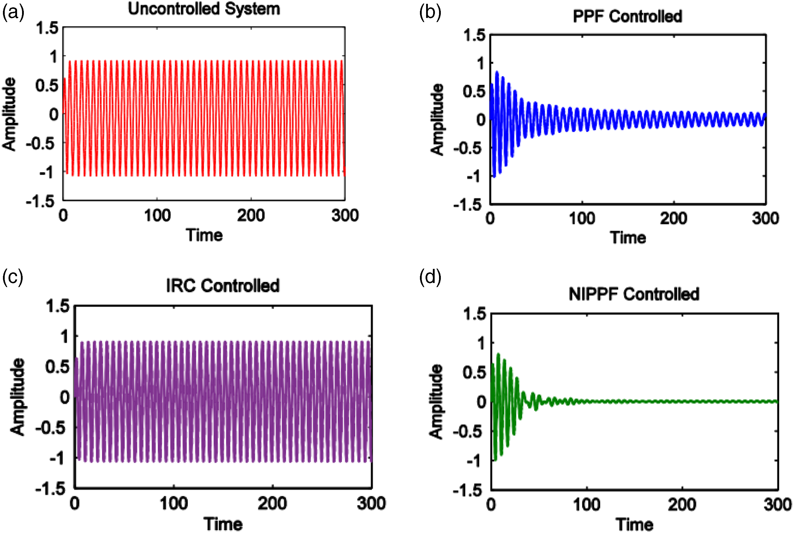
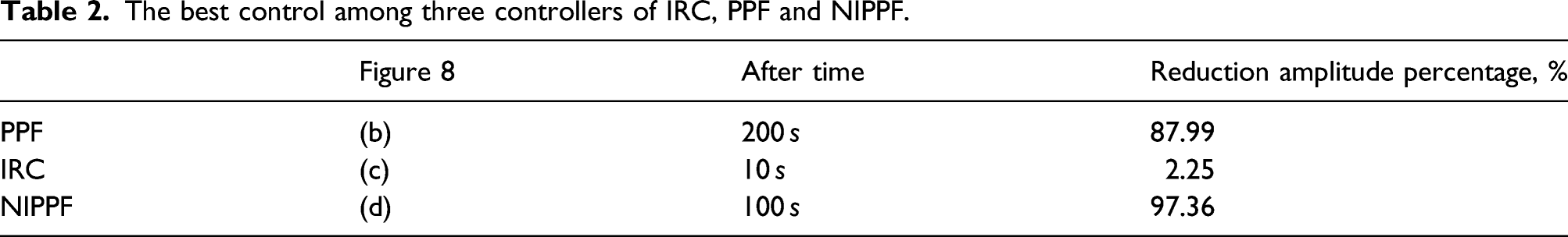
To show the best control between the three controllers IRC, PPF, and NIPPF, the time history of the amplitude is shown in Figure 8. The suppression of the amplitude from its maximum value that is given in Figure 8(a) may be illustrated in the following Table 2

Figure 8.

Time History of the main system when: (a) uncontrolled system, (b) position feedback controller controlled, (c) integral resonant controller controlled, and (d) nonlinear integrated positive position feedback controlled at $\omega ={\omega }_0$ and ${\omega }_1={\omega }_0$ .

Table 2.

The best control among three controllers of IRC, PPF and NIPPF.

	Figure 8	After time	Reduction amplitude percentage, %
PPF	(b)	$200\hspace{0.17em}s$	87.99
IRC	(c)	$10\hspace{0.17em}s$	2.25
NIPPF	(d)	$100\hspace{0.17em}s$	97.36

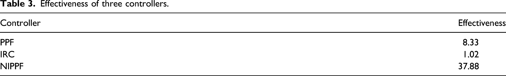
On the other hand, the effectiveness of the previous controllers may be given in Table 2. Remember that the effectiveness ratio $E_a$ is calculated as: $E_a$ (= steady-state amplitude of the system before and divided by after controlling). By using Figure 8(a)–(d), the effectiveness of the various controllers may be listed as in Table 3.

Table 3.

Effectiveness of three controllers.

Controller	Effectiveness
PPF	8.33
IRC	1.02
NIPPF	37.88

This indicates that the effectiveness of the controller NIPPF is the maximum one. Therefore, from Tables 2 and 3, one can say that NIPPF is the best controller to suppress the vibration. Additionally, NIPPF takes a relatively short time to reduce the chaos when compared to both PPF and IRC.

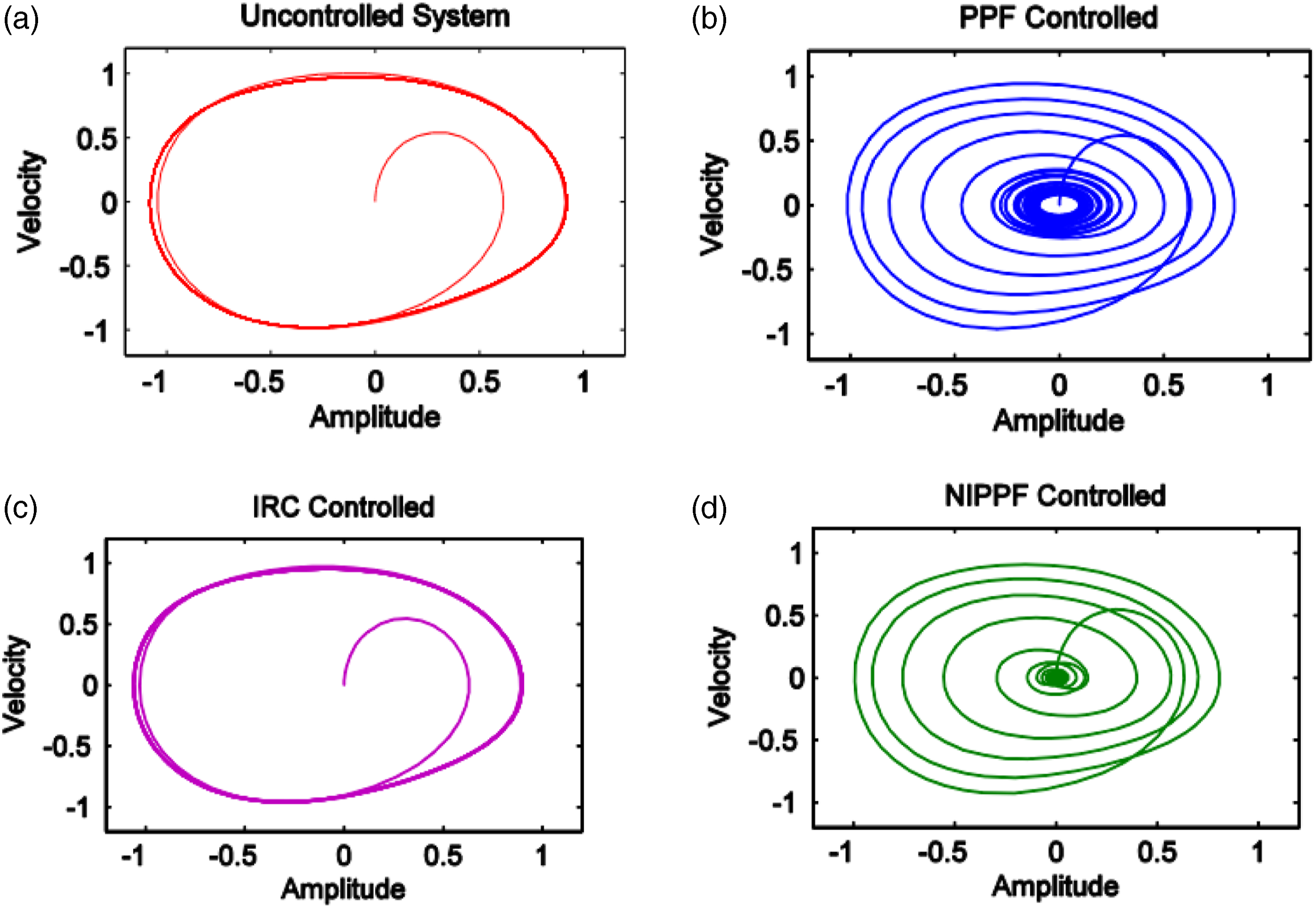
The phase portraits for the main equation and the controllers are plotted in Figure 9. As seen from these figures, the velocity is pictured versus the amplitude. From Figure 9(a) and (c), it is clear that there is a little change between them. By contrast, as in Figure 9(b) and (c), there exists some uniform behavior away from Figure 9(a). Actually, Figure 9(d) gives the finest behavior. Again, this indicates that NIPPF controller is the optimal controller. The obtained results for the time history and phase portrait are in a good agreement with the previous works of Amer et al., ³⁸ Omidi and Mahmoodi, ³⁹ and El-Sayed and Bauomy. ⁴²

Figure 9.

Phase portrait of the main system when: (a) uncontrolled system, (b) position feedback controller controlled, (c) integral resonant controller controlled, and (d) nonlinear integrated positive position feedback controlled at $\omega ={\omega }_0$ and ${\omega }_1={\omega }_0$ .

Returning again to the multiple scales method, ²⁷ along with this approach, one gets the following expansions

$$x\left(t;\epsilon \right)=\epsilon \hspace{0.17em}{x}_1\left(T_0,T_1,T_2\right)+{\epsilon }^2\hspace{0.17em}{x}_2\left(T_0,T_1,T_2\right)+{\epsilon }^3\hspace{0.17em}{x}_3\left(T_0,T_1,T_2\right)+O\left({\epsilon }^4\right)$$

(31)

$$y\left(t;\epsilon \right)=\epsilon \hspace{0.17em}{y}_1\left(T_0,T_1,T_2\right)+{\epsilon }^2\hspace{0.17em}{y}_2\left(T_0,T_1,T_2\right)+{\epsilon }^3\hspace{0.17em}{y}_3\left(T_0,T_1,T_2\right)+O\left({\epsilon }^4\right)$$

(32)

and

$$z\left(t;\epsilon \right)=\epsilon \hspace{0.17em}{z}_1\left(T_0,T_1,T_2\right)+{\epsilon }^2\hspace{0.17em}{z}_2\left(T_0,T_1,T_2\right)+{\epsilon }^3\hspace{0.17em}{z}_3\left(T_0,T_1,T_2\right)+O\left({\epsilon }^4\right)$$

(33)

The time derivatives can be established as follows

$$\frac{d}{dt}\equiv D_0+\epsilon \hspace{0.17em}{D}_1+{\epsilon }^2{D}_2$$

(34)

and

$$\frac{d^2}{d{t}^2}\equiv D_0^2+2\hspace{0.17em}\epsilon \hspace{0.17em}{D}_0{D}_1+{\epsilon }^2\left(D_1^2+2D_0{D}_2\right)$$

(35)

where $T_r={\epsilon }^r\hspace{0.17em}t$ and $D_r\equiv \partial /\partial T_r$ , $\left(r=\mathrm{0,1,2}\right)$ .

Substituting equations (31)–(35) into equations (28)–(30), then one equates the same powers for $\epsilon$ in both sides to get the following equations:

Order $\left(\epsilon \right)$

$$\left(D_0^2+{\omega }_0^2\right)\hspace{0.17em}{x}_1=0$$

(36)

$$\left(D_0^2+{\omega }_1^2\right)\hspace{0.17em}{y}_1=0$$

(37)

and

$$\left(D_0+\rho \right)\hspace{0.17em}{z}_1={\gamma }_2\hspace{0.17em}{x}_1$$

(38)

Order $\left({\epsilon }^2\right)$

$$\left(D_0^2+{\omega }_0^2\right)\hspace{0.17em}{x}_2=\tilde{F}\left(e^{i\omega T_0}+e^{-i\omega T_0}\right)/2-{\beta }_1\hspace{0.17em}{x}_1\hspace{0.17em}{D}_0{x}_1-{\beta }_2\hspace{0.17em}{\left(D_0{x}_1\right)}^2-2\hspace{0.17em}{D}_0{D}_1{x}_1$$

(39)

$$\left(D_0^2+{\omega }_1^2\right)\hspace{0.17em}{y}_2=-2\hspace{0.17em}{D}_0{D}_1{y}_1$$

(40)

and

$$\left(D_0+\rho \right)\hspace{0.17em}{z}_2={\gamma }_2\hspace{0.17em}{x}_2-\hspace{0.17em}{D}_1{z}_1$$

(41)

Order $\left({\epsilon }^3\right)$

$$\begin{array}{l}\left(D_0^2+{\omega }_0^2\right)x_3=-\lambda \hspace{0.17em}{x}_1^3-\tilde{\gamma }\hspace{0.17em}{x}_1^5+{\tilde{\alpha }}_1\hspace{0.17em}{y}_1+{\tilde{\alpha }}_2\hspace{0.17em}{z}_1-{\beta }_1\hspace{0.17em}\left(x_1\hspace{0.17em}{D}_1{x}_1+\hspace{0.17em}{x}_2\hspace{0.17em}{D}_0{x}_1+x_1\hspace{0.17em}{D}_0{x}_2\right)-D_1^2{x}_1-2\tilde{\mu }\hspace{0.17em}{D}_0{x}_1\\ -{\delta }_1\hspace{0.17em}{x}_1^2\hspace{0.17em}{D}_0{x}_1-2\hspace{0.17em}{\beta }_2\hspace{0.17em}\left(D_1{x}_1\hspace{0.17em}{D}_0{x}_1+D_0{x}_1\hspace{0.17em}{D}_0{x}_2\right)-{\delta }_2\hspace{0.17em}{\left(D_0{x}_1\right)}^3-2\hspace{0.17em}{D}_0{D}_2{x}_1-2\hspace{0.17em}{D}_0{D}_1{x}_2\end{array}$$

(42)

$$\left(D_0^2+{\omega }_1^2\right)\hspace{0.17em}{y}_3=-{\tilde{\gamma }}_1\hspace{0.17em}{x}_1-D_1^2{y}_1-2{\tilde{\mu }}_1\hspace{0.17em}{D}_0{y}_1-2\hspace{0.17em}{D}_0{D}_2{y}_1-2\hspace{0.17em}{D}_0{D}_1{y}_2$$

(43)

and

$$\left(D_0+\rho \right)\hspace{0.17em}{z}_3={\gamma }_2\hspace{0.17em}{x}_3-\hspace{0.17em}{D}_2{z}_1-\hspace{0.17em}{D}_1{z}_2$$

(44)

The solutions of equations (36) and (37) may be expressed in the following forms

$$x_1=A\left(T_1,T_2\right)\hspace{0.17em}{e}^{i{\omega }_0{T}_0}+\overline{A}\left(T_1,T_2\right)\hspace{0.17em}{e}^{-i{\omega }_0{T}_0}$$

(45)

and

$$y_1=B\left(T_1,T_2\right)e^{i{\omega }_1{T}_0}+\overline{B}\left(T_1,T_2\right)e^{-i{\omega }_1{T}_0}$$

(46)

where $A\left(T_1,T_2\right)$ and $B\left(T_1,T_2\right)$ are arbitrary complex functions of $T_1$ , and $T_2$ .

By using equation (45) and substituting equation (38), one finds

$$z_1=\frac{{\gamma }_2\left(\left(\rho -i{\omega }_0\right)A\hspace{0.17em}{e}^{i{\omega }_0{T}_0}+\left(\rho +i{\omega }_0\right)\overline{A}{e}^{-i{\omega }_1{T}_0}\right)}{{\rho }^2+{\omega }_0^2}+C\left(T_1,T_2\right)e^{-\rho T_0}$$

(47)

herein $C\left(T_1,T_2\right)$ is an arbitrary function.

Substituting equations (45)–(47) into (39) and (40), one gets the following equations

$$\left(D_0^2+{\omega }_0^2\right)x_2=\tilde{F}\hspace{0.17em}{e}^{i\omega T_0}/2-{\beta }_2\hspace{0.17em}{\omega }_0^{2}A\overline{A}+\left(-i{\beta }_1\hspace{0.17em}{\omega }_0+{\beta }_2\hspace{0.17em}{\omega }_0^2\right)A^2\hspace{0.17em}{e}^{2i{\omega }_0{T}_0}-2\hspace{0.17em}i{\omega }_0\hspace{0.17em}{D}_{1}A\hspace{0.17em}{e}^{i{\omega }_0{T}_0}+c.c$$

(48)

and

$$\left(D_0^2+{\omega }_1^2\right)y_2=-2i{\omega }_1{D}_{1}B\hspace{0.17em}{e}^{i{\omega }_1{T}_0}+c.c$$

(49)

where $c.c$ denotes the complex conjugate of the preceding terms.

The aim of the current work is to suppress the vibration of the considered system. Therefore, the following analysis focuses only on the resonance case. Consequently, before we proceed further, we must determine the resonance cases of equations (48) and (49), which are the primary resonance $\left(\omega ={\omega }_0\right)$ and internal resonance $\left({\omega }_1={\omega }_0\right)$ , respectively. Subsequently, the closeness of the considered resonance cases can be described by introducing the detaining parameters ${\sigma }_1$ and ${\sigma }_2$ as given by Saeed and Kamel ⁴¹

$$\omega ={\omega }_0+{\sigma }_1={\omega }_0+\epsilon \hspace{0.17em}{\tilde{\sigma }}_1,\hspace{1em}{\omega }_1={\omega }_0+{\sigma }_2={\omega }_0+\epsilon \hspace{0.17em}{\tilde{\sigma }}_2$$

(50)

where ${\sigma }_1$ describes the nearness of ${\omega }_0$ , and ${\sigma }_2$ represents the inherent difference between ${\omega }_0$ and ${\omega }_1$ . Substituting equations (50) into (48), one gets

$$\left(D_0^2+{\omega }_0^2\right)x_2=-{\beta }_2\hspace{0.17em}{\omega }_0^{2}A\overline{A}+\left(-i{\beta }_1\hspace{0.17em}{\omega }_0+{\beta }_2\hspace{0.17em}{\omega }_0^2\right)A^2\hspace{0.17em}{e}^{2i{\omega }_0{T}_0}+\left(\tilde{F}{e}^{i\epsilon {\tilde{\sigma }}_1{T}_0}/2-2\hspace{0.17em}i{\omega }_0\hspace{0.17em}{D}_{1}A\right)e^{i{\omega }_0{T}_0}+c.c$$

(51)

The solvability conditions of equations (51) and (49) are

$$2\hspace{0.17em}i{\omega }_0\hspace{0.17em}{D}_{1}A=\tilde{F}{e}^{i{\tilde{\sigma }}_1{T}_1}/2,\hspace{1em}2i{\omega }_1{D}_{1}B=0$$

(52)

Therefore, the particular solutions of equations (48) and (49) after eliminating the secular terms are

$$x_2=-{\beta }_{2}A\overline{A}-\frac{\left(-i{\beta }_1\hspace{0.17em}+{\beta }_2\hspace{0.17em}{\omega }_0\right)A^2}{3\hspace{0.17em}{\omega }_0}{e}^{2i{\omega }_0{T}_0}+c.c$$

(53)

and

$$y_2=0$$

(54)

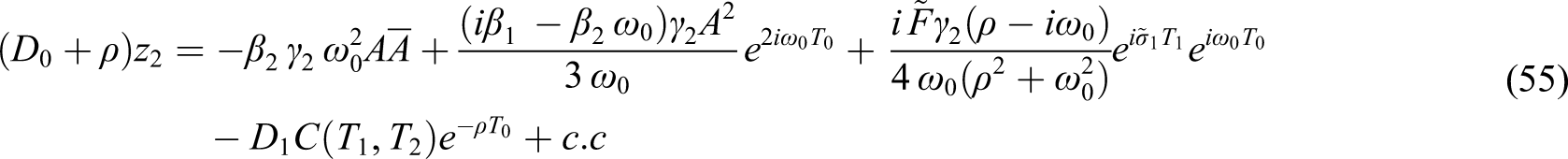
By using equations (47), (52), and (53) then substituting equation (41), one gets

$$\begin{array}{l}\left(D_0+\rho \right)z_2=-{\beta }_2\hspace{0.17em}{\gamma }_2\hspace{0.17em}{\omega }_0^{2}A\overline{A}+\frac{\left(i{\beta }_1\hspace{0.17em}-{\beta }_2\hspace{0.17em}{\omega }_0\right){\gamma }_2{A}^2}{3\hspace{0.17em}{\omega }_0}\hspace{0.17em}{e}^{2i{\omega }_0{T}_0}+\hspace{0.17em}\frac{i\hspace{0.17em}\tilde{F}{\gamma }_2\left(\rho -i{\omega }_0\right)}{4\hspace{0.17em}{\omega }_0\left({\rho }^2+{\omega }_0^2\right)}{e}^{i{\tilde{\sigma }}_1{T}_1}{e}^{i{\omega }_0{T}_0}\\ -D_{1}C\left(T_1,T_2\right)e^{-\rho T_0}+c.c\end{array}$$

(55)

For the purpose of eliminating the secular term in equation (55), the function $C\left(T_1,T_2\right)$ is then independent of $T_1$ . Therefore, one may write

$$C\left(T_1,T_2\right)=H\left(T_2\right)$$

(56)

The solution $z_2$ then becomes

$$z_2=-\frac{{\beta }_2\hspace{0.17em}{\gamma }_{2}A\overline{A}}{\rho }-\frac{{\gamma }_2\left(\rho -2i{\omega }_0\right)\left({\beta }_2{\omega }_0-i{\beta }_1\right)A^2}{3{\omega }_0\left({\rho }^2+4{\omega }_0^2\right)}{e}^{2i{\omega }_0{T}_0}+\frac{i\hspace{0.17em}\tilde{F}{\gamma }_2{\left(\rho -i{\omega }_0\right)}^2}{4\hspace{0.17em}{\omega }_0{\left({\rho }^2+{\omega }_0^2\right)}^2}{e}^{i{\tilde{\sigma }}_1{T}_1}{e}^{i{\omega }_0{T}_0}+c.c$$

(57)

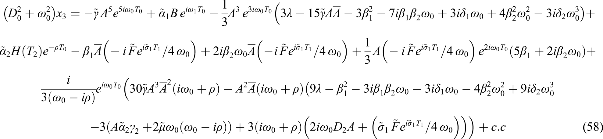
Substituting equations (45)–(47) and (53) and (54) into (42) and (43), one gets the following equations

$$\begin{array}{l}\left(D_0^2+{\omega }_0^2\right)x_3=-\tilde{\gamma }{A}^5{e}^{5i{\omega }_0{T}_0}+{\tilde{\alpha }}_{1}B\hspace{0.17em}{e}^{i{\omega }_1{T}_0}-\frac{1}{3}{A}^3\hspace{0.17em}{e}^{3i{\omega }_0{T}_0}(3\lambda +15\tilde{\gamma }A\overline{A}-3{\beta }_1^2-7i{\beta }_1{\beta }_2{\omega }_0+3i{\delta }_1{\omega }_0+4{\beta }_2^2{\omega }_0^2-3i{\delta }_2{\omega }_0^3)+\\ {\tilde{\alpha }}_{2}H\left(T_2\right)e^{-\rho T_0}-{\beta }_1\overline{A}\left(-i\hspace{0.17em}\tilde{F}{e}^{i{\tilde{\sigma }}_1{T}_1}/4\hspace{0.17em}{\omega }_0\right)+2i{\beta }_2{\omega }_0\overline{A}\left(-i\hspace{0.17em}\tilde{F}{e}^{i{\tilde{\sigma }}_1{T}_1}/4\hspace{0.17em}{\omega }_0\right)+\frac{1}{3}A\left(-i\hspace{0.17em}\tilde{F}{e}^{i{\tilde{\sigma }}_1{T}_1}/4\hspace{0.17em}{\omega }_0\right)\hspace{0.17em}{e}^{2i{\omega }_0{T}_0}\left(5{\beta }_1+2i{\beta }_2{\omega }_0\right)+\\ \frac{i}{3\left({\omega }_0-i\rho \right)}{e}^{i{\omega }_0{T}_0}(30\tilde{\gamma }{A}^3{\overline{A}}^2\left(i{\omega }_0+\rho \right)+A^2\overline{A}(i{\omega }_0+\rho )(9\lambda -{\beta }_1^2-3i{\beta }_1{\beta }_2{\omega }_0+3i{\delta }_1{\omega }_0-4{\beta }_2^2{\omega }_0^2+9i{\delta }_2{\omega }_0^3-\\ 3\left(A{\tilde{\alpha }}_2{\gamma }_2+2\tilde{\mu }{\omega }_0\left({\omega }_0-i\rho \right)\right)+3\left(i{\omega }_0+\rho \right)\left(2i{\omega }_0{D}_{2}A+\left({\tilde{\sigma }}_1\hspace{0.17em}\tilde{F}{e}^{i{\tilde{\sigma }}_1{T}_1}/4\hspace{0.17em}{\omega }_0\right)\right))+c.c\end{array}$$

(58)

and

$$\left(D_0^2+{\omega }_1^2\right)y_3={\tilde{\gamma }}_{1}A{e}^{i{\omega }_0{T}_0}+\left(-2i{\tilde{\mu }}_1{\omega }_1\hspace{0.17em}B-2i{\omega }_1{D}_{2}B\right)e^{i{\omega }_1{T}_0}+c.c$$

(59)

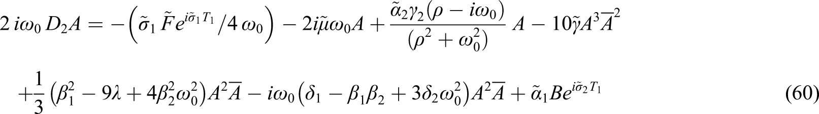
The solvability condition of equations (58) and (59) are

$$\begin{array}{l}2\hspace{0.17em}i{\omega }_0\hspace{0.17em}{D}_{2}A=-\left({\tilde{\sigma }}_1\hspace{0.17em}\tilde{F}{e}^{i{\tilde{\sigma }}_1{T}_1}/4\hspace{0.17em}{\omega }_0\right)-2i\tilde{\mu }{\omega }_{0}A+\frac{{\tilde{\alpha }}_2{\gamma }_2\left(\rho -i{\omega }_0\right)}{\left({\rho }^2+{\omega }_0^2\right)}A-10\tilde{\gamma }{A}^3{\overline{A}}^2+\frac{1}{3}({\beta }_1^2-9\lambda \\ +4{\beta }_2^2{\omega }_0^2)A^2\overline{A}-i{\omega }_0\left({\delta }_1-{\beta }_1{\beta }_2+3{\delta }_2{\omega }_0^2\right)A^2\overline{A}+{\tilde{\alpha }}_{1}B{e}^{i{\tilde{\sigma }}_2{T}_1}\end{array}$$

(60)

and

$$2i{\omega }_1{D}_{2}B=-2i{\tilde{\mu }}_1{\omega }_{1}B+{\tilde{\gamma }}_{1}A{e}^{-i{\tilde{\sigma }}_2{T}_1}$$

(61)

Therefore, the solutions of equations (58) and (59) after eliminating secular terms are

$$\begin{array}{l}{x}_3=\frac{\tilde{\gamma }{A}^5}{24{\omega }_0^2}{e}^{5i{\omega }_0{T}_0}+\frac{1}{24{\omega }_0^2}{A}^3\hspace{0.17em}{e}^{3i{\omega }_0{T}_0}\left(3\lambda +15\tilde{\gamma }A\overline{A}-3{\beta }_1^2-7i{\beta }_1{\beta }_2{\omega }_0+3i{\delta }_1{\omega }_0+4{\beta }_2^2{\omega }_0^2-3i{\delta }_2{\omega }_0^3\right)+\frac{{\tilde{\alpha }}_2}{\left({\omega }_0^2+{\rho }^2\right)}\\ H\left(T_2\right)e^{-\rho T_0}+\frac{i\hspace{0.17em}{\beta }_1\overline{A}\hspace{0.17em}\tilde{F}}{4\hspace{0.17em}{\omega }_0^3}{e}^{i{\tilde{\sigma }}_1{T}_1}+\frac{2{\beta }_2\overline{A}\hspace{0.17em}\tilde{F}}{4\hspace{0.17em}{\omega }_0^2}{e}^{i{\tilde{\sigma }}_1{T}_1}-\frac{i\hspace{0.17em}\tilde{F}}{36\hspace{0.17em}{\omega }_0^3}A\hspace{0.17em}{e}^{i{\tilde{\sigma }}_1{T}_1}{e}^{2i{\omega }_0{T}_0}\left(5{\beta }_1+2i{\beta }_2{\omega }_0\right)+c.c\end{array}$$

(62)

and

$$y_3=0$$

(63)

By using equations (47), (57), and (62), while substituting equation (44), one gets

$$\begin{array}{l}\left(D_0+\rho \right)z_3=\hspace{0.17em}\frac{\tilde{\gamma }{\gamma }_2{A}^5}{24{\omega }_0^2}{e}^{5i{\omega }_0{T}_0}+\frac{{\gamma }_2\hspace{0.17em}{A}^3}{24\hspace{0.17em}{\omega }_0^2}{e}^{3i{\omega }_0{T}_0}\left(3\lambda +15\tilde{\gamma }A\overline{A}-3{\beta }_1^2-7i{\beta }_1{\beta }_2{\omega }_0+3i{\delta }_1{\omega }_0+4{\beta }_2^2{\omega }_0^2\hspace{0.17em}-3i{\delta }_2{\omega }_0^3\right)\\ +\left(\frac{{\gamma }_2{\tilde{\alpha }}_2}{\left({\omega }_0^2+{\rho }^2\right)}H\left(T_2\right)-D_{2}H\left(T_2\right)\right)e^{-\rho T_0}-\frac{i\hspace{0.17em}\tilde{F}{\gamma }_2}{4\hspace{0.17em}\rho \hspace{0.17em}{\omega }_0^3}\overline{A}\hspace{0.17em}\left(-\rho {\beta }_1+2{\beta }_2{\omega }_0\left(i\rho +{\omega }_0\right)\right)\\ +e^{2i{\omega }_0{T}_0}{e}^{i\hspace{0.17em}{\tilde{\sigma }}_1{T}_1}\left(\frac{i\hspace{0.17em}\tilde{F}{\gamma }_2}{36\hspace{0.17em}{\omega }_0^3}\left(5{\beta }_1+2i{\beta }_2{\omega }_0\right)A\hspace{0.17em}-\frac{2\hspace{0.17em}i\hspace{0.17em}{\gamma }_2\tilde{F}\left(\rho -2i{\omega }_0\right)\left({\beta }_2{\omega }_0-i{\beta }_1\right))\hspace{0.17em}A}{12\hspace{0.17em}{\omega }_0^2\left({\rho }^2+4{\omega }_0^2\right)}\right)\\ +e^{i{\omega }_0{T}_0}\left(-\frac{{\gamma }_2\left(\rho -i{\omega }_0\right)D_{2}A\hspace{0.17em}}{{\rho }^2+{\omega }_0^2}\hspace{0.17em}+\frac{{\gamma }_2\hspace{0.17em}{\tilde{\sigma }}_1\hspace{0.17em}\tilde{F}{\left(\rho -i{\omega }_0\right)}^2\hspace{0.17em}}{4\hspace{0.17em}{\omega }_0{\left({\rho }^2+{\omega }_0^2\right)}^2}{e}^{i\hspace{0.17em}{\tilde{\sigma }}_1{T}_1}\right)+c.c\end{array}$$

(64)

The elimination of the secular term in equation (64) yields

$$H\left(T_2\right)=K\hspace{0.17em}Exp\left(\frac{{\tilde{\alpha }}_2{\gamma }_2{T}_2}{{\rho }^2+{\omega }_0^2}\right)=K\hspace{0.17em}Exp\left(\frac{{\alpha }_2{\gamma }_2{T}_2}{{\rho }^2+{\omega }_0^2}\right)$$

(65)

where $K$ is a constant of integration.

Consequently, the solution of $z_3$ of equation (64) gives

$$\begin{array}{l}{z}_3=\frac{\tilde{\gamma }{\gamma }_2\left(\rho -5i{\omega }_0\right)A^5\hspace{0.17em}}{4{\omega }_0^2\left({\rho }^2+25{\omega }_0^2\right)}{e}^{5i{\omega }_0{T}_0}+\frac{{\gamma }_2\left(\rho -3i{\omega }_0\right)A^3}{24\hspace{0.17em}{\omega }_0^2\left({\rho }^2+9{\omega }_0^2\right)}{e}^{3i{\omega }_0{T}_0}(3\lambda +15\tilde{\gamma }A\overline{A}-3{\beta }_1^2-7i{\beta }_1{\beta }_2{\omega }_0\begin{array}{l}+3i{\delta }_1{\omega }_0+\\ 4{\beta }_2^2{\omega }_0^2\hspace{0.17em}-3i{\delta }_2{\omega }_0^3\end{array})-\\ \frac{i\hspace{0.17em}\tilde{F}{\gamma }_2}{4\hspace{0.17em}{\rho }^2\hspace{0.17em}{\omega }_0^3}\overline{A}\hspace{0.17em}{e}^{i\hspace{0.17em}{\tilde{\sigma }}_1{T}_1}\hspace{0.17em}\left(-\rho {\beta }_1+2{\beta }_2{\omega }_0\left(i\rho +{\omega }_0\right)\right)+\frac{\left(\rho -2i{\omega }_0\right)}{\left({\rho }^2+4{\omega }_0^2\right)}{e}^{2i{\omega }_0{T}_0}{e}^{i\hspace{0.17em}{\tilde{\sigma }}_1{T}_1}\left(\begin{array}{l}\frac{i\hspace{0.17em}\tilde{F}{\gamma }_2}{36\hspace{0.17em}{\omega }_0^3}\left(5{\beta }_1+2i{\beta }_2{\omega }_0\right)A\hspace{0.17em}-\\ \frac{2\hspace{0.17em}i\hspace{0.17em}{\gamma }_2\tilde{F}\left(\rho -2i{\omega }_0\right)\left({\beta }_2{\omega }_0-i{\beta }_1\right)A}{12\hspace{0.17em}{\omega }_0^2\left({\rho }^2+4{\omega }_0^2\right)}\end{array}\right)\\ +\frac{\left(\rho -i{\omega }_0\right)}{\left({\rho }^2+{\omega }_0^2\right)}{e}^{i{\omega }_0{T}_0}\left(-\frac{{\gamma }_2\left(\rho -i{\omega }_0\right)D_{2}A\hspace{0.17em}}{{\rho }^2+{\omega }_0^2}\hspace{0.17em}+\frac{{\gamma }_2\hspace{0.17em}{\tilde{\sigma }}_1\hspace{0.17em}\tilde{F}{\left(\rho -i{\omega }_0\right)}^2\hspace{0.17em}}{4\hspace{0.17em}{\omega }_0{\left({\rho }^2+{\omega }_0^2\right)}^2}{e}^{i\hspace{0.17em}{\tilde{\sigma }}_1{T}_1}\right)+c.c\end{array}$$

(66)

In light of equation (34), the combination of equations (52) and (60) gives

$$\begin{array}{l}2\hspace{0.17em}i{\omega }_0\frac{dA}{dt}=\hspace{0.17em}\epsilon \frac{\tilde{F}}{2}{e}^{i\hspace{0.17em}{\tilde{\sigma }}_1{T}_1}+\hspace{0.17em}{\epsilon }^2(-\frac{{\tilde{\sigma }}_1\tilde{F}}{4\hspace{0.17em}{\omega }_0}{e}^{i\hspace{0.17em}{\tilde{\sigma }}_1{T}_1}-2i\tilde{\mu }{\omega }_{0}A-10\tilde{\gamma }{A}^3{\overline{A}}^2+\frac{1}{3}\left({\beta }_1^2-9\lambda +4{\beta }_2^2{\omega }_0^2\right)A^2\overline{A}\\ -i{\omega }_0\left({\delta }_1-{\beta }_1{\beta }_2+3{\delta }_2{\omega }_0^2\right)A^2\overline{A}+\frac{{\tilde{\alpha }}_2{\gamma }_2\left(\rho -i{\omega }_0\right)}{\left({\rho }^2+{\omega }_0^2\right)}A+{\tilde{\alpha }}_{1}B{e}^{i\hspace{0.17em}{\tilde{\sigma }}_2{T}_1})\end{array}$$

(67)

Once more, the mixture of equations (52) and (61) yields. and

$$2\hspace{0.17em}i{\omega }_1\frac{dB}{dt}={\epsilon }^2\left(-2i{\tilde{\mu }}_1{\omega }_{1}B++{\tilde{\gamma }}_{1}A{e}^{-i\hspace{0.17em}{\tilde{\sigma }}_2{T}_1}\right)$$

(68)

Equations (67) and (68) are coupled system of nonlinear ordinary differential equations of $A$ and $B$ with complex coefficients.

To investigate the solution of equations (67) and (68), following Nayfeh and Mook ⁴³ , it is suitable to use the polar form for the complex functions $A\left(T_1,T_2\right)$ and $B\left(T_1,T_2\right)$ as follows

$$A=\frac{\tilde{a}}{2}{e}^{i{\psi }_1},\hspace{0.17em}\text{and,}\hspace{1em}B=\frac{\tilde{b}}{2}{e}^{i{\psi }_2}$$

(69)

where $\tilde{a},\hspace{0.17em}\tilde{b},\hspace{0.17em}{\psi }_1$ , and ${\psi }_2$ are real functions on the time $t$ .

It is worthy to see that the functions $\tilde{a}$ and $\tilde{b}$ are the amplitudes, and that ${\psi }_1$ and ${\psi }_2$ are the phase angles of the polar solutions of the system and the corresponding controller, respectively.

As shown by Saeed and Kamel, ⁴¹ we may consider these functions as $a=\epsilon \hspace{0.17em}\tilde{a}$ and $b=\epsilon \hspace{0.17em}\tilde{b}$ .

The direct differentiation of the above functions gives

$$\dot{A}=\frac{\dot{\tilde{a}}}{2}{e}^{i{\psi }_1}+i\frac{\tilde{a}}{2}{\dot{\psi }}_1{e}^{i{\psi }_1},\hspace{0.17em}\text{and,}\hspace{1em}\dot{B}=\frac{\dot{\tilde{b}}}{2}{e}^{i{\psi }_2}+i\frac{\tilde{b}}{2}{\dot{\psi }}_1{e}^{i{\psi }_1}$$

(70)

By inserting equations (69) and (70) into (67) and (68), while restoring each scaled parameter to its original form (i.e., $\tilde{\mu }={\epsilon }^{-2}\mu$ , ${\tilde{\mu }}_1={\epsilon }^{-2}{\mu }_1$ , $\tilde{F}={\epsilon }^{-2}F$ , ${\tilde{\alpha }}_1={\epsilon }^{-2}{\tilde{\alpha }}_1$ , ${\tilde{\alpha }}_2={\epsilon }^{-2}{\alpha }_2$ , ${\tilde{\gamma }}_1={\epsilon }^{-2}{\gamma }_1$ , and $\tilde{\gamma }={\epsilon }^2\gamma$ ), then the separation of the real and imaginary parts yields

$$\dot{a}=\frac{\left({\beta }_1{\beta }_2-{\delta }_1-3{\delta }_2{\omega }_0^2\right)}{4}{a}^3-\frac{({\alpha }_2{\gamma }_2+2\mu \left({\rho }^2+{\omega }_0^2\right)}{\left({\rho }^2+{\omega }_0^2\right)}a-\frac{F\left({\sigma }_1-2{\omega }_0\right)}{2{\omega }_0^2}\sin \hspace{0.17em}{\theta }_1+\frac{{\alpha }_1}{{\omega }_0}b\hspace{0.17em}\sin \hspace{0.17em}{\theta }_2$$

(71)

$$a{\dot{\psi }}_1=\frac{\left(9\lambda -{\beta }_1^2-4{\beta }_2^2{\omega }_0^2\right)}{12{\omega }_0}{a}^3+\frac{5\gamma }{8{\omega }_0}{a}^5-\frac{\rho {\alpha }_2{\gamma }_2}{{\omega }_0\left({\rho }^2+{\omega }_0^2\right)}a+\frac{F\left({\sigma }_1-2{\omega }_0\right)}{2{\omega }_0^2}\cos \hspace{0.17em}{\theta }_1-\frac{{\alpha }_1}{{\omega }_0}b\hspace{0.17em}\cos \hspace{0.17em}{\theta }_2$$

(72)

$$\dot{b}=-\frac{{\gamma }_1}{{\omega }_1}a\hspace{0.17em}\sin \hspace{0.17em}{\theta }_2-2{\mu }_{1}b$$

(73)

and

$$b{\dot{\psi }}_2=-\frac{{\gamma }_1}{{\omega }_1}a\hspace{0.17em}\cos \hspace{0.17em}{\theta }_2$$

(74)

where ${\theta }_1={\sigma }_{1}t-{\psi }_1$ and ${\theta }_2={\sigma }_{2}t-{\psi }_1+{\psi }_2$ .

The autonomous system of equations (71)–(74) gives the governing equations for the amplitude–phase modulating.

In the next Section, the above coupled system of nonlinear ordinary differential equations with real coefficients, for simplicity, may be solved via the steady-state solution.

Steady-State Solution

The above autonomous system of equations that is given in equations (71)–(74) will be solved by using the steady-state solution. For this purpose, one may write

$$\dot{a}={\dot{\theta }}_1=\dot{b}={\dot{\theta }}_2=0$$

(75)

Therefore, ${\dot{\psi }}_1={\sigma }_1$ and ${\dot{\psi }}_2={\sigma }_1-{\sigma }_2$ . The substitution of equations (75) into (71)–(74) leads to

$$\frac{\left({\beta }_1{\beta }_2-{\delta }_1-3{\delta }_2{\omega }_0^2\right)}{4}{a}^3-\frac{({\alpha }_2{\gamma }_2+2\mu \left({\rho }^2+{\omega }_0^2\right)}{\left({\rho }^2+{\omega }_0^2\right)}a=\frac{F\left({\sigma }_1-2{\omega }_0\right)}{2{\omega }_0^2}\sin \hspace{0.17em}{\theta }_1-\frac{{\alpha }_1}{{\omega }_0}b\hspace{0.17em}\sin \hspace{0.17em}{\theta }_2$$

(76)

$$\left({\sigma }_1+\frac{\rho {\alpha }_2{\gamma }_2}{{\omega }_0\left({\rho }^2+{\omega }_0^2\right)}\right)a-\frac{\left(9\lambda -{\beta }_1^2-4{\beta }_2^2{\omega }_0^2\right)}{12{\omega }_0}{a}^3-\frac{5\gamma }{8{\omega }_0}{a}^5=\frac{F\left({\sigma }_1-2{\omega }_0\right)}{2{\omega }_0^2}\cos \hspace{0.17em}{\theta }_1-\frac{{\alpha }_1}{{\omega }_0}b\hspace{0.17em}\cos \hspace{0.17em}{\theta }_2$$

(77)

$$2{\mu }_{1}b=-\frac{{\gamma }_1}{{\omega }_1}a\hspace{0.17em}\sin \hspace{0.17em}{\theta }_2$$

(78)

and

$$\left({\sigma }_1-{\sigma }_2\right)b=-\frac{{\gamma }_1}{{\omega }_1}a\hspace{0.17em}\cos \hspace{0.17em}{\theta }_2$$

(79)

The coupling equations (78) and (79) yields

$$b^2=\frac{{\gamma }_1^2}{\left(4{\mu }_1^2+{\left({\sigma }_1-{\sigma }_2\right)}^2\right){\omega }_1^2}{a}^2$$

(80)

On the other hand, the combination of equations (76)–(79) gives

$$\begin{array}{l}(\frac{\left({\beta }_1{\beta }_2-{\delta }_1-3{\delta }_2{\omega }_0^2\right)}{4}{a}^3{-\left(\frac{({\alpha }_2{\gamma }_2+2\mu \left({\rho }^2+{\omega }_0^2\right)}{\left({\rho }^2+{\omega }_0^2\right)}+\frac{2{\alpha }_1{\mu }_1{\gamma }_1}{\left(4{\mu }_1^2+{\left({\sigma }_1-{\sigma }_2\right)}^2\right){\omega }_0{\omega }_1}\right)a)}^2+(({\sigma }_1+\frac{\rho {\alpha }_2{\gamma }_2}{{\omega }_0\left({\rho }^2+{\omega }_0^2\right)}\\ {-\frac{{\alpha }_1{\gamma }_1\left({\sigma }_1-{\sigma }_2\right)}{\left(4{\mu }_1^2+{\left({\sigma }_1-{\sigma }_2\right)}^2\right){\omega }_0{\omega }_1})a-\frac{\left(9\lambda -{\beta }_1^2-4{\beta }_2^2{\omega }_0^2\right)}{12{\omega }_0}{a}^3-\frac{5\gamma }{8{\omega }_0}{a}^5)}^2=\frac{F^2{\left({\sigma }_1-2{\omega }_0\right)}^2}{4{\omega }_0^4}{a}^2\end{array}$$

(81)

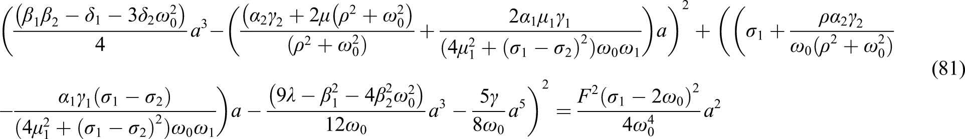
Equations (80) and (81) represent the frequency response equations (FREs). They are used to describe steady-state solutions of the system.

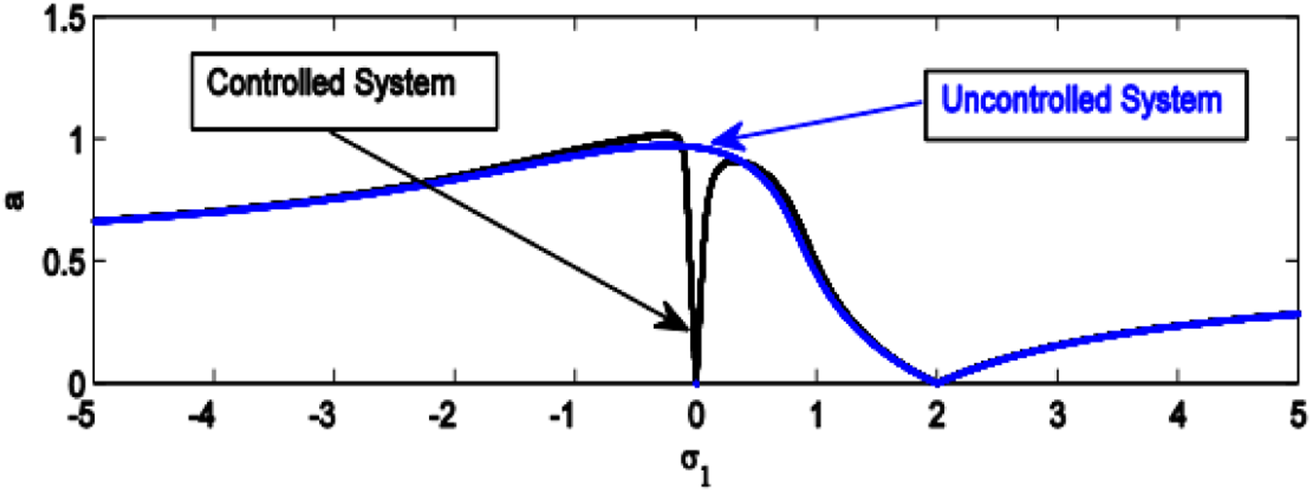
The MATLAB software will be utilized to sketch the coupled transcendental equations (80) and (81). The utilized data are given in Conclusions. In what follows, the oscillator amplitude against ${\sigma }_1$ gives the FRC. To study the importance of adding the controller, a comparison of FRC is made between the uncontrolled and the controlled systems as shown in Figure 10. From this comparison, we find that when ${\sigma }_1=0$ (i.e., at the state of resonance), the amplitude of the vibration is the highest as shown by the blue curve of the uncontrolled system. Simultaneously, the amplitude decreases completely in this region as shown by the black curve of the controlled system. This confirms the efficiency of the controller in reducing the vibration in the state of resonance. Therefore, the neighboring region ${\sigma }_1=0$ is called the suppression bandwidth of vibration because there are two peaks to its right and left. Finally, at ${\sigma }_1=2$ , we noticed that there was no evident vibration before adding the controller, and still there is no vibration after adding the controller.

Figure 10.

Comparison between the frequency response curves of an uncontrolled system and controlled system.

The FRC of the NIPPF controlled system is illustrated in Figure 11, where the left graph represents the oscillator amplitude $a$ versus ${\sigma }_1$ , and the right graph signifies the controller amplitude $b$ versus ${\sigma }_1$ .

Figure 11.

Frequency response curve of nonlinear integrated positive position feedback controlled oscillator system at ${\sigma }_2=0$ (a) ( $a$ against ${\sigma }_1$ ) and (b) ( $b$ against ${\sigma }_1$ ).

It is evident from this figure that the control connection added to the system leads to damping the lateral vibrations in the area around the bandwidth region near ${\sigma }_1=0$ . Therefore, the vibration can be optimally damped when placed at ${\sigma }_1={\sigma }_2=0$ . These results are compatible with those obtained earlier by Amer et al. ³⁸ and El-Sayed and Bauomy ⁴² for FRC after using the NIPPF controller.

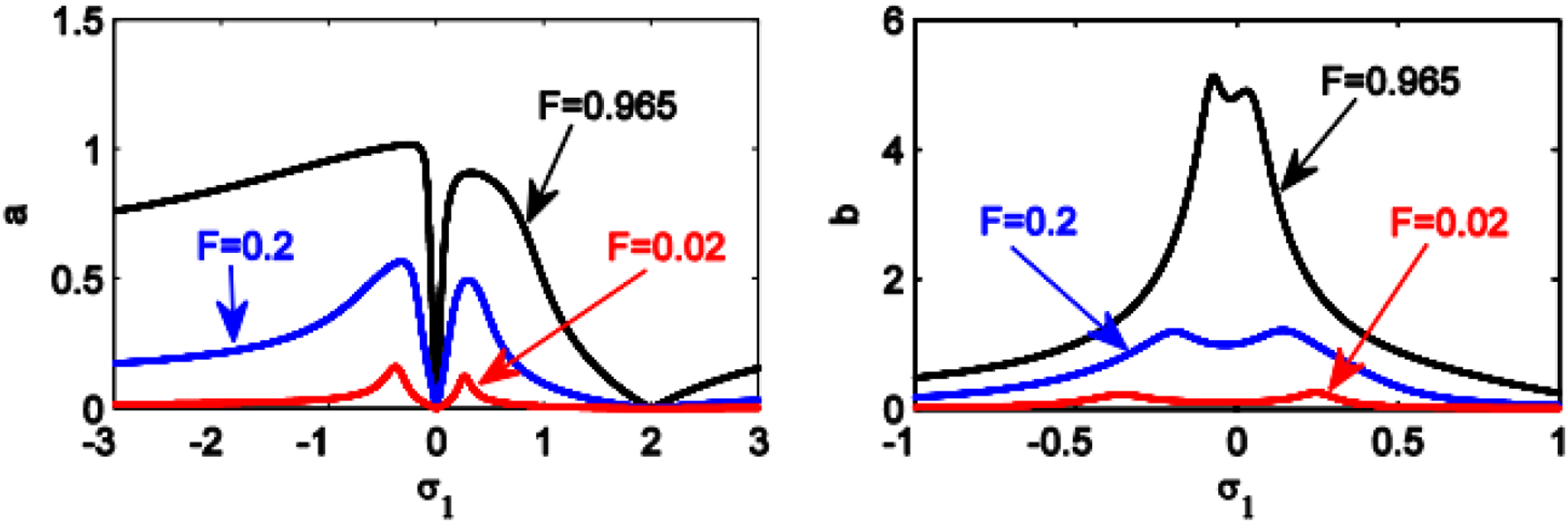
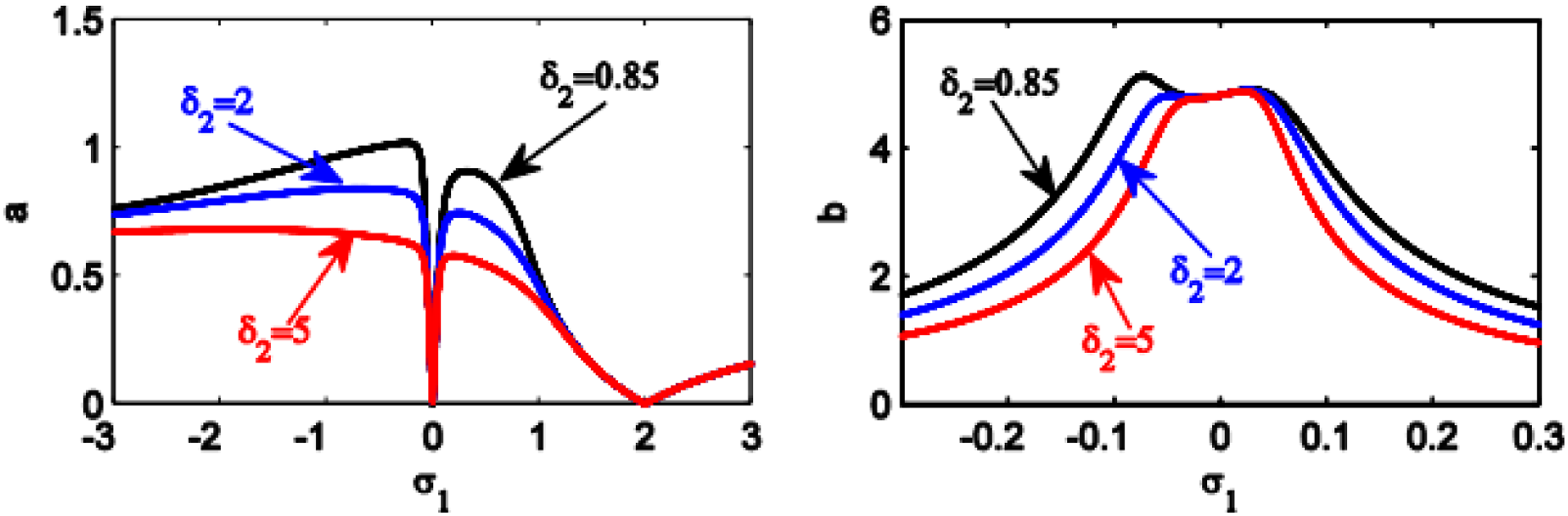
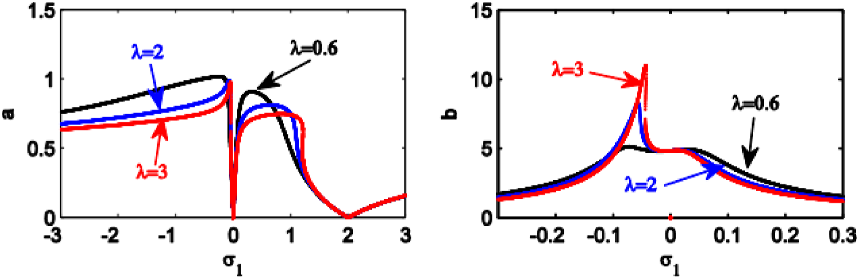
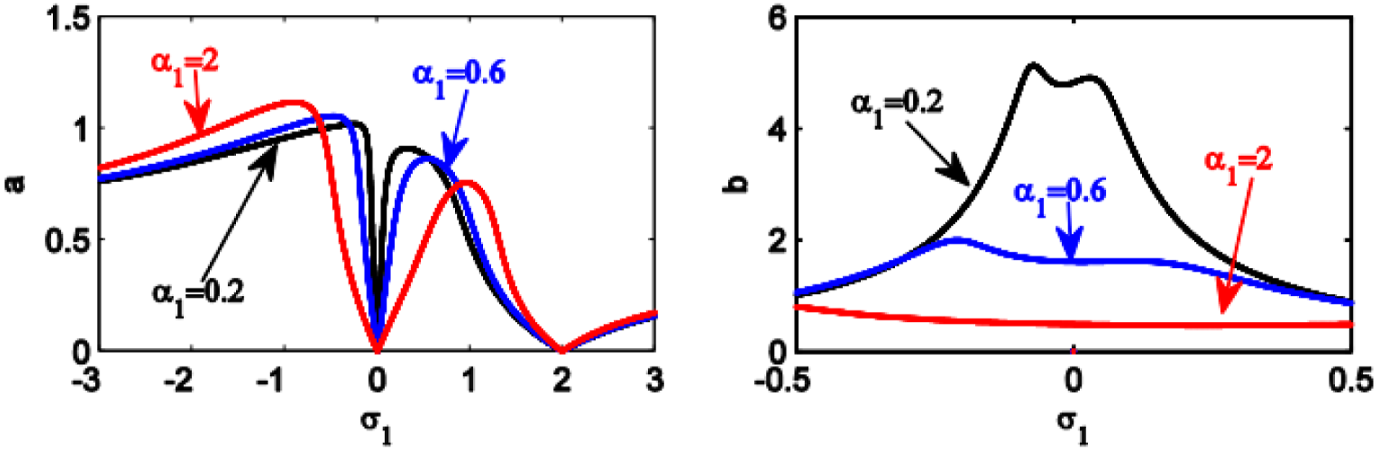
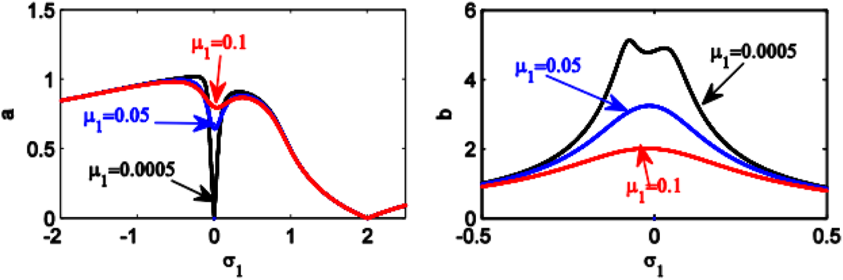
In the following figures, the effects of different controller and system parameters on FRC will be illustrated in the primary and internal resonance. Figure 12 shows the influence of FRC on the oscillator for different values of $F$ . The decrease of $F$ leads to a decrease in the amplitude and an increase in the suppression bandwidth of vibration. It is concluded that small values of $F$ , a larger region of the suppression bandwidth of vibration, are obtained. When reducing the value $\mu$ , the amplitudes of the two peaks on the left and right of the suppression bandwidth of the vibration region decrease. Furthermore, the right amplitude jump phenomenon occurs for both the oscillator and controller as shown in Figure 13. Figure 14 shows the effect of ${\omega }_0$ . It is observed that by increasing ${\omega }_0$ , the zero solution (i.e., at ${\sigma }_1=2$ ) shifts to the right. Moreover, the amplitude of the oscillator and the controller decreases.

Figure 12.

Controlled hybrid Rayleigh–Van der Pol–Duffing oscillator of frequency response curves at changed values of the external force $\left(F\right)$ .

Figure 13.

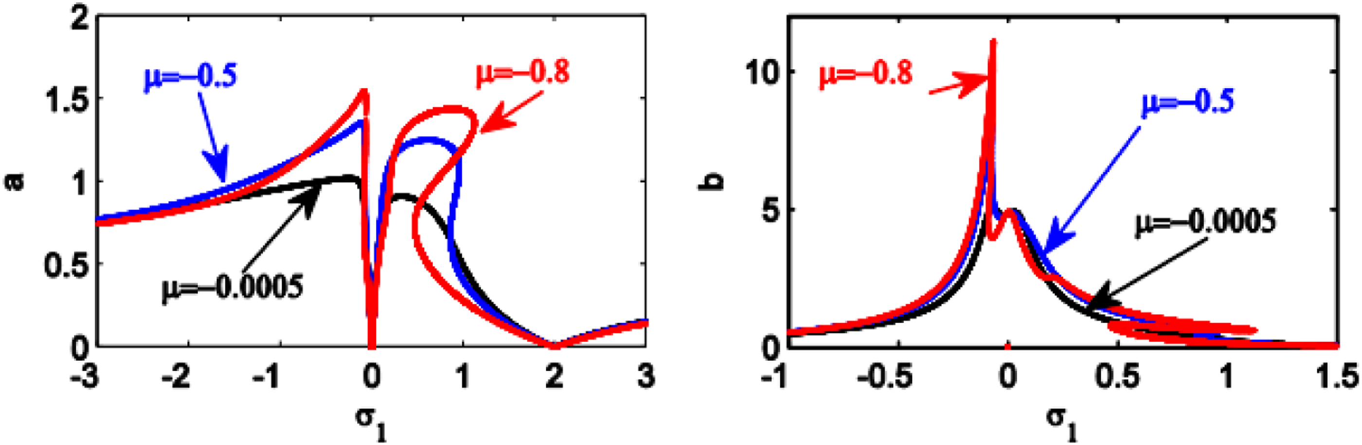
Controlled hybrid Rayleigh–Van der Pol–Duffing oscillator of frequency response curves at changed values of the linear damping coefficient $\left(\mu \right)$ .

Figure 14.

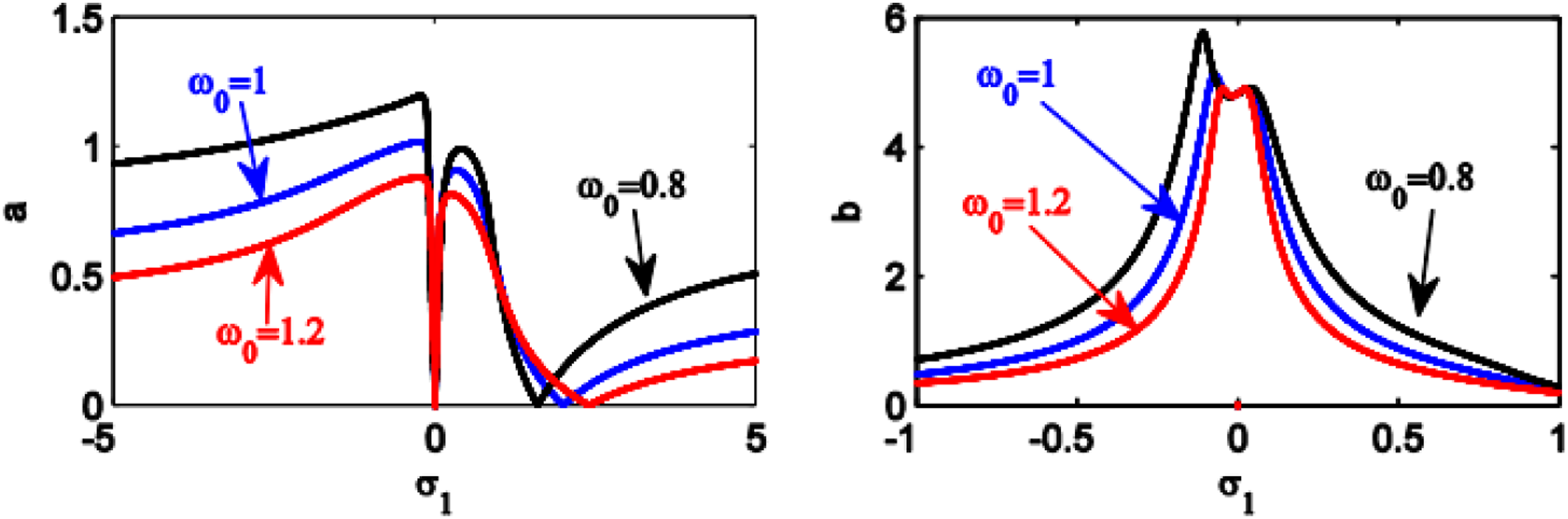
Controlled hybrid Rayleigh–Van der Pol–Duffing oscillator of frequency response curves at changed values of the natural frequency $\left({\omega }_0\right)$ .

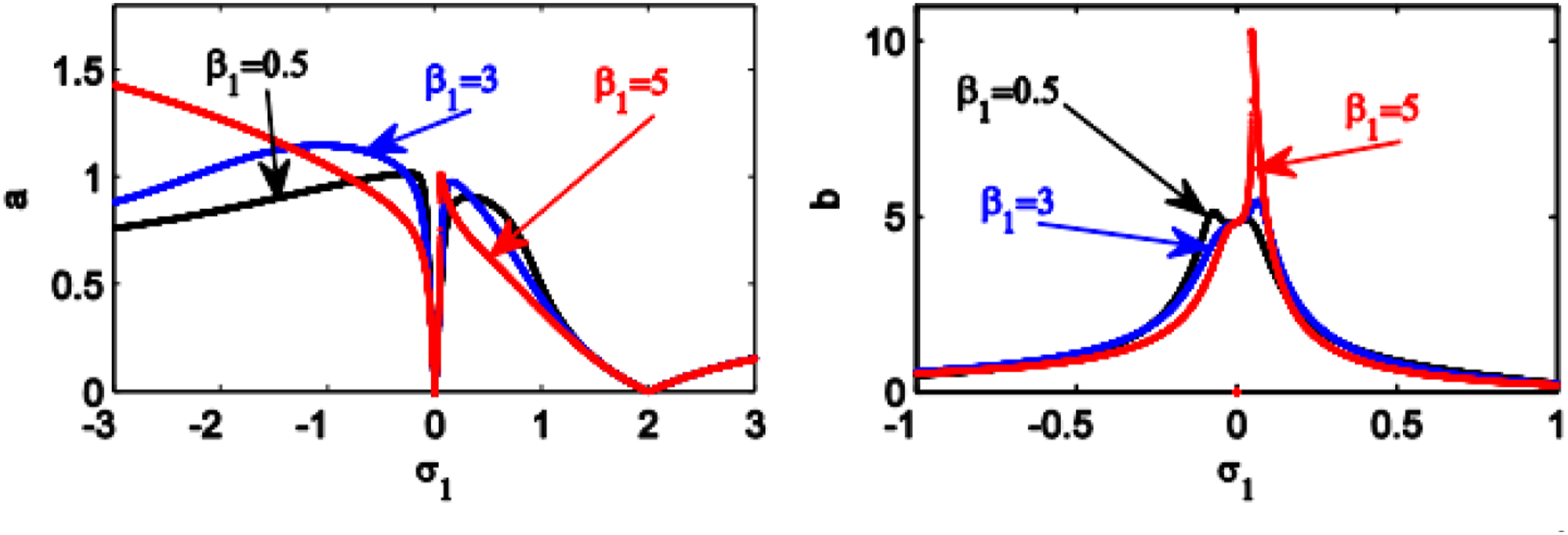
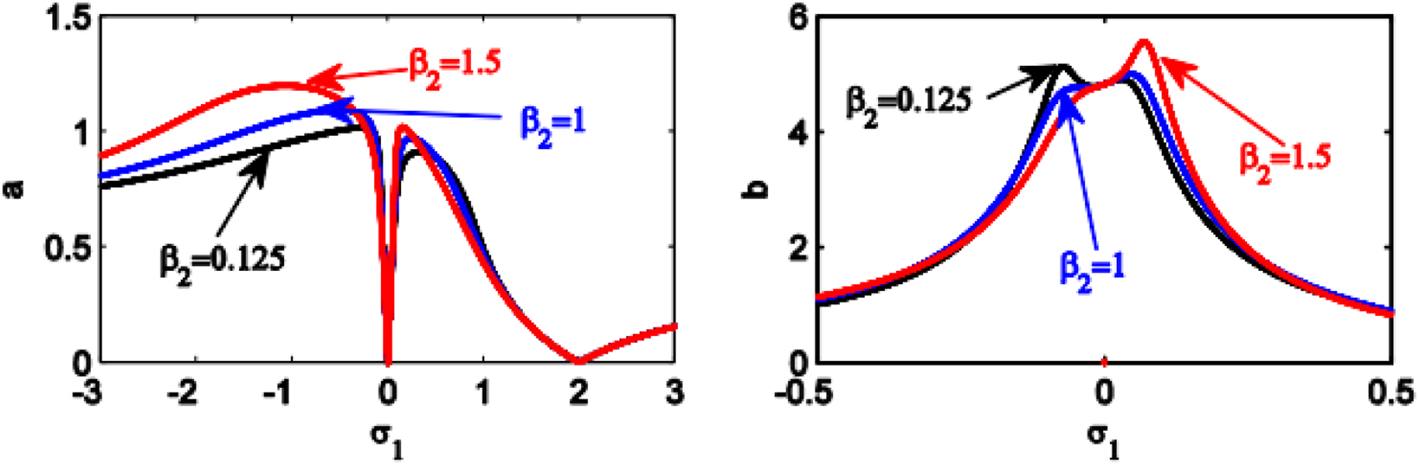
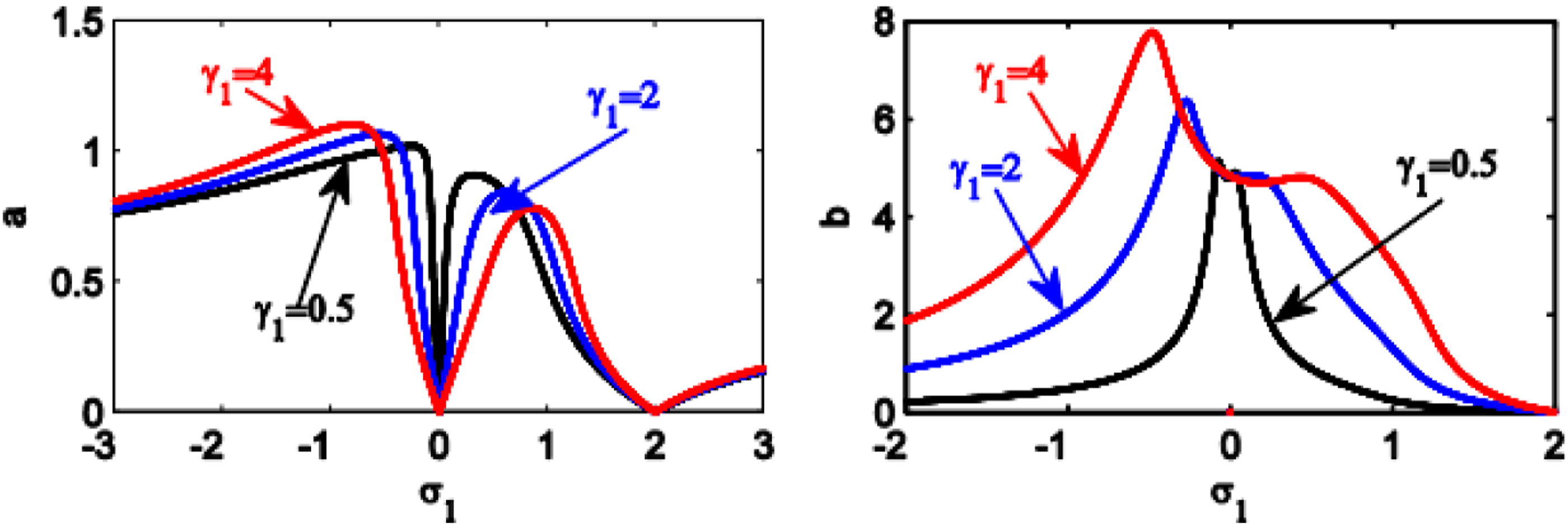
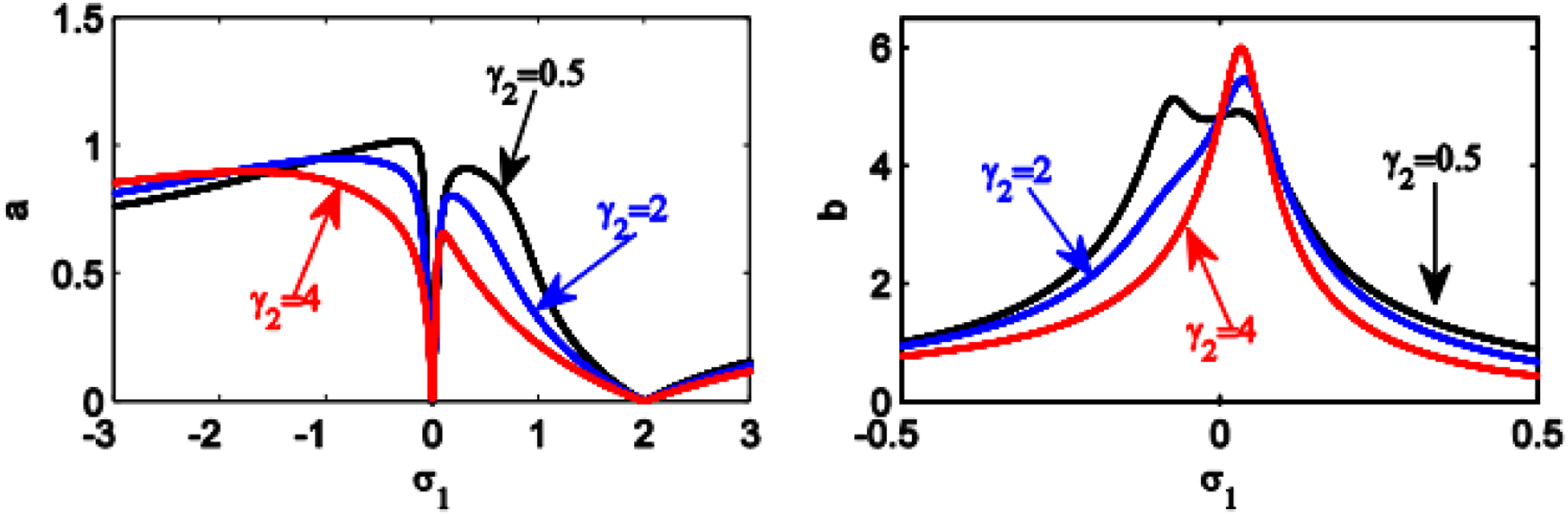
In Figures 15 and 16, the effect ${\beta }_1$ and ${\beta }_2$ is evident. At large values of ${\beta }_1$ and ${\beta }_2$ , the amplitude of the left and right peaks of the system increases. Furthermore, the width of the right peak shrinks while the width of the left peak of the system expands. As for the control, the right peak rises and the left peak goes down.

Figure 15.

Controlled hybrid Rayleigh–Van der Pol–Duffing oscillator of frequency response curves at changed values of the impure quadratic damping coefficient $\left({\beta }_1\right)$ .

Figure 16.

Controlled hybrid Rayleigh–Van der Pol–Duffing oscillator of frequency response curves at changed values of the pure quadratic damping coefficient $\left({\beta }_2\right)$ .

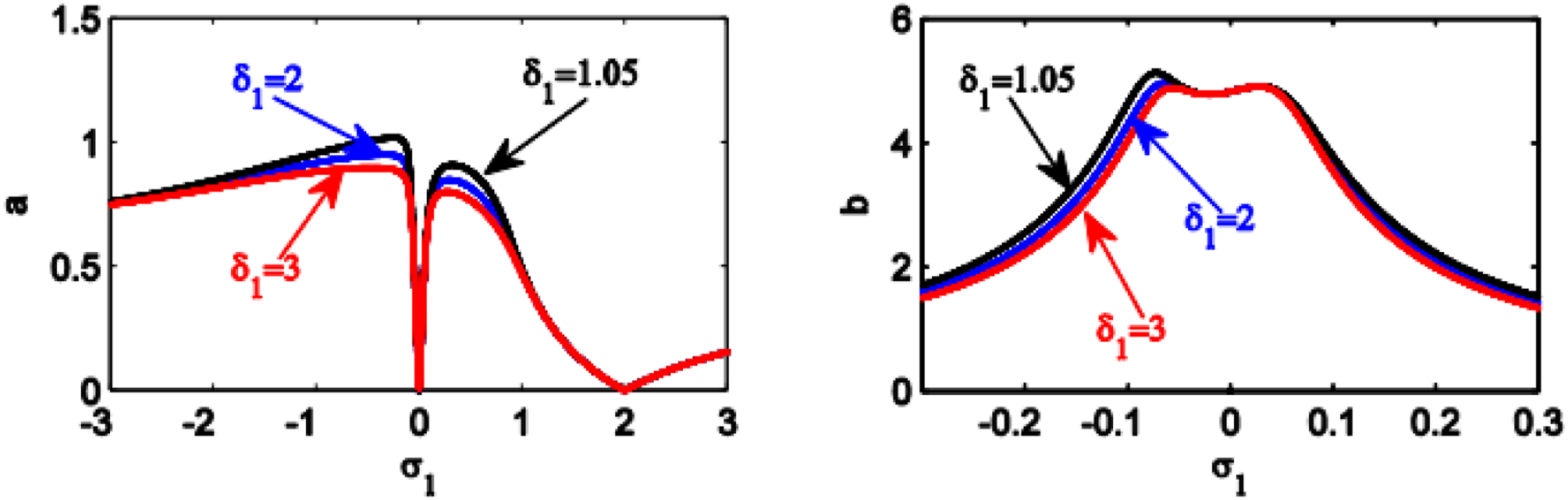
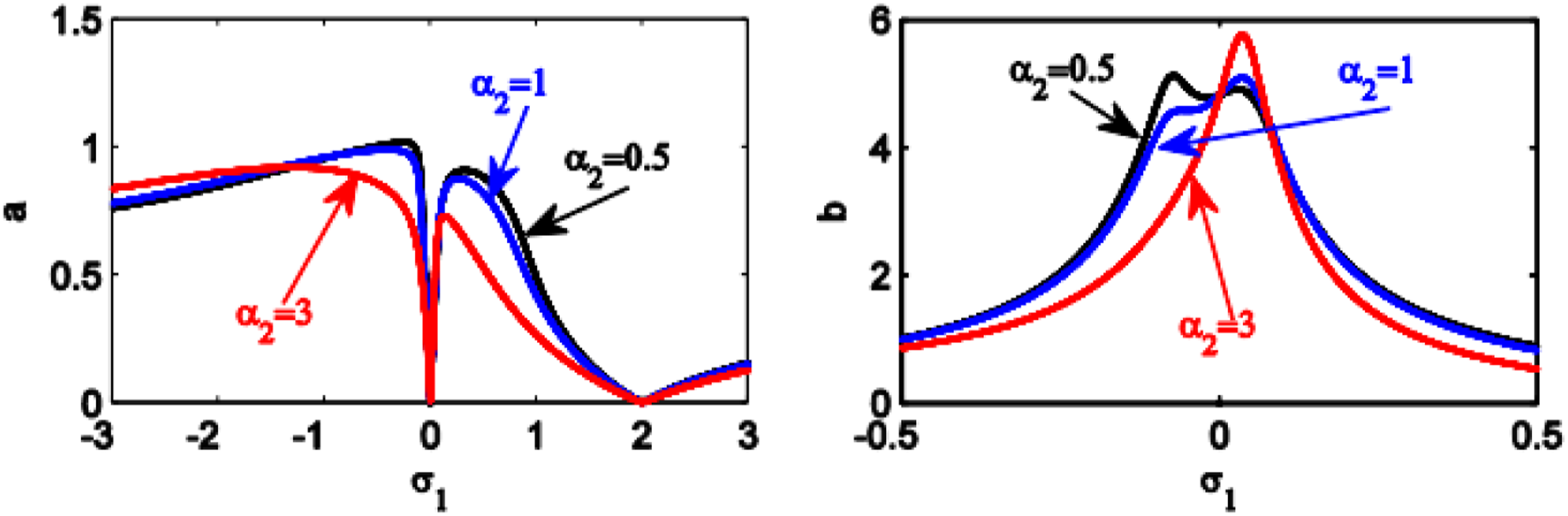
An increase in the values ${\delta }_1$ and ${\delta }_2$ leads to a reduction of the amplitude of the oscillator and the controller shown in Figures 17 and 18. When the values of $\lambda$ and $\gamma$ are high, the left peak shrinks and the right peak of the system expands. As for the controller, the left peak rises and the right peak disappears as clearly shown in Figures 19 and 20.

Figure 17.

Controlled hybrid Rayleigh–Van der Pol–Duffing oscillator of frequency response curves at changed values of the impure cubic damping coefficient $\left({\delta }_1\right)$ .

Figure 18.

Controlled hybrid Rayleigh–Van der Pol–Duffing oscillator of frequency response curves at changed values of the pure cubic damping coefficient $\left({\delta }_2\right)$ .

Figure 19.

Controlled hybrid Rayleigh–Van der Pol–Duffing oscillator of frequency response curves at changed values of the cubic nonlinear Duffing coefficient $\left(\lambda \right)$ .

Figure 20.

Controlled hybrid Rayleigh–Van der Pol–Duffing oscillator of frequency response curves at changed values of the quintic nonlinear Duffing coefficient $\left(\gamma \right)$ .

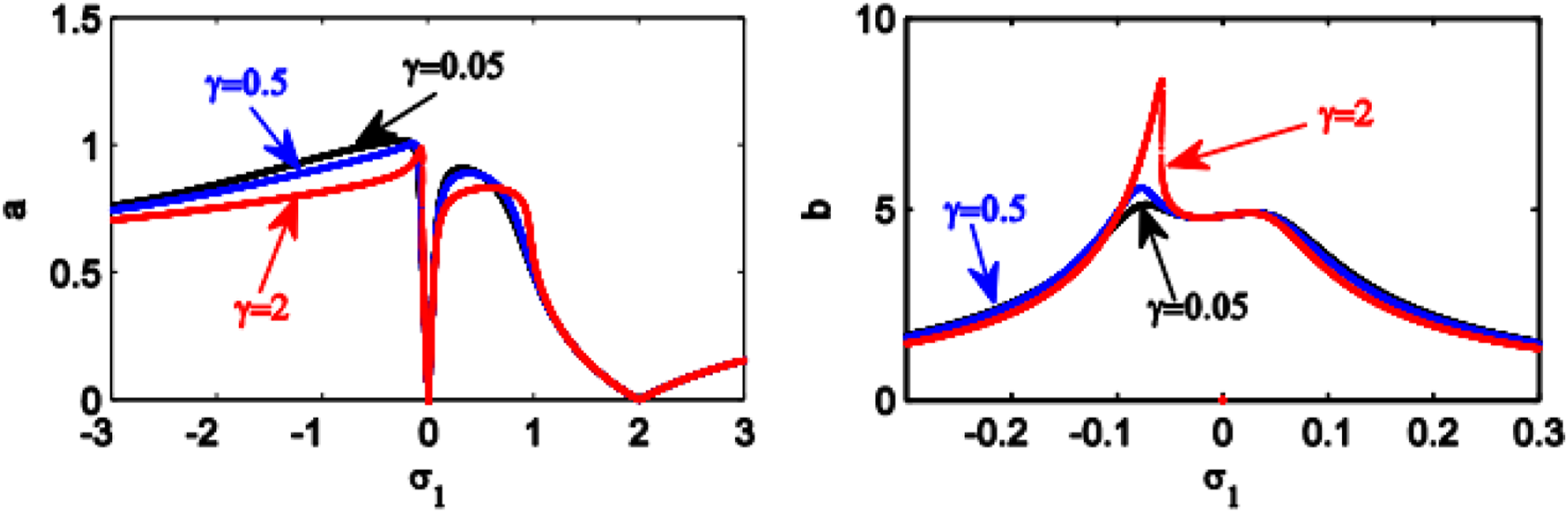
From Figure 21, it is noticed that the area of the suppression bandwidth of vibration for both the oscillator and the controller expands to the large value of ${\alpha }_1$ . In addition, the left amplitude peak raises while the right amplitude peak of the system decreases, but the amplitude of the controller decreases.

Figure 21.

Controlled hybrid Rayleigh–Van der Pol–Duffing oscillator of frequency response curves at changed values of the feedback gain $\left({\alpha }_1\right)$ .

As for Figure 22, it becomes clear that with the great value of ${\gamma }_1$ , the area of the suppression bandwidth of vibration expands. In addition, the left amplitude peak rises and the right amplitude peak decreases for both the oscillator and the controller. In Figures 23 and 24, the two peaks of the oscillator decrease when the values of both ${\alpha }_2$ and ${\gamma }_2$ increase. In addition, the left peak of the controller decreases and the right peak increases. When the value of ${\mu }_1$ increases, the region of the suppression bandwidth of vibration expands. Also, it is noticed that the amplitude value increases at the resonance case (i.e., ${\sigma }_1=0$ ) as shown in Figure 25. Therefore, ${\mu }_1$ should be as small as possible.

Figure 22.

Controlled hybrid Rayleigh–Van der Pol–Duffing oscillator of frequency response curves at changed values of the controller gain $\left({\gamma }_1\right)$ .

Figure 23.

Controlled hybrid Rayleigh–Van der Pol–Duffing oscillator of frequency response curves at changed values of the feedback gain $\left({\alpha }_2\right)$ .

Figure 24.

Controlled hybrid Rayleigh–Van der Pol–Duffing oscillator of frequency response curves at changed values of the controller gain $\left({\gamma }_2\right)$ .

Figure 25.

Controlled hybrid Rayleigh–Van der Pol–Duffing oscillator of frequency response curves at changed values of the linear damping coefficient of controller $\left({\mu }_1\right)$ .

The effect of the detaining parameter ${\sigma }_2$ on the FRC is shown in Figure 26. Here, in the left graph, it is clear that the minimum vibration amplitudes are formed when ${\sigma }_1={\sigma }_2$ . Accordingly, if ${\sigma }_1={\sigma }_2$ , the controller will reduce the vibration amplitude of system as less as possible. Consequently, the best work conditions of the planned controller are when ${\omega }_0={\omega }_1=\omega$ . Thus, we can adjust the natural frequencies of the controllers as ${\omega }_0={\omega }_1=\omega$ to eliminate the side vibrations of the system. Therefore, the proposed NIPPF control at any spinning speed can eliminate system vibrations.

Figure 26.

Controlled hybrid Rayleigh–Van der Pol–Duffing oscillator of frequency response curves at changed values of the detaining parameter $\left({\sigma }_2\right)$ .

There are similar results for the effects of different controller and system parameters on the controlled FRC made by Amer et al., ³⁸ El-Sayed and Bauomy, ⁴² Amer et al. ⁴⁴ and Saeed et al. ⁴⁵

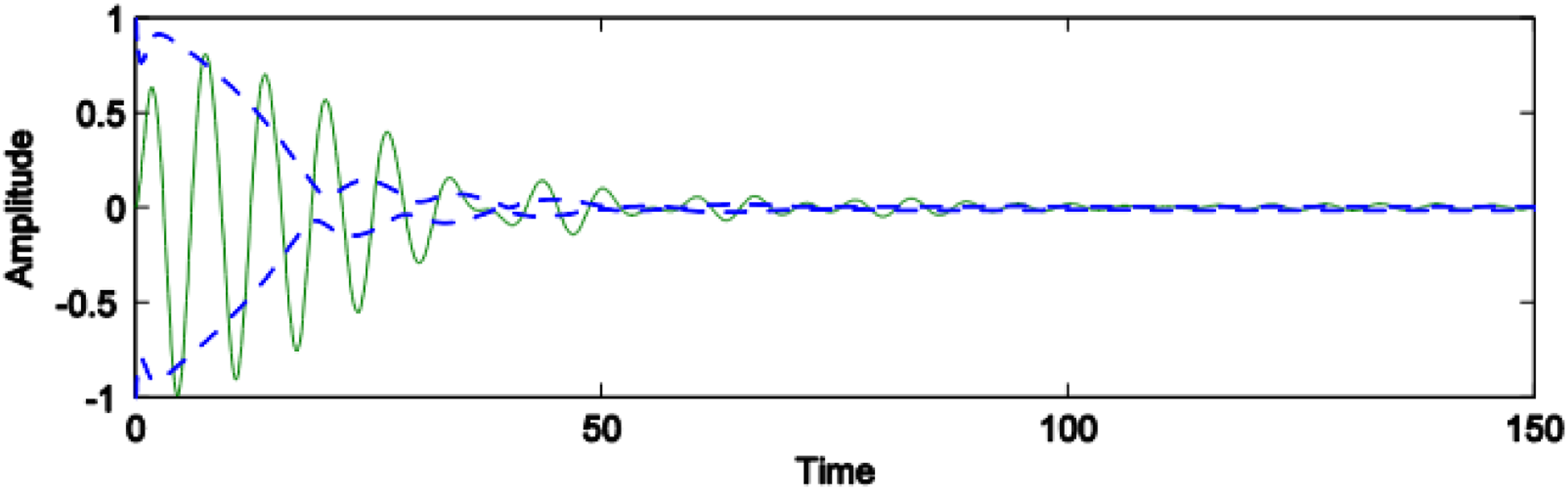
A comparison of time history between the numerical solution of equations (28)–(30) and the analytical solution of equation (71)–(74), when using the steady-state condition (i.e., $\dot{a}={\dot{\theta }}_1=\dot{b}={\dot{\theta }}_2=0$ ), was done as in Figure 27. In this figure, the numerical solution of the basic system after adding the NIPPF controller is indicated by continuous lines, while the analytical solution is represented by dashed lines. It is obvious that there is a good compatibility between both the numerical and analytical solutions, which confirms the accuracy of our solution.

Figure 27.

Time history between an analytic solution (solid curve) and numerical solution (dashed curve) at primary and internal resonance case ( $\omega ={\omega }_0$ and ${\omega }_1={\omega }_0$ ).

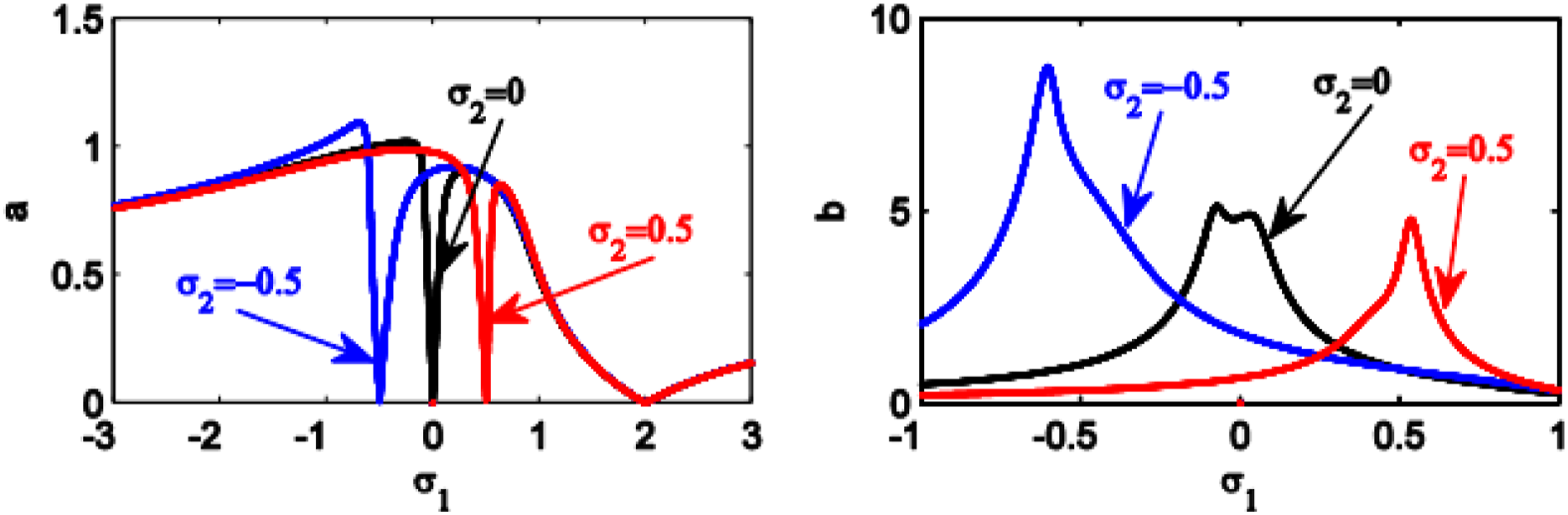
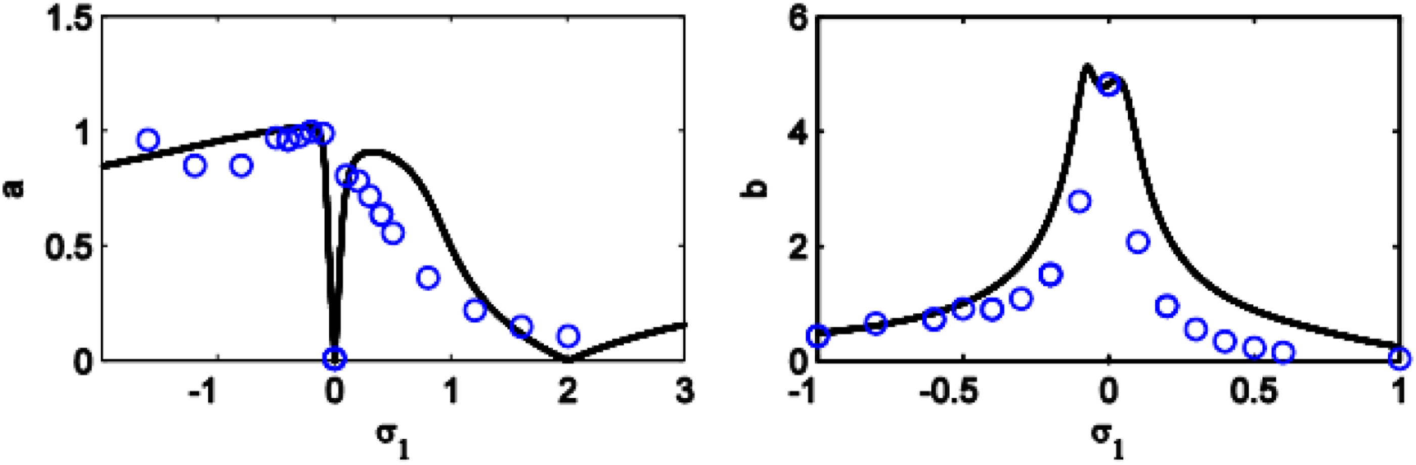
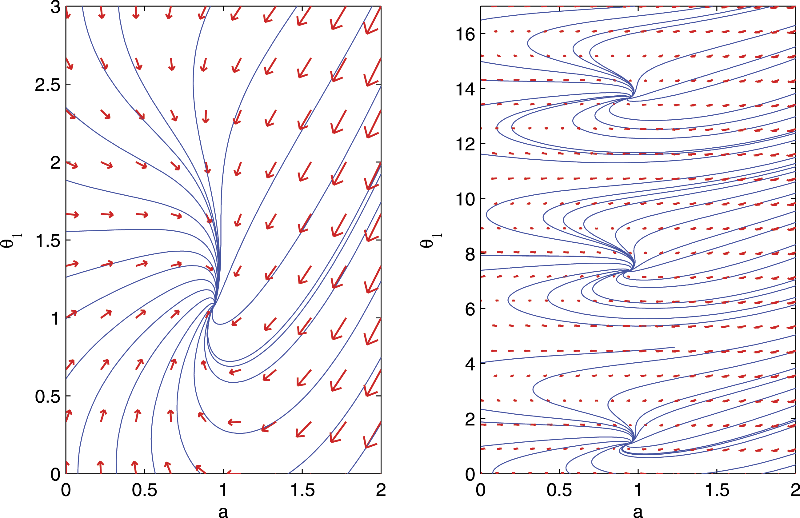
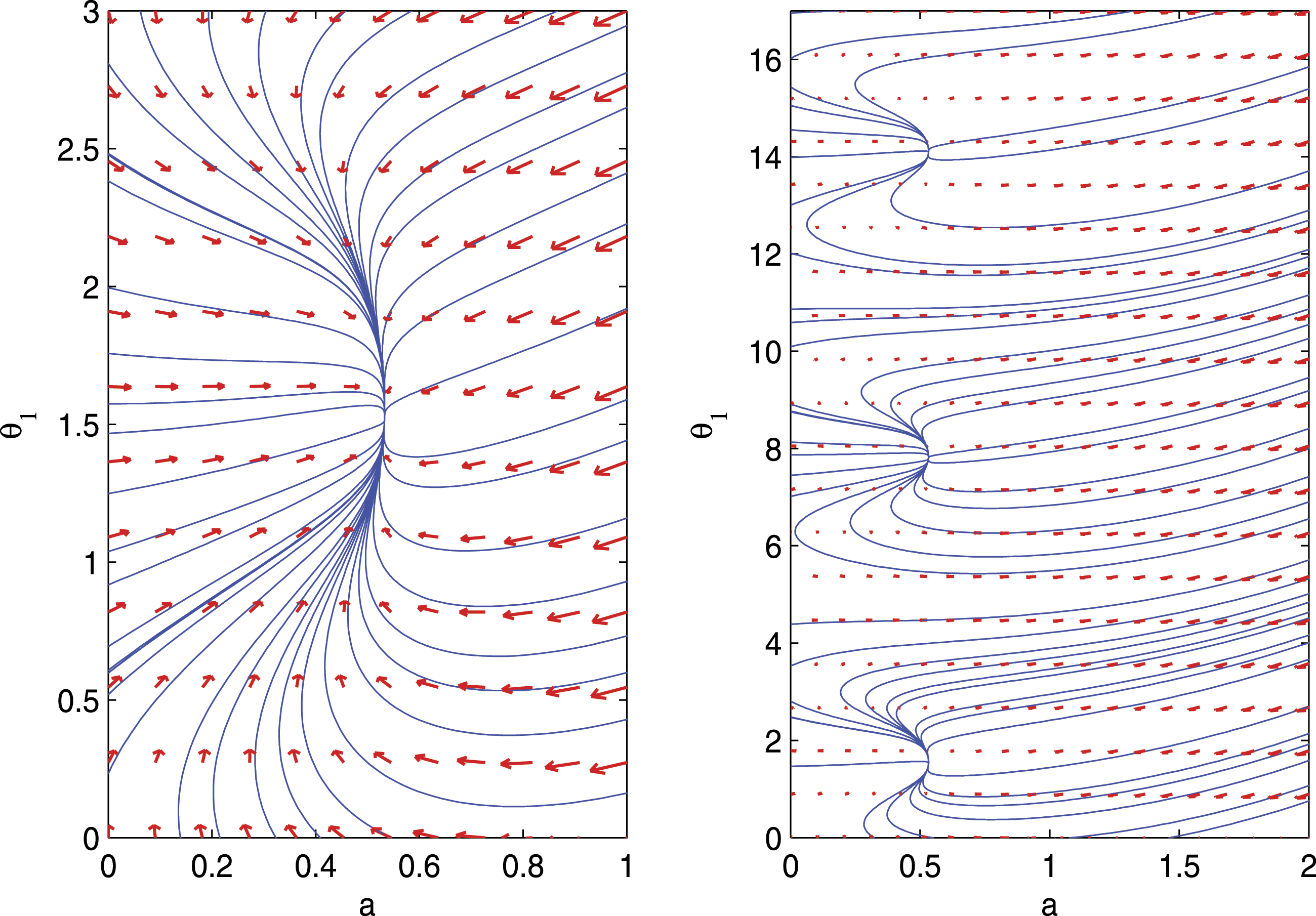
Moreover, by comparing the FRC for both numerical and analytical solutions as in Figure 28 at the studied resonance case, it is noticed that the predictions of the analytical solution based on the numerical solution are very precise. To study the stability of the oscillator before adding the controller, we made a study of the phase plane as shown in Figures 29 and 30. This study is applied by the equations of amplitude–phase modulating when putting $b=0$ and ${\theta }_2=0$ . As noted in Figure 29, critical points are formed at (0.938647, 1.07276+6.28319 h), (h $\in$ Integers) when choosing $F=0.965$ . Because critical point eigenvalues ( ${\lambda }_1$ and ${\lambda }_2$ ) are ${\lambda }_1={\overline{\lambda }}_2=a+ib$ , $a<0$ and $b>0$ , thus their classification is staple spiral. By contrast, when the value of the external force is $F=0.2$ , the critical points are formed in (0.532658,1.51632+6.28319 r), (r $\in$ Integers) and the eigenvalues for them are ${\lambda }_1<{\lambda }_2<0$ , thus their classifications are staple proper node as clear in Figure 30.

Figure 28.

Frequency response curves comparison between both analytic solutions with line and RK4 with circle.

Figure 29.

Phase plane of the uncontrolled oscillator at ${\sigma }_1=0,\hspace{0.17em}F=0.965$ .

Figure 30.

Phase plane of the uncontrolled oscillator at ${\sigma }_1=0,\hspace{0.17em}F=0.2$ .

Conclusions

In light of the potential applications of the HRVD in diverse domains of science, physics, and engineering, the current article aims to investigate the problem at hand. An analytic bounded solution by means of P-L technique is obtained. To validate this approach, a graphical representation between the P-L and RK4 is made to ensure the convenience in handling the P-L technique. Additionally, the linearized stability is achieved near the equilibrium points of the HRVD and the phase portraits are plotted. It is more convenient to suppress the vibration that is subjected from the external force. A numerical comparison of the RK4 of the time history between NIPPF, IRC, and PPF is made. As seen in Figure 8, it is found that the best controller, in light the suppression of the vibration in a smaller time, is the NIPPF. Consequently, the NIPPF controller is introduced to control nonlinear vibrations of the external excitation. The proposed controller equations are included and linked to the oscillator equation with three equations or three degrees of freedom as given in equations (28)–(30). These equations are studied analytically by using the multiple scales method from which the FREs are obtained near the primary resonance $\omega ={\omega }_0$ and the internal resonance ${\omega }_1={\omega }_0$ . To investigate the stability of the oscillator before/after the implication of the controller, the phase portrait is graphed in Figure 9. The effects of the different parameters are investigated to find the best conditions for the main system or controller in order to improve the amplitude of the oscillator with the lowest possible vibration. The phase plane is examined to find out the stability of the oscillator before adding the controller. Furthermore, the following conclusions are drawn:

When providing the NIPPF controller, the amplitude of the oscillator is reduced to 97.36% from its value before adding this controller, which reveals that NIPPF controller is better than both PPF and IRC controllers.

The controller effectiveness is about 8.33 by using PPF controller, 1.02 by using IRC controller, and 37.88 by using NIPPF controller.

Decreasing the value $F$ and increasing the value of ${\omega }_0$ lead to a decrease in the amplitude and also increase the suppression bandwidth of vibration of the main oscillator and controller, respectively.

The maximum efficiency of the controller in minimizing the oscillator vibrations occurs at large values of both the controller gains ${\gamma }_1$ , ${\gamma }_2$ and feedback gains ${\alpha }_1$ , ${\alpha }_2$ or smaller values of the linear damping coefficient of the controller ${\mu }_1$ .

When choosing ${\sigma }_1={\sigma }_2$ , the best performance occurs in reducing the vibrations of the amplitude of the oscillator, which almost dampens it completely or reaches zero. Subsequently, one can say that one of the optimal conditions for damping the vibrations is that the internal resonance of the oscillator and the controller must be equal to the external resonance, that is to say, ${\omega }_0={\omega }_1=\omega$ .

The comparison between both numerical and approximate solutions made on time history and FRC showed good compatibility between them. This confirms the accuracy of our conclusions.