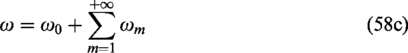
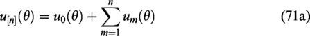
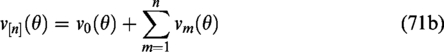
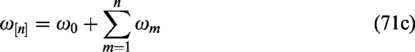
In this paper, we study the dynamical behaviors of coupled nonlinear systems with delay coupling by the multiple scales method and the homotopy analysis method. Firstly, we analyze the distribution of the eigenvalues of its linearized characteristic equations, and obtain the critical value for the occurrence of double Hopf bifurcation, which is caused by time delay and strength of coupling. Second, we obtain the normal form equations by the multiple scales method, and study the dynamical behaviors around the 3:5 weakly resonant double Hopf bifurcation point by analyzing the normal form equations. Finally, using the homotopy analysis method, we obtain analytical approximate solutions of the system with parameter values located in different regions. The periodic solution obtained by the homotopy analysis method is compared with the periodic solution obtained by the Runge–Kutta method, we found that the Runge–Kutta method does not get unstable periodic solutions, but the homotopy analysis method can be. So the homotopy analysis method is a powerful tool for studying coupled nonlinear systems with delay coupling.
Due to the practical needs of engineering applications, more and more researchers are devoted to the study of nonlinear dynamics systems, especially coupled nonlinear systems1,2 and time-delay nonlinear systems.3,4 In this paper, we study the coupled nonlinear systems with delay coupling, which is a relatively complicated issue.
In 1994, Bélair and Campbell5 studied that a first-order differential system with two time delays can present double Hopf bifurcation. Then, Xu and Chung6 declared that a time delay and feedback gain also can make double Hopf bifurcation to occur. In 2003, normal form theory was used to study non-resonance double Hopf bifurcation for a kind of differential equation with delay by Buono and Bélair.7 Szalai and Stépán8 presented a closed-form calculation for the analysis of the period-doubling bifurcation in the time-periodic delay-differential equation model of interrupted machining processes such as milling where the nonlinearity is essentially nonsymmetric. He et al.9 investigated the issue of impulsive stabilization and Hopf bifurcation of a new three-dimensional chaotic system. Ma et al.10 applied geometric method to study double Hopf bifurcation for van der Pol-Duffing oscillator with parametric delay feedback control. In recent years, more and more scholars have begun to pay close attention to the complex dynamic behaviors of coupling systems with time delay. For example, Yan and Chu11 studied a delayed Lotka–Volterra predator–prey system, and got the linear stability of equilibrium point and the character of the Hopf bifurcation solutions. Barrón and Sen2 discussed the synchronization of four coupled van der Pol oscillators. Song et al.12 and Zhang et al.13 respectively studied multiple Hopf bifurcations of three coupled van der Pol oscillators with delay. Wang and Xu14 successfully applied MMS to study double Hopf bifurcation with 1:3 resonance of coupled van der Pol oscillators with delay. That means, multiple scales method (MSM) also applies to nonlinear systems with time-delay coupling. Based on the normal form method and center manifold theorem, Li et al.15 studied the double Hopf bifurcation of a kind of coupled systems with time delay, and introduced the bifurcation diagram by numerical simulation. Ge and Xu16 studied the weakly resonance double Hopf bifurcation for a class of delay differential equations with four dimensions. Wang and Chen17 applied MSM to study the weakly resonance and non-resonance double Hopf bifurcation for a kind of seven coupled van der Pol systems with time delay. Amer et al.18 study the nonlinear vibrations of a parametric excited Duffing oscillator with time-delay feedback by the MSM.
At present, the methods of studying the nonlinear system include harmonic balance method,19 homotopy analysis method (HAM),20 perturbation incremental method,21 MSM,22 and so on. In 1992, the HAM was first put forward by Liao.23 Different from other analytical approximation method, the HAM not only overcomes the limitation of traditional methods relying on small parameter perturbation but also provides us with an additional way to conveniently adjust and control the convergence region and rate of solution series. Recently, the HAM has been widely applied for coupled nonlinear systems and time-delay nonlinear systems. For instance, You and Xu24 applied HAM to study periodic solutions of delayed differential equations that describe time-delayed position feedback on the Duffing system. It is found that the current technique leads to higher accurate prediction on the local dynamics of time-delayed systems near a Hopf bifurcation than the energy analysis method. Li25 applied HAM to solve the coupled KdV equations. Kheiri and Jabbari26 combined HAM with Padé approximation method to study a kind of two-dimensional coupled Burgers' equations. Tasbozan et al.27 obtained approximate analytical solutions of fractional coupled modifed Korteweg de Vries (mKdV) equation by HAM. Jafarian et al.28 adopted HAM to solve coupled Ramani equations, and got satisfying approximate analytical solutions. Eigoli and Khodabakhsh29 studied the limit cycle of the van der Pol oscillator with delayed amplitude limiting by HAM. Bel and Reartes30 considered a special type of second-order delay differential equations. Cobiaga and Reartes31,32 applied HAM to search periodic orbits in delay differential equations. Nave et al.33 improved HAM to study the pressure driven flame in porous media. Rajeev34 discussed the mathematical model of Stefan problem with fractional order derivatives and obtained an approximate solution of the problem by the HAM. Mahendra and Patel35 discussed one-dimensional nonlinear partial differential equation for finger-imbibition phenomenon arising in a double-phase flow through a heterogeneous porous medium during secondary oil recovery process, and solved the equation with appropriate initial and boundary conditions by the HAM. Singh et al.36 applied the HAM to obtain approximate analytical solutions of the (1 + 1) dimensional nonlinear Boussinesq equation having a fractional time derivative. By taking proper values of the auxiliary and homotopy parameters, its numerical values of the state variables are computed and presented graphically for different particular cases. Fei et al.37 analyzed a sinusoidal excited piecewise linear–nonlinear oscillator, and proposed an approximate solution for the oscillator by using the HAM and matching method. The validity criteria for the application of the semi-analytic asymptotic methods are exploited,38 comparison between the solutions obtained by the two asymptotic techniques, that is, the fractional homotopy analysis transform method and the optimal HAM is performed to select the most accurate technique for the stated problem.
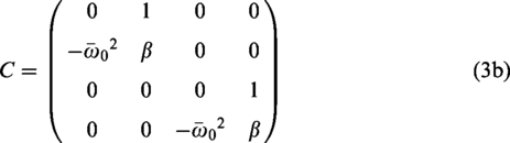
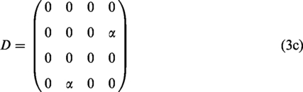
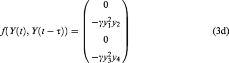
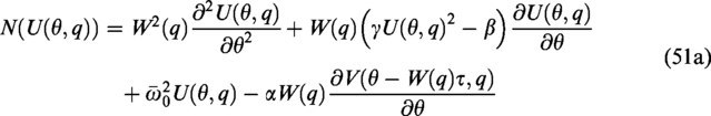
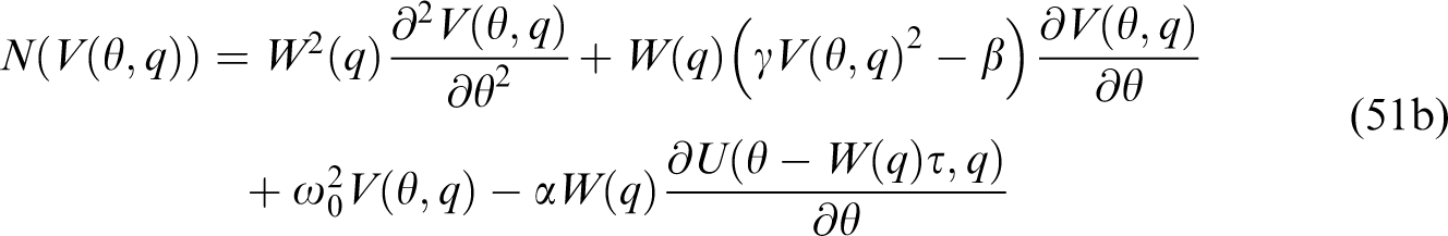
In this paper, attention is paid to a system of two coupled nonlinear systems with delay coupling, as follows:
where, is the natural frequency, is coupling intensities, is time delay, is the damping coefficient, and is nonlinear coefficient.
The constitute of the article is as follows: In The critical value for the occurrence of double Hopf bifurcation section, we analyze the distribution of the eigenvalues of its linearized characteristic equations, and get the critical value for the occurrence of double Hopf bifurcation by the Hopf bifurcation theorem, which is caused by time delay and strength of coupling. In section 3, we obtain the normal form equations by the MSM and analyzed it. At the same time, the dynamic behavior around 3:5 weak resonance double Hopf bifurcation point is studied. In application of HAM section, we obtain analytical approximate solutions of the system with parameter values located in different regions using the HAM. In numerical simulation section, via numerical simulation, the periodic solutions obtained by HAM are compared with those of Runge–Kutta method, we find that the HAM is more suitable for this system.
The critical value for the occurrence of double Hopf bifurcation
In this section, the critical value where double Hopf bifurcation occurs is obtained by studying the distribution of the eigenvalues of the associated linearizing characteristic equation.
According to the definition of double Hopf bifurcation and the bifurcation analysis of a four-neuron delayed system, the following conclusions hold.
Conclusion 1: If there occurs double Hopf bifurcation of system (1), it must meet .
Proof: Let then the system (1) can be represented as:
Let
Then the system (1) can be further represented as
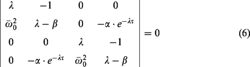
Hence, the characteristic equation of linear part of the system is as follows:
where is a unit matrix.
That means
Simplifying it, we can get
As we know, if there occurs double Hopf bifurcation of system (1), then it means that equation (7) has two and only two purely imaginary eigenvalues.
Assume that the pure imaginary numbers , are pair solutions of equation (7), and substitute them into equation (7). Based on , separate real and imaginary parts, then we can obtain
According to we can get
Let and substitute it into equation (9), we can gain
Considering we can come to a conclusion: When , equation (10) has two and only two nonnegative roots, as follows
Accordingly, equation (7) has two and only two purely imaginary eigenvalues
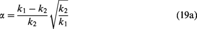
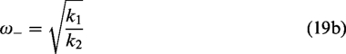
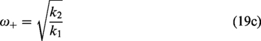
where, , , .
Hence, a conclusion can be drawn that if there occurs double Hopf bifurcation of system (1), it must meet . □
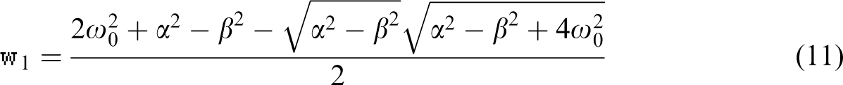
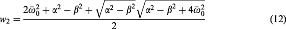
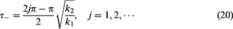
Further, let , where and are relatively prime positive integers, and . Accordingly, . Substituting them into equations (11) and (12), we can gain
It is clear that when and are selected, based on the above formula, can be expressed as a function of , such as .
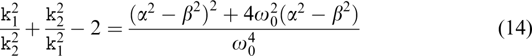
Substituting into equations (12) and (13), we can accordingly get and . Substituting them into equation (8), we can gain
Based on the Hopf bifurcation theorem, a sufficient condition of double Hopf bifurcation of system (equation (1)) is , that is, when equations (15) and (16) are equal. According to this conclusion, we can get the suitable numerical value of , and then determine whether the system has the double Hopf bifurcation with resonance.
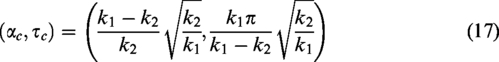
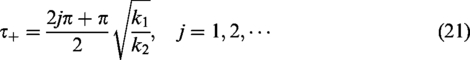
Conclusion 2: When , , there exists a double Hopf bifurcation with resonance of system (1), and the bifurcation point is
where , , .
Proof: Simplicity, Let
then
And further, we can obtain
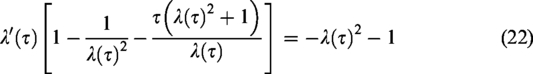
Differentiating with respect to in equation (7), these can be obtained
and
Then
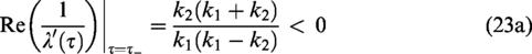
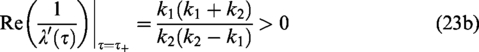
Further, when , it yields
accordingly
Therefore, when , , there exists a double Hopf bifurcation with resonance of system (1), and the bifurcation point is
where , , . □
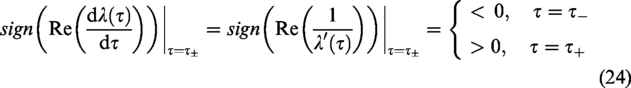
Based on Conclusion 2, we can obtain some double Hopf bifurcation points of system (1), as shown in Figure 1.
The double Hopf bifurcation points for different .
MSM and normal form equations
In this section, we obtain the normal form equations by the MSM and analyzed it. At the same time, the dynamic behaviors around 3:5 weak resonance double Hopf bifurcation point is studied.
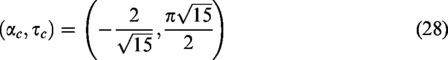
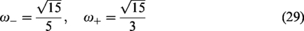
Based on conclusion 2, it is known that when , , there exists a double Hopf bifurcation with 3:5 weak resonance of system (1), and the bifurcation point is
with
For the convenience of calculation, set .
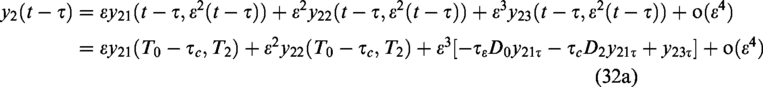
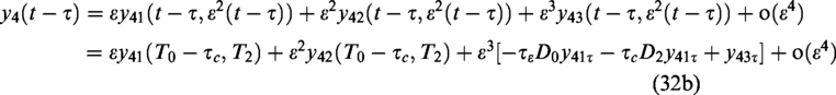
According to MSM, the solution of equation (2) can be expressed as below:
where
While the bifurcation parameters are ordered as
The delay term in equation (2) can be further Taylor expanded as
where ,
By substituting equations (30) –(32) into equation (2), Taylor expanding the new formula as well and equating separately coefficients of the same powers of , the following perturbative equations are obtained:
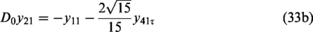
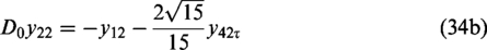
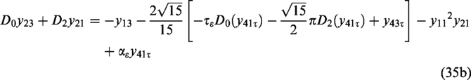
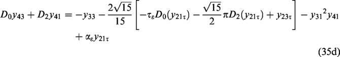
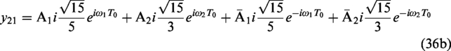
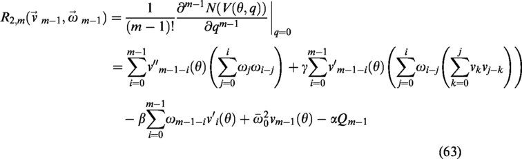
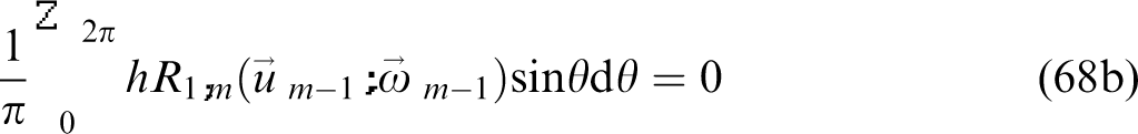
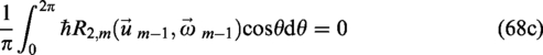
Substituting equations (36) into equations (34) and (35), and eliminating the secular terms , we can obtain the equations including and :
where the complex coefficients are expressed as follow:
For expressing the complex amplitude equations in real form, a mixed form representation of the complex amplitudes is introduced:
Substituting equation (39) into equation (37) and separating the real and imaginary parts, the normal form equations are drawn:
Let , then we can obtain all possible equilibrium points of equation (40):
where
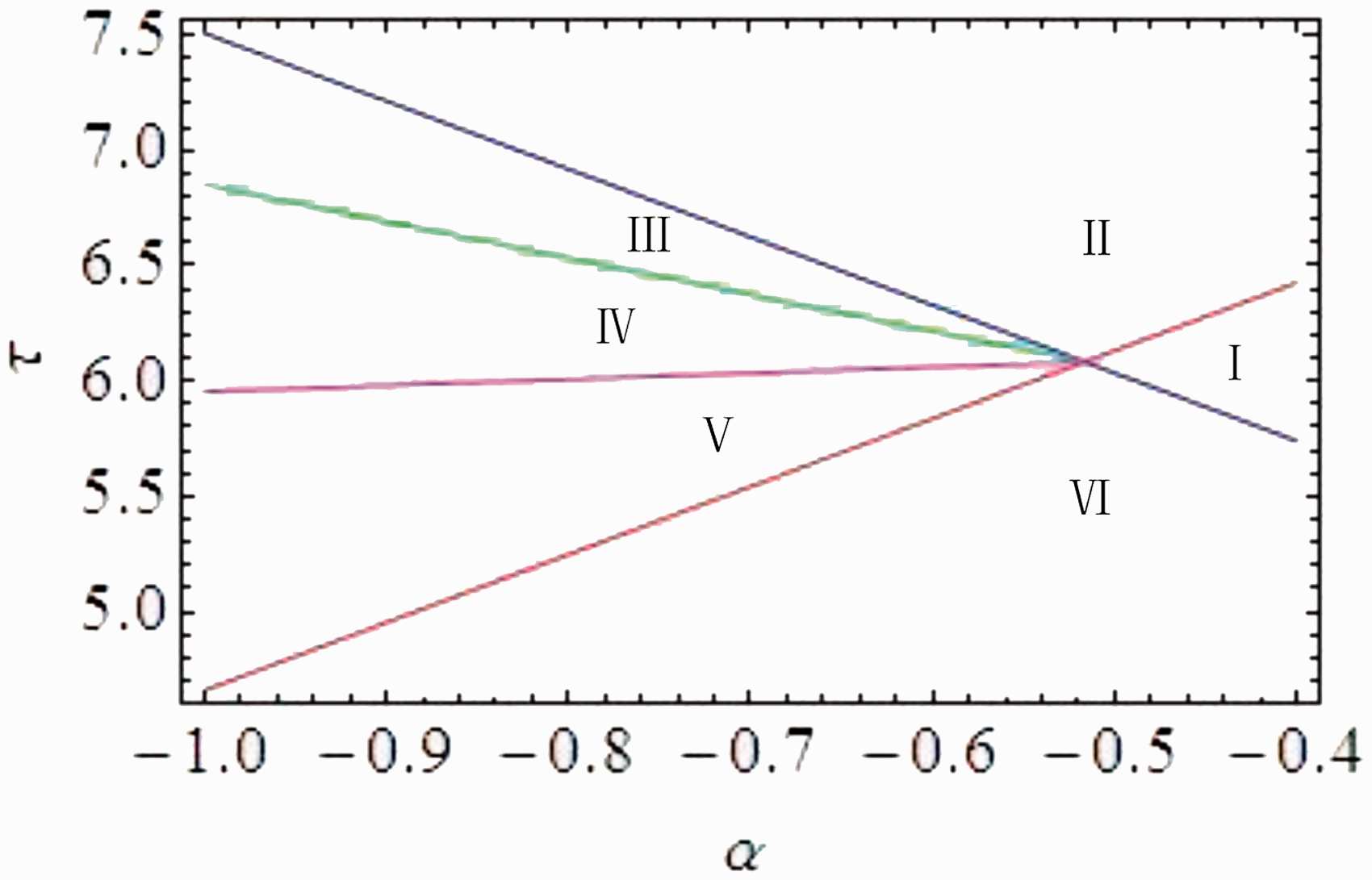
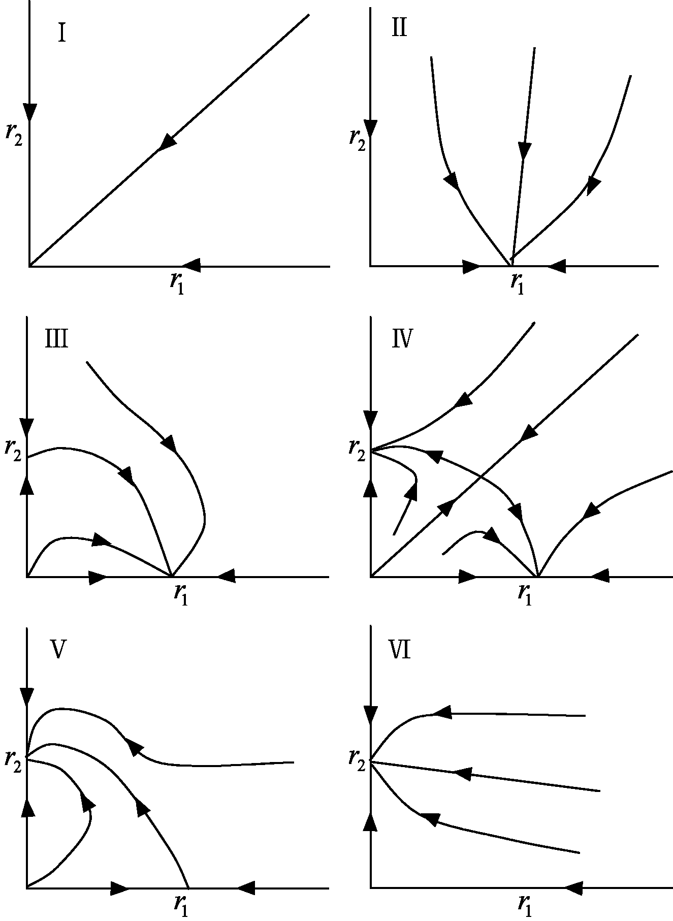
The existence of the above possible equilibrium points is dependent on and . And according to the stability analysis of existing equilibrium points, the parameters plane around the 3:5 weakly resonant double Hopf bifurcation point can be divided into six distinct dynamical regions as shown in Figures 2 and 3. The solutions in the same region have the same topological structure.
The dynamical behaviors around the 3:5 weakly resonant double Hopf bifurcation point .
Classification of intrinsic dynamic behavior around the 3:5 weakly resonant double Hopf bifurcation point .
In region I, there is only a trivial equilibrium point , which is stable. That means the vibration of system (1) is restricted by parameters and , so region I is usually called as an amplitude death region.
With changing into region II, the trivial equilibrium point loses its stability and a stable equilibrium point appears. Correspondingly, there is a stable periodic solution with a frequency close to .
When enters into region III, the unstable equilibrium point and the stable equilibrium point still exist, and an unstable equilibrium point appears. Correspondingly, there exists a stable periodic solution with a frequency close to and an unstable periodic solution.
In region IV, an unstable nontrivial equilibrium point appears together with two stable equilibrium points and . Correspondingly, system (1) admits two coexisting periodic oscillations and an unstable quasiperiodic motion.
With changing into region V, the equilibrium point disappears and there exist three equilibrium points, , and . In contrast with the situation in region III, the equilibrium point is unstable and is stable. Correspondingly, there exists a stable periodic solution with a frequency close to and an unstable periodic solution.
When enters into region VI, the equilibrium point disappears and there exists an unstable equilibrium point and a stable equilibrium point . Correspondingly, there is a stable periodic solution with a frequency close to .
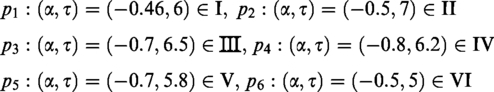
To demonstrate the above theoretical results, we choose six groups of parameter values for system (1) with , , and the results are given in Figure 4. It is obvious that numerical simulations are well consistent with the theoretical results.
The phase portraits when is located in each region.
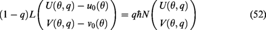
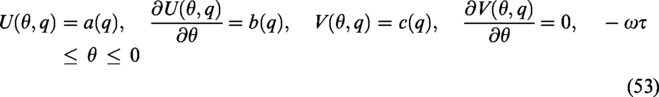
Application of HAM
Assuming system (1) satisfies the initial condition:
and the frequency of initial value solution is .
Let , then system (1) can be expressed as
with the initial condition
Suppose that the solutions of equations (45) and (46) can be expressed by the set of base functions
While for , equations (52) and (53) are equivalent to the original equations, and admit the solution
Hence, as changes from 0 to 1, and , respectively vary from the initial guess and to the unknown and . Likewise, varies from the initial guess frequency to the physical frequency .
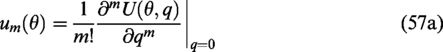
According to Taylor series expansion, we obtain
where
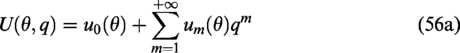
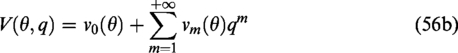
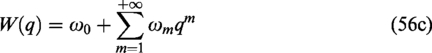
Note that the zero-order deformation equations have auxiliary parameters. Assuming is so properly chosen that power series equation (56) converge at , the series solutions of equation (56) can be expressed as
For the sake of simplicity, we define the vectors
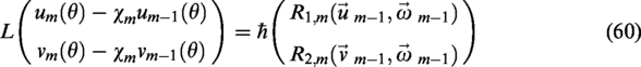
By differentiating the zeroth-order deformation equation (52) times with respect to , then dividing the equation by and setting , we arrive at the mth-order deformation equation
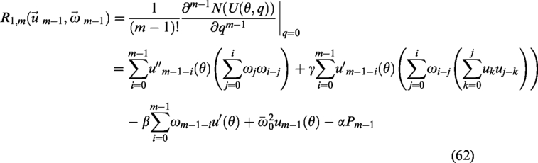
where
and the initial conditions
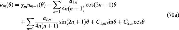
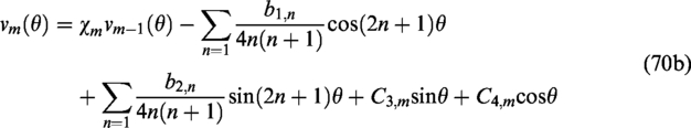
According to the rule of solution expression, and should not contain the so-called secular terms of and . Correspondingly, and should not contain the terms of and . Setting their coefficients to zeroes, we obtains
Based on equation (68), and can be obtained, for each
According to equation (68), , , , and can be expressed with respect to , , and . So, as , , and are obtained, , , , and are obtained successively, and then and are obtained.
Therefore, through the iteration step by step, the nth-order homotopy analytical approximation can be obtained, as expressed in terms of the summation series
Numerical simulation
According to the MSM and normal form equations section, parameters plane around the 3:5 weakly resonant double Hopf bifurcation point can be divided into six distinct dynamical regions, and when is located in different regions, the system (1) presents different dynamic behaviors. Now, HAM is used to obtain analytical approximate solutions of system (1) with located in each region. Since region I is an amplitude death region, it is not necessary to use HAM to approximate its exact solution. Consider that when is located in region II or VI, system (1), respectively has a stable periodic solution, but the frequency is different, so we put these two regions together to study. So is for regions III and V. For region IV, system (1) admits two coexisting periodic oscillations and an unstable quasiperiodic motion. Because the base functions of HAM in this paper are periodic functions, we just can obtain the two stable periodic analytical approximate solutions. As for the quasiperiodic analytical approximate solution, it will be the follow-up research.
The periodic solution by HAM with (α,τ) located in regions II or VI
We use the Mathematica software to the study of the subject when is located in regions IIand VI. For the region II, letting
We can get the initial value from equation (68) as follows
It means that system (1) has one periodic solution, as is in accord with the theoretical analysis in MSM and normal form equations section.
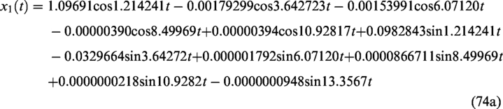
Let , the fifth-order approximation can be obtained:
The phase portrait curves of the fifth-order HAM approximation are shown in Figure 5, compared with that of fourth-order Runge–Kutta method. We found that the approximate solution agrees with the numerical solution.
Comparison of the phase portrait curves of the fifth-order HAM approximation with that of fourth-order Runge–Kutta method for , , , , .
When is located in region VI, let
According to equation (68) when , a set of initial guess is obtained
It means that system (1) has one periodic solution, as is in accord with the theoretical analysis in MSM and normal form equations section.
Let , the fifth-order approximation can be obtained:
The phase portrait curves of the fifth-order HAM approximation are shown in Figure 6, compared with that of fourth-order Runge–Kutta method. By observing Figure 6, it is clear that the fifth-order HAM approximation of is much matched to that of fourth-order Runge–Kutta method, and the same conclusion is for .
Comparison of the phase portrait curves of the fifth-order HAM approximation with that of fourth-order Runge–Kutta method for , , , , .
The periodic solution by HAM with (α,τ) located in regions III or V
We use the Mathematica software to the study of the system when is located in regions III and V. For the region III, letting
According to equation (68) when , two sets of initial guess are obtained
It means that system (1) has two periodic solutions, as is in accord with the theoretical analysis in MSM and normal form equations section.
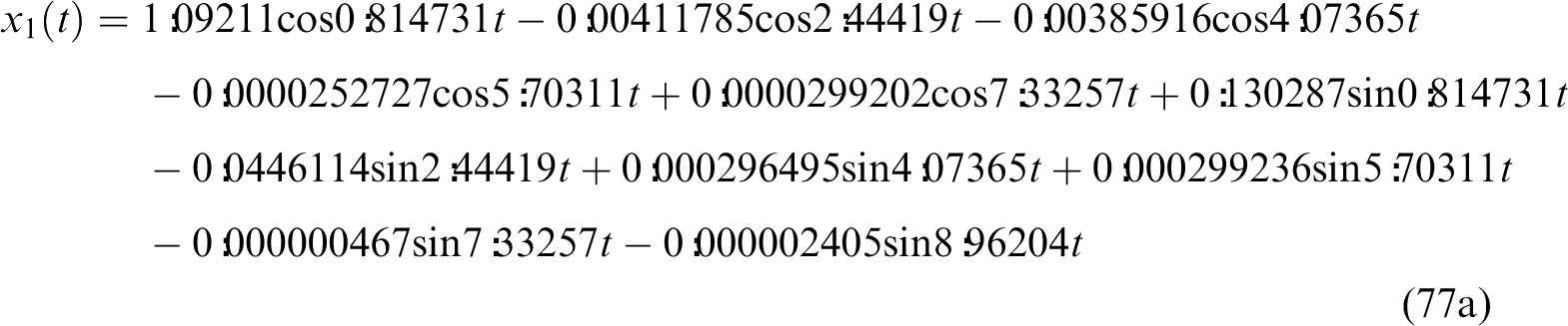
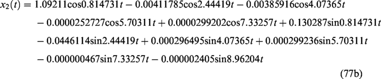
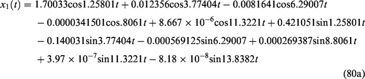
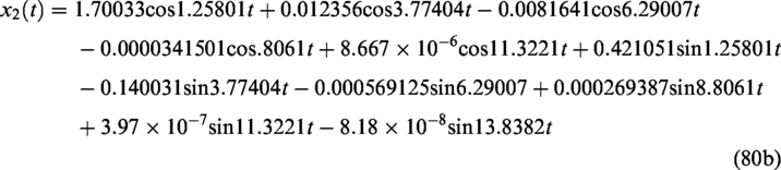
Select equation (79a) as the initial guess, and let , then the fifth-order approximation can be obtained:
Select equation (79b) as the initial guess, and let , then the fifth-order approximation can be obtained:
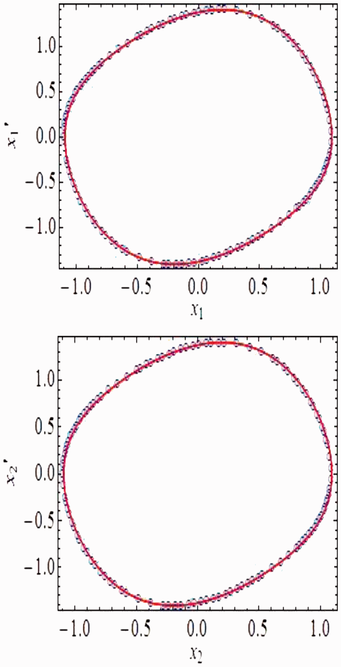
The phase portrait curves of the fifth-order HAM approximation are shown in Figure 7, compared with that of fourth-order Runge–Kutta method. Figure 7 shows that the Runge–Kutta method cannot get the unstable periodic solution, the HAM can get a stable periodic solution, but also can be unstable periodic solution. As discussed in Ebenezer et al.39 the multistep HAM allows us with great freedom to choose the convergence–control parameter ħ. Although it is plausible to optimize the HAM in other ways, the use of the convergence–control parameter ħ is the most accessible way to achieve faster convergent homotopy-series solutions. The present manuscript proposes the use of the convergence–control parameter ħ to refine the accuracy of solution series.
Comparison of the phase portrait curves of the fifth-order HAM approximation with that of fourth-order Runge–Kutta method for , , , , .
Similarly, let’s consider the condition that is located in region V. Set
According to equation (68) when , two sets of initial guess are obtained
It means that system (1) has two periodic solutions, as is in accord with the theoretical analysis in MSM and normal form equations section.
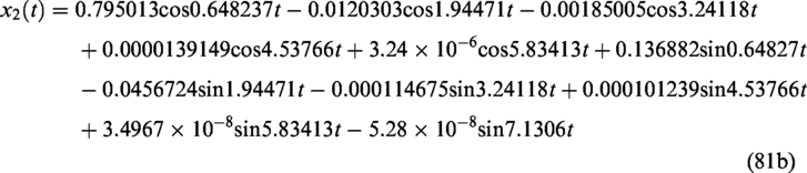
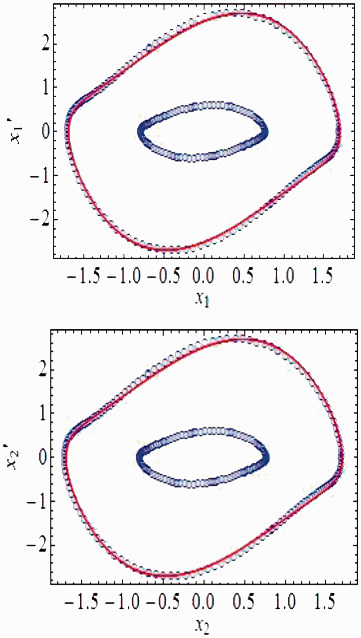
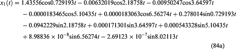
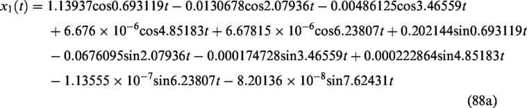
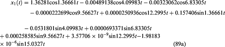
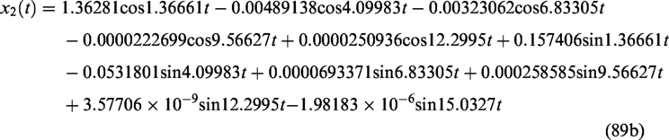
Select equation (83a) as the initial guess, and let , then the fifth-order approximation can be obtained:
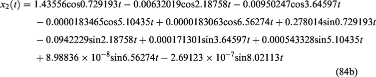
Select equation (83b) as the initial guess, and let , then the fifth-order approximation can be obtained:
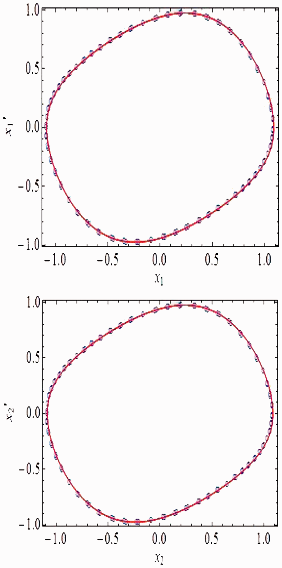
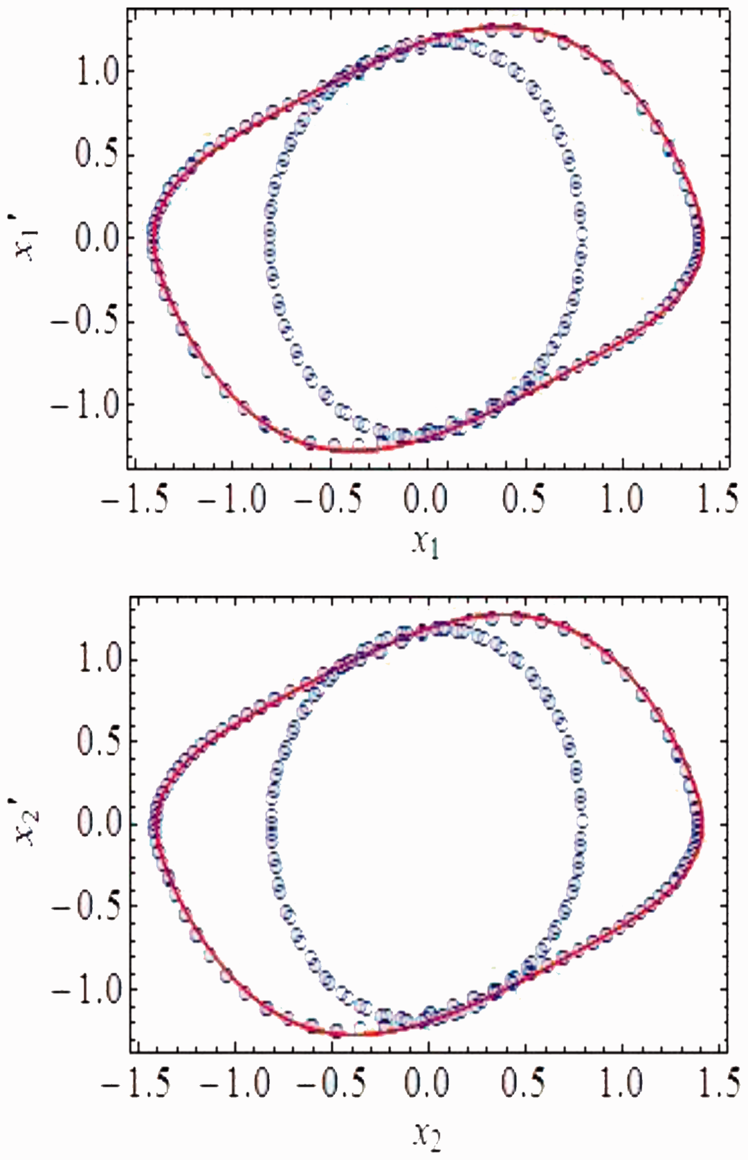
The phase portrait curves of the fifth-order HAM approximation are shown in Figure 8, compared with that of fourth-order Runge–Kutta method. It is noteworthy that traditional numerical methods such as fourth-order Runge–Kutta method cannot describe the phase portrait curve, but HAM can.
Comparison of the phase portrait curves of the fifth-order HAM approximation with that of fourth-order Runge–Kutta method for , , , , .
The periodic solution by HAM with (α,τ) located in region IV
We use the Mathematica software to the study of the subject when is located in region IV, letting
We can get two sets of the initial value from equation (60), as follows
It means that system (1) has two periodic solutions, as is in accord with the theoretical analysis in MSM and normal form equations section.
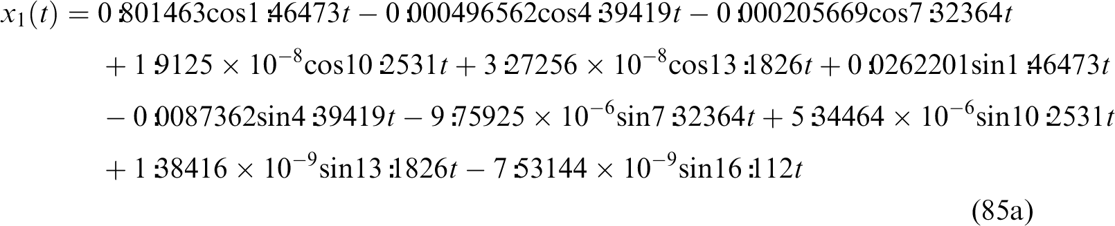
Choose equation (87a) as the initial guess, and let , then the fifth-order approximation can be obtained:
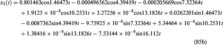
Choose equation (87b) as the initial guess, and let , then the fifth-order approximation can be obtained:
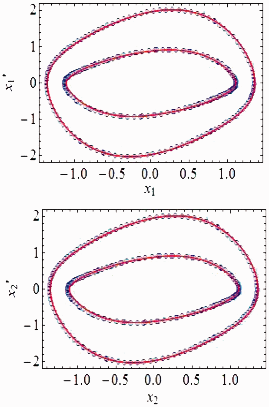
The phase portrait curves of the fifth-order HAM approximation are shown in Figure 9, compared with that of fourth-order Runge–Kutta method. We found that the approximate solution agrees with the numerical solution.
Comparison of the phase portrait curves of the fifth-order HAM approximation with that of fourth-order Runge–Kutta method for , , , , .
We obtain the periodic solution by HAM with (α,τ) located in regions II, III, IV, V, and VI. Figures 5 to 9 show that the HAM can obtain stable periodic solutions and unstable periodic solutions, but the Runge–Kutta method does not get unstable periodic solutions, so the HAM is suitable for coupled nonlinear systems with delay coupling.
Conclusions
Recently, more and more researchers are devoted to the study of nonlinear dynamical systems, especially time-delay nonlinear systems40 and coupled nonlinear systems.41,42 In this paper, we study the double Hopf bifurcation of coupled nonlinear systems with delayed coupling. Firstly, we obtain the critical value where double Hopf bifurcation occurs. Secondly, we get the normal form equations of 3:5 weakly resonant double Hopf bifurcation by the MSM. By analyzing the bifurcation equations, the dynamical behaviors of the original system are studied. It is shown that the system with has a unique zero solution when is located in region I; it has a stable periodic solution when is located in region II or VI; it has a stable periodic solution and an unstable periodic solution when is located in region III or V; it has two stable periodic solutions and an unstable quasiperiodic solution when is located in region IV. Finally, we apply the HAM to study the periodic solutions of region II to VI, and compare them with Runge–Kutta method. The results show that the HAM can obtain stable periodic solutions and unstable periodic solutions, but the Runge–Kutta method does not get unstable periodic solutions. Hence, the HAM is suitable for the system, and is a more powerful tool for the research coupled nonlinear systems with delay coupling. Due to the limit of length and energy, this article does not get the quasiperiodic analytical approximate solution in region IV, and it will be the follow-up research. The method used in this paper is only suitable for weakly resonant double Hopf bifurcation. How to obtain the strong resonant double Hopf bifurcation and use the Akbari–Ganji method43 is our next research task.
Footnotes
Acknowledgments
We are grateful to the anonymous reviewers for their constructive comments and suggestions.
Authors’ contributions
All the authors contribute equally and significantly in writing this paper. All the authors read and approve the final manuscript.
Declaration of conflicting interests
The author(s) declared no potential conflicts of interest with respect to the research, authorship, and/or publication of this article.
Funding
The author(s) disclosed receipt of the following financial support for the research, authorship, and/or publication of this article: The authors gratefully acknowledge the support of the National Natural Science Foundation of China (NNSFC) through grant No.11572288.
References
1.
KevinRRichardRHowardH.Dynamics of three coupled van der Pol oscillators with application to circadian rhythms. Commun Nonlinear Sci Numeric Simulat2007;
12: 794–803.
2.
BarronMASenM.Synchronization of four coupled van der Pol oscillators. Nonlinear Dyn2009;
56: 357–367.
3.
WeiJLiY.Hopf bifurcation analysis in a delayed Nicholson blowflies equation. Nonlinear Analysis Theory Methods Appl2005;
60: 1351–1367.
4.
JiangZWeiJ.Stability and bifurcation analysis in a delayed SIR model. Chaos Solitons Fractals2008;
35: 609–619.
5.
BélairJCampbellSA.Stability and bifurcations of equilibria in a multiple-delayed differential equation.SIAM J Appl Math1994;
54: 1402–1424.
6.
XuJChungKW.Effects of time delayed position feedback on a van Pol-Duffing oscillator. Physica D2003;
180: 17–39.
7.
BuonoPLBélairJ.Restrications and unfolding of double Hopf bifurcation in functional differential equations. J Different Equat2003;
189: 234–266.
8.
SzalaiRStépánG.Period doubling bifurcation and center manifold reduction in a time-periodic and time-delayed model of machining. J Vibrat Control2010;
16: 1169–1187.
9.
HeXHeXLiC, et al.
Impulsive control and Hopf bifurcation of a three-dimensional chaotic system. J Vibrat Contr2013;
20: 1361–1368.
10.
MaSLuQSFengZS.Double Hopf bifurcation for van der Pol Duffing oscillator with parametric delay feedback control. J Mathematica Anal Appl2008;
338: 993–1007.
11.
YanXPChuYD.Stability and bifurcation analysis for a delayed Lotka-Volterra predator-prey system. J Comput Appl Math2006;
196: 198–210.
12.
SongYLXuJZhangTH.Bifurcation, amplitude death and oscillation patterns in a system of three coupled van der Pol oscillators with diffusively delayed velocity coupling. Chaos2011;
21: 023111.
13.
ZhangCRZhengBDWangLC.Multiple Hopf bifurcation of three coupled van der Pol oscillators with delay.Appl Math Comput2011;
217: 7155–7166.
14.
WangWYXuJ.Multiple scales analysis for double Hopf bifurcation with 1: 3 resonance. Nonlinear Dyn2011;
66: 39–51.
15.
LiYQJiangWHWangHB.Double Hopf bifurcation and quasi periodic attractors in delay coupled limit cycle oscillators. J Math Anal Appl2012;
387: 1114–1126.
16.
GeJHXuJ.Weak resonant double Hopf bifurcations in an inertial four neuron model with time delay. Int J Neural Syst2012;
22: 63–75.
17.
WangWYChenLJ.Weak and non-resonant double Hopf bifurcations in m coupled van der Pol oscillators with delay coupling. Appl Math Model2015;
39: 3094–3102.
18.
AmerYAEl-SayedATKotbAA.Nonlinear vibration and of the Duffing oscillator to parametric excitation with time delay feedback. Nonlinear Dyn2016;
85: 2497–2505.
19.
LiXYZhangHBHeLJ.The principal parametric resonance of coupled van der pol oscillators under feedback control. Shock Vibrat2012;
19: 365–377.
20.
LiaoSJChwangAT.Application of homotopy analysis method in nonlinear oscillation. J Appl Mech1998;
65: 914–922.
21.
XuJChungKWChanCL.An efficient method for studying weak resonant double Hopf bifurcation in nonlinear systems with delayed feedbacks. SIAM J Appl Dyn Syst2007;
6: 29–60.
22.
RajasekarSMuraliK.Resonance behaviour and jump phenomenon in a two coupled Duffing–van der Pol oscillators. Chaos Solitons Fract2004;
19: 925–934.
23.
LiaoSJ.The proposed homotopy analysis techniques for the solution of nonlinear problems. PhD dissertation, Shanghai Jiao Tong University, Shanghai, 1992.
24.
YouXXuH.Analytical approximations for the periodic motion of the Duffing system with delayed feedback. Numer Algor2011;
56: 561–576.
25.
LiX.The application of homotopy analysis method to solve the coupled KdV equations. Int J Nonlinear Sci2011;
11: 80–85.
26.
KheiriHJabbariA.Homotopy analysis and Homotopy Padé methods for two-dimensional coupled Burgers’ equations. Iran J Mathemat Sci Informat2011;
6: 23–31.
27.
TasbozanOEsenAYagmurluNM.Approximate analytical solutions of fractional coupled mKdV equation by homotopy analysis method. OJAppS2012;
2: 193–197.
28.
JafarianAGhaderiPGolmankhanehAK, et al.
Homotopy analysis method for solving coupled Ramani equations. Roman J Phys2014;
59: 112–136.
29.
EigoliAKKhodabakhshM.A homotopy analysis method for limit cycle of the van der Pol oscillator with delayed amplitude limiting. Appl Math Computat2011;
217: 9404–9411.
30.
BelAReartesW.Isochronous bifurcations in second-order delay differential equations. Electron J Different Equat2014;
2014: 1–12.
31.
CobiagaRReartesWA.New approach in the search for periodic orbits. Int J Bifurcation Chaos2013;
23: 1350186.
32.
CobiagaRReartesW.Search for periodic orbits in delay differential equations. Int J Bifurcation Chaos2014;
24: 1450084.
33.
NaveOGol'dshteinVAjadiS.Singularly perturbed homotopy analysis method applied to the pressure driven flame in porous media. Combust Flame2015;
162: 864–873.
34.
Rajeev SinghAK.Homotopy analysis method for a fractional Stefan problem. Nonlinear Sci Lett A2017;
8: 50–59.
35.
Patel MADesaiNB. Homotopy analysis method for fingero-imbibition phenomenon in heterogeneous porous medium. Nonlinear Sci Lett A2017;
8: 90–100.
36.
SinghPKPrasadGSomT.An analytical algorithm for fractional (1 + 1) dimensional nonlinear Boussinesq equation by the homotopy analysis method. Nonlinear Sci Lett A2017;
8: 276–288.
37.
ArshadSSiddiquiAMSohailA, et al.
Comparison of optimal homotopy analysis method and fractional homotopy analysis transform method for the dynamical analysis of fractional order optical solitons. Adv Mech Eng2017;
9: 168781401769294.
38.
FeiJLinBYanS, et al.
Approximate solution of a piecewise linear-nonlinear oscillator using the homotopy analysis method. J Vibrat Contr2017; 22. DOI:10.1177/1077546317729972
39.
EbenezerB, et al.
The multi-step homotopy analysis method for a modified epidemiological model for measles disease. Nonlinear Sci Lett A2017;
8: 320–332.
40.
LiuCCYueSCZhouJL.Piezoelectric optimal delayed feedback control for nonlinear vibration of beams. J Low Freq Noise, Vibrat Active Contr2016;
35: 25–28.
41.
ShokouhiSKYuanYZhuH.Optimal placement of sensors and piezoelectric friction dampers in the pipeline networks based on nonlinear dynamic analysis. J Low Freq Noise Vibrat Active Contr2017;
35: 56–82.
42.
ZhaoLLZhouCCYueSC, et al.
Hybrid modelling of driver seat-cushion coupled system for metropolitan bus. J Low Freq Noise Vibrat Active Contr2017;
36: 214–226.
43.
NimafarM, et al.
Akbari-Ganji method for vibration under external harmonic loads. Nonlinear Sci Lett A2017;
8: 416–437.